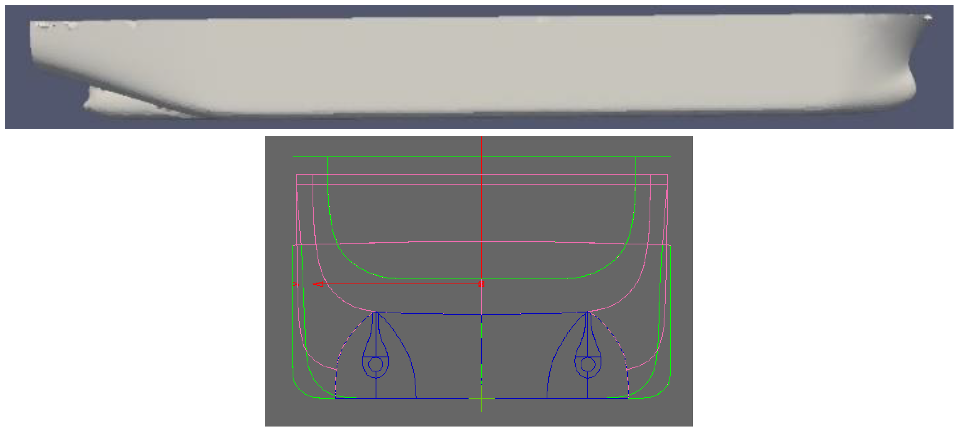
Figure 1.
Side view and lines of the 3000DWT inland bulk carrier vessel.
Figure 1.
Side view and lines of the 3000DWT inland bulk carrier vessel.
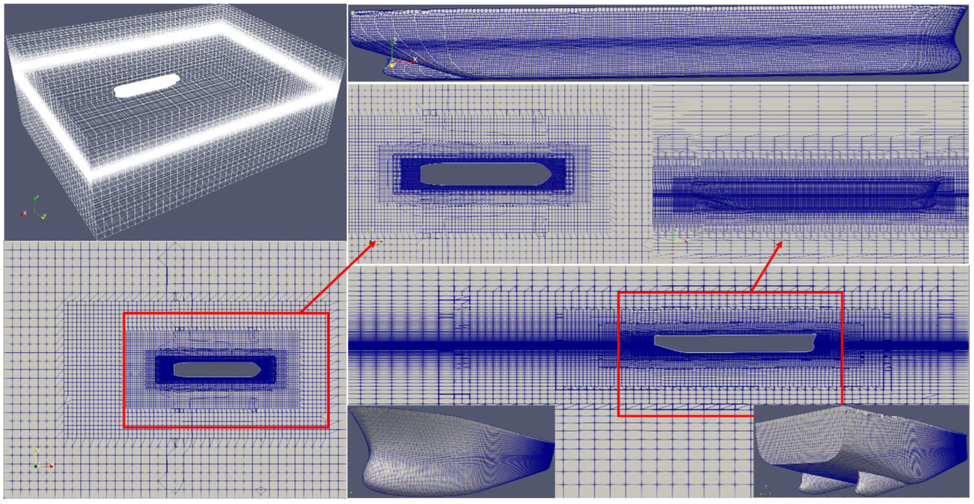
Figure 2.
General mesh assembly used in model-scale open water simulations; mesh distribution on ship hull, in the x–y plane (free surface), and the y–z plane (vertical surface). Red boxes indicate zoomed images.
Figure 2.
General mesh assembly used in model-scale open water simulations; mesh distribution on ship hull, in the x–y plane (free surface), and the y–z plane (vertical surface). Red boxes indicate zoomed images.
Figure 3.
General mesh assembly used in model-scale restricted water simulations assuming one-way (left) and two-way (right) traffic; mesh distribution on ship hull, in the x–y plane (free surface), and the y–z plane (vertical surface).
Figure 3.
General mesh assembly used in model-scale restricted water simulations assuming one-way (left) and two-way (right) traffic; mesh distribution on ship hull, in the x–y plane (free surface), and the y–z plane (vertical surface).
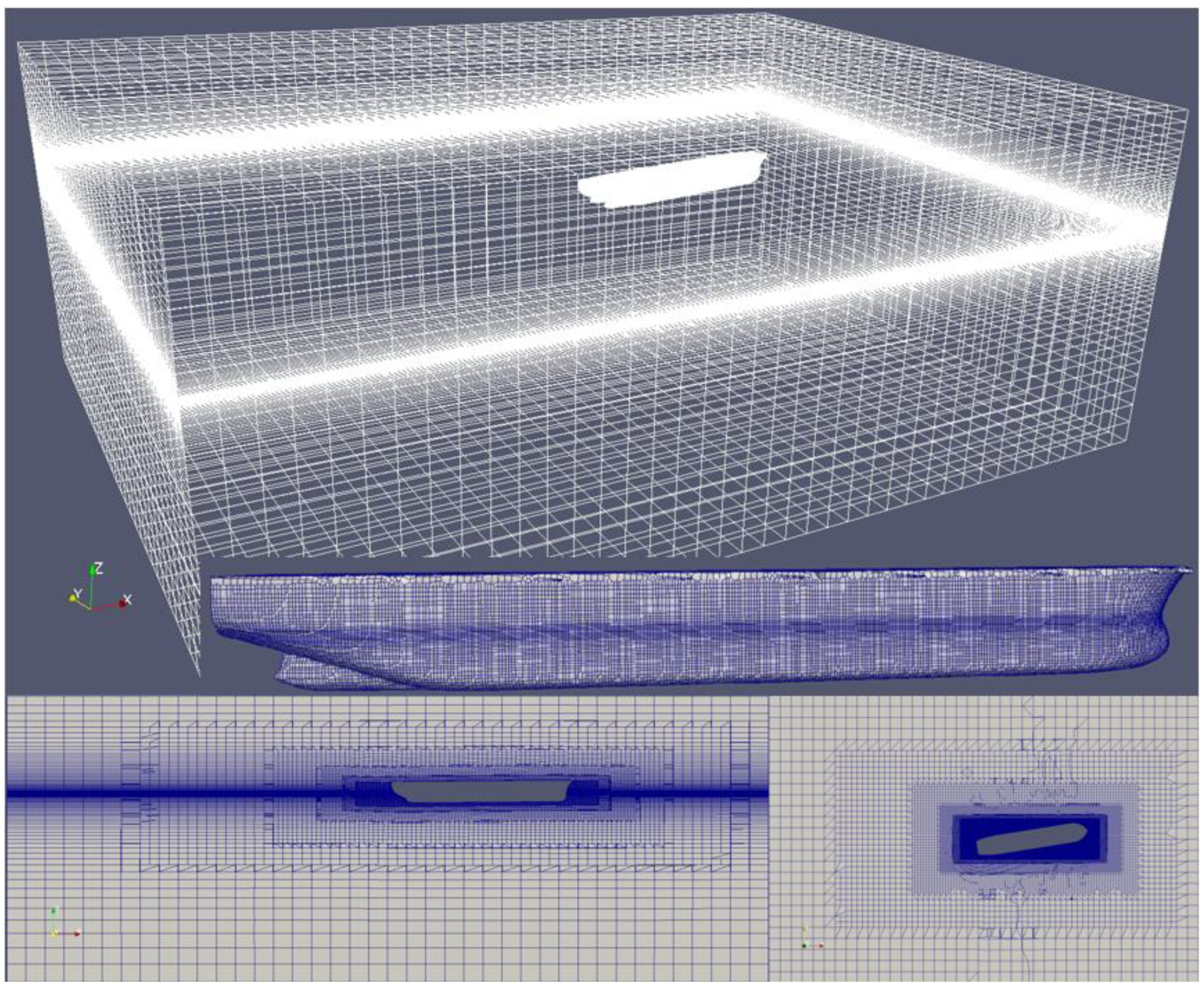
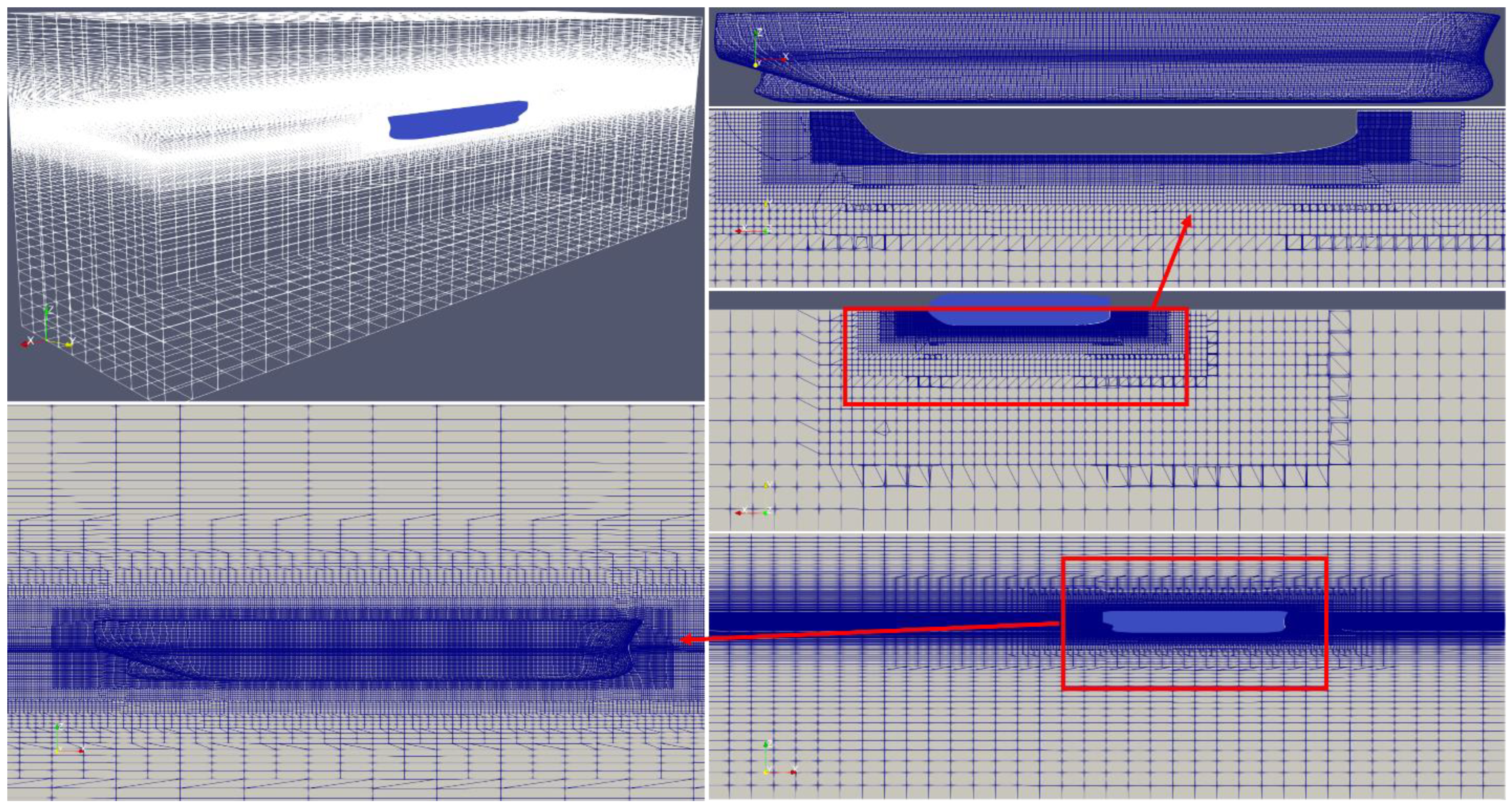
Figure 4.
General mesh assembly used in the model-scale static drift simulations, mesh distribution on hull surface, in the y–z and x–y plane.
Figure 4.
General mesh assembly used in the model-scale static drift simulations, mesh distribution on hull surface, in the y–z and x–y plane.
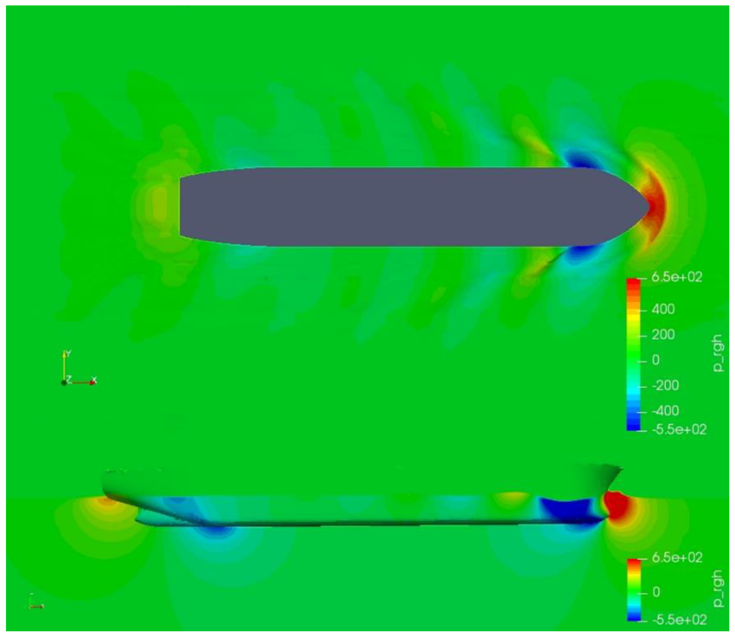
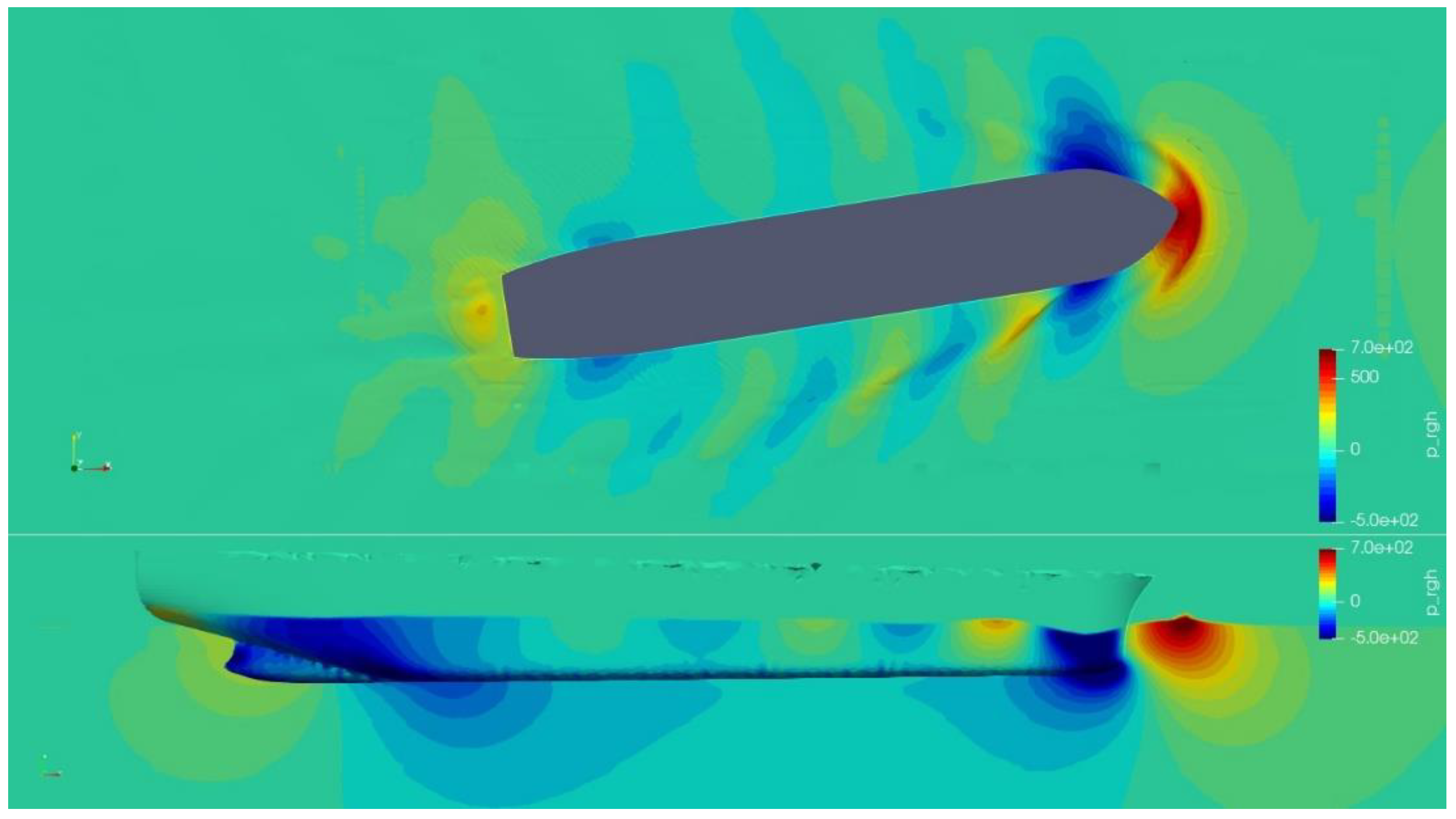
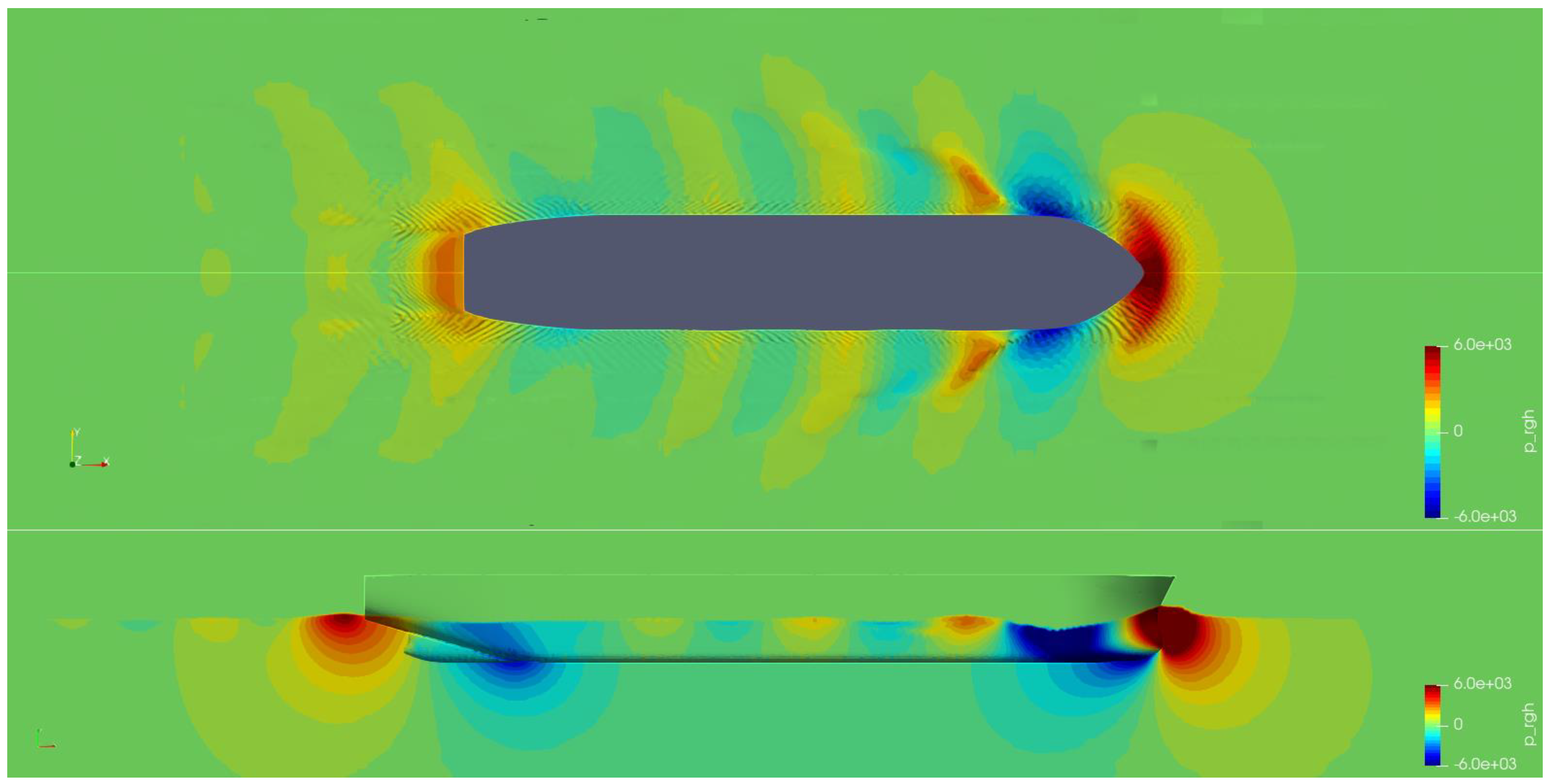
Figure 5.
Hydrodynamic pressure distribution on the free surface (above) around the hull and at the side (below) of the bulk carrier (model-scale) at Fr. 0.182.
Figure 5.
Hydrodynamic pressure distribution on the free surface (above) around the hull and at the side (below) of the bulk carrier (model-scale) at Fr. 0.182.
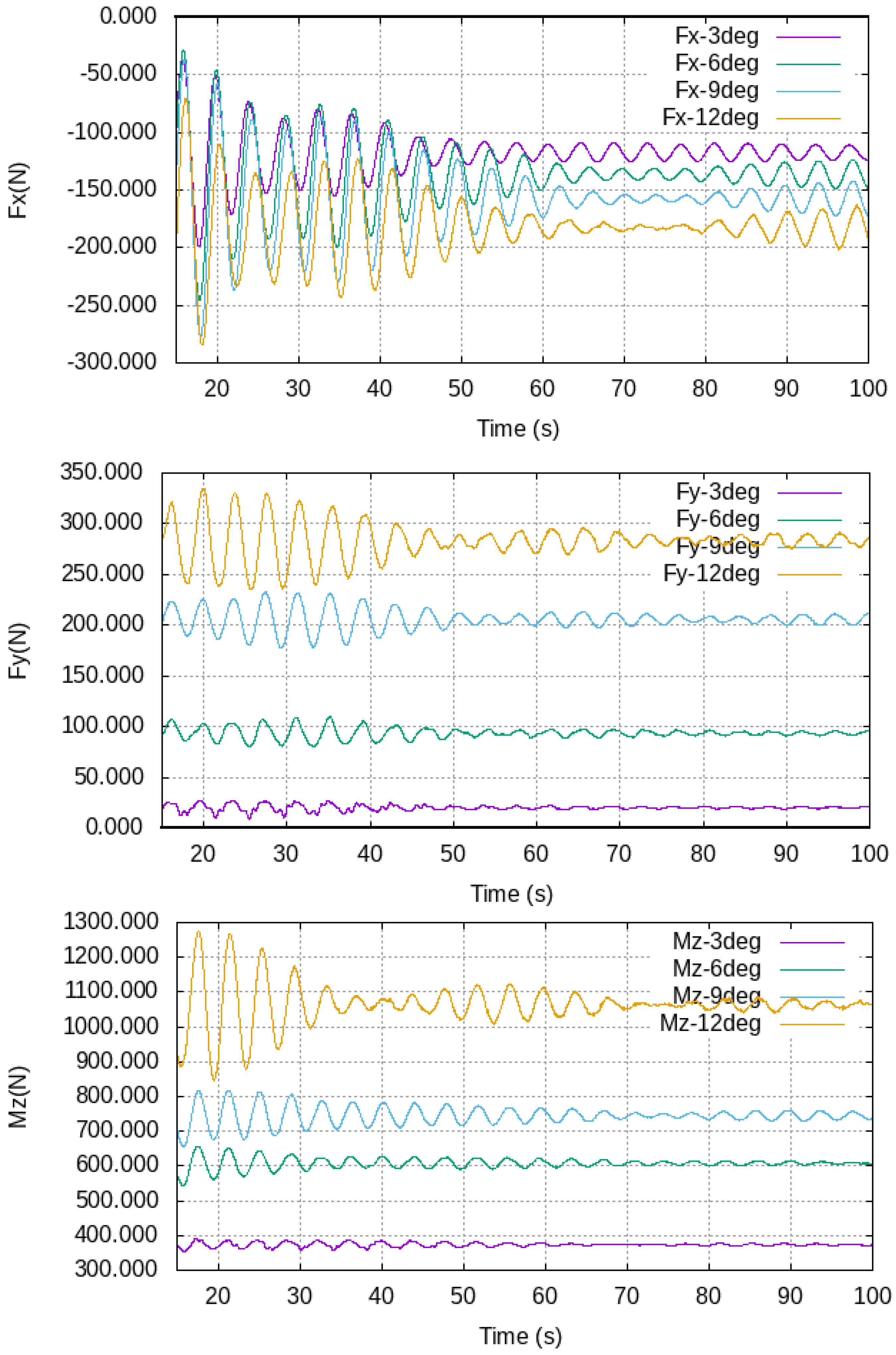
Figure 6.
Time history for surge (Fx) and sway (Fy) forces and yaw moment (Mz) for varying drift angles at Fr 0.182, respectively, from top to bottom.
Figure 6.
Time history for surge (Fx) and sway (Fy) forces and yaw moment (Mz) for varying drift angles at Fr 0.182, respectively, from top to bottom.
Figure 7.
Hydrostatic pressure distribution on the free surface around the hull and at the side of the hull (model scale) at a 9-degree drift angle and Fr. 0.182.
Figure 7.
Hydrostatic pressure distribution on the free surface around the hull and at the side of the hull (model scale) at a 9-degree drift angle and Fr. 0.182.
Figure 8.
Time history for sway (Fy) force and yaw moment (Mz) at model-scale simulations, for varying sway rates at Fr 0.182.
Figure 8.
Time history for sway (Fy) force and yaw moment (Mz) at model-scale simulations, for varying sway rates at Fr 0.182.
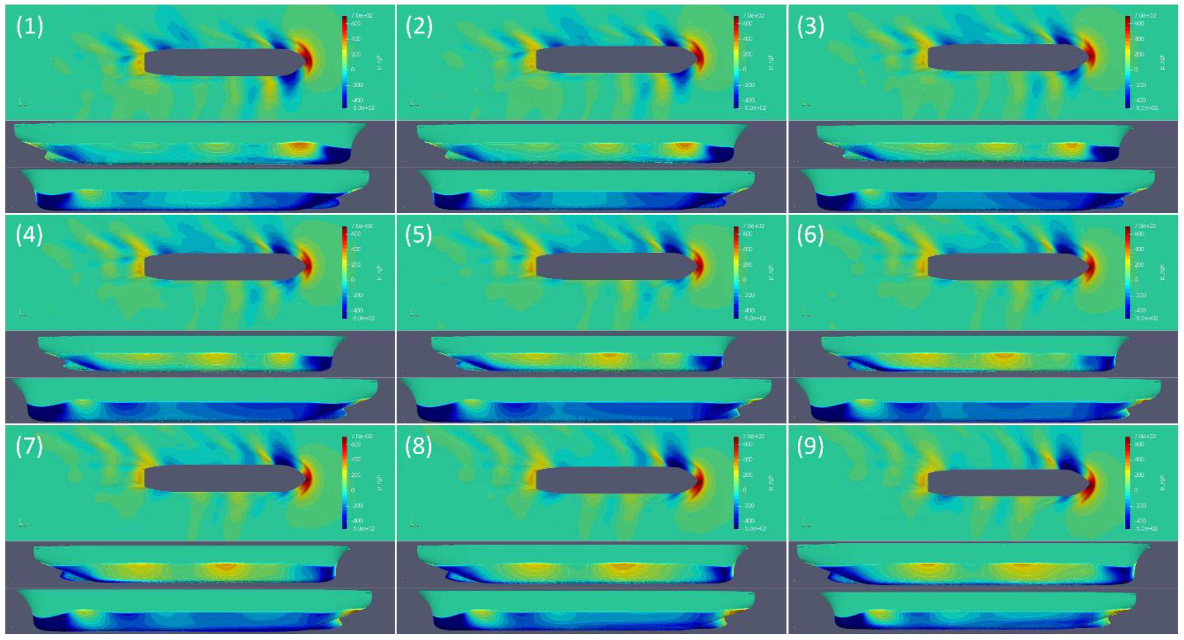
Figure 9.
Hydrostatic pressure distribution on the free surface (around the hull) and on the starboard and port side of the hull (model-scale simulations) at sway rate 0.81 and Fr. 0.182. Images 1–9 show flow field visualization with time interval of 0.2 s.
Figure 9.
Hydrostatic pressure distribution on the free surface (around the hull) and on the starboard and port side of the hull (model-scale simulations) at sway rate 0.81 and Fr. 0.182. Images 1–9 show flow field visualization with time interval of 0.2 s.
Figure 10.
Model-scale simulation time history for sway (Fy) force and yaw moment (Mz) for varying yaw rates at Fr 0.182.
Figure 10.
Model-scale simulation time history for sway (Fy) force and yaw moment (Mz) for varying yaw rates at Fr 0.182.
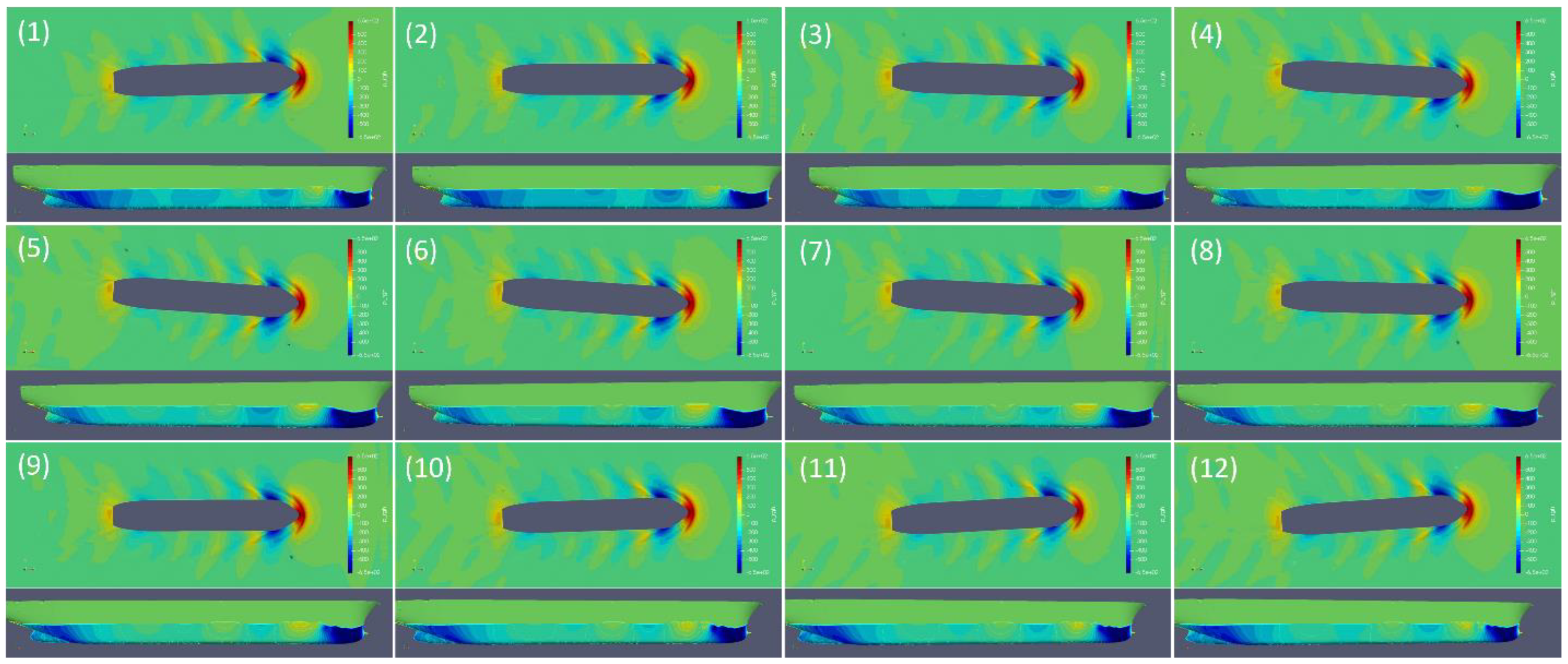
Figure 11.
Hydrostatic pressure distribution on the free surface (around the hull) and on the starboard and port side of the hull (model-scale simulations) at yaw rate 0.50 and Fr. 0.182. Images 1–12 represent flow field visualization for yaw simulation at 1 s time interval.
Figure 11.
Hydrostatic pressure distribution on the free surface (around the hull) and on the starboard and port side of the hull (model-scale simulations) at yaw rate 0.50 and Fr. 0.182. Images 1–12 represent flow field visualization for yaw simulation at 1 s time interval.
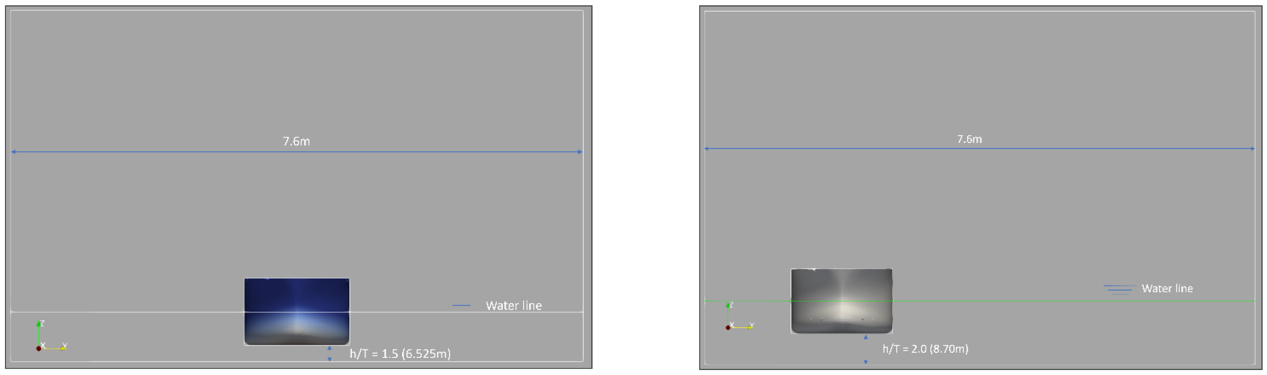
Figure 12.
Simulation domain for restricted water simulations, vessel traveling through the middle of the waterway (left) and vessel traveling close to the side of the waterway (right).
Figure 12.
Simulation domain for restricted water simulations, vessel traveling through the middle of the waterway (left) and vessel traveling close to the side of the waterway (right).
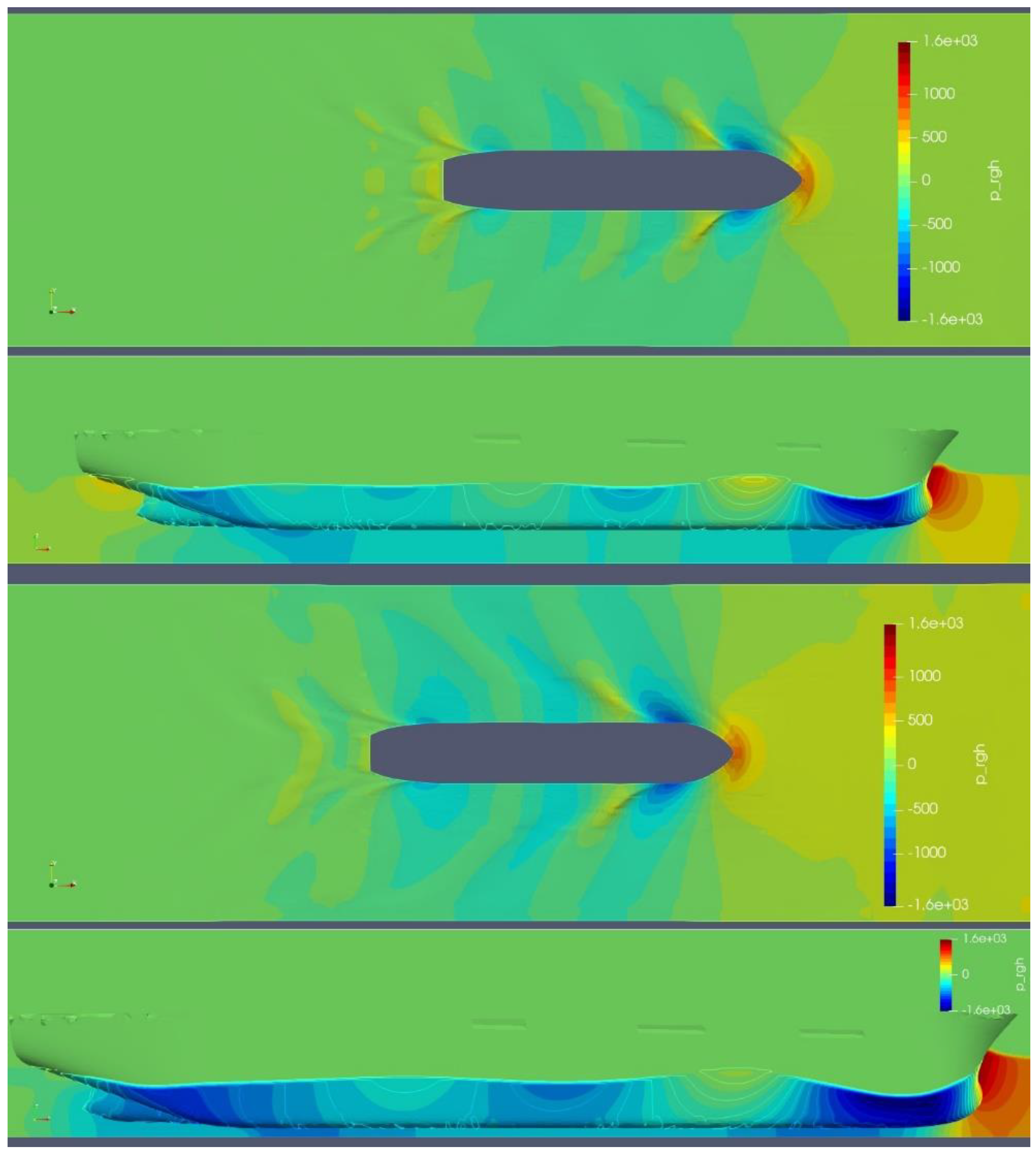
Figure 13.
Hydrodynamic pressure distribution on the water surface and on the hull in restricted simulations (model scale). The top image represents a simulation with a depth-to-draft ratio of 2.0, and the bottom image represents 1.5. Both simulations were performed at the ship design speed of 10 knots.
Figure 14.
General mesh assembly used in the full-scale open water simulations, mesh distribution on hull surface, y–z, and x–y plane.
Figure 14.
General mesh assembly used in the full-scale open water simulations, mesh distribution on hull surface, y–z, and x–y plane.
Figure 15.
Pressure distribution on the water surface and at the side of the hull at steady condition of full-scale simulation at 10 knots speed in open waters.
Figure 15.
Pressure distribution on the water surface and at the side of the hull at steady condition of full-scale simulation at 10 knots speed in open waters.
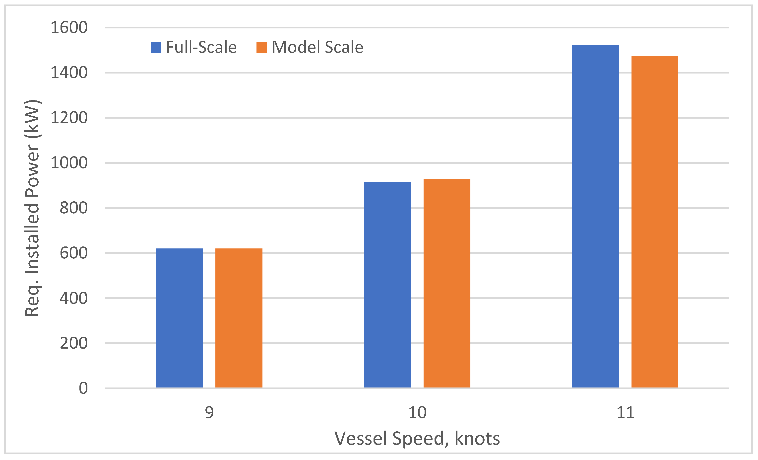
Figure 16.
Relative comparison between the propulsion power predicted by extrapolated model-scale and full-scale simulation results for three-vessel speeds.
Figure 16.
Relative comparison between the propulsion power predicted by extrapolated model-scale and full-scale simulation results for three-vessel speeds.
Table 1.
Specifications of the bulk carrier ship model.
Table 1.
Specifications of the bulk carrier ship model.
| Specification | | Bulk Carrier (Full Scale) | Bulk Carrier (Model Scale 1:10) |
|---|
| Length between perpendicular | Lpp (m) | 81.209 | 8.1209 |
| Breadth | B (m) | 14.0 | 1.4 |
| Depth | D (m) | 5.65 | 0.565 |
| Draft | T (m) | 4.35 | 0.435 |
| Wetted surface area | S (m²) | 1668.44 | 16.68 |
| Displacement volume | V (m³) | 4,335,500 | 4335.5 |
Table 2.
Specifications of mesh resolution used in different sets of simulations.
Table 2.
Specifications of mesh resolution used in different sets of simulations.
| Simulation Condition | Simulation Domain | Mesh Resolution (Million) | Minimum Cell Size
(X × Y × Z; Before Layers) | Minimum Cell Size |
|---|
| Calm water | Full hull * | 4.0 | 0.0125 × 0.025 × 0.01 | 0.0025 |
| Static Drift | Full hull * | 4.2 (average) | 0.0125 × 0.0125 × 0.01 | 0.0025 |
| Restricted water | Full hull * | 1.8 (average) | 0.0125 × 0.0125 × 0.01 | 0.0025 |
| Full-scale open water | Half hull ** | 4.0 | 0.1172 × 0.12 × 0.075 | 0.01875 |
Table 3.
Summary of the simulated cases in the study.
Table 3.
Summary of the simulated cases in the study.
| Simulation Condition | Simulation Domain | Degrees of Freedom | Froude Number | Drift Angle/Sway Rates/Yaw Rates | Depth to Draft Ratio, h/T |
|---|
| Calm water | Full hull (model scale) * | 2 (Heave and pitch-free) | 0.164, 0.182, 0.200 | 0 | 18 |
| Static Drift | Full hull (model scale) * | 2 (Heave and pitch-free) | 0.182 | 0, 3, 6, 9, 12, 15 | 18 |
| Pure Sway | Full hull (model scale) * | 0 (All motions restricted) | 0.182 | 0.1, 0.2, 0.31, 0.41, 0.61, 0.81, 0.84 | 18 |
| Pure yaw | Full hull (model scale) * | 0 (All motions restricted) | 0.182 | 0.10, 0.20, 0.30, 0.40, 0.50 | 18 |
| Restricted water | Full hull (model scale) * | 0 (All motions restricted) | 0.182 | 0 | 1.5, 2.0, 4.2 |
| Calm water | Half hull (Full scale) ** | 0 (All motions restricted) | 0.109, 0.146, 0.164, 0.182, 0.200, 0.219. | 0 | 18 |
Table 4.
Mesh settings used for the uncertainty quantification for model-scale simulations.
Table 4.
Mesh settings used for the uncertainty quantification for model-scale simulations.
| | Total Mesh (Million) | Cell Size (X × Y × Z) | Layers | Min. Cell Size | Ratio |
|---|
| Fine | 7.1 | 0.01 × 0.0099 × 0.0075 | 4 | 0.002 | 1 |
| Mid | 4.03 | 0.0125 × 0.025 × 0.01 | 4 | 0.0025 | 1.25 |
| Coarse | 1.8 | 0.0156 × 0.0156 × 0.015 | 4 | 0.00312 | 1.25 |
Table 5.
Uncertainty estimation results for the model-scale static drift simulations.
Table 5.
Uncertainty estimation results for the model-scale static drift simulations.
| Property | | Fx vis (N) | Fx tot (N) | Fy (N) | Mx (N-m) | Mz (N-m) | Sinkage (mm) | Trim (drg.) |
|---|
Output
values | Ø1 (fine) | −63.43 | −129.77 | 100.00 | 65.75 | 576.15 | −12.13 | −0.476 |
| Ø2 (mid) | −67.26 | −136.43 | 95.50 | 69.37 | 607.01 | −12.59 | −0.483 |
| Ø3 (coarse) | −59.60 | −132.96 | 94.04 | 65.94 | 601.08 | −12.49 | −0.496 |
| Convergence | ϵ21/ϵ32 | −0.50 | −1.92 | 3.08 | −1.06 | −5.20 | −4.79 | 0.54 |
Order of
accuracy | p | 3.11 | 2.92 | 5.04 | 0.26 | 7.4 | 7.02 | 2.76 |
Grid
convergence index (GCI) | GCI21fine | 0.0754 | 0.0698 | −0.0271 | 1.1521 | 0.0159 | 0.0124 | 0.0216 |
| GCI32fine | −0.1421 | −0.0346 | −0.0092 | −1.0347 | −0.0029 | −0.0025 | 0.0395 |
| Factor of safety-based approach |
Corrected
uncertainty | | 1.51% | 1.40% | −0.54% | 23.04% | 0.32% | 0.25% | 0.43% |
Corrected
uncertainty | | −2.84% | −0.69% | −0.18% | −20.69% | −0.06% | −0.05% | 0.79% |
| Correction factor-based approach |
Corrected
uncertainty | | 4.71% | 3.54% | 5.84% | 82.38% | 8.25% | 5.68% | 0.89% |
Corrected
uncertainty | | 8.88% | 1.75% | 1.98% | 73.99% | 1.50% | 1.14% | 1.62% |
Table 6.
Model-scale calm water simulation results for the ship model in open water.
Table 6.
Model-scale calm water simulation results for the ship model in open water.
| Froude | Vis F (N) | Pr F (N) | X-Force (N) | Drag Coeff. Ct | Sinkage (mm) | Trim (deg) |
|---|
| 0.164 | −51.69 | −32.60 | −84.30 | 4.72 × 10⁻³ | −8.260 | −0.52 |
| 0.182 | −64.28 | −49.43 | −113.71 | 5.16 × 10⁻³ | −11.100 | −0.49 |
| 0.200 | −77.55 | −83.06 | −160.61 | 6.02 × 10⁻³ | −14.150 | −0.44 |
Table 7.
Extrapolation of model-scale data to full scale and estimated propulsion power.
Table 7.
Extrapolation of model-scale data to full scale and estimated propulsion power.
| Froude | Vel (Knots) | Cv (Theoretical) | Ct (Scaled) | Drag Force (kN) | Drag Power (kW) | Req. Installed Power (kW) |
|---|
| 0.164 | 9.0 | 2.17 × 10⁻³ | 4.00 × 10⁻³ | 71.347 | 330.308 | 620 |
| 0.182 | 10.0 | 2.14 × 10⁻³ | 4.38 × 10⁻³ | 96.627 | 497.150 | 930 |
| 0.200 | 11.0 | 2.11 × 10⁻³ | 5.23 × 10⁻³ | 139.415 | 788.714 | 1472 |
Table 8.
Open water static drift simulation results for the model-scale 3000DWT inland bulk carrier.
Table 8.
Open water static drift simulation results for the model-scale 3000DWT inland bulk carrier.
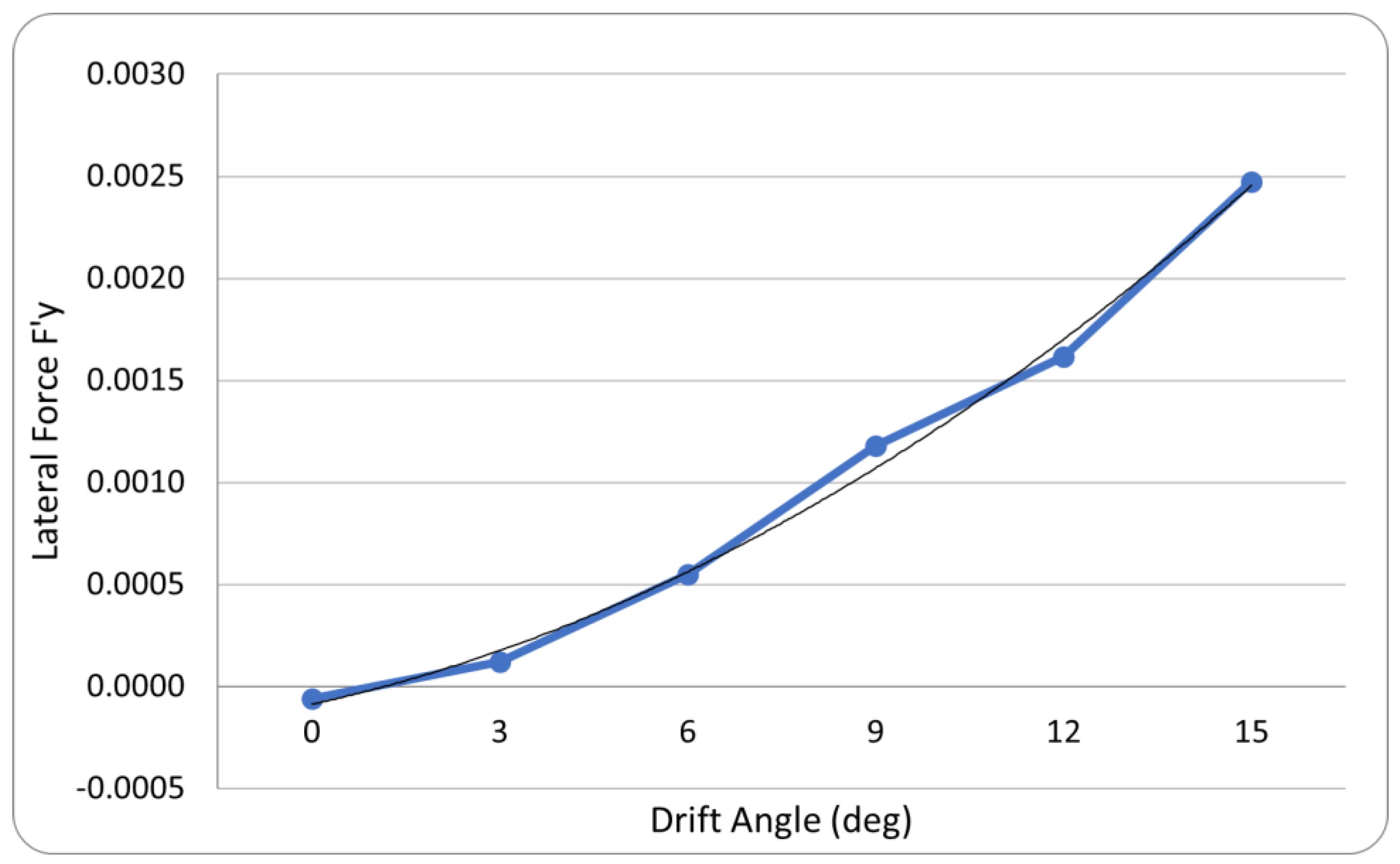
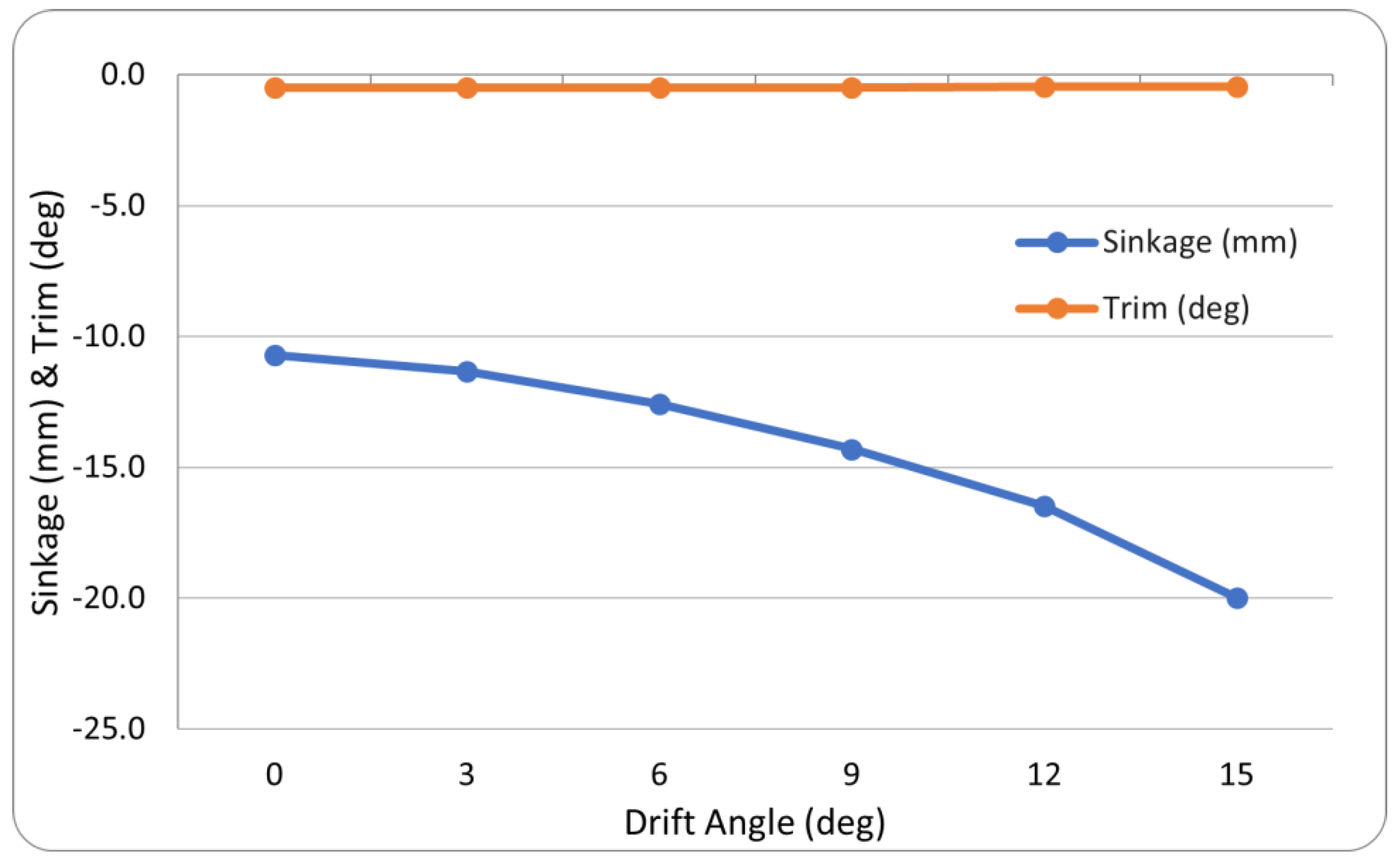
| Drift Angle | Fx-vis (N) | Fx-tot (N) | Fy (N) | F′y | Mz (N-m) | M′z | Sinkage (mm) | Trim (deg) |
|---|
| 0 | −57.370 | −111.375 | −10.55 | −6.05 × 10⁻⁵ | 34.79 | 2.46 × 10⁻⁵ | −10.720 | −0.477 |
| 3 | −64.600 | −117.328 | 21.1 | 1.21 × 10⁻⁴ | 373.54 | 2.64 × 10⁻⁴ | −11.325 | −0.480 |
| 6 | −67.260 | −136.428 | 95.5 | 5.48 × 10⁻⁴ | 607.01 | 4.29 × 10⁻⁴ | −12.585 | −0.483 |
| 9 | −67.900 | −156.560 | 205.28 | 1.18 × 10⁻³ | 744.32 | 5.26 × 10⁻⁴ | −14.300 | −0.475 |
| 12 | −62.014 | −181.291 | 281.98 | 1.62 × 10⁻³ | 1063.8 | 7.51 × 10⁻⁴ | −16.490 | −0.470 |
| 15 | −63.93 | −243.16 | 431.54 | 2.47 × 10⁻³ | 1234.08 | 8.72 × 10⁻⁴ | −20.000 | −0.470 |
Table 9.
Required power prediction for the bulk carrier during drift motions.
Table 9.
Required power prediction for the bulk carrier during drift motions.
| Drift Angle, β | Vel (Knots) | Cw (Cp) | Cv | Ct | Force Full Scale (kN) | Required Effective Power (kW) | Required Installed Power (kW) |
|---|
| 0 | 10.0 | 2.45 × 10⁻³ | 1.58 × 10⁻³ | 4.03 × 10⁻³ | 88.527 | 454.761 | 849 |
| 3 | 10.0 | 2.39 × 10⁻³ | 1.58 × 10⁻³ | 3.97 × 10⁻³ | 87.254 | 448.221 | 836 |
| 6 | 10.0 | 3.14 × 10⁻³ | 1.58 × 10⁻³ | 4.71 × 10⁻³ | 103.643 | 532.410 | 993 |
| 9 | 10.0 | 4.02 × 10⁻³ | 1.58 × 10⁻³ | 5.60 × 10⁻³ | 123.074 | 632.227 | 1180 |
| 12 | 10.0 | 5.41 × 10⁻³ | 1.58 × 10⁻³ | 6.99 × 10⁻³ | 153.595 | 789.014 | 1472 |
| 15 | 10.0 | 8.13 × 10⁻³ | 1.58 × 10⁻³ | 9.70 × 10⁻³ | 213.361 | 1096.029 | 2045 |
Table 10.
Open water pure sway simulation results for the model-scale 3000DWT inland bulk carrier.
Table 10.
Open water pure sway simulation results for the model-scale 3000DWT inland bulk carrier.
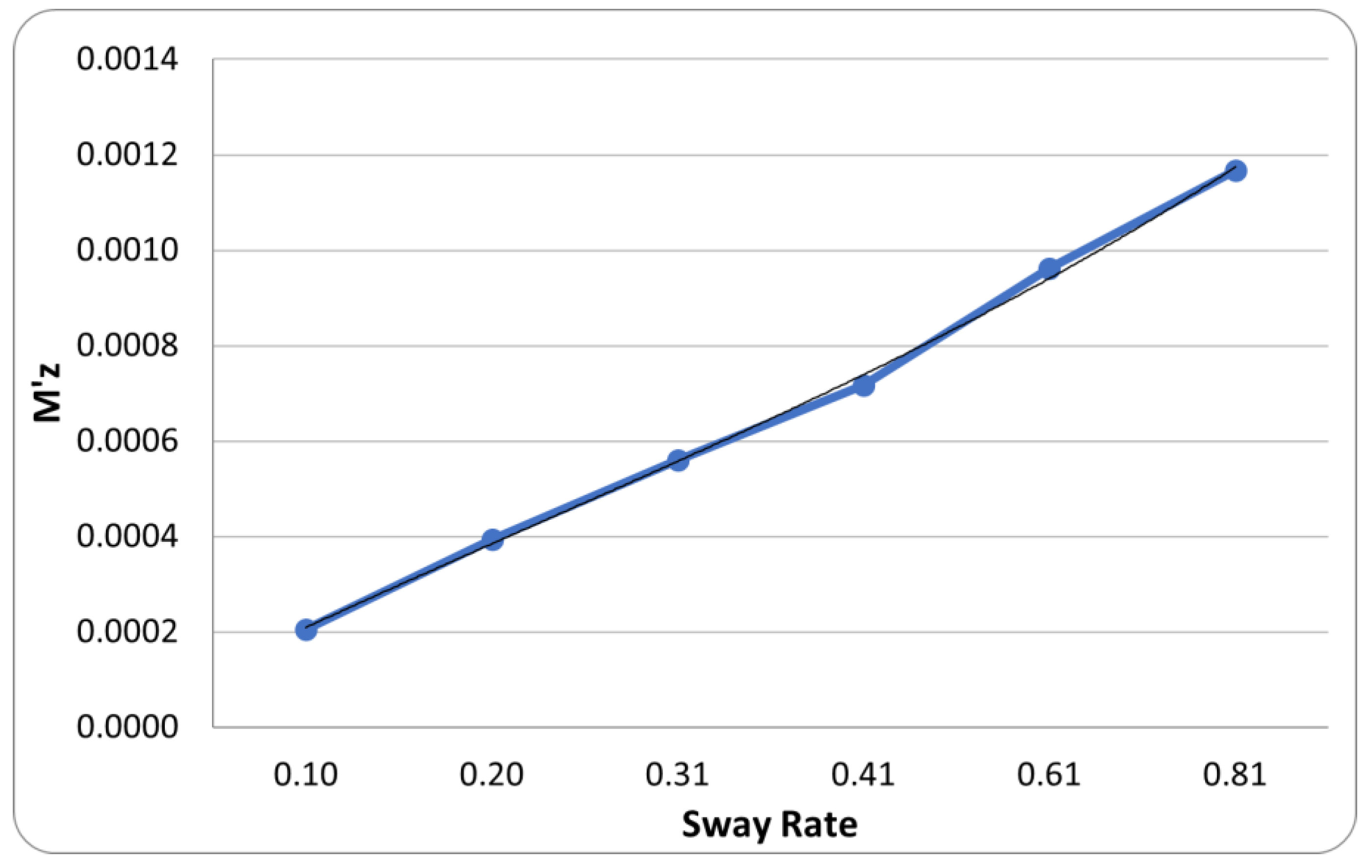
| Sway Rate, v′ | Fx-vis (N) | Fx-tot (N) | F′y | M′x | M′z |
|---|
| 0.10 | −63.487 | −113.664 | 6.27 × 10⁻⁴ | 3.44 × 10⁻³ | 2.05 × 10⁻⁴ |
| 0.20 | −64.054 | −116.074 | 1.41 × 10⁻³ | 6.88 × 10⁻³ | 3.93 × 10⁻⁴ |
| 0.31 | −64.760 | −118.625 | 2.02 × 10⁻³ | 1.03 × 10⁻² | 5.60 × 10⁻⁴ |
| 0.41 | −66.080 | −122.470 | 2.61 × 10⁻³ | 1.38 × 10⁻² | 7.16 × 10⁻⁴ |
| 0.61 | −68.460 | −129.670 | 3.84 × 10⁻³ | 2.07 × 10⁻² | 9.63 × 10⁻⁴ |
| 0.81 | −71.014 | −136.070 | 5.23 × 10⁻³ | 2.72 × 10⁻² | 1.17 × 10⁻³ |
| 0.84 | −71.88 | −137.36 | 5.43 × 10⁻³ | 2.82 × 10⁻² | 1.21 × 10⁻³ |
Table 11.
Simulation parameter settings and resistance results for pure yaw simulations of the bulk carrier.
Table 11.
Simulation parameter settings and resistance results for pure yaw simulations of the bulk carrier.
| Yaw Rate, r′ | Angle (deg) | Omega (Hz) | Displacement (m) | rdot′ | Fx-vis (N) | Fx-tot (N) |
|---|
| 0.10 | 2 | 0.0913 | 0.0990 | 0.2865 | −64.00 | −120.31 |
| 0.20 | 2 | 0.1827 | 0.0495 | 1.1459 | 64.25 | −117.53 |
| 0.30 | 2 | 0.2740 | 0.0330 | 2.5783 | −64.25 | −117.04 |
| 0.40 | 2 | 0.3654 | 0.0247 | 4.5837 | −64.40 | −119.27 |
| 0.50 | 2 | 0.4567 | 0.0198 | 7.1620 | −61.87 | −117.87 |
Table 12.
Simulation results for lateral force and yaw moment for the bulk carrier with varying yaw rates.
Table 12.
Simulation results for lateral force and yaw moment for the bulk carrier with varying yaw rates.
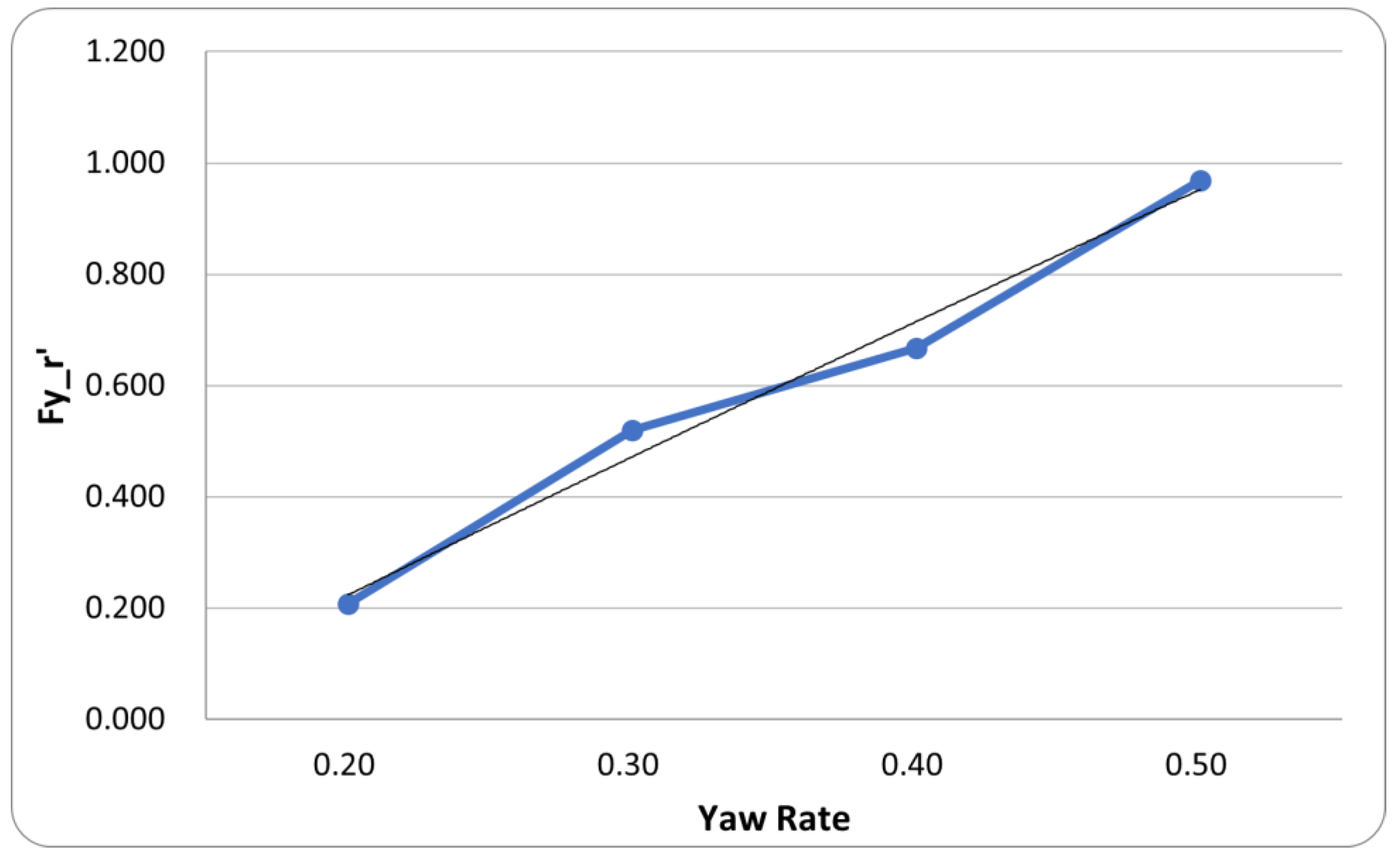
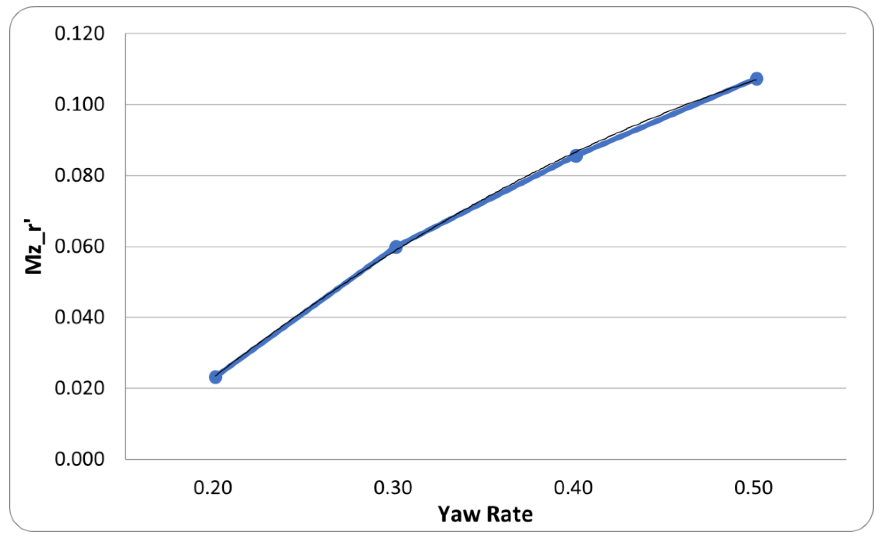
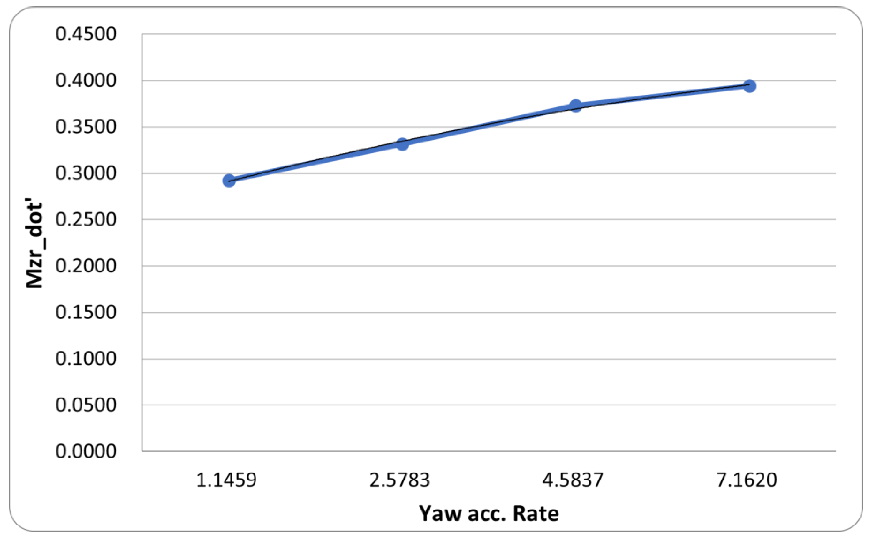
| Yaw Rate, r′ | Fy_r′ (×10−3) | Mz_r′ (×10−3) | Fyr_dot′ (×10−3) | Mzr_dot′ (×10−3) |
|---|
| 0.10 | 0.148 | 0.0155 | 0.065 | 0.2239 |
| 0.20 | 0.208 | 0.0232 | 0.172 | 0.2925 |
| 0.30 | 0.519 | 0.0600 | 0.209 | 0.3313 |
| 0.40 | 0.668 | 0.0856 | 0.232 | 0.3729 |
| 0.50 | 0.968 | 0.1073 | 0.354 | 0.3944 |
Table 13.
Manoeuvring derivatives computed for the inland bulk carrier from model-scale PMM simulations.
Table 13.
Manoeuvring derivatives computed for the inland bulk carrier from model-scale PMM simulations.
| | Derivatives | OpenFOAM Results |
|---|
| Drift | Yv | 0.00008 |
| Nv | 0.0002 |
| Sway | | 0.0012 |
| 0.0002 |
| Yaw | | 0.2561 |
| 0.0465 |
| −0.0494 |
| 0.0563 |
Table 14.
Calm water resistance simulation results for the inland bulk carrier in restricted waters.
Table 14.
Calm water resistance simulation results for the inland bulk carrier in restricted waters.
| Case | Vel (m/s) | Froude | Rn | h/T | Width (m) | Vis F (N) | Pr F (N) | X-Force (N) |
|---|
| 1 | 1.627 | 0.182 | 1.32 × 10⁷ | 2.0 | 7.60 | −74.31 | −192.74 | −267.05 |
| 2 | 1.627 | 0.182 | 1.32 × 10⁷ | 1.5 | 7.60 | −86.11 | −445.32 | −531.43 |
| 3 | 1.627 | 0.182 | 1.32 × 10⁷ | 4.2 | 7.6_side | −63.50 | −87.26 | −150.76 |
| 4 | 1.627 | 0.182 | 1.32 × 10⁷ | 2.0 | 7.6_side | −74.56 | −235.36 | −309.92 |
Table 15.
Extrapolated full-scale power requirement for the vessel while navigating through inland restricted waters.
Table 15.
Extrapolated full-scale power requirement for the vessel while navigating through inland restricted waters.
| Case | Knots | Cv (Theo) | Ct (Scaled) | Drag Force (kN) | Required Effective Power (kW) | Required Installed Power (kW) |
|---|
| 1 | 10 | 4.13 × 10⁻³ | 1.29 × 10⁻² | 192.735 | 991.627 | 1850 |
| 2 | 10 | 4.48 × 10⁻³ | 2.47× 10⁻² | 544.068 | 2799.242 | 5225 |
| 3 | 10 | 3.73 × 10⁻³ | 7.69 × 10⁻³ | 169.597 | 872.581 | 1628 |
| 4 | 10 | 4.13 × 10⁻³ | 1.48 × 10⁻² | 326.362 | 1679.140 | 3135 |
Table 16.
Mesh settings used for the uncertainty quantification for full-scale simulations (half hull).
Table 16.
Mesh settings used for the uncertainty quantification for full-scale simulations (half hull).
| | Total Mesh (Million) | Cell Size (X × Y × Z) | Layers | Min. Cell Size | Ratio |
|---|
| Fine | 8.89 | 0.0922 × 0.0919 × 0.06 | 3 | 0.015 | 1.00 |
| Mid | 4.03 | 0.1172 × 0.12 × 0.075 | 3 | 0.01875 | 1.25 |
| Coarse | 1.83 | 0.156 × 0.156 × 0.1 | 3 | 0.025 | 1.33 |
Table 17.
Uncertainty estimation results for the full-scale calm water simulations (half hull).
Table 17.
Uncertainty estimation results for the full-scale calm water simulations (half hull).
| Property | | F-Viscous | F-Pressure | F-Total |
|---|
| Output values | Ø1 (fine) | −22,960.60 | −22,924.70 | −45,885.3 |
| Ø2 (mid) | −22,726.60 | −24,952.10 | −47,678.7 |
| Ø3 (coarse) | −22,636.60 | −24,777.80 | −47,414.4 |
| Convergence | ϵ21/ϵ32 | 2.60 | −11.63 | −6.79 |
| Order of accuracy | p | 3.64 | 9.35 | 7.30 |
| Grid convergence index (GCI) | GCI21fine | −0.0080 | 0.0106 | 0.0086 |
| GCI32fine | −0.0030 | −0.0008 | −0.0012 |
| Factor of safety-based approach |
| Corrected uncertainty | | −0.16% | 0.21% | 0.17% |
| Corrected uncertainty | | −0.06% | −0.02% | −0.02% |
| Correction factor-based approach |
| Corrected uncertainty | | 0.85% | 12.08% | 5.03% |
| Corrected uncertainty | | 0.32% | 0.93% | 0.69% |
Table 18.
Open water full-scale simulation results for the inland bulk carrier.
Table 18.
Open water full-scale simulation results for the inland bulk carrier.
| Case | Vel (Knots) | Vel (m/s) | Froude | Rn | Vis F (kN) | Pr F (kN) | X-Force (kN) |
|---|
| 1 | 6 | 3.09 | 0.109 | 2.50 × 10⁸ | −12.125 | −14.313 | −26.438 |
| 2 | 8 | 4.12 | 0.146 | 3.33 × 10⁸ | −29.712 | −25.277 | −54.989 |
| 3 | 9 | 4.63 | 0.164 | 3.74 × 10⁸ | −36.083 | −35.772 | −71.855 |
| 4 | 10 | 5.14 | 0.182 | 4.16 × 10⁸ | −45.453 | −49.904 | −95.357 |
| 5 | 11 | 5.65 | 0.200 | 4.57 × 10⁸ | −53.769 | −90.540 | −144.309 |
| 6 | 12 | 6.17 | 0.219 | 4.99 × 10⁸ | −66.061 | −149.741 | −215.802 |
Table 19.
Power prediction for the inland bulk carrier from open water full-scale simulations.
Table 19.
Power prediction for the inland bulk carrier from open water full-scale simulations.
| Vel (Knots) | Ct | Cp | Cv | Cv (Theor.) | Drag Power (kW) | Req. Installed Power (kW) |
|---|
| 6 | 3.32 × 10⁻³ | 1.80 × 10⁻³ | 1.52 × 10⁻³ | 2.29 × 10⁻³ | 81.695 | 152 |
| 8 | 3.89 × 10⁻³ | 1.79 × 10⁻³ | 2.10 × 10⁻³ | 2.20 × 10⁻³ | 226.555 | 423 |
| 9 | 4.02 × 10⁻³ | 2.00 × 10⁻³ | 2.02 × 10⁻³ | 2.17 × 10⁻³ | 332.689 | 621 |
| 10 | 4.33 × 10⁻³ | 2.27 × 10⁻³ | 2.06 × 10⁻³ | 2.14 × 10⁻³ | 490.137 | 915 |
| 11 | 5.44 × 10⁻³ | 3.41 × 10⁻³ | 2.03 × 10⁻³ | 2.11 × 10⁻³ | 814.624 | 1520 |
| 12 | 6.80 × 10⁻³ | 4.72 × 10⁻³ | 2.08 × 10⁻³ | 2.09 × 10⁻³ | 1331.498 | 2484 |


