Abstract
Due to the high fog concentration in sea fog images, serious loss of image details is an existing problem, which reduces the reliability of aerial visual-based sensing platforms such as unmanned aerial vehicles. Moreover, the reflection of water surface and spray can easily lead to overexposure of images, and the assumed prior conditions contained in the traditional fog removal method are not completely valid, which affects the restoration effectiveness. In this paper, we propose a sea fog removal method based on the improved convex optimization model, and realize the restoration of images by using fewer prior conditions than that in traditional methods. Compared with dark channel methods, the solution of atmospheric light estimation is simplified, and the value channel in hue–saturation–value space is used for fusion atmospheric light map estimation. We construct the atmospheric scattering model as an improved convex optimization model so that the relationship between the transmittance and a clear image is deduced without any prior conditions. In addition, an improved split-Bregman iterative method is designed to obtain the transmittance and a clear image. Our experiments demonstrate that the proposed method can effectively defog sea fog images. Compared with similar methods in the literature, our proposed method can actively extract image details more effectively, enrich image color and restore image maritime targets more clearly. At the same time, objective metric indicators such as information entropy, average gradient, and the fog-aware density evaluator are significantly improved.
1. Introduction
Sea fog is a common meteorological disaster in offshore and coastal areas, often with a large concentration, a low contrast of images containing fog [1,2], and serious loss of details, which hinders the normal operation of maritime target monitoring and visual navigation assisted by unmanned aerial vehicle (UAV) stations [3,4,5]. Therefore, effective sea fog removal methods have important research significance for transportation, fishery, military, and other activities [6,7,8]. The formation of sea fog consists of two steps: condensation of water vapor and low-level accumulation of fog droplets. Analyses of the residue of fog droplets show that the water vapor condensation nucleus is composed of a combustion nucleus, salt particles and soil particles, and the ratio is 5:4:1 [9,10,11,12,13]. Among them, the radius of the combustion core is approximately 1 μm, and the surface is covered with a film with strong moisture absorption and condensation. As a result, the concentration of hygroscopic particles in the sea surface air is higher, resulting in more fog at the sea than inland. After the accumulation of fog droplets at low altitude, the diameter is generally approximately 10 μm, which size is small and the droplets suspend in the offshore air, resulting in low atmospheric visibility. Due to the influence of day and night temperature changes, offshore and coastal areas have the characteristics of high air humidity, rapid formation of sea fog, long duration, and large concentration. At the same time, the presence of reflective water surface and spray will also lead to overexposure of the image, and various factors have increased the difficulty of sea fog removal.
The haze image is very similar to the fog image, both of which are blurred by fine particles, so the two kinds of problems are usually solved by the same algorithm. Currently, popular haze removal methods can be roughly divided into data-based methods [14,15] and model-based methods [16,17,18,19,20,21,22,23,24,25]. The data-based dehazing methods mainly use a deep learning network to train and learn a large number of synthetic images or natural image data to obtain an effective model. Cai et al. [14] proposed the neural network into the field of image dehazing for the first time called DehazeNet, but because the training data were not real data containing haze, the effect was not ideal. Qin et al. [15] proposed utilizing a feature fusion attention network to realize dehazing, and divided the data into indoor and outdoor. However, unreal synthetic data cannot obtain a perfect training model. Model-based defogging methods realize image dehazing by building a physical model or a mathematical model and using various hypothesis estimation. He et al. [16] proposed a dark channel prior (DCP) to haze removal. Through a large number of experiments, they found that in clear non-sky images, there was a channel value approaching 0 in any local region. According to this feature, a dark channel prior was proposed, but the processing effect on large-sized images or sky regions was poor and time-consuming. Subsequently, guided filtering [17] and fast guided filtering [18,19] were proposed, which have a certain increase in operation speed, but limited improvement in haze removal effect because not satisfied the hypothetical non-sky region. Therefore, in [20], they proposed a transmission optimization algorithm based on multi-scale windows (MSW), which achieved certain restoration effect for general fog-containing scenes, but the effect was not good for dense haze scenes. Galdran et al. [22] also proposed a dehazing method based on fusion variational image dehazing (FVID) to improved effect, through two energy functional minimization techniques and fusion methods. Nevertheless, due to the lack of reliance on physical models and actual data, those methods based on prior assumptions are not convincing. So, He et al. [24,25] combined the convex optimization model with wavelet transform processing to remove fog, reducing the reliance on prior assumptions, but the treatment effect on fog was not obvious.
Overall, the image ambiguity and information degradation caused by fog are difficult to remove. The database dependence methods are limited by unreal data. Synthetic datasets cannot train models with strong generalization ability. The model-based methods require more reliable and realistic models rather than hypothetical priors, especially for images that contain areas of the sky or complex scenes, such as sea images. Therefore, we propose an improved convex optimization, which avoids the drawbacks of prior reasonably and uses clear mathematical model to reduce the dependence on priors.
In this paper, our contributions can be summarized in the following:
- We analyze the sea image with thick fog and propose a novel method based on the improved convex optimization model. Considering the long field of view of the image, the traditional method cannot accurately estimate the atmospheric light value. So, the atmospheric light map is used instead of the traditional method, that is, different regions use different atmospheric light estimation.
- We design a fusion method by simplified atmospheric light value and the Value channel in the hue–saturation–value (HSV) space to achieve atmospheric light estimation. Since the prior algorithms mentioned in traditional algorithms are based on some assumptions, which may not be fully satisfied, this paper we use mathematical methods to solve the problem without prior, and according to the convex optimization, we propose an improved convex optimization mode without considering prior conditions for fog removal.
- We also design an improved the split-Bregman iterative solution to a clear image, which has a good fog removal effect in processing sea fog images.
- Our experimental results demonstrate the proposed method can actively extract image details more effectively, enrich image color and restore image maritime targets more clearly. Common metrics such as information entropy, average gradient and the fog-aware density evaluator (FADE) [26] are significantly improved.
The rest of this paper is organized as follows: Section 2 gives the atmospheric scattering model. Section 3 presents the detailed design of fusion atmospheric light. The proposed improved convex optimization methods are described in Section 4. The experimental results are presented in Section 5. Finally, Section 6 gives the conclusion.
2. The Atmospheric Scattering Model
McCartney et al. [27] proposed the atmospheric scattering model, which was further derived by Narasimhan and Nayar [28], and the image composition was analyzed from the perspective of imaging. The image composition consists of two parts, one is the reflected light of the target object, and the other is transmitted directly to the camera by the illuminant source. The model is given as follows:
where x is the location of pixel, I(x) is the image with fog, J(x) is the image without fog, t(x) is the transmittance, which describes the attenuation degree of the light intensity transmit the air, and A is the atmospheric light map, indicating the intensity of the light source in the environment. The transmittance t(x) decreases with the increase in fog concentration. When there is no fog in the air, t(x) = 1 and I(x) = J(x). In Equation (1), the notation I(x), J(x), and A are three-dimensional vectors of the RGB color space. The atmospheric scattering model is shown in Figure 1. When the fog image I is known, the fog removal image can be calculated by estimating the atmospheric light A and the transmittance t(x) by prior conditions [29,30]. This model is the basis of the physical model and has been widely used [31]. Figure 1 shows that the further the scene is from the camera, the more haze particles the light passes through. Thus, the camera will capture blurrier scene image, and one will face more difficulties to recover it. Because the atmospheric light and transmittance are unknown, the accuracy of the estimation of atmospheric light A and transmittance t(x) determines the quality of image defogging effect. Compared with the traditional algorithm, in which the atmospheric light adopts a single value, we believe that the atmospheric light is different in different regions, especially for images with rich field of view. Therefore, we design a method to fuse atmospheric light. For the design details, one can refer to Section 3.
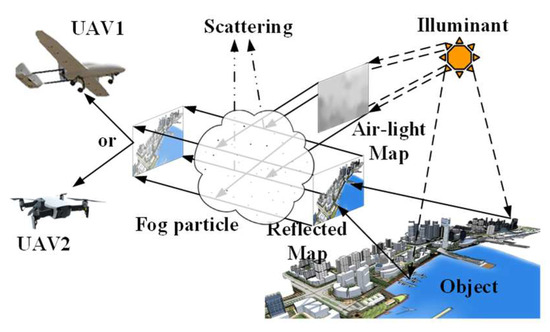
Figure 1.
The sea fog atmospheric scattering model.
3. Design of Fusion Atmospheric Light
The main effect of atmospheric light in our design is to adjust the overall brightness of the image, weaken the darkening effect caused by the attenuation of light intensity, and make the image clearer. Since the atmospheric light in a real environment cannot be collected separately due to interference from reflections, an approximate quantity can only be obtained by estimation methods. In those scenes with a small image span, the lighting environment would be similar, so many existing algorithms ignore the panoramic information and use estimated atmospheric light value to calculate a single value, which is set as the atmospheric light reference.
In the dark channel method [16], the atmospheric light value estimation method is defined as calculating the pixel mean corresponding to the brightest 0.1% pixels in the dark channel as the atmospheric light reference. The dark channel can be expressed as:
where Idark is a dark channel, x is a pixel in the image, c is any channel in RGB, and y is a pixel in the local Ω with x as the center. The estimation of atmospheric light value is:
where is the brightest 0.1% pixels in the dark channel, argtop(I) is the function that calculate the coordinate of the top 0.1% in the input I, and is the average obtained.
In Equation (3), the pixel values of the brightest 0.1% points are similar to the brightest point but the calculation cost is high. While obtaining the brightest 0.1%, we need to sort the dark channels. Therefore, in order to improve efficiency, the image pixel corresponding to the largest pixel of the dark channel is directly taken as the atmospheric light estimate, that is:
where Acs is the simplified estimation of atmospheric light value and is the largest pixel of the dark channel. Most time can be saved by using the simplified methods shown in Table 1.

Table 1.
Atmospheric light estimation process statistics.
However, the sea fog image often has a large scene span and reflection, and the atmospheric light value is not applicable to the global lighting environment, and the selection of atmospheric light value is affected by the reflective region. The use of atmospheric light value will lead to poor fog removal effect and even distortion, and the atmospheric light map cannot achieve good estimation effect due to complex scenes, etc. Therefore, this paper adopts the design scheme of atmospheric light fusion. We first simplify the calculation method of dark channel atmospheric light value, obtains a rough estimate of atmospheric light value, and then obtains the atmospheric light map through the features of the image.
In order to enhance the local characteristics of atmospheric light, we use guide filter to obtain the features with local, and the brightness channel V is selected from the image HSV space and used as the guide layer for guiding filter to described as the features of the image. The fusion atmospheric light map can be written as:
where guidedfilter() is the guide filter function [18], Iv is the brightness channel, λ is the fusion parameter to adjust the fusion radio, and 0.9 is taken in this paper.
As shown in Figure 2 and Table 1, for the original image containing fog of 950 × 617 size, the atmospheric light value of the darker channel after simplification is saved by nearly 3.5 s, and the time of atmospheric light image after fusion is still saved by nearly 2.9 s. At the same time, the average value of the atmospheric light map after fusion is darker than that of the channel to obtain the approximate atmospheric light. Additionally, the global information is richer. To sum up, the integrated atmospheric light design in this paper not only considers the global information, but also reduces the calculation time.
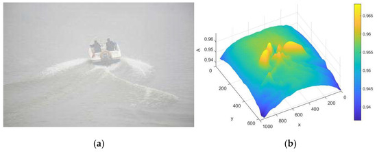
Figure 2.
Fog image and its effect of fused atmospheric light. (a) sea fog image; (b) the effect of R channel fused atmospheric light map. The X, Y axes correspond to the x, y coordinates of the image, respectively, and the Z axis denotes the atmospheric light map A.
4. The Improved Convex Optimization Model
4.1. Convex Optimization Model
Based on the Section 3. design of fusion atmospheric light, we can option the atmospheric light A faster. As Equation (1), we can calculate the clear image J, with a known t, after the atmospheric light map estimation is completed. In this section, we use convex optimization model to calculate the transmittance t.
According to the atmospheric scattering model (1), it is known that when got fog-containing image I and atmospheric light estimation A, only clear image J and transmission t are unknown. In this regard, the joint estimation of J and t can be regarded as a double-coupled problem, and J × t is considered as a whole problem set. A convex optimization model is reconstructed for model (1). We set
Therefore, according to Equations (6) and (7) the atmospheric scattering model (1) can be rewritten as:
It can be seen from the reconstructed model that the unknowns Q and t have a linear relationship, so the convex optimization model is designed as:
where R(Q, t) is a convex regularization function and Y − Q + At = 0, 0 < t ≤ 1, 0 ≤ Q is a constraint derived from Equation (8).
He et al. [24] proposed that the convex regularization function can be specified as:
where is the 2-norm, is the TV norm, and λ1, λ2, λ3 are three regularization parameters.
However, the RGB three channels in the image are independent of each other and have no correlation, so the setting of the penalty item is unreasonable. At the same time, in order to reduce the parameters and strengthen the smoothness and edge characteristics of transmission, the weight of TV norm term is set to 1, and the coefficient of 2 norm term is controlled to adjust the model performance. Therefore, the convex optimization model in this paper can be described as:
where ɑ is the regularization parameter. Therefore, combined with constraints given in Equation (9), the objective function of the convex optimization model can be written as:
where μ is the constraint parameter, which controls the influence of the constraint term on the objective function and the μ value increases with the increase in the number of iterations. In order to solve the optimal solution of this model, an improved split Bregman algorithm is designed for iteration.
4.2. Improved Split Bregman Iterative Algorithm
According to the split Bregman [32] iteration, Equation (10) can be written as:
where dx, dy are the gradients of t in the x, y directions, ∇x, ∇y are the derivatives with respect to the x, y directions. bx, by are Bregman parameters, which have the effect of accelerating convergence. We take the derivative of t in the formula and set it to zero:
Therefore, the iterative formula can be written as:
In order to improve the iteration speed, we improved the split Bregman iteration by increasing the weight of the iterative derivative term. Thus, Equation (13) can be rewritten as
Change the derivative coefficient to λ to accelerate the iteration speed.
According to Equation (16), we can obtain the transmittance t by the improved split Bregman iterative algorithm. Firstly, we set the initial parameters dx = dy = bx = by = 0. Then, we calculate Q from Equation (7) using the known fog image I and atmospheric light A. Finally, the parameters are computed iteratively. The specific iteration process pseudo-code is as follows:
In Algorithm 1, the shrink() is the shrink function which explicitly computes the optimal value [32] and it can be written as
where μ is the parameter to be shrunk and γ is the shrinking step.
| Algorithm 1. Improved split Bregman iterative algorithm | |
| 1: | Initialization: |
| dx = dy = bx = by = 0, | |
| 2: | Input: fog image I, atmospheric light A |
| Set | |
| 3: | While: > 0.001 |
| 4: | |
| 5: | |
| 6: | |
| 7: | |
| 8: | |
| 9: | End |
| 10: | Output: the transmittance t |
4.3. Algorithm Flow
According to Equation (6), the clear images can be calculated as
Combined with the fusion of atmospheric light and the improved convex optimization model, the improved split Bregman iteration is used to calculate the clear image. The whole algorithm flow is shown in Figure 3.
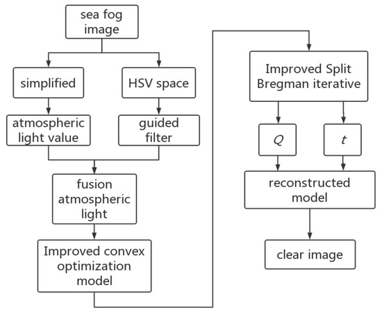
Figure 3.
Algorithm flow chart.
The specific steps are:
- Step 1:
- Calculation of fused atmosphere: the atmospheric light value is quickly obtained according to the simplified atmospheric light value estimation method, and the V channel combined with guided filtering is used to perform fused atmospheric light estimation;
- Step 2:
- The improved convex optimization model is constructed according to Equation (5), Equation (6) and Equation (12);
- Step 3:
- Using the improved split Bregman iteration to calculate the convex optimization model, the transmittance was obtained, and a clear image was obtained according to Equation (18).
5. Results
In the experiment, the results were compared with DCP [16], DehazeNet [14], FVID [22], MSW [20], CO [24] and CO-DHWT [25]. The method of combining subjective and objective evaluation is used for analysis. By calculating the quality of the image processed by the objective evaluation index analysis algorithm, information entropy and average gradient are used to evaluate the richness of information and texture in the image. The larger the value, the richer the information in the image and the more texture information. Haze concentration in the image is evaluated by FADE [26] and fuzzy coefficient [33]. The smaller the two coefficient values are, the smaller the haze concentration is.
5.1. Subjective Evaluation
Figure 4 shows the fog-containing image of a ship at sea and its restored image. It can be found that after DCP defogging, the image details are obviously restored, but the whole image is dark and there is some noise interference. The contrast effect of DehazeNet is inferior to that of DCP. The recovery effect of FVID after fog removal is poor, especially the treatment of dense fog is insufficient. MSW has a good recovery effect on important information areas, but some areas are overexposed due to the influence of spray. Fog was not effectively removed in CO restored images. The effect of CO-DHWT after defogging is improved to some extent, but it is still fuzzy. The restoration effect of this method is obviously improved, and the boat, figure, life buoy and sea wave texture in the figure are clearer, and the color is richer and more natural than other algorithms.
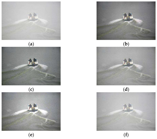
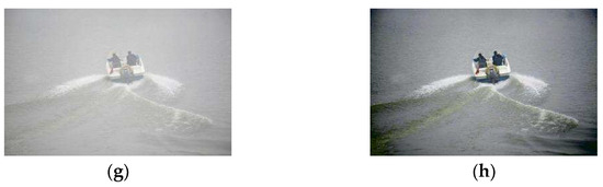
Figure 4.
Defogging effect 1. (a) sea fog image; (b) DCP; (c) DehazeNe; (d) FVID; (e) MSW; (f) CO; (g) CO-DHWT; (h) proposed method.
Figure 5 shows the fog-containing image of the coastal landscape and its restored image, including coastal buildings and cruise ships. The color of DCP after fog removal is dark, not rich enough, and there is a certain halo effect. DehazeNet is more natural after removing the fog, but the details are not prominent enough. The effect of FVID after fog removal is insufficient, the image details are not greatly improved, and the whole is dark. The detail of MSW is more prominent than other algorithms, but the halo is more obvious. The effect of CO and CO-DHWT after defogging is not obvious, and both contain obvious fog. The color and details of the image after fog removal are more prominent than other algorithms, and the visual perception is more natural.
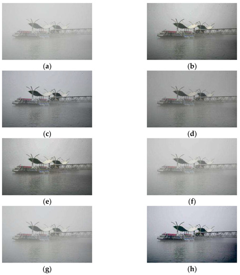
Figure 5.
Defogging effect 2. (a) sea fog image; (b) DCP; (c) DehazeNe; (d) FVID; (e) MSW; (f) CO; (g) CO-DHWT; (h) proposed method.
Figure 6 shows the fog image and its restoration image of sea surface monitoring, including two distant ship targets. After DCP treatment, there was obvious halo phenomenon in the sky area. After DehazeNet treatment, the effect was not obvious, and the distant target was not clear enough. After FVID treatment, the overall brightness decreased significantly and the detail restoration was insufficient. MSW processing distant objects are not prominent, the details of the texture is not prominent. The effect of CO and CO-DHWT treatment is obviously not ideal, and the target texture is not well restored. After processing, the two distant objects and the texture of the sea surface are more clearly visible, and the effect is obviously better than above algorithms [14,16,20,22,24,25].
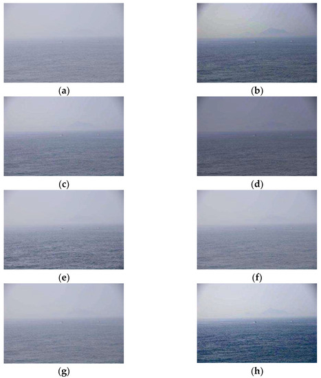
Figure 6.
Defogging effect 3. (a) sea fog image; (b) DCP; (c) DehazeNe; (d) FVID; (e) MSW; (f) CO; (g) CO-DHWT; (h) proposed method.
Figure 7 shows the fog-containing images of coastal buildings and their restoration images. After DCP treatment, the fog was effectively eliminated for the building groups including artificial islands, coastal roads, Bridges, etc., but the whole was dark and the color was not clear. After DehazeNet processing, the near scene is improved, but the distant scene is fuzzy and the processing effect is not obvious. After FVID processing, the texture details are not prominent enough and the overall sense of hierarchy is lacking. After MSW treatment, the color is not natural, and there is halo phenomenon in the sky area. The effect of CO and CO-DHWT on the fog area is not obvious, and the distant objects are blurred. However, after the processing of our proposed algorithm, the color of the image is obviously richer and the architectural texture becomes clearer.
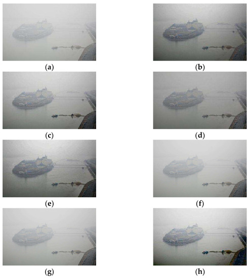
Figure 7.
Defogging effect 4. (a) sea fog image; (b) DCP; (c) DehazeNe; (d) FVID; (e) MSW; (f) CO; (g) CO-DHWT; (h) proposed method.
5.2. Objective Evaluation
According to the experimental results in Figure 8 and Table 2, after DCP treatment, the information entropy and average gradient are improved, but the brightness is low and the color is not rich enough, and the contrast is significantly reduced. The training dataset of DehazeNet is an artificial indoor synthetic haze image, and the processing effect of real fog is insufficient, so the performance of all objective parameters is not outstanding. The average gradient of FVID is improved, but the information entropy and contrast are not improved enough, and the defogging effect is limited. The processing of texture details is obviously better in MSW, and the average gradient and FADE are significantly improved, which is better than other algorithms, but the information entropy is not significantly improved. However, the information entropy, average gradient, FADE, and fuzzy coefficient data of the proposed algorithm are all better, and the haze concentration of the restored image is significantly reduced, and the fog removal effect is obvious.
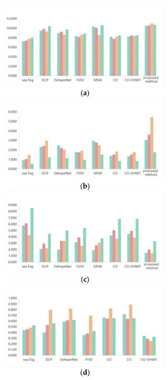
Figure 8.
The objective evaluation index. (a) information entropy; (b) average gradient; (c) FADE; (d) fuzzy coefficient.
Table 2.
The objective evaluation index.
6. Conclusions
In this paper, we introduce an improved convex optimization model for the aerial station captured sea fog images to implement effectively defogging. In view of the complex information and rich details in aerial sea images, we propose a design for a fusion atmospheric light map, which is different from the traditional solutions that directly use the obtained atmospheric light value. The solution of simplifying atmospheric light value estimation and the V channel of HSV space through fusion process also saves computation time compared with the DCP method, while it obtains more local information. To reduce reliance on prior conditions, we show the improved convex optimization methods derived by the atmospheric scattering model. Moreover, the improved split-Bregman iterative method is proposed to obtain transmittance and a clear image. Our experimental results indicate that the detailed texture and color of the image are effectively restored using our methods. The overall image is clearer and more natural than that using traditional methods. Meanwhile, the objective indexes of the proposed algorithm, such as information entropy, average gradient, FADE and fuzzy coefficient, achieve their optimal results. Therefore, this paper provides an effective defogging method for sea fog images, and a feasible scheme for defogging in complex sea environments. Our method can make the object in the restored sea fog image clearer and more realistic with rich details than traditional methods. In the future, it could facilitate the study of marine vision problems, such as target detection and monitoring systems in complex marine scenes.
Author Contributions
Conceptualization, H.H. and M.N.; methodology, Z.L.; software, Z.L.; validation, M.N., H.H. and Z.L.; formal analysis, M.S.M.; investigation, M.N. and H.W.; resources, T.G.; data curation, H.H.; writing—original draft preparation, Z.L.; writing—review and editing, M.N.; visualization, Z.L.; supervision, M.N.; project administration, H.H.; funding acquisition, M.N. All authors have read and agreed to the published version of the manuscript.
Funding
This research was supported by the General projects of the National Natural Science Foundation of China, grant number 52172379, 52172324, the Project of the Ministry of Science and Technology of China, grant number G2021171024L, the Fundamental Research Funds for the Central Universities, CHD, grant number 300102323501, and the Open Fund project of Xi’an Key Laboratory of Intelligent Expressway Information Fusion and Control (Chang’an University), grant number 300102323502.
Institutional Review Board Statement
Not applicable.
Informed Consent Statement
Not applicable.
Data Availability Statement
Not applicable.
Conflicts of Interest
The authors declare no conflict of interest.
References
- Zhang, Z.; Cai, L.; Li, Z. A Novel Sea Fog Image Enhancement Method Based on Dark Channel Prior and Improved Transmission Model. Remote Sens. 2022, 14, 967. [Google Scholar]
- Li, Z.; Zhu, Z.; Gao, M.; Zhou, H. Improved dehazing method for remote sensing images based on dark channel prior. Remote Sens. 2020, 12, 3193. [Google Scholar] [CrossRef]
- Rolly, R.M.; Malarvezhi, P.; Lagkas, T.D. Unmanned aerial vehicles: Applications, techniques, and challenges as aerial base stations. Int. J. Distrib. Sens. Netw. 2022, 18, 9:1–9:24. [Google Scholar] [CrossRef]
- Abualigah, L.; Diabat, A.; Sumar, P.; Gandomi, A.H. Applications, Deployments, and Integration of Internet of Drones (IoD): A Review. IEEE Sens. J. 2021, 21, 25532–25546. [Google Scholar] [CrossRef]
- Wang, D.; Wu, M.; Wei, Z.; Yu, K.; Min, L.; Mumtaz, S. Uplink Secrecy Performance of RIS-based RF/FSO Three-Dimension Heterogeneous Networks. IEEE Trans. Wirel. Commun. 2023. early access. [Google Scholar] [CrossRef]
- Jin, G.Q.; Gao, S.H.; Shi, H.; Lu, X.; Yang, Y.; Zheng, Q. Impacts of Sea-Land Breeze Circulation on the Formation and Development of Coastal Sea Fog along the Shandong Peninsula: A Case Study. Atmosphere 2022, 13, 165. [Google Scholar] [CrossRef]
- Wang, D.; He, T.; Lou, Y.; Pang, L.; He, Y.; Chen, H.H. Double-edge Computation Offloading for Secure Integrated Space-air-aqua Networks. IEEE Internet Things J. 2023, 10, 15581–15593. [Google Scholar] [CrossRef]
- Huang, H.; Hu, K.Y.; Guo, L.; Wang, H.F.; Zhu, L.Y. Improved defogging algorithm for sea fog. J. Harbin Inst. Technol. 2021, 53, 81–91. (In Chinese) [Google Scholar] [CrossRef]
- Singh, D.; Kumar, V. Single image haze removal using integrated dark and bright channel prior. Mod. Phys. Lett. B 2018, 32, 1850051. (In Chinese) [Google Scholar] [CrossRef]
- Fattal, R. Single image dehazing. In Proceedings of the ACM SIGGRAPH Conference 2008, Singapore, 11–15 August 2008. [Google Scholar] [CrossRef]
- Wang, D.; He, T.; Zhou, F.; Cheng, J.; Zhang, R.; Wu, Q. Outage-driven link selection for secure buffer-aided networks. Sci. China Inf. Sci. 2022, 65, 182303. [Google Scholar] [CrossRef]
- Hwang, B.M.; Lee, S.H.; Lim, W.T.; Ahn, C.B.; Son, J.H.; Park, H. A fast spatial-domain terahertz imaging using block-based compressed sensing. J. Infrared Millim. Terahertz Waves 2011, 32, 1328–1336. [Google Scholar] [CrossRef]
- Herman, M.A.; Strohmer, T. High-resolution radar via compressed sensing. IEEE Trans. Signal Process. 2009, 57, 2275–2284. [Google Scholar] [CrossRef]
- Cai, B.L.; Xu, X.M.; Jia, K.; Qing, C.M.; Tao, D.C. DehazeNet: An End-to-End System for Single Image Haze Removal. IEEE Trans. Image Process. 2016, 25, 5187–5198. [Google Scholar] [CrossRef] [PubMed]
- Qin, X.; Wang, Z.L.; Bai, Y.C.; Xie, X.D.; Jia, H.Z. FFA-Net: Feature fusion attention network for single image dehazing. In Proceedings of the AAAI Conference on Artificial Intelligence, New York, NY, USA, 7–12 February 2020. [Google Scholar] [CrossRef]
- He, K.M.; Sun, J.; Tang, X.O. Single Image Haze Removal Using Dark Channel Prior. IEEE Trans. Pattern Anal. Mach. Intell. 2011, 33, 2341–2353. [Google Scholar] [CrossRef]
- Han, H.N.; Qian, F.; Zhang, B. Single-image dehazing using scene radiance constraint and color gradient guided filter. Signal Image Video Process. 2022, 16, 1297–1304. [Google Scholar] [CrossRef]
- Guo, Z.Y.; Yu, X.T.; Du, Q.L. Infrared and visible image fusion based on saliency and fast guided filtering. Infrared Phys. Technol. 2022, 123, 104178. [Google Scholar] [CrossRef]
- Yuan, Y.; Zheng, J.; Gong, X. Sea fog image enhancement algorithm based on adaptive guided filtering. IOP Conf. Ser. Earth Environ. Sci. 2020, 551, 012019. [Google Scholar] [CrossRef]
- Huang, H.; Li, X.R.; Song, J.; Wang, H.F.; Ru, F.; Sheng, G.F. A traffic image dehaze method based on adaptive transmittance estimation with multi-scale window. Chin. Opt. 2019, 12, 1311–1320. (In Chinese) [Google Scholar] [CrossRef]
- Zhu, Q.S.; Mai, J.M.; Shao, L. A Fast Single Image Haze Removal Algorithm Using Color Attenuation Prior. IEEE Trans. Image Process. 2015, 24, 3522–3533. [Google Scholar] [CrossRef]
- Galdran, A.; Vazquez-Corral, J.; Pardo, D.; Bertalmio, M. Fusion-based variational image dehazing. IEEE Signal Process. Lett. 2017, 24, 151–155. [Google Scholar] [CrossRef]
- Ling, P.; Chen, H.; Tan, X.; Jin, Y.; Chen, E. Single Image Dehazing Using Saturation Line Prior. IEEE Trans. Image Process. 2023, 32, 3238–3253. [Google Scholar] [CrossRef] [PubMed]
- He, J.X.; Zhang, C.S.; Yang, R.; Zhu, K. Convex optimization for fast image dehazing. In Proceedings of the IEEE International Conference on Image Processing, Phoenix, AZ, USA, 25–28 September 2016. [Google Scholar] [CrossRef]
- He, J.X.; Xing, F.Z.; Yang, R.; Zhang, C.S. Fast Single Image Dehazing via Multilevel Wavelet Transform based Optimization. arXiv 2019, arXiv:1904.08573. [Google Scholar]
- Choi, L.K.; You, L.; Bovik, A.C. Referenceless Prediction of Perceptual Fog Density and Perceptual Image Defogging. IEEE Trans. Image Process. 2015, 24, 3888–3901. [Google Scholar] [CrossRef] [PubMed]
- McCartney, E.J. Optics of the Atmosphere: Scattering by Molecules and Particles. Phys. Today 1977, 30, 76–77. [Google Scholar] [CrossRef]
- Narasimhan, S.G.; Nayar, S.K. Contrast restoration of weather degraded images. IEEE Trans. Pattern Anal. Mach. Intell. 2003, 25, 713–724. [Google Scholar] [CrossRef]
- Gao, M.; Zhu, X.; Li, Z.; Yu, L. Improved sea fog image dehazing algorithm based on multi-channel transmission estimation. J. Vis. Commun. Image Represent. 2021, 75, 103109. [Google Scholar]
- Li, L.; Du, X.; Yang, F. Improved sea fog image enhancement method based on local atmospheric light estimation. Sensors 2021, 21, 1077. [Google Scholar] [CrossRef]
- Huang, H.; Li, Z.Y.; Hu, K.Y.; Wang, H.F.; Ru, F.; Wang, J. UAV aerial image dehazing by fusion of atmospheric light value and graph estimation. J. Harbin Inst. Technol. 2023, 55, 88–97. (In Chinese) [Google Scholar] [CrossRef]
- Goldstein, T.; Osher, S. The Split Bregman Method for L1-Regularized Problems. SIAM J. Imaging Sci. 2009, 2, 323–343. [Google Scholar] [CrossRef]
- Huang, H.; Hu, K.Y.; Song, J.; Wang, H.F.; Ru, F.; Guo, L. A twice optimization method for solving transmittance with haze-lines. J. Xi’an Jiaotong Univ. 2021, 55, 130–138. (In Chinese) [Google Scholar]
Disclaimer/Publisher’s Note: The statements, opinions and data contained in all publications are solely those of the individual author(s) and contributor(s) and not of MDPI and/or the editor(s). MDPI and/or the editor(s) disclaim responsibility for any injury to people or property resulting from any ideas, methods, instructions or products referred to in the content. |
© 2023 by the authors. Licensee MDPI, Basel, Switzerland. This article is an open access article distributed under the terms and conditions of the Creative Commons Attribution (CC BY) license (https://creativecommons.org/licenses/by/4.0/).