Article

A Fuzzy Dempster–Shafer Evidence Theory Method with Belief Divergence for Unmanned Surface Vehicle Multi-Sensor Data Fusion

1
College of Marine Electrical Engineering, Dalian Maritime University, Dalian 116026, China
2
Key Laboratory of Technology and System for Intelligent Ships of Liaoning Province, Dalian 116026, China
*
Author to whom correspondence should be addressed.
J. Mar. Sci. Eng. 2023, 11(8), 1596; https://doi.org/10.3390/jmse11081596
Submission received: 19 July 2023 / Revised: 11 August 2023 / Accepted: 12 August 2023 / Published: 15 August 2023
(This article belongs to the Special Issue Advances in Sensor Technology in Smart Ships and Offshore Facilities)

Abstract

:
The safe navigation of unmanned surface vehicles in the marine environment requires multi-sensor collaborative perception, and multi-sensor data fusion technology is a prerequisite for realizing the collaborative perception of different sensors. To address the problem of poor fusion accuracy for existing multi-sensor fusion methods without prior knowledge, a fuzzy evidence theory multi-sensor data fusion method with belief divergence is proposed in this paper. First of all, an adjustable distance for measuring discrepancies between measurements is devised to evaluate the degree of measurement closeness to the true value, which improves the adaptability of the method to different classes of sensor data. Furthermore, an adaptive multi-sensor measurement fusion strategy is designed for the case where the sensor accuracy is known in advance. Secondly, the affiliation function of the fuzzy theory is introduced into the evidence theory approach to assign initial evidence of measurements in terms of defining the degree of fuzzy support between measurements, which improves the fusion accuracy of the method. Finally, the belief Jensen–Shannon divergence and the Rényi divergence are combined for measuring the conflict between the evidence pieces to obtain the credibility degree as the reliability of the evidence, which solves the problem of high conflict between evidence pieces. Three examples of multi-sensor data fusion in different domains are employed to validate the adaptability of the proposed method to different kinds of multi-sensors. The maximum relative error of the proposed method for multiple sensor experiments is greater than or equal to 0.18%, and its error accuracy is much higher than the best result of 0.46% among other comparative methods. The experimental results verify that the proposed data fusion method is more accurate than other existing methods.

1. Introduction

Unmanned surface vehicles (USVs) have received increasing attention as a novel platform for widespread application in the marine environment [1,2], e.g., depth measurement, water quality detection and environmental monitoring, etc. The application of USVs in these fields relies on the perception capability of the sensors, and the accuracy of the measurement information is crucial in determining whether the parameters to be detected fulfill the detection requirements [3]. The information collected by a single sensor is often not guaranteed to be comprehensive, reliable and high-performance, so multiple sensors are required to be involved in the measurement to ensure that more accurate parameter information is obtained [4]. The measurements collected by multiple sensors can only be fused to obtain more accurate results, and the multi-sensor data fusion technology is an essential means of achieving data fusion, which has led to a wide range of applications in integrated navigation [5], target tracking [6], fault diagnosis [7], position control [8], dynamic positioning [9] and path following [10], etc.
To obtain more reliable measurements and higher fusion accuracy, numerous multi-sensor data fusion methods [11,12,13] suitable for different situations have been proposed. The adaptive weighted fusion method is a relatively simple method that assigns an optimal weighting factor to each sensor according to the principle of mean square error minimization [14]. The Bayesian approach computes the posterior probability of the target based on Bayes’ law and has a high fusion accuracy [15]. The Kalman filter, based on the statistical properties of the system model, is used for data fusion estimation by recursive operations [16]. The fuzzy logic inference method can utilize the experience of experts as a guide for improving the accuracy and anti-interference of the system by adopting an effective fusion scheme [17]. The artificial neural network data fusion method can effectively reduce redundant data transmission to increase the real-time efficiency and accuracy of data fusion and improve the performance of the data fusion method [18]. A multi-sensor data fusion method based on reinforcement learning has been proposed to obtain the fusion result, which utilizes the error between the fused value and the actual value to achieve enhancement of the fusion accuracy [19]. A sparse-grid quadrature filtering distributed state fusion method has been proposed to address the multi-sensor nonlinear system’s fusion estimation problem, where the measurements from each sensor are processed by the sparse-grid orthogonal filtering in a distributed form and fused using the cross-covariance method [20]. A discrete factor data fusion method has been proposed for multi-sensor target identification, where the measurements collected by multiple sensors construct discrete factors corresponding to sensor and target characteristics to assign multi-sensor weights, which establishes the correlation and relative consistency of multiple sensors [21]. To extract discriminative characteristics from multi-sensor measurements for accurate diagnosis, a novel multi-task multi-sensor fusion network has been proposed to enhance the performance of fault diagnosis [22]. To solve the optimal state estimation problem that minimizes the noise-induced error, a recursive algorithm that fuses multiple sensor measurements to calculate the system state prior and posterior beliefs has been proposed according to the algebraic form of the stochastic Boolean network and Bayes’ law [23]. To solve the problem of decreasing accuracy and reliability of multi-sensor measurements due to occasional sensor failures and environmental perturbations, a game-theory-based data fusion method is proposed, which uses data-driven adaptive weighted fusion and model-driven discrete Kalman fusion as the game objectives for real-time estimation of the ship’s heading and position to design a game strategy for the fusion of measurements [24]. However, these methods cannot be used, or have poor fusion performance, without any prior information.

Related Work

The Dempster–Shafer (D–S) evidence theory has been the subject of a great deal of extensive and in-depth research as an easy way to solve the problem of uncertainty without prior information [25,26]. The focus of this research is its application to multi-sensor data fusion, which produces counter-intuitive results when highly conflicting evidence is encountered [27]. To solve the counterintuitive problem caused by highly conflicting evidence, a symmetric fractal-based belief Kullback–Leibler divergence has been proposed to measure the conflict between evidence pieces, and a new data fusion algorithm has been devised to apply the belief Kullback–Leibler difference measure to practical problems [28]. To address the problem of highly conflicting evidence leading to a series of counterintuitive results, a novel D–S evidence theory confidence divergence measure has been proposed, which integrates the mass function’s confidence measure and likelihood measure, and a new multi-source data fusion method has been proposed [29]. To solve the problem that Dempster’s combination rule leads to unreasonable results in fusing highly conflicting evidence, a novel Tanimoto measure-based evidence similarity measure method has been proposed to describe the inconsistency between evidence subjects [30]. To address the issue that the D–S evidence theory combination method cannot be used when the evidence is highly conflicting, a reward and trust allocation mechanism has been proposed based on the principle of mutual trust between basic probability assignments (BPAs), which enhances the conflicting evidence fusion’s convergence [31]. To deal with the counterintuitive problem that may occur when handling highly conflicting evidence, a modified evidence theory method has been proposed to design a new distribution distance measure for measuring the conflict of evidence pieces with each other and, thus, obtain the credibility of the evidence [32]. To deal with highly conflicting evidence, a new divergence measure has been presented for evaluating the distance between evidence pieces, while a multi-source data fusion method that takes into account the mutual supportiveness and uncertainty of the evidence was developed [33]. To exploit the essential implicit information behind the evidence pieces, a new conflict evidence combination method has been proposed, which considers the similarity of the evidence pieces to define the composite credibility [34]. However, these multi-sensor data fusion methods are generally used in fields such as fault diagnosis and target identification, and they do not fuse measurements collected by multiple sensors. To solve the problem of poor accuracy of multi-sensor data fusion, an improved evidence theory multi-sensor data fusion method has been proposed to realize the fusion of measurements collected by multi-sensors by assigning weights to each piece of evidence based on the degree of support between measurements [35]. To further improve the accuracy of existing multi-sensor data fusion methods and to cope with situations where the sensor accuracy is known, in this paper, a fuzzy evidence theory multi-sensor data fusion method with belief divergence is proposed based on [35]. The major contributions of this paper are as follows:
(1)
An adjustable distance for measuring discrepancies between measurements is devised to evaluate the closeness of the measured values to the true value, which improves the adaptability of the method to different classes of sensor data. Furthermore, an adaptive multi-sensor measurement fusion strategy is designed for the case where the sensor accuracy is known in advance.
(2)
The affiliation function of the fuzzy theory that more accurately measures the mutual support between measurements is introduced into the evidence theory approach for assigning initial evidence for each measurement, which improves the multi-sensor data fusion accuracy of the method.
(3)
The conflict between evidence pieces is measured by combining the belief Jensen–Shannon divergence and the Rényi divergence to obtain credibility of the reliability of the evidence, which mitigates the conflict of evidence to improve the multi-sensor data fusion accuracy of the method.
The rest of this paper is arranged as follows: Section 2 presents the fundamentals that will be involved in the follow-up. The main components of the proposed multi-sensor data fusion method are introduced in Section 3. A description of the testing of other existing comparative methods and the proposed method by multiple multi-sensor measurement experiments to verify the effectiveness of these methods and the superiority of the proposed method is provided in Section 4. In Section 5, the conclusions are provided.

2. Preliminaries

The fundamentals of D–S evidence theory, the Jensen–Shannon divergence, and the Rényi divergence are briefly introduced in this section.

2.1. D–S Evidence Theory

D–S evidence theory, an uncertain reasoning method and belief function theory that can effectively express and process uncertain information, has been widely used in many fields [36,37]. The concept of D–S evidence theory is introduced below.
Definition 1. 
Frame of discernment.
Let Ω be a finite number of collective non-empty and mutually exclusive events, called the discernment frame, which can be defined as
Ω = { E 1 , E 2 , , E i , E N }
The power set of Ω denoted by 2 Ω is given as follows
2 Ω = { , { E 1 } , { E 2 } , , { E N } , { E 1 , E 2 } , , { E 1 , E 2 , , E i } , , Ω }
where ∅ represents the empty set [38].
Definition 2. 
Mass function.
Given a discernment frame Ω, the mass function is defined as the mapping of 2 Ω to [ 0 , 1 ] as follows
m : 2 Ω [ 0 , 1 ]
which is constrained as
A 2 m ( A ) = 1 m ( ) = 0
where A represents the subset of 2 Ω .
Definition 3. 
Dempster’s combination rule.
Suppose there are two BPAs, m 1 and m 2 , in Ω, whose combination rule can use the orthogonal product form, i.e., m = m 1 m 2 [39]. Its particular format is described as
m ( A ) = 1 1     K A 1 A 2 = A m 1 ( A 1 ) + m 2 ( A 2 ) , A 0 , A =
where A 1 and A 2 denote the focal elements of m 1 and m 2 . K represents the conflict measure parameter for m 1 and m 2 and is written as
K = A 1 A 2 = m 1 ( A 1 ) m 2 ( A 2 )
The larger the value of K, the greater the conflict between two BPAs, and the smaller the value of K, the smaller the conflict between two BPAs [40]. It is essential to point out that Dempster’s combination rule is feasible when K < 1 .

2.2. Belief Jensen–Shannon Divergence

D–S evidence theory is characterized by the treatment of uncertain information, and the measure of conflict between evidence pieces is the key for it to possess its properties. Divergence, as an effective mathematical tool in measuring discrepancies between evidence pieces, has been widely used in many fields [41]. Numerous divergence measures have emerged in recent years, e.g., J-divergence [42], Jensen–Shannon (JS) divergence, and BRE divergence [43], etc. It differs from other divergence measures in that JS divergence does not require the condition that the associated probability distribution has absolute continuity. Based on the JS divergence, a new belief JS divergence (BJS) [44] is proposed, which may be defined below.
Definition 4. 
Belief Jensen–Shannon Divergence.
Given two independent BPAs, m 1 and m 2 , in the same discernment frame Ω, let A i be a focal element in m, which includes N mutually exclusive hypotheses. The BJS divergence for measuring the difference between m 1 and m 2 is expressed as
B J S ( m 1 , m 2 ) = 1 2 H m 1 , m 1 + m 2 2 + H m 2 , m 1 + m 2 2
where H ( m 1 , m 2 ) = m 1 ( A i ) log m 1 ( A i ) m 2 ( A i ) [45]. Its main properties are
(1) 
Symmetry: B J S ( m 1 , m 2 ) = B J S ( m 2 , m 1 ) .
(2) 
Boundary: 0 B J S ( m 1 , m 2 ) 1 .
(3) 
Triangle inequality: B J S ( m 1 , m 2 ) + B J S ( m 1 , m 3 ) B J S ( m 2 , m 3 ) .
The BJS divergence expands the JS divergence, and the BJS divergence degenerates to the JS divergence when all the subset’s BPAs are zero.

2.3. Rényi Divergence

In the field of multi-sensor data fusion, the Rényi divergence has a significant effect on either parametric or non-parametric models in the convergence of the minimum description length and proof of Bayesian estimation [46]. Rényi divergence can be described as:
Definition 5. 
Rényi divergence.
Let any sequence be α, the Rényi divergence of α from the probability distribution P = ( p 1 , , p η ) to Q = ( q 1 , , q η ) is written as
D α ( P | | Q ) = 1 α 1 ln i = 1 η p i α q i 1 α
where α ( 0 , 1 ) ( 1 , ) . If α > 1 , the rule will be adopted, i.e., 0 / 0 = 0 and x x 0 0 = ( x > 0 ) [47].

3. The Proposed Method

N sensors in the system are used to measure the parameter to be measured, and the real-time data of the single measurement of the kth sensor are Z k ( k = 1 , 2 , , N ) . Based on the core idea of evidence theory, the measurements { Z 1 , Z 2 , , Z N } of all sensors can be considered as a discriminative frame Ω . The evidence theory describes discrepancies between elements by defining basic belief assignment, converting each measurement into evidence on the discriminative frame Ω , respectively. Subsequently, the generated evidence pieces are combined, and the basic belief assignment of each measurement in the synthetic evidence is considered as the fusion weighting factor. Finally, these measurements are weighted and summed to obtain the fusion result of this data set.
The proposed method mainly comprises four components: selection of the affiliation function, basic belief assignment for measurements based on sensor credibility, conflicting measure and evidence synthesis, and evidence combination. The affiliation function of fuzzy theory can be used to yield initial evidence pieces that may indicate the degree of mutual support of measurements. The basic belief assignment can adjust initial evidence pieces based on discrepancies between measurements for assigning relatively reasonable weights to each measurement. The conflicting measure and evidence synthesis can be used to measure conflict and differences between evidence pieces to synthesize the weighted average evidence. The weighted average evidence and the corrected evidence pieces are combined to achieve multi-sensor data fusion via the evidence combination rule.

3.1. Selection of the Affiliation Function

These sensors may be a variety of active or passive detectors that measure different characteristic parameters, such as the USV state, surrounding environment information, target state, equipment wear and tear, and control system parameters, respectively. Since the measurements are subject to measurement error, environmental noise and human interference and other factors, the measurements collected by each sensor comprise different results, but the measurements can be regarded as the superposition of the true value of the parameters and the noise. From a qualitative perspective, all measurements within the normal deviation range should fall in the neighborhood of the true value. The affiliation function of the measurements obtained by the kth sensor is expressed as
φ i j = 1 2 arctan Z i Z j π
where Z i and Z j denote the ith and jth sensor’s measurements, respectively.
φ i j indicates the extent to which the measured value of the ith sensor deviates from that of the jth sensor. Intuitively, if φ i j is large, i.e., the measurement Z i deviates significantly from the true value of the parameter to be measured, then the probability that the measurement of the ith sensor belongs to the true value is considered to be low. Conversely, if φ i j is very small, i.e., the measurement Z i is very close to the true value of the parameter, then the probability that the measurement of the ith sensor belongs to the true value is considered to be high.
For the discernment frame Ω , the affiliation matrix of each sensor for the parameters to be measured is
U i j = φ 11 φ 12 φ 1 N φ 21 φ 22 φ 2 N φ N 1 φ N 2 φ N N
If the accuracy information σ j ( j = 1 , 2 , , N ) of each sensor is known in advance, the affiliation matrix needs to be further adjusted. Considering the relationship between the prior accuracy information of each sensor and the affiliation matrix, the initial evidence pieces can be adjusted as follows
U i j = ( 1 / σ j 2 ) U i j , i , j = 1 , 2 , , N
The affiliation matrix reflects the degree to which all sensor measurements support each other, which corresponds to the probability that the measurement is close to the true value. It can be considered as the initial evidence of the measurements to provide initial values for subsequent corrections of the evidence.

3.2. Basic Belief Assignment for Measurements Based on Sensor Credibility

In the practical environment, the measurement of each sensor may be unreliable due to various disturbances. Large deviations or even wrong information may appear in the measurements, which can affect the accuracy of data fusion or even lead to wrong fusion results. To improve the fusion accuracy, it is necessary to check the consistency of the multi-sensor measurements and to fuse the confidence of the sensor measurements into the evidence assignment. To reflect the magnitude of the deviation between different sensor measurements, it can be determined by the measurements themselves. The distance between the measurements of N sensors is written as
d i j = Z i Z j λ
where i , j = 1 , 2 , , N , λ is a factor that moderates the degree of variation between measurements. The introduction of λ enables the method to select different λ for different types of multi-sensor measurements to reflect more effectively in terms of the degree of support between measurements, which facilitates the reasonable generation of evidence. The average distance d i from measurement Z i to each measurement is given as follows:
d i = j = 1 , i j N d i j N 1
The magnitude of d i indicates the degree of difference between sensor i and the remaining sensors. The smaller d i is, the smaller the difference between sensor i and the remaining sensors, which is considered as a high degree of mutual support and credibility between them. Conversely, it indicates that the sensor singularity is serious and the credibility of the sensor is low. The average distance between the entire measurements can be given by
d ¯ = i = 1 N d i N
where z j 1 and z j 2 denote any two valid measurements, and α is a threshold that satisfies α 1 [48].
Based on the evaluation of the credibility of each sensor, a basic belief assignment method is used to convert the measurements into evidence. Its core idea is to consider the obtained affiliation matrix as the initial evidence of the measurements and to correct the initial evidence by using the distance between the measurements as the measure of the probability that the measurements are close to the true value. If d i > d ¯ , the sensor’s measurement has a large deviation and is rejected. Conversely, the measurement is valid. The correction formula is described as
m i ( Z j ) = 0 , d j > τ d ¯ m i ( Z j 1 ) m i ( Z j 2 ) = d j 2 d j 1 , d j τ d ¯
where Z j 1 and Z j 2 are two arbitrary valid measurements, and τ 1 represents the threshold.
In the actual operation, a group of credibility correction factors for the initial evidence can be produced from (15), and the correction factors are utilized for normalizing and weighting the initial evidence, i.e.,
m i ( Z j ) = ω j m i ( Z j ) p = 1 N ω p m i ( Z p )
If the accuracy information of each sensor is known in advance, the fusion weights need to be further adjusted. To improve the robustness of the fusion method, the prior accuracy information of each sensor and the weight assignment strategy need to be considered comprehensively [49]. The additional correction factors can be obtained as
v i = 1 σ i 2 k = 1 N 1 σ i 2
The additional correction factors are utilized for normalizing and weighting the evidence, i.e.,
m i ( Z j ) = v j m i ( Z j ) s = 1 N v s m i ( Z s )

3.3. Conflicting Measure and Evidence Synthesis

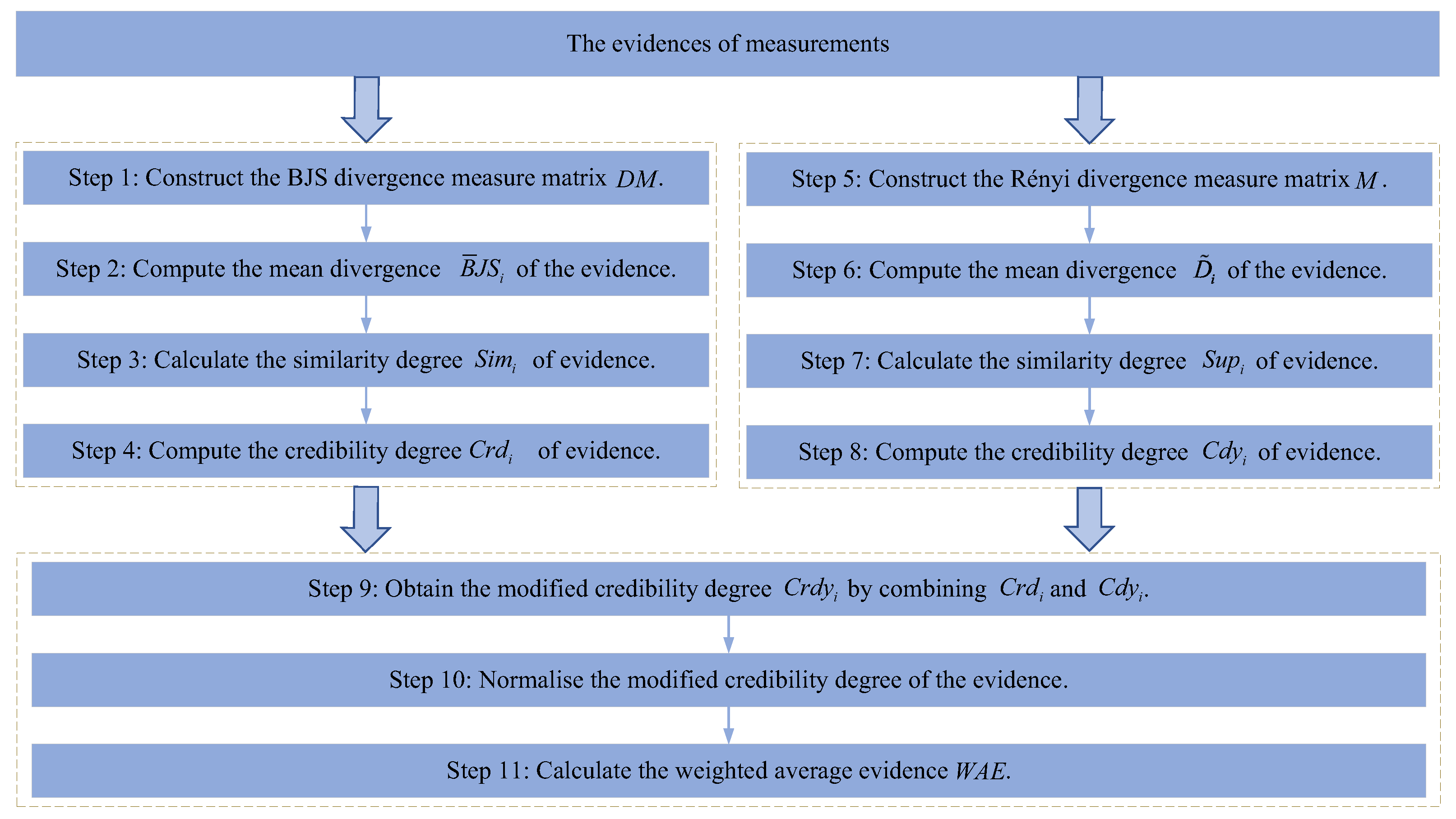
This section mainly considers the BJS divergence and the Rényi divergence. Firstly, the BJS divergence is used for measuring the degree of conflict and discrepancy between evidence pieces and the credibility, i.e., the reliability of the evidence is obtained through the BJS divergence measure [44]. Secondly, the Rényi divergence is also used for measuring the degree of conflict between the evidence pieces to obtain credibility. Finally, two kinds of divergence can be combined and normalized to form the final evidence, which is synthesized with the existing evidence as the latest piece of evidence to participate in the final evidence synthesis. A flowchart for the conflicting measure and evidence synthesis is shown in Figure 1, which involves the following steps:
Step 1: In accordance with (7), the BJS divergence between any two pieces of evidence m i and m j is calculated and described as B J S i j . The divergence measure matrix D M can be given by [33]:
D M = 0 B J S 1 i B J S 1 N B J S i 1 0 B J S i N B J S N 1 B J S N i 0
Step 2: The mean divergence distance of the evidence m i based on the D M is obtained as follows
B ¯ J S i = j = 1 , j i N B J S i j N 1
Step 3: The similarity degree for the evidence m i can be given by
S i m i = 1 B ¯ J S i
Step 4: The degree of credibility for the evidence m i can be written as
C r d i = S i m ( m i ) j = 1 N S i m ( m j )
Step 5: In accordance with (8), the Rényi divergence between any two pieces of evidence m i and m j is calculated and described as D i j . The divergence measure matrix M can be given by
M = 0 D 1 i D 1 N D i 1 0 D i N D N 1 D N i 0
Step 6: The mean divergence distance of the evidence m i based on the M is obtained as follows
D ˜ i = j = 1 , j i N D i j N 1
Step 7: The support degree for the evidence m i can be given by
S u p i = 1 D ˜ i
Step 8: The degree of credibility for the evidence m i can be written as
C d y i = S u p ( m i ) j = 1 N S u p ( m j )
Step 9: C r d i and C d y i are combined to take advantage of both and are described as follows
C r d y i = C r d i × C r y i
Step 10: The modified credibility degree is normalized as the final weight of each piece of evidence m i , which is expressed as
C ˜ r d y i = C r d y i j = 1 N C r d y j
Step 11: According to C ˜ r d y i , the weighted average evidence W A E is given as a new piece of evidence as follows
W A E i = i = 1 N ( C ˜ r d y i × m i )

3.4. Evidence Combination

There may be a high degree of conflict between the N pieces of evidence generated by (10) to (18), so Dempster’s combination rule may yield unreasonable combination results, leading to unreasonable weight assignments of the measurements. Since the evidence combination rule of [39] can effectively alleviate the above problems and assign a more reasonable weight to the measurement, we adopt this rule.
The probability of support for the conflict between evidence pieces is proportionally allocated to each measurement, and its combined form is expressed as follows
m ( Z j ) = i = 1 N m i ( Z j ) + e m ¯ i ( Z j )
where m ¯ i ( Z j ) represents the average basic belief assignment of Z j across evidence pieces. The conflict factor e can be given by
e = 1 j = 1 N i = 1 N m i ( Z j )
m ¯ i ( Z j ) can be written as
m ¯ i ( Z j ) = 1 N i = 1 N m i ( Z j )
The m ( Z j ) of Z j among the synthetic evidence pieces are the weights obtained by Z j . Then the fusion result is given by
Z 0 = j = 1 N Z j m ( Z j )
The pseudo-code of the proposed method is shown in Algorithm 1. From Algorithm 1, it can be seen that the maximum number of loops of the pseudo-code is two loops and the number of executions of each loop is N. So, the time complexity of the proposed method is O ( N 2 ) .
Algorithm 1 The proposed method
Inputs: 
Z k , k = 1 , 2 , , N
for 
i = 1 : N
for 
j = 1 : N
  1:
U i j = 1 2 arctan Z i Z j π
end for 
 
end for 
 
  if 
σ j > 0
  2:
U i j = ( 1 / σ j 2 ) U i j
end if 
 
for 
i = 1 : N
for 
j = 1 : N
  3:
d i j = Z i Z j λ
end for 
 
  4:
d i = j = 1 , i j N d i j N 1
end for 
 
  5:
d ¯ = i = 1 N d i i = 1 N d i N N
  6:
ω i = 1 1 d i d i
  if 
d j > τ d ¯
  7:
m i ( Z j ) = U j = 0
  8:
ω j = 0
end if 
 
  9:
ω j = ω j ω j i = 1 N ω i i = 1 N ω i
 10:
m i ( Z j ) = ω j m i ( Z j ) p = 1 N ω p m i ( Z p )
  if 
σ i > 0
 11:
v i = 1 σ i 2 k = 1 N 1 σ i 2
 12:
m i ( Z j ) = v j m i ( Z j ) s = 1 N v s m i ( Z s )
end if 
 
for 
i = 1 : N
for 
j = 1 : N
 13:
B J S i j = 1 2 i m i ( z i ) log 2 m i ( z i ) m i ( z i ) + m j ( z i ) + i m j ( z i ) log 2 m j ( z i ) m i ( z i ) + m j ( z i )
end for 
 
end for 
 
 14:
B ¯ J S i = j = 1 , j i N B J S i j N 1
 15:
S i m i = 1 B ¯ J S i
 16:
C r d i = S i m ( m i ) j = 1 N S i m ( m j )
for 
i = 1 : N
for 
j = 1 : N
 17:
D i j = 1 α 1 ln i = 1 η p i α q i 1 α
end for 
 
end for 
 
 18:
D ˜ i = j = 1 , j i N D i j N 1
 19:
S u p i = 1 D ˜ i
 20:
C d y i = S u p ( m i ) j = 1 N S u p ( m j )
 21:
C r d y i = C r d i × C r y i
 22:
C ˜ r d y i = C r d y i j = 1 N C r d y j
 23:
W A E i = i = 1 N ( C ˜ r d y i × m i )
 24:
m ¯ i ( Z j ) = 1 N i = 1 N m i ( Z j )
 25:
e = 1 j = 1 N i = 1 N m i ( Z j )
 26:
m ( Z j ) = i = 1 N m i ( Z j ) + e m ¯ i ( Z j )
 27:
Z 0 = j = 1 N Z j m ( Z j )
Outputs: 
Z 0

4. Experiments and Results

Since the proposed method can be used for multi-sensor data fusion estimation of multiple parameters, data from various fields can validate the performance of the proposed method. There are a variety of sensors that can be used for data acquisition from unmanned surface vehicles, such as equipment wear and tear detection, equipment parameter detection and control parameter detection, etc. In this paper, the proposed method is validated using the equipment metallization layer thickness data from [48] and the equipment and control addedparameter data from [49], which demonstrate the advantages compared to other methods.

4.1. Experiment 1

The metallization layer thickness of a device often requires the average of several measurements to achieve relatively precise results, which can consume considerable resources and time. To reduce the waste of resources, the proposed method uses less data to achieve the same effect.
We sample 8 measurements from 50 measurements of multiple sensors for data fusion, and use the mean 65.57 μ m of the 50 measurements as the assumed true value. Table 1 lists the sampled measurements.
From (10), the initial evidence for the generation of the affiliation matrix can be given by
m i j ( Z j ) = 1 0.7857 0.9365 0.7857 1 0.8440 0.9365 0.8440 1
The average distance d i of measurement Z i can be obtained according to (12) and (13) as follows
d 1 = 0.3163 , d 2 = 0.2923 , d 3 = 0.3858 , d 4 = 0.3519 , d 5 = 0.8882 , d 6 = 0.2835 , d 7 = 0.3192 , d 8 = 0.2843 .
The average d ¯ of d i is obtained as d ¯ = 0.3902 . The modification factors for the initial evidence according to (15) are given as
ω 1 = 0.1425 , ω 2 = 0.1541 , ω 3 = 0.1168 , ω 4 = 0.1280 , ω 5 = 0 , ω 6 = 0.1589 , ω 7 = 0.1412 , ω 8 = 0.1585 .
Table 2 lists the modified evidence pieces. From Table 2, it can be observed that multiple evidence pieces are allocated to the measurements collected by multiple sensors through the proposed method. The weights of outliers are assigned 0, which indicates that the proposed method eliminates the outliers and can improve the accuracy of the fusion method. The divergence measure matrix D M can be calculated as
D M = 0 0.0080 0.0008 0.0080 0 0.0046 0.0008 0.0046 0
The mean divergence distance of the evidence m i based on the D M is obtained as
B ¯ J S 1 = 0.0049 , B ¯ J S 2 = 0.0048 , B ¯ J S 3 = 0.0065 , B ¯ J S 4 = 0.0060 , B ¯ J S 5 = 0.0050 , B ¯ J S 6 = 0.0043 , B ¯ J S 7 = 0.0054 , B ¯ J S 8 = 0.0033 .
The similarity degree for the evidence m i can be given by
S i m 1 = 206 , S i m 2 = 209 , S i m 3 = 154 , S i m 4 = 167 , S i m 5 = 198 , S i m 6 = 235 , S i m 7 = 187 , S i m 8 = 303 .
The degree of credibility for the evidence m i can be counted as
C r d 1 = 0.1240 , C r d 2 = 0.1263 , C r d 3 = 0.0927 , C r d 4 = 0.1008 , C r d 5 = 0.1194 , C r d 6 = 0.1414 , C r d 7 = 0.1126 , C r d 8 = 0.1827 .
The synthetic average weight evidence is calculated as
m w ( z 1 ) = 0.1433 , m w ( z 2 ) = 0.1552 , m w ( z 3 ) = 0.1140 , m w ( z 4 ) = 0.1271 , m w ( z 5 ) = 0 , m w ( z 6 ) = 0.1603 , m w ( z 7 ) = 0.1401 , m w ( z 8 ) = 0.1600 .
The divergence measure matrix M can be given by
M = 0 0.0687 0.0069 0.0701 0 0.0409 0.0067 0.0394 0
The mean divergence distance of the evidence m i based on the M is obtained as
D ˜ 1 = 0.0414 , D ˜ 2 = 0.0412 , D ˜ 3 = 0.0564 , D ˜ 4 = 0.0515 , D ˜ 5 = 0.0441 , D ˜ 6 = 0.0368 , D ˜ 7 = 0.0464 , D ˜ 8 = 0.0282 .
The support degree for the evidence m i can be given by
S u p 1 = 24 , S u p 2 = 24 , S u p 3 = 18 , S u p 4 = 19 , S u p 5 = 23 , S u p 6 = 27 , S u p 7 = 22 , S u p 8 = 35 .
The degree of credibility for the evidence m i can be calculated as
C r y 1 = 0.1254 , C r y 2 = 0.1263 , C r y 3 = 0.0921 , C r y 4 = 0.1010 , C r y 5 = 0.1179 , C r y 6 = 0.1413 , C r y 7 = 0.1120 , C r y 8 = 0.1840 .
C r d y i can be calculated as
C r d y 1 = 0.0156 , C r d y 2 = 0.0159 , C r d y 3 = 0.0085 , C r d y 4 = 0.0102 , C r d y 5 = 0.0141 , C r d y 6 = 0.0200 , C r d y 7 = 0.0126 , C r d y 8 = 0.0336 .
C ˜ r d y i can be computed as
C ˜ r d y 1 = 0.1192 , C ˜ r d y 2 = 0.1222 , C ˜ r d y 3 = 0.0654 , C ˜ r d y 4 = 0.0780 , C ˜ r d y 5 = 0.1079 , C ˜ r d y 6 = 0.1531 , C ˜ r d y 7 = 0.0966 , C ˜ r d y 8 = 0.2576 .
The weighted average evidence W A E is computed as
W A E 1 = 0.1421 , W A E 2 = 0.1567 , W A E 3 = 0.1107 , W A E 4 = 0.1242 , W A E 5 = 0 , W A E 6 = 0.1626 , W A E 7 = 0.1409 , W A E 8 = 0.1629 .
Based on the evidence combination rule, the synthesized evidence is obtained as
m 1 ( Z 1 ) = 0.1425 , m 2 ( Z 2 ) = 0.1561 , m 3 ( Z 3 ) = 0.1123 , m 4 ( Z 4 ) = 0.1256 , m 5 ( Z 5 ) = 0 , m 6 ( Z 6 ) = 0.1616 , m 7 ( Z 7 ) = 0.1408 , m 8 ( Z 8 ) = 0.1610 .
The fusion result of the measurements by (33) can be obtained as Z 0 = 65.56999 . The fusion results from the other fusion methods and the proposed method for the measurements acquired by multiple sensors are presented in Table 3. As can be observed from Table 3, the proposed method has higher fusion accuracy than other fusion methods, and the proposed method has a negligible difference from the reference true value, which indicates that the proposed method can achieve almost an identical fusion effect as many measurements with fewer measurements. The reason why the proposed method can achieve such accuracy is closely related to the fact that the distance between measurements is adjusted to its size according to the experimental data collected by different types of sensors, a reasonable affiliation function is chosen, and two kinds of divergence can be combined to measure the conflict.

4.2. Experiment 2

To verify the feasibility of the proposed method, the measurements of a device parameter collected by multiple sensors are used for testing. The acquired measurements are listed in Table 4 and the reference true value is selected as 100.
From (10), the initial evidence for the generation of the affiliation matrix can be given by
m i j ( Z j ) = 1 0.1689 0.0863 0.1689 1 0.1702 0.0863 0.1702 1
The average distance d i of measurement Z i can be obtained according to (12) and (13) as follows
d 1 = 6.6539 , d 2 = 3.1628 , d 3 = 2.9060 , d 4 = 3.6404 , d 5 = 4.1796 .
The average d ¯ of d i is obtained as d ¯ = 4.1085 . The modification factors for the initial evidence according to (15) can be given as
ω 1 = 0 , ω 2 = 0.3382 , ω 3 = 0.3680 , ω 4 = 0.2938 , ω 5 = 0 .
Table 5 lists the modified evidence pieces. From Table 5, it can be observed that multiple pieces of evidence are allocated to each measurement. Multiple evidence pieces for outliers are assigned a value of 0, which indicates that the proposed method is effective in eliminating the interference of outliers. The divergence measure matrix D M can be calculated as
D M = 0 0.0202 0.1121 0.0202 0 0.2129 0.1121 0.2129 0
The mean divergence distance of the evidence m i based on the D M is obtained as
B ¯ J S 1 = 0.0757 , B ¯ J S 2 = 0.1342 , B ¯ J S 3 = 0.1140 , B ¯ J S 4 = 0.1490 , B ¯ J S 5 = 0.1242 .
The similarity degree for the evidence m i can be given by
S i m 1 = 13 , S i m 2 = 7 , S i m 3 = 9 , S i m 4 = 7 , S i m 5 = 8 .
The degree of credibility for the evidence m i can be counted as
C r d 1 = 0.2990 , C r d 2 = 0.1686 , C r d 3 = 0.1984 , C r d 4 = 0.1519 , C r d 5 = 0.1822 .
The divergence measure matrix M can be given by
M = 0 0.2250 0.6240 0.1351 0 0.9595 0.8084 1.5240 0
The mean divergence distance of the evidence m i based on the D M is obtained as
D ˜ 1 = 0.4608 , D ˜ 2 = 0.6565 , D ˜ 3 = 0.5393 , D ˜ 4 = 0.9965 , D ˜ 5 = 0.9068 .
The support degree for the evidence m i can be given by
S u p 1 = 2.2 , S u p 2 = 1.5 , S u p 3 = 1.9 , S u p 4 = 1.0 , S u p 5 = 1.1 .
The degree of credibility for the evidence m i can be calculated as
C r y 1 = 0.2835 , C r y 2 = 0.1990 , C r y 3 = 0.2423 , C r y 4 = 0.1311 , C r y 5 = 0.1441 .
C r d y i can be calculated as
C r d y 1 = 0.0848 , C r d y 2 = 0.0335 , C r d y 3 = 0.0481 , C r d y 4 = 0.0200 , C r d y 5 = 0.0263 .
C ˜ r d y i can be computed as
C ˜ r d y 1 = 0.3989 , C ˜ r d y 2 = 0.1578 , C ˜ r d y 3 = 0.2261 , C ˜ r d y 4 = 0.0937 , C ˜ r d y 5 = 0.1235 .
The weighted average evidence W A E is computed as
W A E 1 = 0 , W A E 2 = 0.3586 , W A E 3 = 0.3842 , W A E 4 = 0.2572 , W A E 5 = 0 .
Based on the evidence combination rule, the synthesized evidence is obtained as
m 1 ( Z 1 ) = 0 , m 2 ( Z 2 ) = 0.3260 , m 3 ( Z 3 ) = 0.3564 , m 4 ( Z 4 ) = 0.3176 , m 5 ( Z 5 ) = 0 .
Table 6 lists the measurement fusion results for the proposed and comparative methods. As can be seen from Table 6, the fusion result of the proposed method is very close to the true value and shows a great improvement in accuracy compared with the other methods, which indicates that the proposed method is also able to obtain high accuracy for measurements with different multi-sensor acquisitions. The experimental measurements are obtained from five sensors, the number of sensors is reduced by almost half compared to the previous experiment, but the fusion result of the proposed algorithm is still able to achieve a high level of accuracy, which further demonstrates that the proposed algorithm is capable of obtaining more accurate results with less data. In addition, it can be seen from another perspective that the proposed method still yields superior performance with different data quality and sensor noise.
4.3. Experiment 3

To further validate the advantages of the proposed method, multiple sensors with multiple samples are used for testing. Table 7 lists the measurements of the six sensors at seven sampling moments and the measurement accuracy of each sensor with a reference true value of 50.
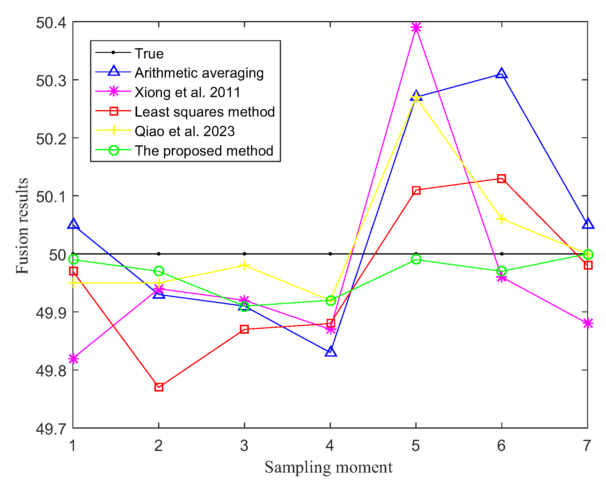
Since the accuracy information for each sensor is given in Table 7, the measurements need to be additionally fused using (11), (17), and (18). After a series of calculations, Figure 2 illustrates the measurement fusion results of the arithmetic averaging method, Xiong et al. [48], the least squares method, Qiao et al. [35], and the proposed method and the true value. From Figure 2, it can be observed that the proposed method is closer to the true value than the other methods, and the fluctuation in the fusion results of the other methods near the true value at different moments is larger with the proposed method, which is not conducive to the real-time fusion estimation of multiple sensors. It is further shown that the proposed method is not only adaptable to the measurements of different types of sensors, but also is adaptable to changes in the environment.
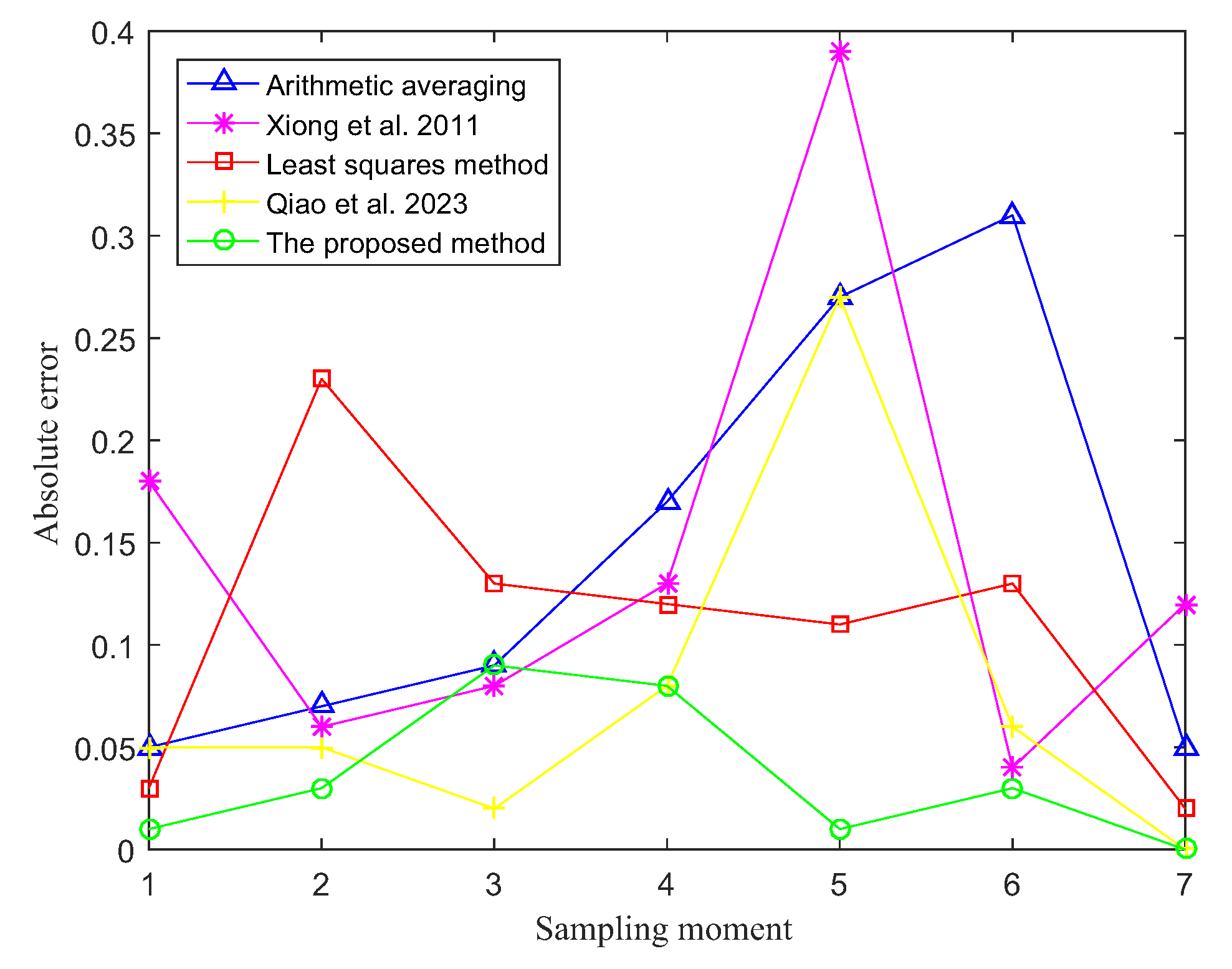
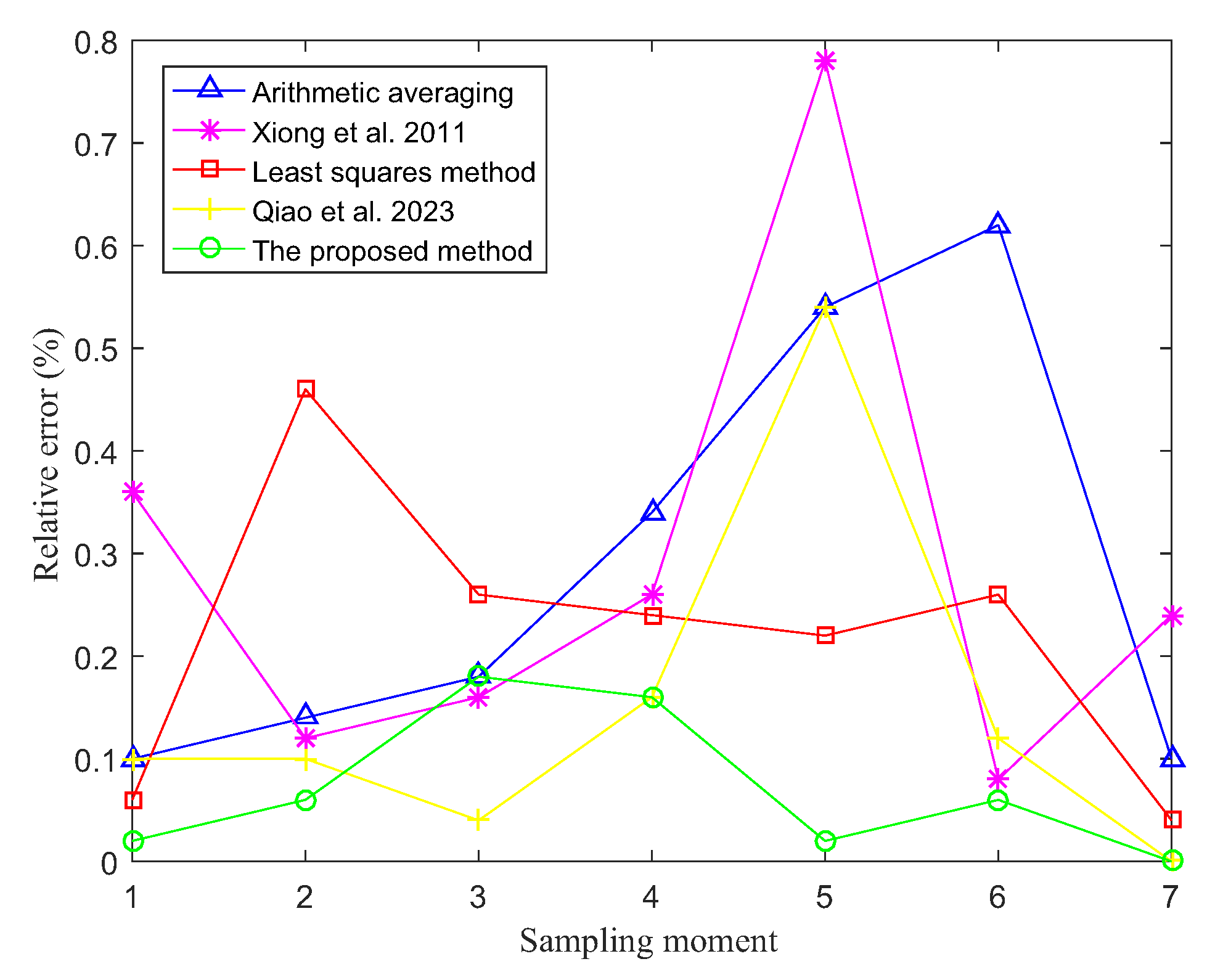
Figure 3 and Figure 4 exhibit the absolute and relative errors of measurement fusion for all methods. As shown in Figure 3 and Figure 4, the fusion result of the proposed method outperforms those of the other methods at any moment, except that it is poorer than the measurement fusion results of Qiao et al. [35] at the moment t 3 . At the moment t 5 , when the errors of the measurement fusion results of the other methods are relatively large, the proposed method still obtains a small measurement fusion error. Table 8 lists the average absolute and relative errors for multi-sensor multiple measurement fusion for all methods. From Table 8, we see that the average absolute and relative errors of the measurement fusion results of the proposed method are much smaller than those of the other methods, which indicates that the proposed method is more suitable for multi-sensor data fusion of control parameters compared to the other methods. The data collected by the multi-sensors at different moments also correspond to changes in the environmental conditions, which further demonstrates that the proposed method can still obtain higher quality fusion results under different environmental conditions.

5. Conclusions

In this paper, a fuzzy evidence theory multi-sensor data fusion method with belief divergence is developed to improve the fusion accuracy of the original existing evidence theory method. The method realizes the basic belief assignment in evidence theory by introducing the affiliation function and mutual support between sensor measurements. Then, the divergence measure is employed to measure the conflict between evidence pieces to minimize erroneous fusion results. In addition, the idea of evidence combination is utilized to achieve multi-sensor data fusion. Practical applications show that the proposed method is characterized by high fusion accuracy and robustness, which can avoid the limitation of a single sensor and reduce the effect of sensor uncertainty error and has theoretical significance and high engineering practical value. Converting the degree of data discrepancy into evidence more rationally to further improve the fusion performance of the proposed method will be the focus of future research.

Author Contributions

The work presented here was performed by collaboration among all the authors. S.Q. designed, analyzed, and wrote the paper; B.S. analyzed the data; Y.F. guided the full text; G.W. conceived the idea. All authors have read and agreed to the published version of the manuscript.

Funding

This research was supported by the National Key Research and Development Program of China(Grant number 2022YFB4301401), the National Natural Science Foundation of China (Grant number 61976033), the Pilot Base Construction and Pilot Verification Plan Program of Liaoning Province of China (Grant numbers 2022JH24/10200029), the Key Development Guidance Program of Liaoning Province of China(Grant numbers 2019JH8/10100100), and the China Postdoctoral Science Foundation (Grant number 2022M710569).

Institutional Review Board Statement

Not applicable.

Informed Consent Statement

Not applicable.

Data Availability Statement

Not applicable.

Conflicts of Interest

The authors declare no conflict of interest.

References

  1. Liu, D.; Zhang, J.; Jin, J.; Dai, Y.; Li, L. A new approach of obstacle fusion detection for unmanned surface vehicle using Dempster-Shafer evidence theory. Appl. Ocean. Res. 2022, 119, 103016. [Google Scholar] [CrossRef]
  2. Kim, J. Target following and close monitoring using an unmanned surface vehicle. IEEE Trans. Syst. Man Cybern. Syst. 2018, 50, 4233–4242. [Google Scholar] [CrossRef]
  3. Wu, Y.; Chu, X.; Deng, L.; Lei, J.; He, W.; Królczyk, G.; Li, Z. A new multi-sensor fusion approach for integrated ship motion perception in inland waterways. Measurement 2022, 200, 111630. [Google Scholar] [CrossRef]
  4. Liu, F.; Liu, Y.; Sun, X.; Sang, H. A new multi-sensor hierarchical data fusion algorithm based on unscented Kalman filter for the attitude observation of the wave glider. Appl. Ocean. Res. 2021, 109, 102562. [Google Scholar] [CrossRef]
  5. Mu, X.; He, B.; Wu, S.; Zhang, X.; Song, Y.; Yan, T. A practical INS/GPS/DVL/PS integrated navigation algorithm and its application on Autonomous Underwater Vehicle. Appl. Ocean. Res. 2021, 106, 102441. [Google Scholar] [CrossRef]
  6. Helgesen, Ø.K.; Vasstein, K.; Brekke, E.F.; Stahl, A. Heterogeneous multi-sensor tracking for an autonomous surface vehicle in a littoral environment. Ocean. Eng. 2022, 69, 111168. [Google Scholar] [CrossRef]
  7. Zhang, X.; Sheng, C.; Ouyang, W.; Zheng, L. Fault diagnosis of marine electric thruster bearing based on fusing multi-sensor deep learning models. Measurement 2023, 214, 112727. [Google Scholar] [CrossRef]
  8. Ye, J.; Roy, S.; Godjevac, M.; Baldi, S. A switching control perspective on the offshore construction scenario of heavy-lift vessels. IEEE Trans. Control. Syst. Technol. 2021, 29, 470–477. [Google Scholar] [CrossRef]
  9. Ye, J.; Roy, S.; Godjevac, M.; Baldi, S. Robustifying dynamic positioning of crane vessels for heavy lifting operation. IEEE/CAA J. Autom. Sin. 2021, 8, 753–765. [Google Scholar] [CrossRef]
  10. Fossen, T.I. An Adaptive Line-of-Sight (ALOS) Guidance Law for Path Following of Aircraft and Marine Craft. IEEE Trans. Control. Syst. Technol. 2023. [Google Scholar] [CrossRef]
  11. Xu, C.; Shi, Y.; Wan, J.; Duan, S. Uncertainty-Constrained Belief Propagation for Cooperative Target Tracking. IEEE Internet Things J. 2022, 9, 19414–19425. [Google Scholar] [CrossRef]
  12. Zhu, J.; Tang, Y.; Shao, X.; Xie, Y. Multisensor fusion using fuzzy inference system for a visual-IMU-wheel odometry. IEEE Trans. Instrum. Meas. 2021, 70, 1–16. [Google Scholar] [CrossRef]
  13. Li, C.; Wang, Z.; Song, W.; Zhao, S.; Wang, J.; Shan, J. Resilient Unscented Kalman Filtering Fusion With Dynamic Event-Triggered Scheme: Applications to Multiple Unmanned Aerial Vehicles. IEEE Trans. Control. Syst. Technol. 2022, 31, 370–381. [Google Scholar] [CrossRef]
  14. Li, D.; Shen, C.; Dai, X.; Zhu, X.; Luo, J.; Li, X.; Chen, H.; Liang, Z. Research on data fusion of adaptive weighted multi-source sensor. Comput. Mater. Contin. 2019, 61, 1217–1231. [Google Scholar] [CrossRef]
  15. Massignan, J.A.D.; London, J.B.A.; Bessani, M.; Maciel, C.D.; Fannucchi, R.Z.; Mir, A.V. Bayesian inference approach for information fusion in distribution system state estimation. IEEE Trans. Smart Grid 2022, 13, 526–540. [Google Scholar] [CrossRef]
  16. Ding, W.; Wang, J.; Rizos, C.; Kinlyside, D. Improving adaptive Kalman estimation in GPS/INS integration. J. Navig. 2007, 60, 517–529. [Google Scholar] [CrossRef] [Green Version]
  17. Lopes, N.V.; Couto, P.; Jurio, A.; Melo-Pinto, P. Hierarchical fuzzy logic based approach for object tracking. Knowl.-Based Syst. 2013, 54, 255–268. [Google Scholar]
  18. Fan, L.; Zhang, L. Multi-system fusion based on deep neural network and cloud edge computing and its application in intelligent manufacturing. Neural Comput. Appl. 2022, 34, 3411–3420. [Google Scholar] [CrossRef]
  19. Zhou, T.; Chen, M.; Zou, J. Reinforcement learning based data fusion method for multi-sensors. IEEE/CAA J. Autom. Sin. 2020, 7, 1489–1497. [Google Scholar] [CrossRef]
  20. Gao, B.; Hu, G.; Zhong, Y. Distributed state fusion using sparse-grid quadrature filter with application to INS/CNS/GNSS integration. IEEE Sens. J. 2021, 22, 3430–3441. [Google Scholar] [CrossRef]
  21. Li, A.; Zheng, B.; Li, L. Intelligent transportation application and analysis for multi-sensor information fusion of Internet of Things. IEEE Sens. J. 2021, 21, 25035–25042. [Google Scholar] [CrossRef]
  22. Cui, J.; Xie, P.; Wang, X.; Wang, J.; He, Q.; Jiang, G. M2FN: An end-to-end multi-task and multi-sensor fusion network for intelligent fault diagnosis. IEEE Trans. Instrum. Meas. 2022, 204, 112085. [Google Scholar] [CrossRef]
  23. Li, F.; Tang, Y.; Yue, X. Multi-sensor fusion Boolean Bayesian filtering for stochastic Boolean networks. IEEE Trans. Neural Netw. Learn. Syst. 2022. [Google Scholar] [CrossRef] [PubMed]
  24. Zhou, Z.; Xu, H.; Feng, H. A game theory-based fusion algorithm for autonomous navigation of smart ships. Measurement 2023, 216, 112897. [Google Scholar] [CrossRef]
  25. Zhu, C.; Xiao, F. A belief Hellinger distance for D–S evidence theory and its application in pattern recognition. Eng. Appl. Artif. Intell. 2021, 106, 104452. [Google Scholar] [CrossRef]
  26. Fan, W.; Xiao, F. A complex Jensen–Shannon divergence in complex evidence theory with its application in multi-source information fusion. Eng. Appl. Artif. Intell. 2022, 116, 105362. [Google Scholar] [CrossRef]
  27. Zhu, C.; Xiao, F. A belief Rényi divergence for multi-source information fusion and its application in pattern recognition. Appl. Intell. 2023, 53, 8941–8958. [Google Scholar] [CrossRef]
  28. Zeng, J.; Xiao, F. A fractal belief KL divergence for decision fusion. Eng. Appl. Artif. Intell. 2023, 121, 106027. [Google Scholar] [CrossRef]
  29. Wang, H.; Deng, X.; Jiang, W.; Geng, J. A new belief divergence measure for Dempster–Shafer theory based on belief and plausibility function and its application in multi-source data fusion. Eng. Appl. Artif. Intell. 2021, 97, 104030. [Google Scholar] [CrossRef]
  30. Deng, Z.; Wang, J. A new evidential similarity measurement based on Tanimoto measure and its application in multi-sensor data fusion. Eng. Appl. Artif. Intell. 2021, 104, 104380. [Google Scholar] [CrossRef]
  31. Ji, Z.; Tian, J.; Chen, H.; Liu, S. A new method for weighted fusion of evidence based on the unified trust distribution mechanism and the reward-punishment mechanism. Inf. Sci. 2023, 629, 798–815. [Google Scholar] [CrossRef]
  32. Zhao, K.; Sun, R.; Li, L.; Hou, M.; Yuan, G.; Sun, R. An improved evidence fusion algorithm in multi-sensor systems. Appl. Intell. 2021, 51, 7614–7624. [Google Scholar]
  33. Liu, B.; Deng, Y.; Cheong, K.H. An improved multisource data fusion method based on a novel divergence measure of belief function. Eng. Appl. Artif. Intell. 2022, 111, 104834. [Google Scholar]
  34. Shang, Q.; Li, H.; Deng, Y.; Cheong, K.H. Compound credibility for conflicting evidence combination: An autoencoder-K-means approach. IEEE Trans. Syst. Man Cybern. Syst. 2022, 52, 5602–5610. [Google Scholar] [CrossRef]
  35. Qiao, S.; Fan, Y.; Wang, G.; Zhang, H. Multi-Sensor Data Fusion Method Based on Improved Evidence Theory. J. Mar. Sci. Eng. 2023, 11, 1142. [Google Scholar] [CrossRef]
  36. Huang, Y.; Xiao, F. Higher order belief divergence with its application in pattern classification. Inf. Sci. 2023, 635, 1–24. [Google Scholar] [CrossRef]
  37. Ghosh, N.; Saha, S.; Paul, R. iDCR: Improved Dempster Combination Rule for multisensor fault diagnosis. Eng. Appl. Artif. Intell. 2021, 39, 104369. [Google Scholar] [CrossRef]
  38. Zhang, S.; Xiao, F. A TFN-based uncertainty modeling method in complex evidence theory for decision making. Inf. Sci. 2023, 619, 193–207. [Google Scholar] [CrossRef]
  39. Li, D.; Deng, Y.; Cheong, K.H. Multisource basic probability assignment fusion based on information quality. Int. J. Intell. Syst. 2021, 36, 1851–1875. [Google Scholar]
  40. Yaghoubi, V.; Cheng, L.; Van Paepegem, W.; Kersemans, M. CNN-DST: Ensemble deep learning based on Dempster–Shafer theory for vibration-based fault recognition. Struct. Health Monit. 2022, 21, 2063–2082. [Google Scholar] [CrossRef]
  41. Chen, L.; Deng, Y.; Cheong, K.H. Permutation Jensen–Shannon divergence for random permutation set. Eng. Appl. Artif. Intell. 2023, 119, 105701. [Google Scholar]
  42. Zhang, Y.; Hu, S.; Zhou, W. Multiple attribute group decision making using J-divergence and evidential reasoning theory under intuitionistic fuzzy environment. Neural Comput. Appl. 2020, 32, 6311–6326. [Google Scholar]
  43. Song, Y.; Deng, Y. A new method to measure the divergence in evidential sensor data fusion. Int. J. Distrib. Sens. Netw. 2019, 15, 1550147719841295. [Google Scholar]
  44. Xiao, F. Multi-sensor data fusion based on the belief divergence measure of evidences and the belief entropy. Inf. Fusion 2019, 46, 23–32. [Google Scholar]
  45. Pan, L.; Gao, X.; Deng, Y.; Cheong, K.H. Enhanced mass Jensen–Shannon divergence for information fusion. Expert Syst. Appl. 2022, 209, 118065. [Google Scholar]
  46. Van Erven, T.; Harremos, P. Rényi divergence and Kullback-Leibler divergence. IEEE Trans. Informat. Theory. 2014, 60, 3797–3820. [Google Scholar]
  47. Zhu, C.; Xiao, F.; Cao, Z. A generalized Rényi divergence for multi-source information fusion with its application in EEG data analysis. Inf. Sci. 2022, 605, 225–243. [Google Scholar]
  48. Xiong, Y.; Ping, Z. Data fusion algorithm inspired by evidence theory. J. Huazhong Univ. Sci. Technol. 2011, 39, 50–54. [Google Scholar]
  49. Xiong, Y.; Li, S.; Li, J.; Yang, Z. Novel data fusion algorithm for multi-sensor delay-control system. J. Proj. Rocket. Missiles Guid. 2012, 32, 171–174. [Google Scholar]
Figure 1. Flowchart of the conflicting measure and evidence synthesis.
Jmse 11 01596 g001
Figure 2. Fusion results for all methods [35,48].
Jmse 11 01596 g002
Figure 3. Absolute errors of measurement fusion for all methods [35,48].
Jmse 11 01596 g003
Figure 4. Relative errors of measurement fusion for all methods [35,48].
Jmse 11 01596 g004
Table 1. Thickness measurements of the sample.
NumberMeasurement ( μ m )NumberMeasurement ( μ m )
165.41566.45
265.76665.73
365.31765.81
465.35865.51
Table 2. Mass function for each evidence piece.
Basic Belief AssignmentMeasurements
Z 1 Z 2 Z 3 Z 4 Z 5 Z 6 Z 7 Z 8
m 1 ( Z 1 ) 0.16210.13780.12440.140100.14510.12170.1689
m 2 ( Z 2 ) 0.12810.17630.09760.110200.17830.15640.1531
m 3 ( Z 3 ) 0.15750.13610.13440.145800.14300.11940.1639
m 4 ( Z 4 ) 0.15900.13450.13200.148500.14180.11880.1653
m 5 ( Z 5 ) 0.12720.17370.09800.110100.17540.16480.1508
m 6 ( Z 6 ) 0.12990.17170.09900.111700.18040.15210.1552
m 7 ( Z 7 ) 0.12650.17480.09640.108800.17670.16540.1513
m 8 ( Z 8 ) 0.14970.14600.11460.129100.15370.12900.1779
Table 3. Fusion results of the proposed method with other methods.
MethodsFusion Results ( μ m )Absolute Error ( μ m )Relative Error (%)
Arithmetic averaging65.666250.096250.14678
Xiong et al. [48]65.560090.009910.01511
Qiao et al. [35]65.567850.002150.00328
Proposed method65.569990.000010.00002
Table 4. Multi-sensor measurements of device parameter.
Number12345
Measurements95.0398.7199.58101.79102.36
Table 5. The evidence mass function.
Basic Belief
Assignment
Measurements
Z 1 Z 2 Z 3 Z 4 Z 5
m 1 ( Z 1 ) 0.14820.14840.14440.13970
m 2 ( Z 2 ) 0.14740.14780.14540.14070
m 3 ( Z 3 ) 0.14690.14760.14680.14200
m 4 ( Z 4 ) 0.14660.14770.14650.14360
m 5 ( Z 5 ) 0.14660.14770.14670.14390
Table 6. Fusion results for the proposed and comparative methods.
MethodsFusion ResultsAbsolute ErrorRelative Error (%)
Arithmetic averaging99.4940.5060.506
Xiong et al. [48]99.9820.0180.018
Qiao et al. [35]100.0330.0330.033
Proposed method99.9980.0020.002
Table 7. Measurements and accuracy for each sensor.
Sensors σ i Sampling Moments
t 1 t 2 t 3 t 4 t 5 t 6 t 7
Z 1 0.4150.1449.2849.9549.9449.6349.9750.09
Z 2 0.5749.5649.9149.7549.9550.3749.6549.63
Z 3 0.5949.3550.0549.8249.7150.2750.1549.53
Z 4 0.7250.6650.0449.2050.3550.6949.8050.62
Z 5 0.8149.5650.5650.2149.8849.5351.4349.79
Z 6 0.8951.0349.7650.5449.1451.1550.8950.64
Table 8. Average errors for all methods.
MethodsAverage Absolute ErrorAverage Relative Error (%)
Arithmetic averaging0.14430.29
Xiong et al. [48]0.14290.29
Least squares method0.11000.22
Qiao et al. [35]0.07570.15
Proposed method0.03570.07
Disclaimer/Publisher’s Note: The statements, opinions and data contained in all publications are solely those of the individual author(s) and contributor(s) and not of MDPI and/or the editor(s). MDPI and/or the editor(s) disclaim responsibility for any injury to people or property resulting from any ideas, methods, instructions or products referred to in the content.