A Ship Tracking and Speed Extraction Framework in Hazy Weather Based on Deep Learning

Abstract

Obtaining ship navigation information from maritime videos can significantly improve maritime supervision efficiency and enable timely safety warnings. Ship detection and tracking are essential technologies for mining video information. However, current research focused on these advanced vision tasks in maritime supervision is not sufficiently comprehensive. Taking into account the application of ship detection and tracking technology, this study proposes a deep learning-based ship speed extraction framework under the haze environment. First, a lightweight convolutional neural network (CNN) is used to remove haze from images. Second, the YOLOv5 algorithm is used to detect ships in dehazed marine images, and a simple online and real-time tracking method with a Deep association metric (Deep SORT) is used to track ships. Then, the ship’s displacement in the images is calculated based on the ship’s trajectory. Finally, the speed of the ships is estimated by calculating the mapping relationship between the image space and real space. Experiments demonstrate that the method proposed in this study effectively reduces haze interference in maritime videos, thereby enhancing the image quality while extracting the ship’s speed. The mean squared error (MSE) for multiple scenes is 0.3 Kn on average. The stable extraction of ship speed from the video achieved in this study holds significant value in further ensuring the safety of ship navigation.

1. Introduction

Currently, the Automatic Identification System (AIS) serves as the primary platform for exchanging navigation information, including ship speed, between ships and between ships and the shore [1]. However, the rapid growth of the shipping industry has led to an increased number of ships, resulting in AIS signal interference in busy waters. Meanwhile, the system’s weak ability to combat data defects, system instability, and environmental interference often causes data delays or losses [2]. Additionally, some ships either lack AIS equipment or turn it off in monitored waters, thereby preventing the maritime supervision department from obtaining timely navigation information [3]. In this situation, both the supervisory authority and ships in the same waters are unable to obtain accurate and timely speed information of other ships, posing a hidden danger to navigation safety. Maritime videos, which provide rich information at a low cost, are widely used in maritime supervision. Techniques such as image processing, target detection, and target tracking are employed to identify obstacles at sea [4] and extract navigation information, such as ship trajectories, from maritime images [5]. These approaches have positive implications for enhancing maritime supervision efficiency and ensuring ship safety.

While several studies have been conducted on ship detection and tracking in maritime images [5,6,7], the related research has not sufficiently explored the application of ship detection and tracking technology, nor has it fully extracted the navigation information from maritime images. Zhao et al. [8] proposed a ship speed extraction framework based on UAV airborne video. In this study, the advantages of optical image data were fully utilized to realize the visual extraction of ship speed information. However, this study does not consider the influence of complex weather on the accuracy of ship speed extraction and lacks research on processing low-quality marine image data.

In this study, we propose a ship tracking and speed extraction framework based on deep learning under hazy weather conditions. Our approach utilizes cost-effective optical data while considering environmental impacts. We achieve ship speed information extraction from video data using ship tracking algorithms, as illustrated in Figure 1. The contributions of this study can be summarized as follows:

• To address the issue of the image becoming dark after haze removal, thereby obscuring the ship’s target features, we improved AOD-Net [9] at the pixel level. After haze removal, the mean peak signal-to-noise ratio (PSNR) of multiple maritime scenes reached 23.86, and the mean structural similarity index (SSIM) was 0.96, thus improving the quality of maritime images.
• We extract ship speed from the images based on the image mapping relationship. The average accuracy of ship speed extraction using this framework across multiple scenes is approximately 95%. Furthermore, the mean squared error (MSE) of the speed values extracted from the dehazed images is approximately 0.3 Kn lower than that extracted from the images before haze removal.
• Provides ideas for the application of advanced vision tasks such as haze removal from maritime haze images and ship tracking in maritime scenarios, improving the efficiency of maritime supervision.

2. Related Work

2.1. Image Haze Removal

Image processing for hazy weather is a significant research direction in the field of computer vision. Haze removal methods based on image enhancement primarily aim to enhance image contrast and highlight image details. These methods include the adaptive histogram equalization method [10], Retinex theory [11], etc. While these methods are simple, easy to implement, and widely applicable, they may lead to loss of details or over-enhancement. He et al. proposed a method of combining the dark channel prior with the atmospheric scattering model for haze removal [12]. The experimental principle of this method is simple and has a good effect on most natural scenes, but it is prone to local coloration or image brightness reduction after removing haze. In recent years, deep learning methods, such as convolutional neural networks (CNN), have been utilized for haze removal, and numerous deep networks have been developed for this purpose [9,13,14,15]; these haze removal networks have demonstrated improved results in haze removal experiments. However, most of these methods have been applied to land-based scenes, and there is a need for an improved haze removal network specifically tailored for maritime haze videos, considering the differences in sea surface scattering and other imaging characteristics compared to land-based haze. Therefore, this study enhances AOD-Net for maritime haze scenes to more efficiently remove haze from maritime haze images.

2.2. Target Tracking

Current methods of multi-target tracking generally employ the TBD (Tracking-by-Detection) strategy, which involves first detecting the target’s position in the image and then establishing associations between frames based on appearance consistency or positional similarity of the same target across frames. In recent years, with the advancement of algorithms such as deep learning, tracking accuracy has been enhanced by utilizing techniques such as neural networks to learn the appearance information of targets across different video frames for precise inter-frame associations [16,17,18]. However, the study by [19] demonstrates that when different tracking targets share similar appearance features, matching errors in target IDs can occur, making reliance solely on appearance features for inter-frame association unreliable.

Location similarity-based target tracking methods can overcome issues arising from the appearance similarity of tracked targets. Simple online and real-time tracking (SORT) [20] performs data association based on positional similarity and first uses a Kalman filter to predict the position of the track in the next frame and then calculates the Intersection over Union (IoU) between the detected and predicted frames. ByteTrack [21] matches the frames with IoU matching below the threshold twice to improve the tracking performance of the object when it is occluded. Inter-frame matching combining appearance consistency and location similarity can be sufficient to further improve tracking performance [22,23,24], and Deep SORT [25] uses an independent Re-ID model to extract appearance features from the detected frames to reduce ID matching errors. It is worth stating that the performance of the current multi-target tracking algorithm using the TBD strategy is closely related to the results of the detection model, and the performance of the tracking model can be guaranteed when the detection model reaches high accuracy [20]. In this paper, we adopt Deep SORT [25], a flexible and robust tracking model, after ensuring that yolov5 can detect ships with stable and high accuracy in maritime scenes.

2.3. Techniques for Obtaining Information on Ship Speed

Commonly used technologies for measuring ship speed include AIS [26], radar [27], lasers [28], and video-based speed measurements [29]. The emergence and advancement of the AIS system have provided robust technical support for acquiring ship navigation information [30]. However, as the number of ships at sea continues to increase, AIS signals are prone to interference. Other ships can only obtain ship navigation information [31] if the ship has AIS installed and turned on. Ship speed measurements using laser and radar technologies require specialized and costly equipment. In contrast, marine videos contain a wealth of ship navigation information, which can be easily visualized and processed in real-time. Additionally, visual sensors offer a wide monitoring range and are cost-effective [32], making them ideal for applications in complex marine environments with numerous ships and various influencing factors [33]. With the advancement of visual sensor technology, speed measurement methods based on videos hold promising prospects.

3. Materials and Methods

3.1. Remove Haze in Marine Haze Images Using CNN

The first part of the framework is a lightweight CNN, which is used to remove haze from hazy marine images. To improve the quality of marine images in complex scenes, marine haze images were used to train AOD-Net [9], which can achieve end-to-end dehazing in marine scenes. To avoid the darkening of the maritime images after haze removal by AOD-Net and to solve the problem of not highlighting the structural features of ships in the images after haze removal, Equation (1) was introduced to highlight further the structural features of ships in the images.

$$G\left(x\right)=mJ\left(x\right)+n$$

(1)

where, $J\left(x\right)$ is the image before image enhancement, $G\left(x\right)$ is the image after image enhancement, $m$ is the gain parameter, and $n$ is the bias parameter, which is used to adjust the contrast and brightness of the marine image to further eliminate the impact of background noise. In this study, the AOD-Net model trained by marine images and can improve the quality of images after haze removal is called e-AOD-Net. The e-AOD-Net uses a CNN to remove haze based on the atmospheric scattering model. The traditional atmospheric scattering model that generates hazy images is described as follows:

$$I\left(x\right)=J\left(x\right)t\left(x\right)+A\left(1-t\left(x\right)\right)$$

(2)

$$t\left(x\right)=e^{-\beta d\left(x\right)}$$

(3)

In the Equation (2), $I\left(x\right)$ is the hazy image, $J\left(x\right)$ is the clear image before image enhancement, and $t\left(x\right)$ is the medium transmission, describing the light without scattering and transmitted to the visual sensor, which can be expressed by the atmospheric scattering coefficient $\beta$ and the distance between the field and the visual sensor $d\left(x\right)$.

Equations (2) and (3) can be transformed into:

$$J\left(x\right)=K\left(x\right)I\left(x\right)-K\left(x\right)+b$$

(4)

$$K\left(x\right)=\frac{\frac{1}{t\left(x\right)}\left(I\left(x\right)-A\right)+\left(A-b\right)}{I\left(x\right)-1}$$

(5)

where, $b$ is the deviation value whose default value is 1. Meanwhile, Equation (4) integrates $\frac{1}{t\left(x\right)}$ and $A$ into $K\left(x\right)$. The e-AOD-Net builds an adaptive depth estimation model based on the physical model of atmospheric scattering and trains the network by minimizing the error between the pixel values of clear and hazy images.

As shown in Figure 2, $I\left(x\right)$ is entered into the network to estimate $K\left(x\right)$ and then input $K\left(x\right)$ into the dehazed image generation module as an adaptive parameter. The function of the $K\left(x\right)$ estimation module is to estimate the depth and haze concentration of hazy images. At the same time, Equation (1) is used to reduce the impact of noise on an image. Finally, clear images are synthesized by the multiplication and additional layers, and they can be output directly after haze removal to realize end-to-end haze removal of images.

3.2. Marine Shipping Target Detection Using the YOLOv5 Algorithm

The second part of the framework involves shipping detection. YOLO algorithms are representative of one-stage target detection algorithms, which regard target detection as a regression problem with a simple network flow. Among them, the YOLOv5 network is small, stable, and good in terms of network generalization ability [34], making it an ideal choice for real-time flexible target detection in the offshore environment. Because ships in maritime images are usually small and ship speed extraction has high requirements for the computational speed and flexibility of the detection algorithm, this framework adopts YOLOv5 as the target detection algorithm [35]. Meanwhile, the maritime dataset is used to train the YOLOv5 network to realize the fast and accurate positioning of small and medium-sized ships in maritime images and improve the accuracy of ship speed extraction. The main components of the YOLOv5 network are input, backbone, neck, and prediction, as shown in Figure 3.

Among them, mosaic enhancement is used at the input end of the YOLOv5 network to improve the detection accuracy of small ships. The adaptive anchor frame calculation and adaptive scaling for different data are performed to improve the calculation speed of the network. The neck network integrates the information of the upper and lower layers to fully extract the features of the ship. At the same time, the cross stage partial network (CSP-Net) is used to enhance the fusion of the target features of the network and improve the extraction efficiency of the ship’s features. In the prediction part of YOLOv5, the anchor frame of the grid is used for target detection on feature graphs of different scales. The complete intersection over union (CIoU) is used as the loss function of the boundary frame, which allows the algorithm to converge quickly and make the prediction frame more consistent with the real frame. Non-maximum suppression (NMS) is used by the neck network to enhance the detection accuracy of multiple ship targets and overlapping ship targets.

3.3. Ship Target Tracking with Deep SORT Algorithm

To obtain the pixel displacement of the ships in the images of continuous frames, the video with the detection frame information is taken as the input of the Deep SORT algorithm [8] in the third part of this framework. The algorithm first predicts the trajectory of the next frame using the Kalman filter. IOU matching and cascade matching are then performed between the predicted value and the detection frame information to track the trajectory of the target ship between the front and back frames of the video [36].

During the prediction process, $x_{k-1}=\left(u,v,r,h,\dot{x},\dot{y},\dot{z},\dot{h}\right)$ represents the motion state of the target in $k-1$ box, where $\left(u,v\right)$ is the central point coordinates of the target box, $r$ is the aspect ratio, and $h$ is the height of the detection box. In $x_{k-1}$, the last four variables are the derivatives of the first four variables, representing the transformation rate of the first four variables. When the standard filter is used to predict the motion state of the target, the last four values are constants. With $x_{k-1}=\left(u,v,r,h\right)$ as the prediction result, the motion state prediction of the Kalman algorithm can be expressed as:

$${\widehat{x}}_k=A{\widehat{x}}_{k-1}$$

(6)

where, ${\widehat{x}}_{k-1}$ is the motion state vector of frame $k-1$, and $A$ is the state transition matrix used to predict the motion state ${\widehat{x}}_k$ of frame $k$.

In the process of data association between continuous frames, Mahalanobis distance, and cosine distance are introduced to conduct the association of data between connected frames, and the thresholds between the observation box and prediction box are set, respectively. In the process of data association, when the Mahalanobis distance and cosine distance are both within the threshold range, the data association of two adjacent frames is considered successful. The comprehensive associated cost equation is as follows:

$$c_{i,j}=\lambda d^{\left(1\right)}\left(i,j\right)+\left(1-\lambda \right)d_{i,j}^{\left(2\right)}$$

(7)

where, $\lambda$ is a hyperparameter, and the influence of Mahalanobis distance and cosine distance on the association results can be controlled by controlling $\lambda$.

In order to enable the targets blocked for a long time to be continuously tracked, Deep SORT introduced cascade matching to give priority to the targets with more occurrences. Then, the intersection and union (IoU) between the boundary box and the prediction box by the Kalman filter is calculated and detected for the newly emerged targets and the prediction boxes that failed to match. The detection result is recognized if the match value is greater than the minimum IoU value. The equation for calculating IoU is as follows:

$$IoU=\frac{\left|area\left(A\right)\cap area\left(B\right)\right|}{\left|area\left(A\right)\cup area\left(B\right)\right|}$$

(8)

where, $A$ is the detection boundary box, and $B$ is the prediction boundary box of the candidate trajectory.

3.4. Space Mapping from 2D to 3D and Speed Extraction

In the fourth part, the mapping relation matrix between the ship’s displacement in the images and the actual displacement is obtained by 2D to 3D space mapping. The actual ship displacement is calculated according to the trajectory of the ship in the images obtained by the target tracking algorithm. The ship’s movement in a short time is regarded as the uniform motion. The average velocity equation is used to estimate the actual velocity of the ships based on the premise of knowing the time difference and actual displacement of the ship [37].

The process of 2D to 3D space mapping involves solving the mapping relationship between objects from the three-dimensional world and points on the two-dimensional image plane. The process involves four coordinate systems, and the representation methods of coordinate systems and points in coordinate systems are as follows:

(1)

World coordinate system. The coordinate system corresponding to the three-dimensional world describes the position of the target in the real world. The unit length of the coordinate axis is m. The points in the world coordinate system are represented by $\left(X_w,Y_w,Z_w\right)$.

(2)

Camera coordinate system. The origin is located in the optical center of the lens, and its x-axes and y-axes are parallel to both sides of the phase plane. The z-axis is perpendicular to the image plane and is the optical axis of the lens. The unit length of the coordinate axis is m. The points in the camera coordinate system are denoted as $\left(X_c,Y_c,Z_c\right)$.

(3)

Image coordinate system. The origin is the intersection of the optical axis of the camera and the imaging plane, that is, the midpoint of the imaging plane. The unit length of the coordinate axis is mm. The points in the image coordinate system are represented by $\left(x,y\right)$.

(4)

Pixel coordinate system: the origin is the top-left corner of the imaging plane in pixels. Points in the pixel coordinate system are represented as $\left(u,v\right)$.

The object is transformed from the world coordinate system to the camera coordinate system through translation and rotation, and the transformation equation between the camera coordinate system and the world coordinate system is:

$$\left[\begin{array}{c}{X}_c\\ Y_c\\ Z_c\\ 1\end{array}\right]=\left[\begin{array}{cc}R& t\\ \overrightarrow{0}& 1\end{array}\right]\left[\begin{array}{c}{X}_w\\ Y_w\\ Z_w\\ 1\end{array}\right]$$

(9)

where $R$ is a 3 × 3 rotation matrix and $t$ is a 3 × 1 translation vector.

The transformation of the camera coordinate system into the image coordinate system is based on the projection perspective. The connection between $P$ in space and the camera optical center $O$ is $OP$, and the intersection point $p$ between $OP$ and phase plane is the projection of point $P$ on the image as shown in Figure 4.

According to the projection perspective, the conversion equation of the camera coordinate system and the image coordinate system is:

$$Z_c\left[\begin{array}{c}x\\ y\\ z\\ 1\end{array}\right]=\left[\begin{array}{cccc}f& 0& 0& 0\\ 0& f& 0& 0\\ 0& 0& 1& 0\end{array}\right]\left[\begin{array}{c}{X}_c\\ Y_c\\ Z_c\\ 1\end{array}\right]$$

(10)

where $Z_c$ is the scale factor, and $f$ is the focal length. The pixel coordinate system can coincide with the image coordinate system after translation, as shown in Figure 5.

Then, the conversion equation of the image coordinate system and pixel coordinate system is:

$$\{\begin{array}{c}u=\frac{x}{d_x}+u_0\\ v=\frac{y}{d_y}+v_0\end{array}$$

(11)

Represented by the matrix:

$$\left[\begin{array}{c}u\\ v\\ 1\end{array}\right]=\left[\begin{array}{ccc}\frac{1}{d_x}& 0& u_0\\ 0& \frac{1}{d_y}& v_0\\ 0& 0& 1\end{array}\right]\left[\begin{array}{c}x\\ y\\ 1\end{array}\right]$$

(12)

where $d_x$ and $d_y$ are the scale factors of the two coordinate systems in the directions of the x-axis and y-axis, and $\left(u_0,v_0\right)$ is the coordinate of the origin of the pixel coordinate system.

As can be seen from Equations (9), (10), and (12), the conversion equation between the world coordinate system and the pixel coordinate system in which the image is located can be expressed as:

$$Z_c\left[\begin{array}{c}u\\ v\\ 1\end{array}\right]==\left[\begin{array}{cccc}\frac{f}{d_x}& 0& u_0& 0\\ 0& \frac{f}{d_y}& v_0& 0\\ 0& 0& 1& 0\end{array}\right]\left[\begin{array}{cc}R& t\\ \overrightarrow{0}& 1\end{array}\right]\left[\begin{array}{c}{X}_w\\ Y_w\\ Z_w\\ 1\end{array}\right]$$

(13)

If

$$\left[\begin{array}{cc}R& t\\ \overrightarrow{0}& 1\end{array}\right]=M$$

(14)

$$\left[\begin{array}{cccc}\frac{f}{d_x}& 0& u_0& 0\\ 0& \frac{f}{d_y}& v_0& 0\\ 0& 0& 1& 0\end{array}\right]=K$$

(15)

Then

$$Z_c\left[\begin{array}{c}u\\ v\\ 1\end{array}\right]=KM\left[\begin{array}{c}{X}_w\\ Y_w\\ Z_w\\ 1\end{array}\right]$$

(16)

In Equation (16), the element in $K$ is the configuration parameters of the camera, which is called the camera’s internal parameter matrix. The elements in $M$ are called the internal parameter matrix of the camera.

In this paper, the plane where the ship is located is set to the $X_w{O}_w{Y}_w$ plane of the world coordinate system, the direction perpendicular to $X_w{O}_w{Y}_w$ is the positive direction of the $Z_w$ axes, and the camera coordinate system is set to coincide with the world coordinate system. Under this assumption, the conversion equation of the pixel coordinate system and the world coordinate system can be simplified as:

$$Z_c\left[\begin{array}{c}u\\ v\\ 1\end{array}\right]=K\left[\begin{array}{c}{X}_w\\ Y_w\\ Z_w\\ 1\end{array}\right]$$

(17)

In this study, the ship’s movement in a very short time is regarded as uniform linear motion. Assuming that the ship displacement in the pixel coordinate system in the period $\Delta t$ at the moment $T$ can be expressed as $\left(\Delta u,\Delta v\right)$, the transformation relationship between the image displacement and actual displacement is as follows:

$$Z_c\left[\begin{array}{c}\Delta u\\ \Delta v\\ 1\end{array}\right]=K\left[\begin{array}{c}\Delta X_w\\ \Delta Y_w\\ \Delta Z_w\\ 1\end{array}\right]$$

(18)

Then the actual displacement of the ship in the time period $\Delta t$ is:

$$\Delta L=\sqrt{{\left(\Delta X_w\right)}^2+{\left(\Delta Y_w\right)}^2+{\left(\Delta Z_w\right)}^2}$$

(19)

According to the average velocity formula, the velocity of the ship at the moment $T$ can be expressed as:

$$v_T=\frac{\Delta L}{\Delta t}$$

(20)

4. Results

The main contents of Section 4 are the experimental details and results. It should be noted that all experiments were carried out on an Intel [email protected] GHz computer with a 6 g memory processor, and the experiments were completed in the Windows10 system using the Pytorch software library.

4.1. Experimental Data

In this study, contrast experiments were conducted on each module of the framework, and simulation experiments were conducted to verify the robustness of the framework in the process of extracting the shipping speed. The experimental data of hazy removal included three shore-based surveillance videos, which contained 5658 images, and three maritime videos with 8000 marine images. The resolution of the shore-based surveillance images is 640 × 386, and that of the self-built images is 1920 × 1080.

In the haze removal experiment of marine images, 5000 synthetic hazy marine images were selected as the training dataset to improve the generalization performance of AOD-Net on marine scenes, and 600 images were used as the non-repetitive test set. During the maritime target detection and tracking experiment, 8000 high-resolution images were divided into 6400 training datasets, 1000 validation datasets, and 600 test datasets to train the YOLOv5 algorithm. It should be noted that the training and test datasets do not overlap. At the same time, the Deep SORT algorithm was selected to combine with the YOLOv5 algorithm to conduct the multi-ship tracking experiment and the simulation experiment of ship speed extraction in marine scenarios. Shore-based scenes include scenes on cloudy days (scene 1 in Figure 6), scenes on sunny days [38] (scene 2 in Figure 6), and scenes with wave disturbance [38] (scene 3 in Figure 6). The self-built dataset includes the scene of many small target ships (scene 4 in Figure 6), the scene with normal light (scene 5 in Figure 6), and the scene with low light (scene 6 in Figure 6).

It should be noted that, when training the haze removal network, this paper [39] is referred to adding synthetic haze images to improve the generalization performance of the haze removal network in marine scenes. We synthesized image datasets with three different haze concentrations, and in this study, T represents the haze concentration. The images with three different haze concentrations are respectively represented as the images with $T=0.3$, the images with $T=0.5$, and the image data with $T=0.7$, among which the images with $T=0.3$ has the lowest haze concentration, as is shown in Figure 7.

4.2. Experimental Results and Analysis

4.2.1. Haze Removal of Marine Images

To verify the performance of the framework on haze removal, Retinex [40], Dark Channel Prior [12], Contrast Limited Adaptive Histogram Equalization (CLAHE) [41], AOD-Net [9], and e-AOD-Net adopted in the framework are used to conduct a comparative experiment on haze removal. The experimental results are shown in Figure 8.

The images generated by the above methods after haze removal are shown in Figure 8. Retinex and Dark Channel Prior usually lead to image distortion, and the color of the images after haze removal is seriously abnormal. CLAHE usually makes the color of images after haze removal too dark, and maritime ship features are not prominent. After haze removal by the AOD-Net network, there is still noise remaining in the images. These phenomena may occur because none of the above competing methods can fully extract the target structural features from ocean images. By contrast, e-AOD-Net can learn more structural features of images in marine scenes after generalization training and adaptive enhancement of marine images. The evaluation results of the dehazed images in multiple scenes using the PSNR and SSIM are presented in

Table 1. Evaluation results of dehazed images. (The best results are highlighted in red).

Method	Retinex		CLAHE		Dark Channel Prior		AOD-Net		e-AOD-Net
	PSNR 1	SSIM 2	PSNR	SSIM	PSNR	SSIM	PSNR	SSIM	PSNR	SSIM
Scene 1	10.86	0.70	9.80	0.67	9.72	0.72	22.81	0.94	23.71	0.95
Scene 2	10.12	0.68	9.06	0.65	9.01	0.67	20.50	0.95	21.86	0.94
Scene 3	10.10	0.65	9.51	0.63	9.09	0.65	20.06	0.95	23.84	0.95
Scene 4	10.73	0.55	9.76	0.52	9.48	0.53	20.59	0.92	21.99	0.95
Scene 5	11.42	0.40	10.46	0.38	11.13	0.39	22.15	0.92	23.69	0.96
Scene 6	11.79	0.50	10.17	0.43	10.82	0.48	19.68	0.94	23.87	0.96

¹ PSNR: The peak signal-to-noise ratio [42] is a widely used evaluation index for measuring image quality. ² SSIM: The structural similarity index measure [43] can objectively determine the structural similarity of images based on the human visual system.

.

As shown in Table 1, the e-AOD-Net adopted in this study has stable and good performance in multiple marine scenes, indicating that e-AOD-Net achieves better image enhancement performance. Images after haze removal can highlight more ship information, which is the basis of ship detection and tracking.

4.2.2. Multi-Ship Detection and Tracking Experiment after Images Enhancement

In this part, in order to verify the detection performance of the algorithm, SSD [44], Faster RCNN [45], and YOLO v4 [46] are compared with the YOLOv5 algorithm [47] adopted. The training comparison chart (Figure 9a), the verification comparison chart (Figure 9b), the frames per second (FPS) comparison chart (Figure 9c), the training index table (

Table 2. Train metrics.

	p	R	mAP_0.5	mAP_0.5:0.95
Faster RCNN	0.9446	0.9195	0.9297	0.8835
SSD	0.9154	0.8974	0.9065	0.8548
YOLO v4	0.979	0.9701	0.972	0.8903
YOLO v5	0.9929	0.973	0.989	0. 920

), the verification index table (

Table 3. Validation metrics.

	p	R	mAP_0.5	mAP_0.5:0.95
Faster RCNN	0.927	0.907	0.916	0.764
SSD	0.90.1	0.884	0.863	0.718
YOLO v4	0.973	0.982	0.995	0.845
YOLO v5	0.989	0.990	0.993	0.880

), the test index table (

Table 4. Test metrics.

	p	R	mAP_0.5	mAP_0.5:0.95
Faster RCNN	0.932	0.895	0.937	0.775
SSD	0.903	0.874	0.895	0.738
YOLO v4	0.983	0.979	0.991	0.80
YOLO v5	0.993	0.984	0.994	0.83

) are drawn respectively.

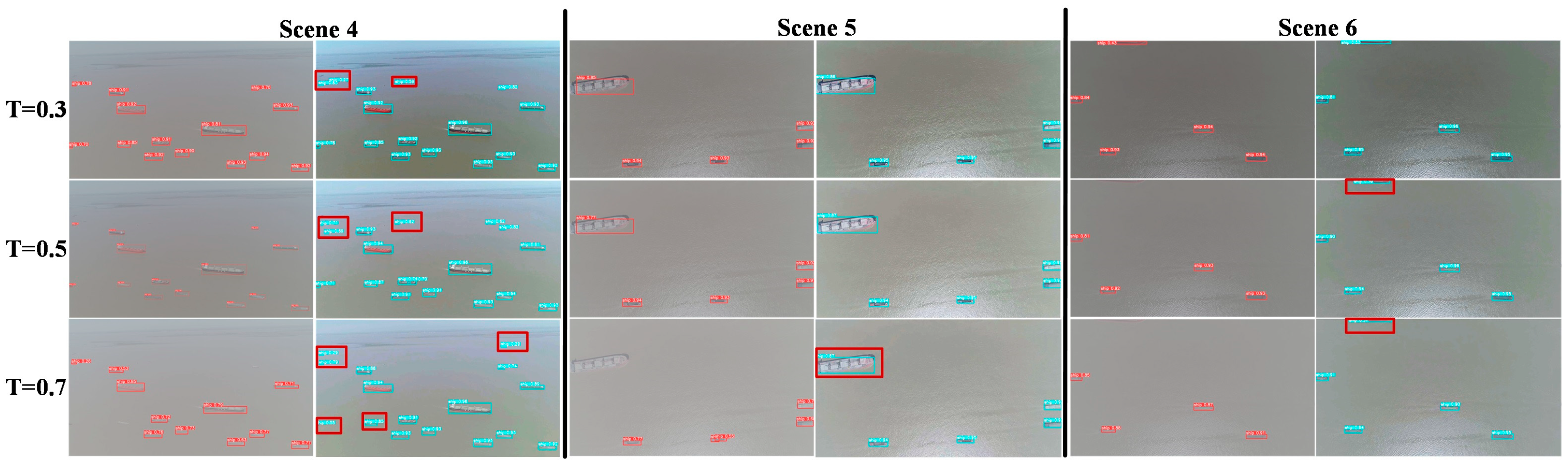
As can be seen from the comparison curve, under the same training conditions, the convergence speeds of the YOLOv4 and YOLOv5 algorithms are fast, and the YOLOv5 algorithm has a faster image-processing speed (in Figure 9c). The test and evaluation parameters show that the trained YOLOv5 algorithm also performs well in detecting accuracy in ocean scenes. To verify the performance of images after haze removal by e-AOD-Net in ship detection tasks, we adopted the stable YOLOv5 algorithm to detect ships in the synthesized hazy images and images after haze removal and compared the detection results. The detection results are presented in Figure 10.

Figure 10 shows that YOLOv5 has high-precision detection performance in multiple ocean scenarios. However, the degree of recovery of the images after haze removal is high, and the structural features of the ships are prominent, making it easy for the ship target in the image to be detected by the YOLOv5 algorithm, such as the small ships in the red boxes in scene 4. Haze noise in images reduces the accuracy of the target detection. In the case of high haze concentrations, some ships were not detected, such as those in the red boxes in scenes 5 and 6.

Considering the accuracy, detection speed, and detection stability of the algorithm in synthetic haze scenes, the YOLOv5 algorithm is ideal for ship detection in maritime scenarios. In the evaluation of the tracking algorithms, the YOLOv5 algorithm was used as the detector in scenarios 4, 5, and 6. In the three scenarios, multi-objective tracking evaluation parameters were introduced to evaluate the tracking performance of the SORT and Deep SORT algorithms for ships in ocean scenarios. The evaluation results are presented in

Table 5. Evaluation results of multi-ship tracking in scene 4.

Scene 4
Data Type	Tracker	Haze Concentration	IDF1 1 ↑	MOTA 2 ↑	MOTP 3 ↑	MT 4 ↑	ML 5 ↓	FP 6 ↓	FN 7 ↓	IDS 8 ↓
Hazy video	SORT	T = 0.3	97.6%	96.7%	85.4%	100.0%	0.0%	18	72	1
		T = 0.5	97.3%	95.1%	85.4%	100.0%	12.5%	20	114	2
		T = 0.7	89.3%	88.7%	84.2%	75.0%	12.5%	24	292	3
	Deep SORT	T = 0.3	98.5%	97.1%	85.2%	100.0%	0.0%	15	57	0
		T = 0.5	97.5%	95.6%	85.5%	100.0%	0.0%	20	92	1
		T = 0.7	96.8%	93.8%	84.7%	75.0%	12.5%	23	155	3
Dehazed video	SORT	T = 0.3	98.6%	97.3%	85.8%	100.0%	0.0%	14	58	0
		T = 0.5	97.7%	96.8%	86.0%	100.0%	0.0%	13	70	1
		T = 0.7	97.5%	95.9%	85.5%	100.0%	0.0%	17	89	2
	Deep SORT	T = 0.3	98.7%	97.5%	85.7%	100.0%	0.0%	3	44	0
		T = 0.5	98.7%	97.3%	86.9%	100.0%	0.0%	9	51	0
		T = 0.7	98.3%	96.7%	86.1%	100.0%	0.0%	14	71	0

¹ IDF1: The ratio of correctly identified detections over the average number of ground-truth and computed detections; ² MOTA (multi-object tracking accuracy): This measure combines three error sources: false positives, missed targets, and identity switches; ³ MOTP(Multiple Object Tracking Precision): The misalignment between the annotated and the predicted bounding boxes; ⁴ MT: The ratio of ground-truth trajectories that are covered by a track hypothesis for at least 80% of their respective life span; ⁵ ML: The ratio of ground-truth trajectories that are covered by a track hypothesis for at most 20% of their respective life span; ⁶ FP: The total number of false positives; ⁷ FN: The total number of false negatives (missed targets); ⁸ IDS: The total number of identity switches. (The meaning of the evaluation parameters in Table 6 and Table 7 is the same as described above.)

,

Table 6. Evaluation results of multi-ship tracking in scene 5.

Scene 5
Data Type	Tracker	Haze Concentration	IDF1 1 ↑	MOTA 2 ↑	MOTP 3 ↑	MT 4 ↑	ML 5 ↓	FP 6 ↓	FN 7 ↓	IDS 8 ↓
Hazy video	SORT	T = 0.3	92.7%	85.0%	80.4%	87.5%	0.0%	82	84	2
		T = 0.5	90.2%	81.2%	80.8%	87.5%	12.5%	106	248	1
		T = 0.7	88.4%	80.3%	77.6%	62.5%	25.0%	631	516	3
	Deep SORT	T = 0.3	98.0%	90.0%	81.5%	75.0%	0.0%	14	191	0
		T = 0.5	95.9%	94.0%	81.2%	87.5%	12.5%	39	263	1
		T = 0.7	95.3%	89.8%	80.7%	75.0%	12.5%	39	373	2
Dehazed video	SORT	T = 0.3	97.6%	93.2%	81.8%	87.5%	0.0%	54	149	0
		T = 0.5	95.1%	86.6%	81.4%	87.5%	12.5%	299	187	0
		T = 0.7	94.7%	88.1%	81.6%	87.5%	0.0%	456	201	0
	Deep SORT	T = 0.3	98.8%	95.7%	83.5%	87.5%	0.0%	16	50	0
		T = 0.5	98.0%	94.4%	81.6%	87.5%	0.0%	20	151	0
		T = 0.7	98.0%	94.0%	80.9%	87.5%	12.5%	23	177	0

and

Table 7. Evaluation results of multi-ship tracking in scene 6.

Scene 6
Data Type	Tracker	Haze Concentration	IDF1 1 ↑	MOTA 2 ↑	MOTP 3 ↑	MT 4 ↑	ML 5 ↓	FP 6 ↓	FN 7 ↓	IDS 8 ↓
Hazy video	SORT	T = 0.3	85.7%	78.9%	71.9%	85.7%	14.3%	183	3187	11
		T = 0.5	85.6%	75.0%	70.7%	85.7%	14.3%	226	4381	14
		T = 0.7	80.5%	70.2%	63.5%	71.4%	28.6%	318	4869	20
	Deep SORT	T = 0.3	86.2%	78.8%	74.4%	100.0%	0.0%	179	1356	9
		T = 0.5	85.4%	78.1%	72.4%	85.7%	28.6%	186	1267	12
		T = 0.7	82.7%	71.5%	65.6%	57.1%	28.6%	295	3741	18
Dehazed video	SORT	T = 0.3	86.8%	79.7%	75.5%	85.7%	14.3%	164	3171	12
		T = 0.5	85.7%	78.2%	71.9%	85.7%	14.3%	189	3469	14
		T = 0.7	83.2%	74.8%	68.5%	71.4%	28.6%	233	4715	14
	Deep SORT	T = 0.3	92.7%	82.1%	76.7%	100.0%	0.0%	120	1224	7
		T = 0.5	89.6%	79.9%	75.6%	85.7%	0.0%	163	1267	9
		T = 0.7	88.2%	79.3%	68.7%	85.7%	14.3%	204	1334	11

. In the tables, parameters with upward arrows indicate that the evaluated method performs better when the evaluated value is larger; those with downward arrows indicate that the evaluated method performs better when the evaluated value is smaller. And the optimal evaluation values when the hazy concentration is T = 0.3, T = 0.5, and T = 0.7 have been highlighted in red, yellow, and green, respectively in Table 5, Table 6 and Table 7.

As shown in Table 5, Table 6 and Table 7, the Deep SORT algorithm using YOLOv5 as a detector has higher MOTA and MOTP values as well as lower IDS and ML values in the above scenes. This indicates that Deep SORT can track ships stably while avoiding the number of ID transitions. It should be noted that in the same scenario, the evaluation results of tracking algorithms that use images after haze removal are usually the optimal values, indicating that images after haze removal can effectively improve the robustness of target tracking algorithms in maritime scenarios. It is worth noting that the YOLOv5 algorithm combined with the Deep SORT target tracking algorithm adopted in the framework can maintain high detection accuracy and stable tracking performance in multi-ship tracking, which is the basis for accurate ship speed extraction in this study.

4.2.3. Ship Speed Extraction

In this section, AIS data are considered as the ground truth of the ship speed values. The AIS data of Baosteel Wharf on 5 April 2021 is downloaded from the website http://www.shipxy.com. To make it easier to compare the ground truth of the ship speed values with the shipping speed extracted from marine images, the AIS data were linearly interpolated to match the video image frame by frame after extracting the speed data. To highlight the effect of this framework on hazy images and the performance of ship speed extraction, this section selects a ship in scenes 4, 5, and 6 for the speed extraction simulation experiment and compares the ground truth with the extracted speed of each ship in the scene with different haze concentrations. The extraction and comparison results for the ship speed are shown in Figure 11, Figure 12 and Figure 13. The mean speed of each ship and the MSE and MAE values compared to the ground truth of the speed are listed in

Table 8. Mean ship speeds.

	Haze Concentration	Mean Speed of Ship (Kn)
		Hazy Video	Dehazed Video	Ground Truth
Ship 1	T = 0.3	7.54	7.73	7.71
	T = 0.5	8.55	7.75
	T = 0.7	8.15	7.62
Ship 2	T = 0.3	7.59	7.50	7.50
	T = 0.5	7.71	7.54
	T = 0.7	7.50	7.58
Ship 3	T = 0.3	7.31	7.63	7.70
	T = 0.5	7.19	7.63
	T = 0.7	7.29	7.96

,

Table 9. MSE values of ship speed.

	Haze Concentration	MSE Values of Ship Speed (Kn)
		Hazy Video	Dehazed Video
Ship 1	T = 0.3	0.37	0.12
	T = 0.5	1.71	0.33
	T = 0.7	3.57	0.41
Ship 2	T = 0.3	0.32	0.13
	T = 0.5	0.43	0.13
	T = 0.7	0.57	0.18
Ship 3	T = 0.3	0.47	0.14
	T = 0.5	0.58	0.16
	T = 0.7	0.65	0.22

and

Table 10. MAE values of ship speed.

	Haze Concentration	MAE Values of Ship Speed (Kn)
		Hazy Video	Dehazed Video
Ship 1	T = 0.3	0.49	0.21
	T = 0.5	1.03	0.41
	T = 0.7	1.14	0.43
Ship 2	T = 0.3	0.44	0.23
	T = 0.5	0.50	0.26
	T = 0.7	0.54	0.30
Ship 3	T = 0.3	0.60	0.27
	T = 0.5	0.60	0.31
	T = 0.7	0.66	0.38

. In the Table 8, Table 9 and Table 10, the highlighted in yellow indicates the speed results and speed evaluation results extracted from the haze videos, the highlighted in green indicates the speed results and speed evaluation results extracted from the videos after haze removed, and the highlighted in red indicates the true value of speed extracted from the AIS data.

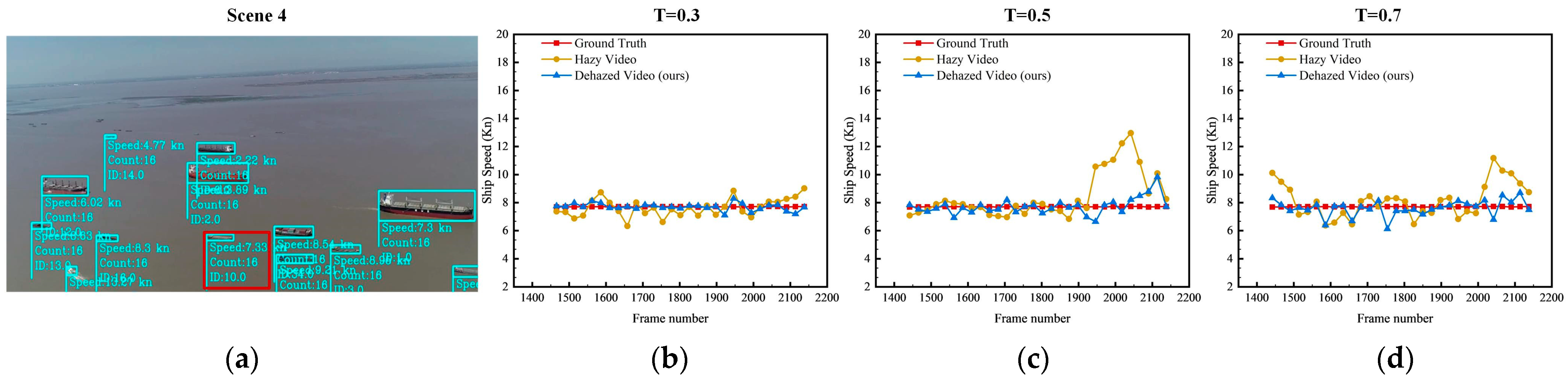
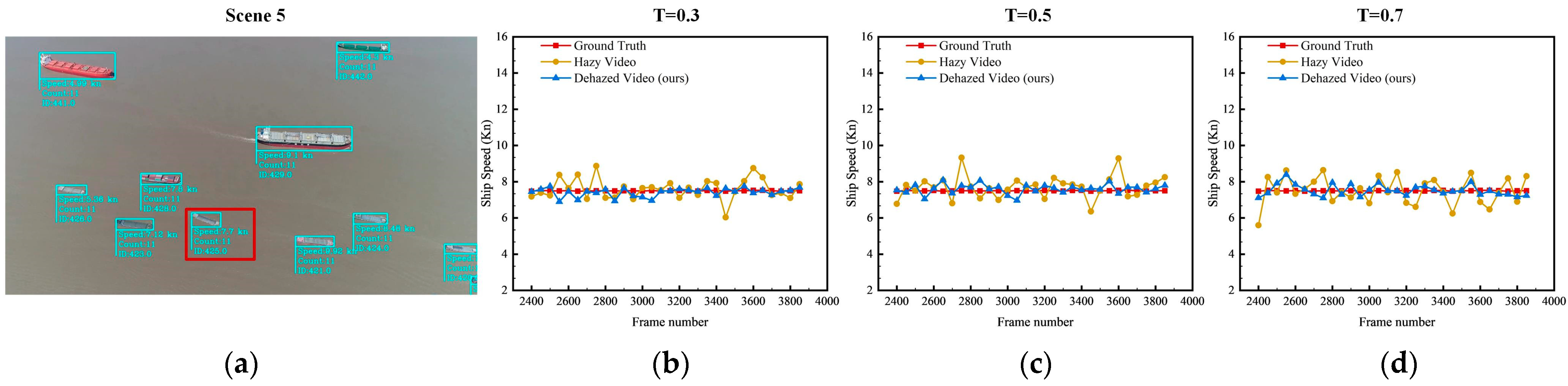
As shown in Figure 11, Figure 12 and Figure 13, the fold line representing the speed value of the ship extracted from the AIS data is set to red in the figure; the fold line graph representing the speed value of the ship extracted directly from the haze video is set to yellow, and the fold line representing the speed value of the ship extracted by our framework after removing the haze from the maritime haze image is set to blue. According to the extraction results and the mean ground truth of the ship speed, the speeds of the three ships were at 7.71 Kn, 7.50 Kn, and 7.70 Kn, respectively. For ship No. 1 in Figure 11, the accuracy of the speed extracted is easily affected by noise in the images owing to the small sizes of the ships. When T = 0.3, the MSE and MAE values of the speed are 0.37 Kn and 0.49 Kn due to the slight noise in the images. After haze removal, the fluctuation of the velocity image improved. At this time, the values of MSE are 0.12 Kn, the values of MAE are 0.21 Kn, and the ship’s average speed is improved from 7.54 Kn to 7.73 Kn, which is closer to the average speed of the ground truth of the ship speed.

When T = 0.5, due to the influence of haze noise in the images, the curve chart of ship velocity fluctuates wildly, especially in the late video period, and the MSE of ship velocity is 1.71 Kn, and MAE is 1.03 Kn. Although the extraction value of the velocity after haze removal still fluctuated, it was significantly improved compared with that before haze removal. After removing the haze, the MSE and MAE of the ship speed extracted from the image are 0.33 Kn and 0.41 Kn, and the average ship speed was 7.75 Kn.

When T = 0.7, the velocity fluctuation was more prominent. Currently, the MSE and MAE of ship velocity are 3.57 Kn and 1.14 Kn. After haze removal, the fluctuation of the velocity curve chart decreased. Both the MSE and MAE of the ship velocity decreased, and the mean value of the ship velocity was closer to the ground truth.

The same situation appeared in ship No. 2 in Figure 12. It can be seen from the truth line chart is approximately 7.5 Kn. According to the MSE and MAE of ship No. 2, the accuracy of the ship speed extracted can be improved by removing haze.

For ship No. 3 in scenario 6, the curve chart of ship speed fluctuates greatly because the image brightness is low, and the accuracy of the ship speed extracted is reduced after the haze noise is superimposed. The MSE of ship speed under different haze concentration environments was 0.47 Kn, 0.58 Kn, and 0.65 Kn, respectively. The MAE of speed is 0.60 Kn, 0.60 Kn, and 0.66 Kn. The MSE of speed extracted after removing haze is 0.14 Kn, 0.16 Kn, and 0.22 Kn. The MAE is 0.27 Kn, 0.31 Kn, and 0.38 Kn, respectively. After haze removal, the average ship speed extracted from the images was closer to the average value of the ground truth. It shows that the framework adopted in this paper can effectively enhance the quality of haze images in ocean scenes with low brightness and improve the accuracy of ship speed extracted from the images.

5. Conclusions

In this study, a framework for ship detection and ship speed extraction from maritime haze images using deep learning methods is proposed. First, a lightweight CNN was used to remove haze from hazy marine images. Second, YOLO v5 is used to accurately detect ships in marine images after haze removal. Moreover, the Deep-SORT target tracking algorithm is used to track ships. Finally, the ship motion pixels are calculated according to the trajectory information of the ship between adjacent image frames, and the ship speed is estimated and extracted based on the mapping relationship between the image space and the actual space.

Experimental results demonstrate that the proposed framework effectively enhances the clarity and contrast of marine haze images, as indicated by the mean peak signal-to-noise ratio (PSNR) and mean structural similarity index (SSIM) values of 23.86 and 0.96, respectively. The framework achieves high accuracy in extracting ship speed in multiple marine scenes, with an average accuracy above 95% and strong stability. The proposed speed extraction framework significantly improves the accuracy of ship speed extraction in hazy environments, with the mean squared error (MSE) values of ship speed extracted from the images after haze removal averaging 0.3 Kn lower than those from the images before haze removal.

In future studies, additional marine scenarios will be considered to further verify the practicality of this framework in real-world scenarios.

References

1. Qiao, D.; Liu, G.; Lv, T.; Li, W.; Zhang, J. Marine Vision-Based Situational Awareness Using Discriminative Deep Learning: A Survey. J. Mar. Sci. Eng. 2021, 9, 397. [Google Scholar] [CrossRef]
2. Chen, S.; Xiong, X.; Wen, Y.; Jian, J.; Huang, Y. State Compensation for Maritime Autonomous Surface Ships’ Remote Control. J. Mar. Sci. Eng. 2023, 11, 450. [Google Scholar] [CrossRef]
3. Chen, X.; Wang, Z.; Hua, Q.; Shang, W.L.; Luo, Q.; Yu, K. AI-Empowered Speed Extraction via Port-Like Videos for Vehicular Trajectory Analysis. IEEE Trans. Intell. Transp. Syst. 2022, 24, 4541–4552. [Google Scholar] [CrossRef]
4. Kang, B.S.; Jung, C.H. Detecting Maritime Obstacles Using Camera Images. J. Mar. Sci. Eng. 2022, 10, 1528. [Google Scholar] [CrossRef]
5. Chen, X.; Chen, W.; Yang, Y.; Li, C.; Han, B.; Yao, H. High-Fidelity Ship Imaging Trajectory Extraction via an Instance Segmentation Model. In Proceedings of the 2022 International Symposium on Sensing and Instrumentation in 5G and IoT Era (ISSI), Shanghai, China, 17–18 November 2022; Institute of Electrical and Electronics Engineers Inc.: Piscataway, NJ, USA, 2022; pp. 165–169. [Google Scholar]
6. Chen, X.; Xu, X.; Yang, Y.; Wu, H.; Tang, J.; Zhao, J. Augmented Ship Tracking under Occlusion Conditions from Maritime Surveillance Videos. IEEE Access 2020, 8, 42884–42897. [Google Scholar] [CrossRef]
7. Chen, Z.; Chen, D.; Zhang, Y.; Cheng, X.; Zhang, M.; Wu, C. Deep Learning for Autonomous Ship-Oriented Small Ship Detection. Saf. Sci. 2020, 130, 104812. [Google Scholar] [CrossRef]
8. Zhao, J.; Chen, Y.; Zhou, Z.; Zhao, J.; Wang, S.; Chen, X. Extracting Vessel Speed Based on Machine Learning and Drone Images during Ship Traffic Flow Prediction. J. Adv. Transp. 2022, 2022, 3048611. [Google Scholar] [CrossRef]
9. Li, B.; Peng, X.; Wang, Z.; Xu, J.; Feng, D. AOD-Net: All-in-One Dehazing Network. In Proceedings of the IEEE International Conference on Computer Vision, Venice, Italy, 22–29 October 2017; pp. 4780–4788. [Google Scholar] [CrossRef]
10. Ling, Z.; Liang, Y.; Wang, Y.; Shen, H.; Lu, X. Adaptive Extended Piecewise Histogram Equalisation for Dark Image Enhancement. IET Image Process 2015, 9, 1012–1019. [Google Scholar] [CrossRef]
11. Oishi, S.; Fukushima, N. Retinex-Based Relighting for Night Photography. Appl. Sci. 2023, 13, 1719. [Google Scholar] [CrossRef]
12. He, K.; Sun, J.; Tang, X. Single Image Haze Removal Using Dark Channel Prior. IEEE Trans. Pattern Anal. Mach. Intell. 2011, 33, 2341–2353. [Google Scholar] [CrossRef]
13. Yeh, C.H.; Huang, C.H.; Kang, L.W. Multi-Scale Deep Residual Learning-Based Single Image Haze Removal via Image Decomposition. IEEE Trans. Image Process. 2020, 29, 3153–3167. [Google Scholar] [CrossRef]
14. He, L.; Bai, J.; Ru, L. Haze Removal Using Aggregated Resolution Convolution Network. IEEE Access 2019, 7, 123698–123709. [Google Scholar] [CrossRef]
15. Qin, M.; Xie, F.; Li, W.; Shi, Z.; Zhang, H. Dehazing for Multispectral Remote Sensing Images Based on a Convolutional Neural Network with the Residual Architecture. IEEE J. Sel. Top. Appl. Earth Obs. Remote Sens. 2018, 11, 1645–1655. [Google Scholar] [CrossRef]
16. Bergmann, P.; Meinhardt, T.; Leal-Taixe, L. Tracking without Bells and Whistles. In Proceedings of the 2019 IEEE/CVF International Conference on Computer Vision (ICCV), Seoul, Republic of Korea, 27 October–2 November 2019. [Google Scholar] [CrossRef] [Green Version]
17. Chu, P.; Wang, J.; You, Q.; Ling, H.; Liu, Z. TransMOT: Spatial-Temporal Graph Transformer for Multiple Object Tracking. arXiv arXiv:2104.00194, 2021.
18. Brasó, G.; Leal-Taixé, L. Learning a Neural Solver for Multiple Object Tracking. arXiv 2019, arXiv:1912.07515. [Google Scholar]
19. Yang, F.; Odashima, S.; Masui, S.; Jiang, S. Hard to Track Objects with Irregular Motions and Similar Appearances? Make It Easier by Buffering the Matching Space. arXiv 2022, arXiv:2211.14317. [Google Scholar]
20. Bewley, A.; Ge, Z.; Ott, L.; Ramos, F.; Upcroft, B. Simple Online and Realtime Tracking. In Proceedings of the 2016 IEEE International Conference on Image Processing (ICIP), Phoenix, AZ, USA, 25–28 September 2016; pp. 3464–3468. [Google Scholar] [CrossRef] [Green Version]
21. Zhang, Y.; Sun, P.; Jiang, Y.; Yu, D.; Weng, F.; Yuan, Z.; Luo, P.; Liu, W.; Wang, X. ByteTrack: Multi-Object Tracking by Associating Every Detection Box. arXiv 2021, arXiv:2110.06864. [Google Scholar]
22. Pang, J.; Qiu, L.; Li, X.; Chen, H.; Li, Q.; Darrell, T.; Yu, F. Quasi-Dense Similarity Learning for Multiple Object Tracking. In Proceedings of the IEEE/CVF Conference on Computer Vision and Pattern Recognition (CVPR), Online, 13–19 June 2020. [Google Scholar]
23. Wang, Z.; Zheng, L.; Liu, Y.; Li, Y.; Wang, S. Towards Real-Time Multi-Object Tracking. arXiv 2019, arXiv:1909.12605. [Google Scholar]
24. Zhang, Y.; Wang, C.; Wang, X.; Liu, W.; Zeng, W. VoxelTrack: Multi-Person 3D Human Pose Estimation and Tracking in the Wild. arXiv 2021, arXiv:2108.02452. [Google Scholar] [CrossRef]
25. Wojke, N.; Bewley, A.; Paulus, D. Simple Online and Realtime Tracking with a Deep Association Metric. In Proceedings of the 2017 IEEE International Conference on Image Processing (ICIP), Beijing, China, 17–20 September 2017; pp. 3645–3649. [Google Scholar]
26. Abebe, M.; Shin, Y.; Noh, Y.; Lee, S.; Lee, I. Machine Learning Approaches for Ship Speed Prediction towards Energy Efficient Shipping. Appl. Sci. 2020, 10, 2325. [Google Scholar] [CrossRef] [Green Version]
27. Electronics, A.; Electric, M.; Kamakura, C.; Kamimachiya, W.; Kanagawa, K. Radar Speed Monitoring System. In Proceedings of the VNIS’94-1994 Vehicle Navigation and Information Systems Conference, Yokohama, Japan, 31 August–2 September 1994; pp. 89–93. [Google Scholar] [CrossRef]
28. Musayev, E. Laser-Based Large Detection Area Speed Measurement Methods and Systems. Opt. Lasers Eng. 2007, 45, 1049–1054. [Google Scholar] [CrossRef]
29. Li, J.; Chen, S.; Zhang, F.; Li, E.; Yang, T.; Lu, Z. An Adaptive Framework for Multi-Vehicle Ground Speed Estimation in Airborne Videos. Remote Sens. 2019, 11, 1241. [Google Scholar] [CrossRef] [Green Version]
30. Chen, X.; Liu, S.; Liu, R.W.; Wu, H.; Han, B.; Zhao, J. Quantifying Arctic Oil Spilling Event Risk by Integrating an Analytic Network Process and a Fuzzy Comprehensive Evaluation Model. Ocean Coast. Manag. 2022, 228, 106326. [Google Scholar] [CrossRef]
31. Wolsing, K.; Roepert, L.; Bauer, J.; Wehrle, K. Anomaly Detection in Maritime AIS Tracks: A Review of Recent Approaches. J. Mar. Sci. Eng. 2022, 10, 112. [Google Scholar] [CrossRef]
32. Chen, X.; Xu, X.; Yang, Y.; Huang, Y.; Chen, J.; Yan, Y. Visual Ship Tracking via a Hybrid Kernelized Correlation Filter and Anomaly Cleansing Framework. Appl. Ocean Res. 2021, 106, 102455. [Google Scholar] [CrossRef]
33. Ren, Y.; Yang, J.; Zhang, Q.; Guo, Z. Ship Recognition Based on Hu Invariant Moments and Convolutional Neural Network for Video Surveillance. Multimed. Tools Appl. 2021, 80, 1343–1373. [Google Scholar] [CrossRef]
34. Suliva, R.S.S.; Valencia, C.A.A.; Villaverde, J.F. Classification and Counting of Ships Using YOLOv5 Algorithm. In Proceedings of the 2022 6th International Conference on Communication and Information Systems (ICCIS), Chongqing, China, 14–16 October 2022; pp. 153–158. [Google Scholar] [CrossRef]
35. Jia, Z.; Su, X.; Ma, G.; Dai, T.; Sun, J. Crack Identification for Marine Engineering Equipment Based on Improved SSD and YOLOv5. Ocean Eng. 2023, 268, 113534. [Google Scholar] [CrossRef]
36. Jie, Y.; Leonidas, L.; Mumtaz, F.; Ali, M. Ship Detection and Tracking in Inland Waterways Using Improved Yolov3 and Deep Sort. Symmetry 2021, 13, 308. [Google Scholar] [CrossRef]
37. Zhang, Z. Flexible Camera Calibration by Viewing a Plane from Unknown Orientations. In Proceedings of the Seventh IEEE International Conference on Computer Vision, Kerkyra, Greece, 20–27 September 1999; Volume 1, pp. 666–673. [Google Scholar] [CrossRef]
38. Prasad, D.K.; Rajan, D.; Rachmawati, L.; Rajabally, E.; Quek, C. Video Processing from Electro-Optical Sensors for Object Detection and Tracking in a Maritime Environment: A Survey. IEEE Trans. Intell. Transp. Syst. 2017, 18, 1993–2016. [Google Scholar] [CrossRef] [Green Version]
39. Liu, R.W.; Yuan, W.; Chen, X.; Lu, Y. An Enhanced CNN-Enabled Learning Method for Promoting Ship Detection in Maritime Surveillance System. Ocean Eng. 2021, 235, 109435. [Google Scholar] [CrossRef]
40. Wei, C.; Wang, W.; Yang, W.; Liu, J. Deep Retinex Decomposition for Low-Light Enhancement. arXiv 2019, arXiv:1808.04560. [Google Scholar]
41. Yadav, G.; Maheshwari, S.; Agarwal, A. Contrast Limited Adaptive Histogram Equalization Based Enhancement for Real Time Video System. In Proceedings of the 2014 International Conference on Advances in Computing, Communications and Informatics (ICACCI), Delhi, India, 24–27 September 2014; pp. 2392–2397. [Google Scholar] [CrossRef]
42. Wang, Z.; Bovik, A.C. Mean Squared Error: Love It or Leave It? A New Look at Signal Fidelity Measures. IEEE Signal Process. Mag. 2009, 26, 98–117. [Google Scholar] [CrossRef]
43. Wang, Z.; Bovik, A.C.; Sheikh, H.R.; Simoncelli, E.P. Image Quality Assessment: From Error Visibility to Structural Similarity. IEEE Trans. Image Process. 2004, 13, 600–612. [Google Scholar] [CrossRef] [Green Version]
44. Liu, W.; Anguelov, D.; Erhan, D.; Szegedy, C.; Reed, S.; Fu, C.Y.; Berg, A.C. SSD: Single Shot Multibox Detector; Lecture Notes in Computer Science (Including Subseries Lecture Notes in Artificial Intelligence and Lecture Notes in Bioinformatics); Springer: Cham, Switzerland, 2016; 9905 LNCS; pp. 21–37. [Google Scholar]
45. Ren, S.; He, K.; Girshick, R.; Sun, J. Faster R-CNN: Towards Real-Time Object Detection with Region Proposal Networks. IEEE Trans. Pattern Anal. Mach. Intell. 2017, 39, 1137–1149. [Google Scholar] [CrossRef] [Green Version]
46. Bochkovskiy, A.; Wang, C.-Y.; Liao, H.-Y.M. YOLOv4: Optimal Speed and Accuracy of Object Detection 2020. arXiv 2020, arXiv:2004.10934. [Google Scholar]
47. Kim, J.H.; Kim, N.; Park, Y.W.; Won, C.S. Object Detection and Classification Based on YOLO-V5 with Improved Maritime Dataset. J. Mar. Sci. Eng. 2022, 10, 377. [Google Scholar] [CrossRef]
Figure 1. Frame diagram of the method.
Jmse 11 01353 g001
Figure 2. Haze removal network.
Jmse 11 01353 g002
Figure 3. The network structure of YOLOv5.
Jmse 11 01353 g003
Figure 4. Projection perspective between the camera coordinate system and the image coordinate system.
Jmse 11 01353 g004
Figure 5. Translation relationship between the image coordinate system and the pixel coordinate system.
Jmse 11 01353 g005
Figure 6. Experimental scenes.
Jmse 11 01353 g006
Figure 7. Synthetic haze images.
Jmse 11 01353 g007
Figure 8. Comparative experiments of haze removal. (a) Retinex (b) Dark Channel Prior (c) CLAHE (d) AOD-Net (e) e-AOD-Net.
Jmse 11 01353 g008
Figure 9. Comparison of detection methods. (a) Training carve; (b) Validation carve; (c) FPS of multiple detection algorithms.
Jmse 11 01353 g009
Figure 10. Comparison of detection effects of YOLOv5 on images before and after haze removal (Detection details are highlighted with red boxes).
Jmse 11 01353 g010
Figure 11. Speed extraction results for ship 1 in scene 4. (a) Scene image; (b) Comparison of speed measurements (T = 0.3); (c) Comparison of speed measurements (T = 0.5); (d) Comparison of speed measurements (T = 0.7).
Jmse 11 01353 g011
Figure 12. Speed extraction results for ship 2 in scene 5. (a) Scene image; (b) Comparison of speed measurements (T = 0.3); (c) Comparison of speed measurements (T = 0.5); (d) Comparison of speed measurements (T = 0.7).
Jmse 11 01353 g012
Figure 13. Speed extraction results for ship 3 in scene 6. (a) Scene image; (b) Comparison of speed measurements (T = 0.3); (c) Comparison of speed measurements (T = 0.5); (d) Comparison of speed measurements (T = 0.7).
Jmse 11 01353 g013