Research on Multi-Port Ship Traffic Prediction Method Based on Spatiotemporal Graph Neural Networks

Abstract

The intelligent maritime transportation system has emerged as a pivotal component in port management, owing to the rapid advancements in artificial intelligence and big data technology. Its essence lies in the application of digital modeling techniques, which leverage extensive ship data to facilitate efficient operations. In this regard, effective modeling and accurate prediction of the fluctuation patterns of ship traffic in multiple port regions will provide data support for trade analysis, port construction planning, and traffic safety management. In order to better express the potential interdependencies between ports, inspired by graph neural networks, this paper proposes a data-driven approach to construct a multi-port network and designs a spatiotemporal graph neural network model. The model incorporates graph attention networks and a dilated causal convolutional architecture to capture the temporal and spatial dimensions of traffic variation patterns. It also employs a gated-mechanism-based spatiotemporal bi-dimensional feature fusion strategy to handle the potential unequal relationships between the two dimensions of features. Compared to existing methods for port traffic prediction, this model fully considers the network characteristics of the overall port and fills the research gap in multi-port scenarios. In the experiments, real port ship traffic datasets were constructed using data from the Automatic Identification System (AIS) and port geographical information data for model validation. The results demonstrate that the model exhibits outstanding robustness and performs well in predicting traffic in multiple sub-regional port clusters.

1. Introduction

Maritime transportation, characterized by its substantial carrying capacity, cost-effectiveness, and remarkable adaptability to diverse environmental conditions, plays a significant role in international trade as an important mode of transportation. The accurate prediction of ship traffic flow holds immense significance, as it offers invaluable data support for the advancement of the national maritime industry and the strategic planning of international trade initiatives. Furthermore, it plays a crucial role in facilitating port layout planning, thereby addressing the prevalent challenge of aligning the port capacity with the escalating number of vessels arising from the rapid growth of the maritime industry. Additionally, this predictive capability contributes to the reduction of traffic congestion and the mitigation of accidents within maritime areas, consequently enhancing the overall efficiency of port infrastructure utilization [1].

This paper primarily concentrates on the prediction of maritime traffic flow in multi-port scenarios. Traffic flow prediction entails a typical task of time series forecasting, wherein the objective is to capture inherent patterns within traffic flow and speed data, characterized by their temporal sequences. By effectively discerning such patterns, it becomes feasible to infer future traffic flow states [2]. The primary challenge in time series prediction lies in accurately extracting a consistent temporal pattern. In practice, numerous factors, including environmental fluctuations, seasonal variations, and unforeseen accidents, can disrupt these theoretically stable patterns, thereby adding a considerable level of complexity to time series prediction problems. Consequently, time series prediction methods necessitate the incorporation of diverse influencing factors [3].

In the past, linear methods such as Autoregressive Integrated Moving Average (ARIMA) models and historical average analysis were limited in handling complex external factors. Scholars have attempted to use nonlinear machine learning methods such as backpropagation networks [4] and support vector machines [5] to uncover hidden patterns in time series data. However, these methods often suffer from slow convergence and algorithmic incompleteness, resulting in unsatisfactory solutions to time series prediction problems.

Consequently, researchers have turned to the application of deep learning techniques as a means to tackle practical time series prediction challenges. Deep neural networks exhibit the inherent capability to capture and model nonlinear relationships. By leveraging the stacking of multiple layers, these models can effectively capture a multitude of hidden factors and intricate variables within the data. Recurrent neural networks (RNN) [6], long short-term memory (LSTM) [7], and subsequent models such as gated recurrent units (GRU) [8], WaveNet [9], and Transformer [10,11], have demonstrated outstanding performance in the field of time series prediction.

With the rapid development of graph neural networks in recent years, spatial-convolution-based graph neural network models led by graph convolutional networks (GCN) [12] and graph attention networks (GAN) [13] have gained significant attention. In graph neural networks, a graph is composed of a set of vertices (nodes) that are interconnected by a set of edges. By performing convolutions on graphs with arbitrary structures, graph neural networks can learn rich spatial features. In recent years, they have been successfully applied in various domains, such as trajectory prediction [14,15] and traffic flow prediction [16].

In traffic flow prediction methods, conventional approaches often consider traffic intersections or sensors as entities, represented as individual nodes. Simultaneously, the road network, which accommodates these traffic entities, serves as the edges that symbolize the relationships between these nodes. Graph neural-network-based traffic flow prediction methods aggregate traffic flow information from neighboring nodes within a local spatial range, thereby predicting the potential information of nodes in the traffic subnetwork.

Nevertheless, relying solely on spatial information to predict traffic flow states is not rigorous and can lead to a significant loss of temporal information. To address this limitation, researchers have extended their efforts by incorporating temporal prediction learning methods into graph neural networks [17]. By leveraging techniques such as gate units and recurrent neural networks (RNN), they have introduced “spatiotemporal graph” models, which effectively capture both the spatial and temporal features of traffic flow prediction [18,19]. These spatiotemporal graph models take into account both temporal patterns and the spatial correlation structure of traffic entities. They can effectively capture the underlying meanings and interactions of nodes and edges within complex systems, resulting in superior prediction performance in traffic flow prediction.

In recent years, numerous excellent spatiotemporal graph models have been proposed and applied in the field of urban traffic prediction. Representative works include Multivariate Time Series Forecasting with Graph Neural Networks (MTGNN) [20], Diffusion Convolutional Recurrent Neural Networks (DCRNN) [21], Spatiotemporal Graph Convolutional Networks (STGCN) [18], and others.

However, the application traffic flow prediction methods in the maritime domain still faces two major challenges. Firstly, there is a scarcity of public datasets that can be directly used for analysis. The process of constructing maritime traffic flow datasets is arduous and complex. Secondly, the maritime traffic flow prediction scenarios do not possess the same traffic network structures as urban settings, rendering it difficult to directly apply spatiotemporal graph methods developed for urban traffic flow prediction [22]. Existing port flow prediction methods typically focus on single-port scenarios and do not fully consider the characteristics of port networks. They fail to consider the patterns of flow changes from the perspective of the overall port distribution structure, resulting in a relative scarcity of research in multi-port scenarios [23].

The scarcity of maritime traffic datasets stems primarily from the extensive geographical distribution, intricate structural arrangements, and challenges in regulating the maritime networks comprising ports across diverse countries. The widespread adoption of the Automatic Identification System (AIS) has significantly addressed the data gap in the maritime domain. The AIS is an onboard broadcast response system that has been gradually deployed on international vessels since 2002 and now has achieved widespread coverage through satellite networks. Vessels equipped with AIS devices regularly transmit navigational status data such as position points, speed, heading, and identity to ground-based stations and satellite receivers [24]. This enables data exchange between vessels and assists in navigation.

Despite the development of AIS, there are significant challenges related to the noise contamination in the raw AIS data, which limits their application in maritime traffic systems [25]. In this study, we address this issue by combining AIS data with spatial information from various ports worldwide and employing various big data processing techniques, similar to [26]. Through these approaches, we are able to effectively filter out noisy AIS data to the maximum extent possible and reconstruct realistic maritime traffic flow scenarios. As a result, we have constructed a multi-port flow dataset that can assist in conducting in-depth research on ship traffic flow prediction and validating the effectiveness of models under fair conditions.

The second challenge is that most existing research focuses on specific and single-port traffic flow scenarios, while studies on wide-scale, networked, and multi-port ship traffic flow prediction are relatively scarce. For example, ref. [27] combines Kalman filtering with regression analysis to improve short-term ship traffic flow prediction performance. Ref. [28] proposes a multi-variable extended CNN model based on convolutional methods, which specifically considers the impact of extreme weather events on ship traffic flow changes. However, the experimental settings in [28] involve geographically close ship traffic statistical areas, failing to consider the complex correlation structures among multiple regions. Ref. [29] uses AIS data to analyze the hourly ship traffic volume in a specific area near Ningbo and achieves ship traffic flow prediction for multiple time periods using an improved GRU-based time series prediction model. Nevertheless, it is also limited to the task of predicting traffic flow in a single maritime area.

This article tackles the challenge of ship traffic forecasting in a scenario involving multiple ports, employing a spatiotemporal graph model. Our proposed approach adopts a data-driven methodology that leverages actual data to construct a comprehensive multi-port graph structure, thereby establishing a realistic representation of the traffic network for the accurate prediction of maritime traffic flow. Subsequently, we utilize graph neural networks to capture the intricate message-passing patterns occurring between nodes within the port network. This enables the timely identification of abnormal traffic fluctuations in neighboring port nodes, thus enhancing the model’s capacity to capture and exploit complex temporal dependencies. The incorporation of these techniques leads to improved prediction performance and effectively addresses the need for coordinated management in the context of multiple ports.

In summary, this paper contributes to the research in the following ways:

• It proposes a data-driven method for the construction of a multi-port network based on historical data and creates a realistic port ship traffic dataset using AIS data.
• It presents a traffic prediction model specifically designed for maritime scenarios, utilizing a spatiotemporal graph neural network. The novel model addresses the issue of imbalanced temporal and spatial features in the spatiotemporal dataset.
• The improved model’s effectiveness is validated through experiments conducted on multiple port group datasets.

2. Methods

This study focuses on the task of forecasting ship traffic flow in multiple ports, which is a typical time series prediction problem. This problem can be formulated as follows:

$$\left(X_{t-\tau +1},X_{t-\tau +2},\dots ,X_t\right)\stackrel{f(\ast )}{⟶}\left(X_{t+1},X_{t+2},\dots ,X_{t+n}\right)$$

(1)

As mentioned above, in this task, the model is given historical data of $\tau$ consecutive time steps as input. After being transformed through the function $f(\ast )$, the model predicts the future states of port traffic data for n consecutive time steps. Here, N represents the number of ports, C represents the feature dimension of the data, and $X_t\in {\mathbb{R}}^{N\times C}$ represents the traffic state of each port at time t. Since the purpose of this study is to forecast the inbound and outbound traffic of ports, the initial value of C is 2 (for outbound traffic and inbound traffic).

2.1. Spatiotemporal Blocks

In the context of multi-port traffic flow prediction, we consider each individual port as a distinct node and employ a data-driven methodology to establish edge relationships between ports, thereby constructing the port network based on historical data. The collection of nodes and edges represents the graph structure of the multi-port network.

The previous study [30] presented in this paper demonstrated that existing spatiotemporal graph models do not exhibit significant advantages over traditional time series prediction models when applied to multi-port traffic flow prediction. The spatial exploration capability of the spatiotemporal graph network was found to be underutilized. We propose two potential explanations for these experimental results. Firstly, the multi-port network structure in this scenario may inadequately represent the connectivity and spatial relationships between ports. Secondly, there may exist an inherent imbalance between the temporal and spatial features, with the roles of time and space varying across different datasets. To address the first conjecture, we optimize the existing data-driven method for the construction of the multi-port network structure. Additionally, we conduct theoretical research based on the second conjecture and make targeted improvements to the existing spatiotemporal graph framework.

Firstly, this paper summarizes the existing general framework of spatiotemporal graphs, as shown in Figure 1. The combination of the temporal layer and the spatial layer is referred to as a “spatiotemporal block.” In the spatiotemporal block, the temporal layer captures the temporal patterns of historical traffic flow data for each port, while the spatial layer handles the relationships among port nodes across different time dimensions. The sequential arrangement of multiple spatiotemporal blocks forms a deep spatiotemporal graph neural network model.

From a holistic perspective, the framework directly utilizes the output of the temporal layer as the input for the subsequent spatial layer, and the output of the spatial layer becomes the input for the next temporal layer. After several iterations of these spatiotemporal blocks, the predicted results are generated through the output layer. There is no specific handling between the temporal and spatial layers in this architecture. The advantage of this approach lies in its ability to fully preserve the features processed by the temporal and spatial layers. However, it overlooks the potential master–slave relationship between the temporal and spatial layers.

Inspired by [31], this paper employs a gating mechanism to determine the propagation and forgetting of information, in order to simulate the imbalance between time and space. As shown in Figure 2, the model first duplicates the input tensor into two identical copies. One copy is processed through the temporal layer and then passed through a $tanh$ activation function for output. The other copy is processed through the spatial layer and mapped to the range of 0 to 1 using a $sigmoid$ function, treating it as a filtering net for spatial information. Finally, the two parts of the output are combined using element-wise multiplication (Hadamard product). In other words, this structure treats the spatial hidden features as a filter, using spatial features to filter important temporal features, which are then outputted in the form of temporal features to enter the next hidden layer. This structure enhances the model’s sensitivity to temporal flow data while reducing the influence of the graph structure on feature information. It can effectively simulate the imbalance between time and space.

In summary, the spatiotemporal graph framework used in this paper is illustrated in Figure 3.

2.2. Temporal Layer

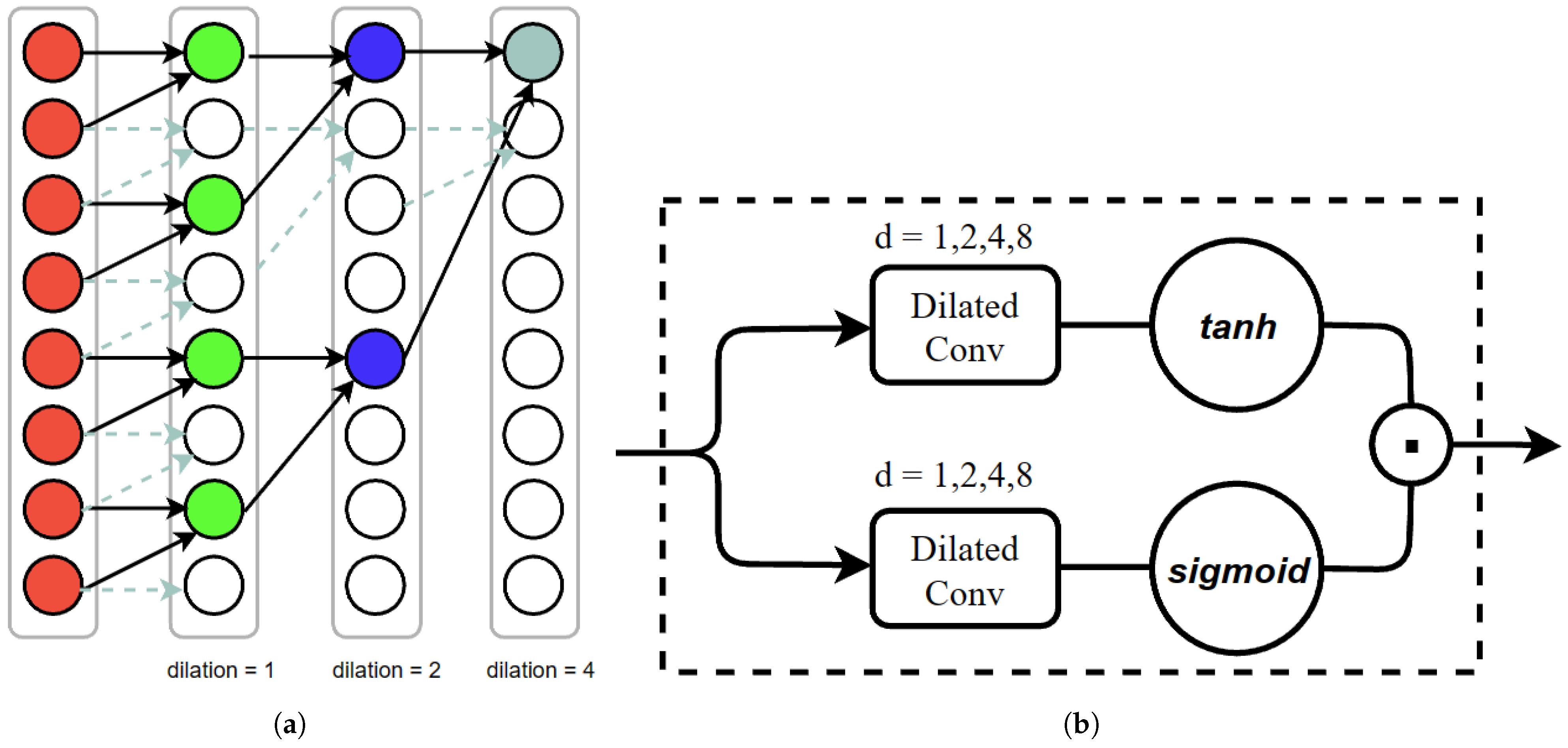
The fundamental concept behind the temporal layer is based on dilated convolution. By incorporating dilated convolution, the model can effectively expand its receptive field while maintaining the sequential nature of data modeling. This allows the model to capture longer temporal feature patterns with fewer computational costs, thereby capturing temporal dependencies over a larger time span.

Dilated convolution is a convolutional operation. As shown in Figure 4a, during the convolution process, fixed-sized “holes” are introduced between the elements of the convolution kernel, expanding the kernel. This means that, with the same computational cost, a larger effective filter size is used for convolution. Compared to a convolutional kernel of the same size, dilated convolution offers higher computational efficiency. In particular, dilated convolution with a dilation factor of 1 is equivalent to a regular convolution.

To accommodate different time step lengths, this paper adopts a dilation factor pattern of “1, 2, 4, 8” as the base and cycles through it as the model’s hidden layers increase. Let us apply this to the scenario of port traffic flow prediction, assuming that the input historical flow data have a time step length of 14 and the convolution kernel size is 3.

In the first layer of the temporal layer, the dilation factor is 1, which means that fine-grained time feature processing is performed at the level of 1 time step. As the network goes deeper, the second layer of the temporal layer has a dilation factor of 2; the process of applying time convolutions involves making leapfrog-like strides over the input sequence. This approach results in less fine-grained time feature processing, but, correspondingly, the same-sized convolutional kernel can handle twice the length of time steps.

By repeating this process, the temporal convolutional layer with a dilation factor of 8 can cover the entire input sequence, thereby extracting long-term historical features. This enables the model to capture temporal dependencies over a larger time span.

On the other hand, as a key to the success of recurrent neural networks, gating mechanisms preserve the non-linear capabilities while addressing the vanishing gradient problem, leading to better performance in tasks involving long-term dependencies. WaveNet [9] incorporates gating activation structures into causal convolutions, proposing the WaveNet structure shown in Figure 4b. The formula can be represented as

$$h_l\left(X\right)=tanh\left(X\ast W\right)\odot \delta (X\ast V)$$

(2)

where X represents the feature tensor, and l denotes the current layer. W and V represent two dilated convolution kernels, $\delta (\ast )$ represents the $sigmoid$ function, and ⊙ denotes the element-wise multiplication operator.

Based on this gating structure, the temporal layer can easily perform feature selection on the input data. Compared to linear processing methods, this nonlinear structure possesses stronger modeling capabilities for time series features.

2.3. Spatial Layer

The non-Euclidean nature, irregularity, and sparsity of graphs pose challenges in directly applying convolutional neural networks (CNNs) to process graph features. This limitation has impeded progress in graph representation within the field of machine learning. However, in recent years, researchers have made strides by combining spectral graph theory with Fourier transforms, allowing the definition of convolutional kernels in the spectral domain. This breakthrough has enabled graph convolutions in the spectral domain and has laid the foundation for graph convolutional networks (GCN) [12]. By simplifying the computation process, GCNs have facilitated rapid advancements in graph neural network models.

Subsequently, the graph attention network (GAT) [13] was proposed as a graph neural network model based on attention mechanisms. GAT controls the aggregation of information from nodes and edges by assigning different learning weights to their neighbors. This allows the model to extract more valuable hidden features. Compared to GCN, GAT offers a more flexible node feature aggregation process, addressing the limitation of GCN in which the fixed adjacency matrix prevents the graph structure from being expandable.

GAT can be divided into two stages: Stage 1 involves computing global similarity coefficients, while Stage 2 focuses on computing node features based on local attention coefficients.

Take a graph G = (V, E) with N port nodes as an example, where the historical flow features of each port can be represented as $X_i\in {\mathbb{R}}^{T\times C}$, with T being the time dimension and C being the feature dimension. In the graph attention layer, a trainable shared weight matrix W is first used to linearly transform the initial features of all nodes. Based on the edge relationships, the transformed node features are then used to calculate the similarity coefficients $e_{ij}$ between adjacent nodes on each edge. The formula for this stage is as follows, where N is the set of first-order neighboring nodes of the target node i, l is the current neural network layer, and the mapping function $a(\ast )$ is used to compute the similarity between the flow features of port nodes i and j.

$$e_{ij}^{\left(l\right)}=a\left(\left[W^{\left(l\right)}{X}_i^{\left(l\right)}\Vert W^{\left(l\right)}{X}_j^{\left(l\right)}\right]\right),j\in {\mathcal{N}}_i$$

(3)

In the aggregation stage, the model uses $softmax$ to normalize the similarity coefficients of all nodes within the first-order neighborhood of the target node i. The normalized coefficients represent the attention coefficients for each node within the neighborhood. The specific formula for the calculation of the attention coefficients is as follows:

$${\alpha }_{ij}^{\left(l\right)}=\frac{exp\left(LeakyReLU\left(e_{ij}^{\left(l\right)}\right)\right)}{{\displaystyle \sum _{k\in {\mathcal{N}}_i}}exp\left(LeakyReLU\left(e_{ik}^{\left(l\right)}\right)\right)}$$

(4)

Subsequently, the features of each node are weighted and aggregated based on the calculated attention coefficients, resulting in the new feature $X_i^{\left(l\right)}$ of the central node i at layer l. Here, $\sigma (\ast )$ represents an optional activation function.

$$h_l\left(X_i\right)=\sigma \left(\sum _{j\in {\mathcal{N}}_i}{\alpha }_{ij}^{\left(l\right)}{W}^{\left(l\right)}{X}_j^{\left(l\right)}\right)$$

(5)

Repeating Formulas (4) and (5), we perform feature aggregation for all nodes in the graph, completing the processing of a GAT layer.

In summary, the overall calculation formula for the spatiotemporal block of the model can be summarized as follows:

$$h_l\left(X^{(l-1)}\right)=tanh\left(WaveNet\left(X^{(l-1)}\right)\ast W+b\right)\odot \delta \left(GAT\left(X^{(l-1)}\right)\ast V+c\right)$$

(6)

3. Scenario and Data Sources

The experimental dataset in this study consists of 2019 AIS data and global port geospatial data.

Firstly, we employed big data techniques to process the vast amount of raw AIS data. To ensure data accuracy, we cross-referenced the information with vessel Lloyds Register profiles and applied data cleaning techniques to eliminate erroneous data. Subsequently, we integrated the trajectory data with spatial boundary information from global port geospatial data. This integration enabled us to infer the departure and arrival details of vessels, resulting in the creation of a global vessel port origin–destination (OD) dataset for the year 2019. The dataset comprised 154,205 vessels, 2697 ports, and a total of 5,275,645 records. Finally, leveraging the origin and destination port IDs, along with the recorded arrival and departure times in the OD dataset, we calculated the daily inflow and outflow of vessels for each port. This enabled us to quantify the daily traffic volume of ships entering and leaving each port.

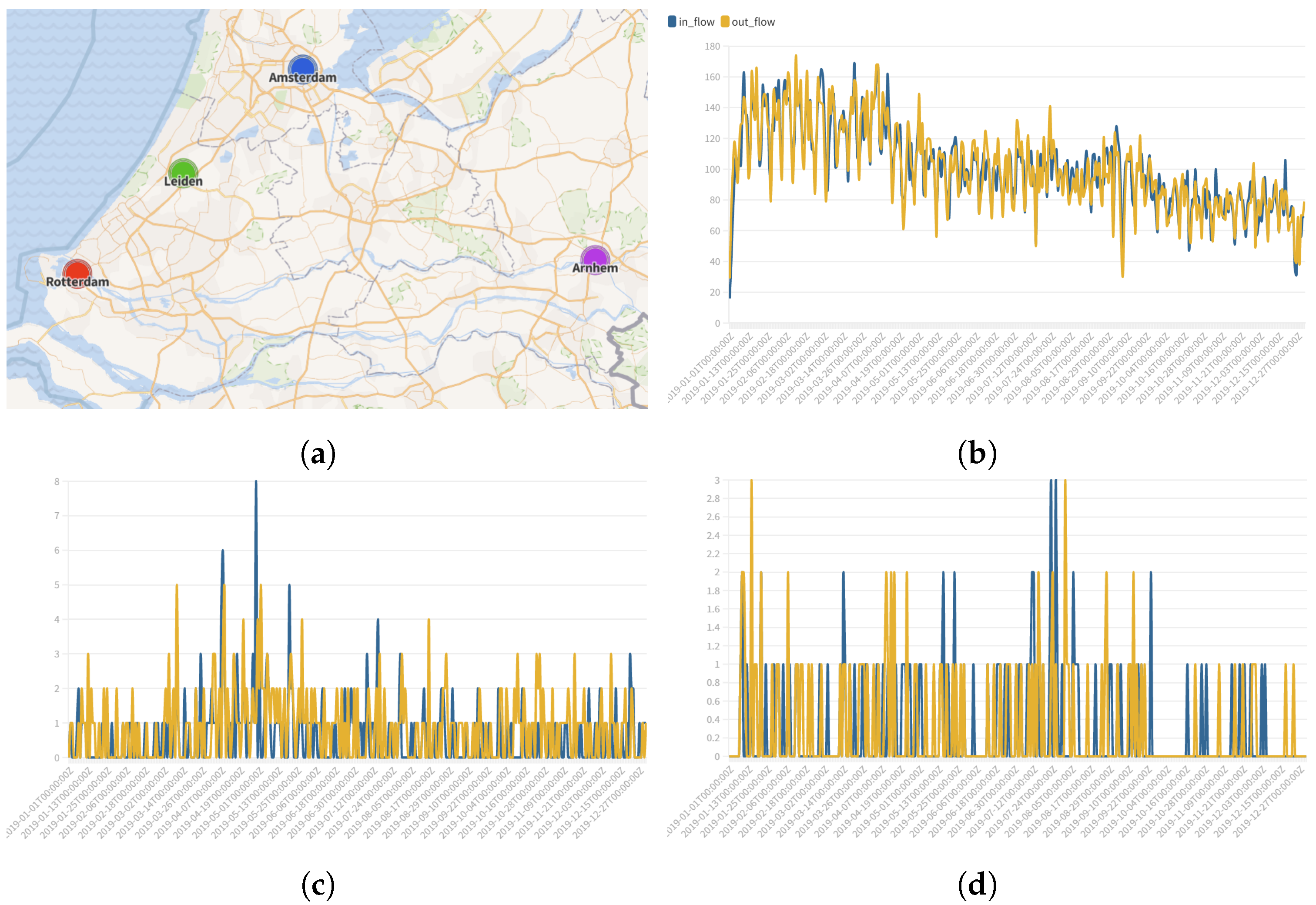
Following the acquisition of historical port traffic data, the creation of a multi-port spatial graph structure emerged as a pressing research challenge. Figure 5 illustrates that employing the physical distance alone as the basis for constructing the port graph structure would result in a significant loss of information. For instance, in the case of the Netherlands, Rotterdam Port exhibits considerably different average daily vessel traffic in comparison to nearby ports such as Leiden Port and Arnhem Port. This difference is also reflected in the scale of the ports, where Rotterdam Port is classified as a large-sized port with a maximum draught of 18 m, whereas Leiden Port and Arnhem Port fall under the category of medium-sized ports. Such disparities would introduce substantial errors during the feature aggregation stage within the graph convolutional layer.

To tackle this problem, the present study introduces a methodology for the construction of a dynamic port correlation graph utilizing historical data. The fundamental concept behind this approach is to employ actual maritime traffic patterns as an evaluative criterion. By quantifying the frequency of vessel movement between two ports, a spatial interconnection relationship is established, thereby creating an extensive multi-port correlation network.

Specifically, the initial step involves utilizing the previously generated 2019 global vessel port OD dataset, which is derived from the flow data calculation procedure, as the foundation for the construction of the graph. The direct count of vessel traffic between each pair of ports is computed on a monthly basis, encompassing global coverage. For the purpose of experimentation, three months of OD data are randomly selected for the computation process. A unidirectional edge relationship is established between two ports if the vessel traffic count surpasses a predefined threshold. In the experiment, this threshold was set to 10 to distinguish the level of closeness in the navigational relationship between two ports. To prevent the graph structure from becoming overly dense or sparse, we comprehensively consider the port scale and previous experiments, and determine the optimal range for this threshold as 5 to 10, guided by prior knowledge, which allows us to achieve the optimal solution in terms of computational costs and experimental effectiveness.

Moreover, taking into account the extensive number of ports globally and the substantial volume of OD data involved, we adopt a strategy to mitigate the computational overhead. This involves constructing independent sub-networks comprising port clusters, with several prominent ports across the world serving as central hubs. In our experiment, the central hubs selected were Rotterdam Port, Shanghai Port, Singapore Port, Boston Port, Antwerp Port, Hong Kong Port, and Incheon Port. This approach allows for the more efficient processing of the data while still capturing the essential connectivity among ports.

Using Rotterdam Port as an illustration, we initially filter the OD dataset to include only maritime shipping data where Rotterdam Port is either the origin or destination. We then identify the destination (or origin) ports that exhibit a mutual traffic count that satisfies the threshold constraint, thereby indicating direct connections to Rotterdam. Through this procedure, we identify a total of 250 port nodes that are directly linked to Rotterdam Port.

Subsequently, we shift our attention to these 251 ports and proceed to compute the direct vessel traffic count between each pair of ports. Employing a similar methodology as before, if the traffic count surpasses the predefined threshold, a unidirectional edge relationship is established between the two ports.

Finally, we obtain a sub-network structure comprising multiple ports, with Rotterdam Port as the central hub. The corresponding adjacency matrix is generated as a result. Figure 6 provides a visual representation of the schematic diagram depicting the multi-port graph structure centered around Rotterdam Port.

The geographical coordinates and location information of the seven central ports are displayed in Figure 7. The comprehensive data attributes of the port cluster network scene, centered around these seven ports, are recorded in

Table 1. Dataset attributes for seven port subnetworks.

Central Port Name	Port Nodes	Edges	Data Size
Rotterdam	251	3036	91,615
Shanghai	241	10,876	87,965
Singapore	388	10,017	141,620
Boston	121	1054	44,165
Antwerp	217	2706	79,205
Hong Kong	182	7731	66,430
Incheon	86	2733	31,390

.

4. Results

4.1. Experimental Environment

This study utilized a 2080ti GPU to conduct the experiments. To ensure a fair and consistent testing environment, the experiments were conducted on the Libcity platform [32], utilizing standardized hyperparameter configurations, with the hidden feature dimensions uniformly set to 32. The input window for time series data was defined as 21, while the output window was set to 7, meaning that the models aimed to predict the future 7-day traffic changes based on the preceding 21 days of data.

Specifically, the models employed in the study consisted of eight hidden layers. For models incorporating the multi-head attention mechanism, eight heads were used. In the case of models employing the diffusion convolution mechanism, the dilated factors were cyclically set as “1, 2, 4, 8”.

4.2. Baseline and Metric

In the experiment, the baseline models were divided into two major categories, spatiotemporal graph models and temporal models, based on whether they handled spatial features. RNN, AE [33], Seq2Seq [34], WaveNet [9], and Transformer [10] are classical temporal prediction methods that have proven effective in various domains, such as NLP and traffic prediction. STGCN [18], AGCRN [35], and the proposed model GAGW in this paper belong to spatiotemporal graph models. On the other hand, based on different time layer processing strategies, models can be further categorized into RNN-based prediction models led by RNN and DCRNN [21], TCN models such as GWNET [36] and STMGAT [37], and self-attention-mechanism-based models such as STTN [38].

The evaluation metrics used in the experiment include commonly employed measures in traffic flow prediction, MAE, MAPE, and RMSE, as depicted in Equations (7)–(9), respectively. MAE, known as the mean absolute error, is a widely used performance metric in regression tasks, directly quantifying the average difference between predicted values and actual values. MAPE, built upon MAE, measures the average percentage error of the experimental results. RMSE, or the root mean square error, in comparison to MAE, is more sensitive to large errors, thus challenging the stability and robustness of the predictive model.

$$MAE=\frac{1}{n}\sum _{i=1}^n\left|{\widehat{y}}_i-y_i\right|$$

(7)

$$MAPE=\frac{1}{n}\sum _{i=1}^n\left|\frac{\widehat{y_i}-y_i}{y_i}\right|\ast 100\%$$

(8)

$$RMSE=\sqrt{\frac{1}{n}\sum _{i=1}^n{\left({\widehat{y}}_i-y_i\right)}^2}$$

(9)

4.3. Experimental Results

In the experiment, we extracted the consecutive 21-day inflow and outflow data for each port from the test set as input and expected the model to generate predictions for the next 7 days of each port in a single output. Taking the Rotterdam sub-scenario as an example, which comprises 251 port nodes, the input should include an adjacency matrix with 251 nodes and an initial tensor of shape [32, 251, 21, 2]. Here, “32” represents the specified batch size, and “2” indicates that the initial features only include inflow and outflow. Correspondingly, the model’s output should be a tensor of shape [32, 251, 7, 2]. By comparing the predicted 7-day traffic variations with the ground truth values, the predictive capability of the model can be evaluated.

As presented in

Table 2. Results of multi-port dataset.

	Rotterdam			Boston			Antwerp			Hong Kong
	MAE	MAPE	RMSE	MAE	MAPE	RMSE	MAE	MAPE	RMSE	MAE	MAPE	RMSE
RNN	4.5813	0.6493	23.1354	3.2588	0.6722	6.4718	2.5007	0.6392	4.9709	16.3516	1.0782	33.7049
Auto Encoder	4.084	1.1835	11.4571	3.2034	0.625	6.3242	2.3923	0.6687	4.4949	18.3066	1.7544	32.9607
Seq2Seq	4.8228	0.6932	24.695	3.3392	0.6943	6.7335	2.4829	0.6209	5.0688	16.6819	0.9056	33.5273
WaveNet	2.5465	0.4315	9.4552	2.2362	0.4396	4.1007	1.8745	0.5385	3.2237	8.6431	0.432	18.5065
Transformer	2.5101	0.4891	8.401	2.1902	0.473	3.79	2.0819	0.5873	3.8074	8.5305	0.4564	17.6556
STGCN	3.2307	0.7186	9.5492	2.2647	0.498	3.9539	2.1825	0.5937	3.6725	13.1973	0.9862	27.4965
AGCRN	3.2396	0.5869	13.6182	2.5493	0.5111	4.7692	2.0179	0.5207	3.6471	9.8796	0.5501	21.5886
DCRNN	2.8718	0.616	9.8986	2.1044	0.4462	3.8234	1.7907	0.4909	3.191	8.9693	0.5549	18.5956
STTN	3.8664	0.6449	12.9845	2.2696	0.4827	4.0493	2.3098	0.5858	4.1153	16.9211	0.9443	33.6544
STMGAT	2.762	0.5231	8.6171	2.2309	0.4816	3.8571	1.7959	0.5038	3.0626	9.0416	0.6927	17.7191
GWNET	2.4831	0.4498	9.0111	2.1861	0.4421	4.0143	1.9133	0.5216	3.4256	8.5496	0.4489	17.6672
GAGW	2.3964	0.4485	8.514	2.0983	0.434	3.7663	1.7669	0.4719	3.0236	8.216	0.4436	17.2679
	Shanghai			Singapore			Incheon
	MAE	MAPE	RMSE	MAE	MAPE	RMSE	MAE	MAPE	RMSE
RNN	18.1033	1.8698	36.8206	10.1521	0.8326	31.2282	18.4991	1.3141	37.6816
Auto Encoder	17.5539	1.8645	35.2272	8.5357	0.7448	24.0477	19.6817	1.8012	37.5785
Seq2Seq	14.8196	1.1846	29.9094	10.1913	0.8657	31.0303	19.0404	1.3452	40.7782
WaveNet	7.4423	0.4437	15.98	5.1619	0.5057	14.8807	8.7669	0.4229	19.9683
Transformer	7.5331	0.4567	15.9231	4.3012	0.4288	11.5323	8.5554	0.4245	18.5527
STGCN	11.8722	0.6802	25.1572	7.9983	1.8568	16.0688	11.8275	0.783	26.6319
AGCRN	8.5064	0.6398	17.7152	4.7981	0.5475	12.9965	9.6283	0.5119	20.6766
DCRNN	7.6933	0.6046	16.1944	4.8215	0.5592	12.6221	8.9704	0.5052	19.4997
STTN	14.6455	1.1332	30.7543	9.279	0.8025	25.8419	19.6088	1.2163	40.3185
STMGAT	7.6263	0.4518	15.718	4.9113	0.65	12.3215	9.7628	0.7354	19.699
GWNET	7.525	0.5259	16.2727	4.426	0.5077	11.8064	9.4297	0.4956	22.2984
GAGW	7.306	0.4418	15.6874	4.3781	0.428	11.8228	8.7403	0.4672	19.8435

, cross-validation experiments were conducted across seven major multi-port network scenarios centered around the seven central ports. The GAGW model proposed in this study incorporates a weighted relationship to address the imbalance between spatial and temporal features. Consequently, the model demonstrates consistent and superior predictive performance across all scenarios, achieving the best results in the majority of experimental scenarios.

Through a comprehensive comparison of the experimental results, it has been observed that the majority of the existing spatiotemporal graph models outperform the temporal prediction models. This indicates that the incorporation of graph neural networks indeed enhances the performance of predictive models in various scenarios and effectively captures intricate traffic flow patterns. Among the temporal prediction models, Transformer and WaveNet exhibit significantly superior performance compared to traditional temporal prediction models and even outperform certain spatiotemporal graph models in specific scenarios. This highlights the significance of capturing temporal patterns in maritime traffic flow prediction scenarios, thereby affirming the importance of time features in the field of traffic prediction.

In the comparison of spatiotemporal graph models, the overall predictive performance of the STGCN model is relatively poor, which can be attributed to its use of a coarse-grained temporal processing strategy. The relatively simple gate convolution structure of STGCN is unable to fully capture the complex traffic flow variations in maritime scenarios, resulting in its performance being inferior to that of more sophisticated temporal prediction models such as Transformer.

In this experiment, the performance of the STTN model, which integrates self-attention mechanisms in both the temporal and spatial layers, did not meet our expectations. Despite adjusting certain hyperparameters, we were unable to obtain satisfactory experimental results. We speculate that the underlying reason for this lies in the spatial feature capturing strategy based on self-attention mechanisms. In the maritime context of this study, this strategy fails to effectively represent the data-driven, cross-spatial graph correlation structures, thereby leading to a decline in model performance.

The STMGAT, GWNET, and the proposed model in this paper all employ a time-convolution-based temporal layer processing strategy. The experimental results demonstrate that gate-based processing structures centered around causal convolutions can better capture the long-term variations in traffic flow data, enabling the fine-grained analysis of temporal features and obtaining more accurate prediction results.

The training curves of the top-performing three spatiotemporal graph models in the traffic flow scenario centered around the Rotterdam Port cluster are shown in Figure 8. The proposed model in this paper achieves more accurate predictive performance by utilizing a multi-head attention mechanism similar to STTN and STMGAT in the graph convolutional layer. However, this improvement in accuracy comes at the expense of sacrificing some training speed, resulting in a convergence speed that is not state-of-the-art. As illustrated in Figure 9, our model’s traffic flow predictions exhibit better adherence to the actual flow variation patterns compared to other baseline models and demonstrate good fitting capability for significant flow fluctuation curves.

To further investigate the stability of the model in the small-sample maritime test scenario, we extracted the traffic flow data from June to September as a specific monthly dataset for independent testing (

Table 3. Results of specific month dataset.

	Rotterdam			Boston			Antwerp			Hong Kong
	MAE	MAPE	RMSE	MAE	MAPE	RMSE	MAE	MAPE	RMSE	MAE	MAPE	RMSE
STGCN	10.0471	3.3148	19.1571	2.7766	0.558	5.0216	2.2405	0.5603	3.7479	21.7833	1.7334	44.5805
AGCRN	4.0285	0.5375	23.3363	2.7057	0.5186	5.118	2.0334	0.5032	3.7522	24.765	1.4236	53.009
DCRNN	6.7308	0.7575	36.2379	3.6936	0.5506	9.0707	3.5909	0.7169	9.1206	23.4573	1.6995	45.0641
STTN	7.3341	0.7816	37.1314	2.8498	0.508	5.6422	3.4785	0.6061	8.2283	25.1063	1.6549	50.5299
STMGAT	4.0649	0.5334	20.0261	2.7224	0.5165	5.0336	2.0679	0.4968	3.6653	18.2011	1.5736	39.1712
GWNET	3.62	0.5294	19.4332	2.7968	0.4875	5.3694	2.2134	0.5158	4.1839	14.0173	0.8861	31.1028
GAGW	3.3688	0.579	15.5115	2.6928	0.4753	5.0081	2.1446	0.5008	4.0861	13.3074	0.8242	29.6616
	Shanghai			Singapore			Incheon
	MAE	MAPE	RMSE	MAE	MAPE	RMSE	MAE	MAPE	RMSE
STGCN	21.8422	1.7012	45.8386	17.122	3.6693	36.7725	26.8699	1.8365	60.105
AGCRN	23.038	1.5282	47.7465	12.0759	0.9366	34.2086	21.9169	1.3855	44.5575
DCRNN	21.6196	1.8093	41.1723	14.5029	1.2927	39.0149	29.8365	1.6589	65.2048
STTN	22.5262	1.9444	44.5484	16.9381	1.2286	44.5798	23.6124	1.1277	59.0685
STMGAT	24.5565	2.6933	46.0391	6.9351	0.6712	19.7745	13.7049	0.6775	32.9118
GWNET	13.5886	0.9734	29.5113	6.9078	0.797	20.0405	15.5624	0.6453	40.8259
GAGW	11.9513	1.0716	26.2667	6.7402	0.6319	20.937	14.9141	0.6781	39.1262

). These four months are characterized by substantial fluctuations in port traffic, without a discernible pattern in the context of international shipping. Moreover, the navigation relationships among ports during this period are more intricate, placing higher demands on the predictive capabilities of the models. In this challenging scenario, the GAGW model stands out among numerous spatiotemporal prediction models and exhibits exceptional adaptability to the limited coverage of the specific monthly dataset. This further confirms the effectiveness of the new architecture.

To validate the issue of the unequal treatment of spatial and temporal features, we conducted ablation experiments by modifying some existing spatiotemporal graph model architectures to incorporate the proposed gate-based mechanism for spatiotemporal feature fusion. The experimental results, as shown in

Table 4. Ablation experiment on spatiotemporal feature fusion module.

	w/o Feature Fusion			w/Feature Fusion
	MAE	RMSE	R2	MAE	RMSE	R2
STGCN	13.7484	23.7532	0.9145	11.9819	21.2891	0.9319
STTN	21.6699	36.0566	0.8089	18.8857	33.1819	0.8384
GWNET	10.2954	20.1326	0.9402	10.3233	19.8169	0.943
ASTGCN	13.0184	22.8163	0.9229	11.3801	21.2428	0.9346
GAGW	10.9752	20.2516	0.9385	10.194	19.691	0.9428

, indicate that the spatiotemporal graph models with the inclusion of the feature fusion structure generally outperform the models with the original architectures in the port traffic prediction scenario of this paper. Among them, since the baseline models AGCRN and DCRNN both belong to iterative architectures based on RNN, it is difficult to incorporate the fusion module. Therefore, we introduced the ASTGCN [39] model, which simultaneously uses attention mechanisms and temporal convolution strategies, as the new baseline model.

To validate the relationship weights between time and spatial features, we conducted ablation experiments on the temporal and spatial layers of the GAGW model. In

Table 5. Ablation experiment of temporal and spatial layers.

	MAE	RMSE	R2
w/o T	12.5244	21.3558	0.9323
w/o S	10.2882	20.0338	0.9406
GAGW	10.1879	19.9007	0.9412

, “w/o T” represents the removal of all temporal hidden layers in the model, while “w/o S” indicates the removal of all graph structure processing methods. The experimental results demonstrate that ablating the temporal layer has a more severe impact on spatiotemporal graph models, leading to a significant decrease in predictive performance. In comparison, the performance decline is relatively limited when the spatial layer is ablated, further confirming the inequality between time and spatial features.

To demonstrate the superior performance of the proposed model in traffic flow prediction, we also conducted experiments on METR_LA, which is a renowned dataset comprising urban highway traffic speed data. As shown in

Table 6. Results of METR_LA.

METR_LA	RNN	AE	Seq2Seq	WaveNet	Transformer	STGCN	AGCRN	DCRNN	STTN	STMGAT	GWNET	GAGW
MAE	4.11	4.53	3.71	3.98	3.81	3.86	3.19	3.12	3.49	4.15	3.17	3.12
RMSE	8.17	8.77	7.19	8.98	8.73	8.34	6.33	6.19	7.92	8.24	6.39	6.11

, the GAGW model performs at an advanced level in the urban traffic dataset as well. This confirms that the phenomenon of unequal treatment between time and spatial features also exists in urban traffic scenarios.

In summary, the proposed model has demonstrated strong predictive capabilities in various experiments conducted in the multi-port traffic flow prediction scenario.

5. Conclusions

In this study, a comprehensive dataset of real port traffic and a port topology structure were constructed using global AIS data, Lloyd’s ship archive, and port geospatial data. To explore different modeling approaches, a variety of comparative models were reproduced using an open-source spatiotemporal graph model training framework [32].

Subsequently, a novel fine-grained multi-port traffic flow prediction spatiotemporal graph network model called GAGW was designed and implemented. This new model aimed to address the challenge of imbalanced temporal and spatial hidden features. Drawing inspiration from gate-based structures, the GAGW model processed temporal and spatial features in parallel, departing from the traditional sequential “time–space–time” processing pattern. The model incorporated distinct mapping functions for temporal and spatial feature vectors, placing greater emphasis on the influence of temporal features on prediction outcomes while reducing the sensitivity to spatial features.

To evaluate the effectiveness of the GAGW model, comparative experiments were conducted using maritime datasets, special monthly datasets, and urban road datasets. The results demonstrated the reliability and robustness of the proposed model. The GAGW model achieved advanced levels of prediction performance and robustness, among other evaluation metrics.

Overall, this research contributes to the field of port traffic flow prediction by introducing a novel spatiotemporal graph model that effectively handles imbalanced temporal and spatial features. The proposed GAGW model demonstrates superior prediction performance and adaptability, making it a promising approach for multi-port traffic forecasting applications.

Although the new framework has demonstrated the inequality of spatiotemporal features in experiments, there is room for further improvement in the construction of dynamic port graph structures. The proposed method for dynamic graph construction solely considers the spatial correlation between ports based on ship traffic, without incorporating the objective geographical relationships that exist between ports. In future work, the paper aims to focus on constructing flow datasets that encompass multi-port scenarios of practical significance, such as Europe and coastal regions of China.

Additionally, this paper only utilized AIS source data from the year 2019, which may be considered insufficient in capturing the full variability in port traffic patterns at a daily level. In future research, the study intends to incorporate AIS data from multiple consecutive years to augment the volume of data available for model training.

In summary, the future research endeavors of this paper will concentrate on two main aspects: optimizing the design of dynamic graph structures and refining the strategies for the processing of temporal layers in the model.