Robust Model Predictive Control Based on Active Disturbance Rejection Control for a Robotic Autonomous Underwater Vehicle

Abstract

This work aims to develop a robust model predictive control (MPC) based on the active disturbance rejection control (ADRC) approach by using a discrete extended disturbance observer (ESO). The proposed technique uses the ADRC approach to lump disturbances and uncertainties into a total disturbance, which is estimated with a discrete ESO and rejected through feedback control. Thus, the effects of the disturbances are attenuated, and a model predictive control is designed based on a canonical model free of uncertainties and disturbances. The proposed control technique is tested through simulation into a robotic autonomous underwater vehicle (AUV). The AUV’s dynamic model is used to compare the performance of a classical MPC and the combined MPC-ADRC. The evaluation results show evidence of the superiority of the MPC-ADRC over the classical MPC under tests of reference tracking, external disturbances rejection, and model uncertainties attenuation.

1. Introduction

Model predictive control (MPC) is based on the solution of an optimal control problem (OCP) for a prediction time horizon, subject to dynamic, states, and control constraints. The OCP attempts to find the best control sequence that produces the plant’s desired behavior. It is solved at every sample time step, taking as initial conditions the system’s current state. Then, the first element of the optimal control sequence is applied to the plant, and the entire optimization process is repeated at the subsequent sampled step with a moving horizon [1]. MPC was initially developed to meet the needs of industrial processes with relatively slow dynamics [2]; however, the development of computation capabilities of modern computers has impulsed the application of MPC to faster dynamic systems with complex dynamics. This is the case of MPC applied to autonomous underwater vehicles (AUV) [3,4], where the possibility to plan a control action according to the operation horizon’s features allows for the development of an anticipated control action instead of reactive control strategies.

MPC has been successfully implemented in a wide variety of applications; however, its main drawback is that it relays on the prior knowledge of an accurate mathematical model of the system dynamics. Variations of the classical MPC have been proposed to attenuate the effect of model uncertainties with techniques of robust MPC for linear systems [5]. Likewise, the robust nonlinear MPC (NMPC) have been proposed with the use of extended Kalman filters that estimate the process noise [6]. Robustness against model mismatching or unknown disturbances in NMPC are generally considered as an inherent property [7,8].

Most robust NMPC schemes that consider model uncertainties in the design process are based on minimizing the worst-case scenario from a set of uncertain models; however, the application of these techniques results in a complex task due to the need to impose stability constraints that could lead to an unfeasible solution during the search of an optimal control sequence [9]. In a complementary way, the adaptive model predictive control uses parametric estimation combined with robust MPC algorithms to gradually reduce the conservative control laws by adjusting the prediction model [10].

An alternative way to get a robust MPC is the estimation of disturbances through disturbance observers as high-gain observers [11], sliding mode disturbance observers [12], and nonlinear disturbance observers [13]. Although the disturbance observers in combination with predictive control have shown satisfactory results, their combination requires accurate prediction models and the evaluation of complex dynamic constraints. Alternatively, this paper proposes a model predictive control based on the active disturbance rejection control, which uses a discrete extended state observer to estimate the effects of model uncertainties and external disturbance. Additionally, the proposed control strategy uses a canonical dynamic model to predict the system behavior during the prediction horizon, which results in linear dynamic constraints.

Classical model-based control approaches rely on an accurate dynamic model of the system. However, in applications such as AUVs control, it is almost impossible to find a precise model, due to the hydrodynamic effects and the ocean flow currents, which produce model uncertainties and unknown external disturbances. Researchers have devoted a huge amount of effort to solving this problem. For instance, a sliding mode control (SMC) combined with an optimal thrust distribution on an over-actuated AUV was adopted to improve the robustness of dynamic positioning under the effects of the ocean current and model uncertainties [14]. The SMC has been also combined with disturbance observers to stabilize an AUV under time-varying external disturbance [15]. However, the SMC implementation needs to take special care of chattering in the control signals. Recently, adaptive control techniques based on backstepping have been developed for trajectory tracking task in AUVs [16,17]. The adaptive control approach has been also studied using fuzzy techniques with the design of fuzzy disturbance observer [18]. The use of disturbance observers has shown to be beneficial for the attenuation of disturbance effects. This is the case of the motion control strategy that integrates deep reinforcement learning and the extended state observer (ESO) to compensate for the model uncertainties into an optimal motion control policy [19]. Although the previously-mentioned controllers have effectively improve the closed-loop robustness of AUV motion control, there are opportunities to enhance the design process and results of control strategies for AUV. This is the case of combination of optimal control techniques like MPC with active disturbance rejection control strategies [20].

The remainder of this paper is organized as follows: The Section 2 describes the proposed control technique. Section 2.1 shows the design of the discrete extended state observer. Section 2.2 presents our proposed model predictive control based on the active disturbance rejection control approach. Section 2.3 finds a mathematical model for the autonomous underwater robot. Section 3 presents and discuses simulation results. Finally, Section 4 draws conclusions and future work.

2. Materials and Methods

The proposed control technique is a compound strategy that uses the features of a disturbance observer and an optimal control approach to finding a control sequence for a receding horizon that predicts the best control actions in every sampled time step. To develop the proposed technique, this section presents first a discrete extended state observer that estimates the system’s states and a total disturbance that lumps the external disturbances and model uncertainties into a single signal. Then, a model predictive control (MPC) strategy based on the active disturbance rejection control (ADRC) approach is developed for a general system with a single input and a single output. Then, an autonomous underwater vehicle is modeled to describe the dynamics of an underactuated underwater robot, which is based on the four DoF Seabotix LBV150 ROV. This model is transformed to separate the controllable dynamics from the uncontrollable internal dynamics of the system. This results in a simplified canonical model that is used to test the proposed MPC based on ADRC.

2.1. Discrete Extended State Observer

Let us consider a general nonlinear system, defined as

$$y_m^{\left(n\right)}=f_m\left(y_m,{\dot{y}}_m,\cdots ,y_m^{(n-1)}\right)+g_m\left(y_m,{\dot{y}}_m,\cdots ,y_m^{(n-1)}\right)u_m+\phi \left(y_m,{\dot{y}}_m,\cdots ,y_m^{(n-1)},u_m\right)+\zeta ,$$

(1)

where n is the order of the system, $y_m$ is the control output, $y_m^{\left(n\right)}$ is the n-th time derivative of $y_m$, $u_m$ is the control input, $f_m(·)$ is the known dynamic model of the system, $\phi (·)$ represents the model uncertainties and unmodeled dynamics, and $\zeta$ represents the external disturbances.

Assuming bounded uncertainties, bounded disturbances, and bounded dynamic behavior, the signals $\phi (·)$, $\zeta$, and $f_m\left(·\right)$ can be lumped into a total disturbance ${\xi }_m$, such as that (1) is transformed into

$$y_m^{\left(n\right)}=g_m\left(y_m,{\dot{y}}_m,\cdots ,y_m^{(n-1)}\right)u_m+{\xi }_m.$$

(2)

Then, a local approximation around a defined operation condition allows to express $g\left(·\right)$ as a constant ${\kappa }_m$, which is valid in an open neighborhood around the operation point. Then, (2) is expressed as,

$$y_m^{\left(n\right)}={\kappa }_m{u}_m+{\xi }_m.$$

(3)

This simplified model is used to design the extended state observer and feedback controller under the following assumptions:

Assumption 1.

The internal model of ${\xi }_m$ can be approximated by a constant, at least during an infinitesimal period of time.

Assumption 2.

${\xi }_m$ and its first time derivative are bounded.

Assumption 3.

The first time derivative of the total disturbance is expressed as

$$\frac{d}{dt}{\xi }_m=ϵ,$$

(4)

where ϵ is a small constant, such as that $ϵ\approx 0$.

Then, based on such assumptions, the variable ${\xi }_m$ can be used as an extended state of the dynamic system. This allows to define an extended state vector

$$\mathbf{x}:={[y_m{\dot{y}}_m{\ddot{y}}_m\cdots y_m^{(n-1)},{\xi }_m]}^{⊺},$$

(5)

which produces an extended state space representation of the system as

$$\begin{array}{ccccc}\hfill {\dot{y}}_m& =& {\dot{x}}_1\hfill & =& x_2,\hfill \\ \hfill {\ddot{y}}_m& =& {\dot{x}}_2\hfill & =& x_3,\hfill \\ \hfill ⋮& =& ⋮\hfill & =& ⋮\hfill \\ \hfill y_m^{\left(n\right)}& =& {\dot{x}}_n\hfill & =& x_{n+1}+\kappa u,\hfill \\ \hfill {\dot{\xi }}_m& =& {\dot{x}}_{n+1}\hfill & =& ϵ.\hfill \end{array}$$

(6)

In a compact form, the extended model is represented by a linear state space model given by:

$$\begin{array}{ccc}\hfill \dot{\mathbf{x}}& =& A\mathbf{x}+Bu+E,\hfill \\ \hfill y& =& C\mathbf{x},\hfill \end{array}$$

(7)

where $A\in {\mathbb{R}}^{(n+1)\times (n+1)}$, $B\in {\mathbb{R}}^{n+1}$, $C\in {\mathbb{R}}^{n+1}$, $E\in {\mathbb{R}}^{n+1}$,

$$A=\left[\begin{array}{ccccc}0& 1& 0& \cdots & 0\\ 0& 0& 1& \cdots & 0\\ ⋮& ⋮& ⋮& \ddots & ⋮\\ 0& 0& 0& \cdots & 1\\ 0& 0& 0& \cdots & 0\end{array}\right],B=\left[\begin{array}{c}0\\ 0\\ ⋮\\ \kappa \\ 0\end{array}\right],E=\left[\begin{array}{c}0\\ 0\\ ⋮\\ 0\\ ϵ\end{array}\right],C^{⊺}=\left[\begin{array}{c}1\\ 0\\ ⋮\\ 0\\ 0\end{array}\right].$$

Now, let us define a sampling period T and use the Euler’s method to find a discrete approximation of the extended linear model (7). This is,

$$\begin{array}{ccc}\hfill \mathbf{x}(k+1)& =& (I+TA)\mathbf{x}\left(k\right)+TBu\left(k\right)+TE,\hfill \\ \hfill y\left(k\right)& =& C\mathbf{x}\left(k\right),\hfill \end{array}$$

(8)

where k represents the discrete time variable.

Based on the discrete approximation of the simplified dynamic model (8), a  discrete extended state observer (ESO) is proposed using the Luenberger’s observer form. In this case, the observer estimates the system states, but also the total disturbance represented by the extended state $x_{n+1}$. Since the pair $(I+TA,C)$ is observable, the discrete ESO is proposed as follows:

$$\begin{array}{ccc}\hfill \widehat{\mathbf{x}}(k+1)& =& (I+TA)\widehat{\mathbf{x}}\left(k\right)+TBu\left(k\right)+L\left(y\left(k\right)-\widehat{y}\left(k\right)\right),\hfill \\ \hfill \widehat{y}\left(k\right)& =& C\widehat{\mathbf{x}}\left(k\right),\hfill \end{array}$$

(9)

where $\widehat{(·)}$ denotes the estimated variable and $L:={[l_1{l}_2\cdots l_n]}^{⊺}$ is the vector of the observer’s gains.

By subtracting (9) from (8), the estimation error dynamics is given by

$$\widehat{\mathbf{e}}(k+1)=(I+TA-LC)\widehat{\mathbf{e}}+TE,$$

(10)

where $\widehat{\mathbf{e}}:=\mathbf{x}-\widehat{\mathbf{x}}$.

Under the assumption of a bounded and small $ϵ$, the stability of (10) depends of the eigenvalues of $(I+TA-LC)$. Then, the observer gains are selected in such a way that the eigenvalues of $(I+TA-LC)$ are inside a unitary circle of a complex z-plane, which results in eigenvalues with modulus less than one. This ensures the convergence of the estimated states to the real ones and an accurate estimation of the total disturbance. This estimation will be used in the feedback control law proposed during the next section.

2.2. Robust MPC and ADRC

A model predictive control based on active disturbance rejection control is performed by using the disturbance estimation provided by the discrete ESO. The states and disturbance estimation are used into an optimal control problem (OCP) that computes an optimal control sequence for a receding horizon. The model used to predict the system behavior during the optimization process is a canonical structure that dismisses the model uncertainties, external disturbances, and model nonlinearities. This solves the optimization problem with less computation effort than the typical nonlinear MPC approaches. Since the total disturbance is rejected through feedback control, the result is a robust model predictive control strategy.

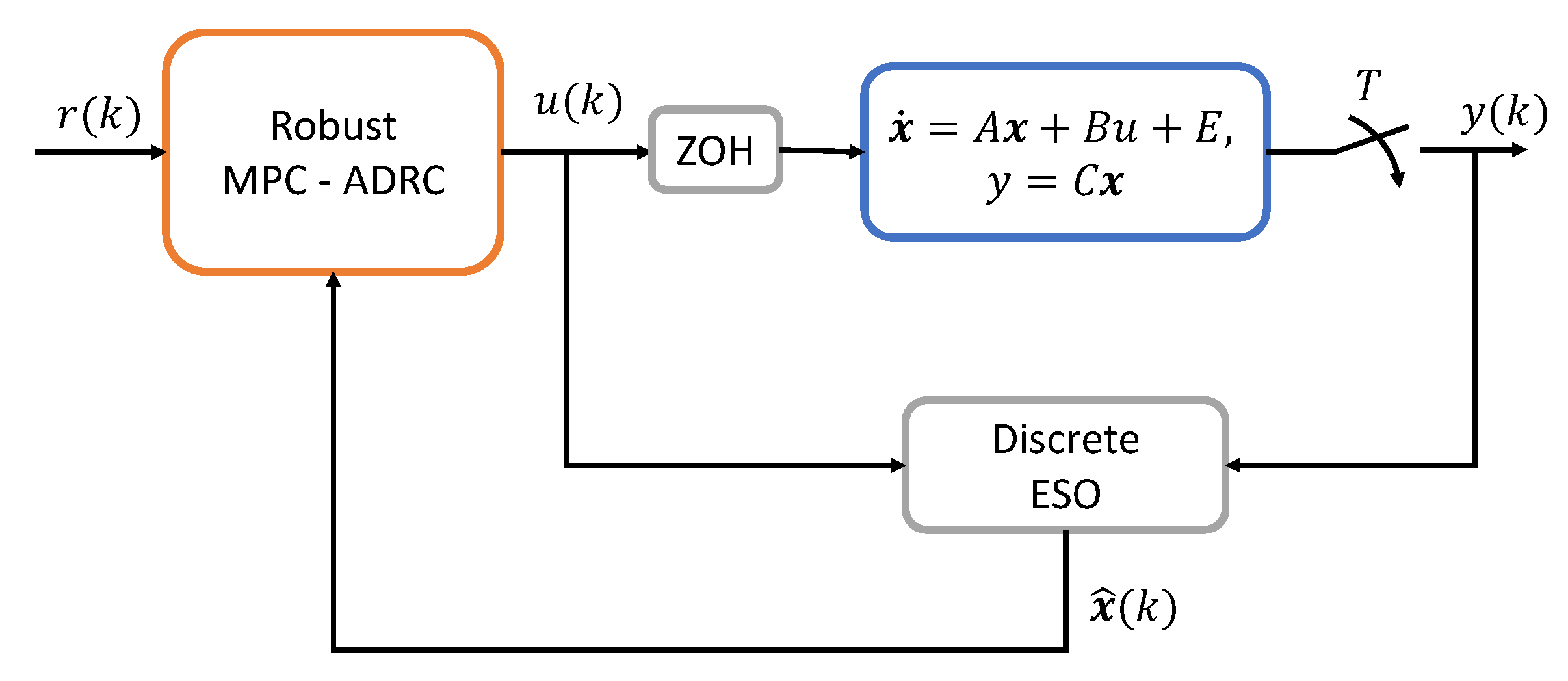
A general description of the control loop is shown into the Figure 1, where the continuous mathematical model represents the system dynamics, whose output y is sampled with a sampling period T. The sampled output $y\left(k\right)$ and control signal $u\left(k\right)$ are used by the discrete ESO to estimate the system states and the total disturbance, which are a source input to solve the OCP that produces the robust MPC-ADRC control law.

The OCP is defined to find an optimal control sequence that minimizes an objective function, which is projected in a time horizon into the future and computed based on a simplified model of the system. Based on the assumption that the total disturbance estimation converges to the real disturbance, the simplified model takes a canonical form that is used as a prediction model, which is almost free of uncertainties and disturbances. This canonical model is given by

$$\begin{array}{ccc}\hfill {\mathbf{x}}_s(k+1)& =& A_s{\mathbf{x}}_s\left(k\right)+B_s{u}_s\left(k\right),\hfill \\ \hfill y_s\left(k\right)& =& C_s{\mathbf{x}}_s\left(k\right),\hfill \end{array}$$

(11)

where ${\mathbf{x}}_s\left(k\right):={[y_m\left(k\right){\dot{y}}_m\left(k\right)\cdots y_m^{(n-1)}\left(k\right)]}^{⊺}$, $A_s\in {\mathbb{R}}^{n\times n}$, $B_s\in {\mathbb{R}}^n$, $C_s\in {\mathbb{R}}^n$,

$$A_s=\left[\begin{array}{cccc}1& T& \cdots & 0\\ ⋮& ⋮& \ddots & ⋮\\ 0& 0& \cdots & T\\ 0& 0& \cdots & 1\end{array}\right],B_s=\left[\begin{array}{c}0\\ 0\\ ⋮\\ T\kappa \end{array}\right],C_s^{⊺}=\left[\begin{array}{c}1\\ 0\\ ⋮\\ 0\end{array}\right].$$

In order to formulate the OCP, let us define, first, the control sequence along the prediction horizon, which will be considered as a vector of search variables in the optimization process. This is

$${\mathbf{u}}_s\left(k\right):={\left[u_s\left(0\right)u_s\left(1\right)\cdots u_s\left(\rho \right)\cdots u_s(N-1)\right]}^{⊺},$$

(12)

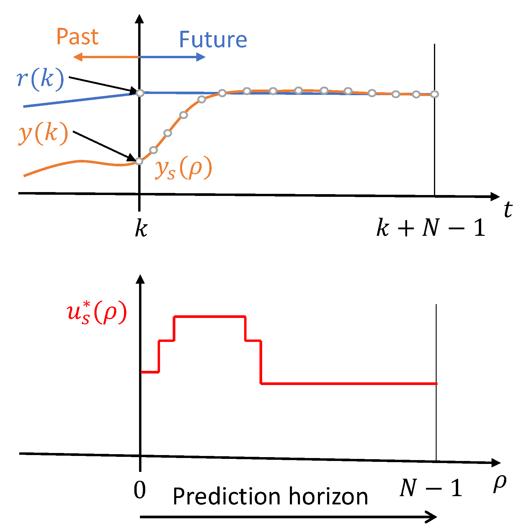
where N is the length, in samples, of the prediction horizon, $\rho \in {\mathbb{Z}}^{+}$ is the time discrete variable used inside the prediction horizon, which is set to zero in every sampling step and runs until $\rho =N-1$, this is $\rho =\{0,1,2,\cdots ,N-1\}$. The prediction horizon and control sequence are depicted into the Figure 2.

In the formulation of the optimal control problem, the cost function is defined as

$$J_N\left({\mathbf{u}}_s\left(k\right)\right)=\sum _{\rho =0}^{N-1}\left(w_e{e}_s^2\left(\rho \right)+w_u{u}_s^2\left(\rho \right)\right),$$

(13)

where $e_s\left(\rho \right):=r_s-y_s\left(\rho \right)$ is the tracking error, $r_s:=r\left(k\right)$ is the reference at time k, $w_e$ and $w_u$ are positive constant weights for the error and control signals, respectively.

The optimal control problem is subject to a set of equality and inequality constraints. The equality constraints ensure the satisfaction of initial conditions and the dynamic behavior of the system during the projected horizon. At the same time, the inequality constraints ensure that the control actions are inside of the actuators’ range of the action.

Then, the OCP is formulated as:

$$\begin{array}{ccc}\underset{{\mathbf{u}}_s\left(k\right)}{min}\hfill & \hspace{1em}\hspace{1em}\hspace{1em}\hspace{1em}\hspace{1em}{J}_N\left({\mathbf{u}}_s\left(k\right)\right)& \hfill \end{array}$$

(14)

$$\begin{array}{ccc}\mathrm{s}.\mathrm{t}.:\hfill & {\mathbf{x}}_s\left(\rho \right)={[{\widehat{x}}_1{\widehat{x}}_2\cdots {\widehat{x}}_n]}^{⊺},& \rho =0,\hfill \end{array}$$

(15)

$$\begin{array}{ccc}& {\mathbf{x}}_s(\rho +1)=A_s{\mathbf{x}}_s\left(\rho \right)+B_s{u}_s\left(\rho \right),& \forall \rho \in [0,N-1],\hfill \end{array}$$

(16)

$$\begin{array}{ccc}& -u_{max}+\frac{1}{\kappa }{\widehat{x}}_{n+1}\le u_s\left(\rho \right)\le u_{max}+\frac{1}{\kappa }{\widehat{x}}_{n+1},& \rho =0,\hfill \end{array}$$

(17)

$$\begin{array}{ccc}& -u_{max}\le u_s\left(\rho \right)\le u_{max},& \forall \rho \in [1,N-1],\hfill \end{array}$$

(18)

where (14) is the cost function, (15) sets the initial conditions of the model to the state values computed by the discrete ESO at time k, (16) is a dynamic constraint that ensures the satisfaction of the system dynamics based on the canonical model (11), (17) imposes boundaries for the control signal at the first time step of the prediction horizon, these bounds are modified every sampled time step according to the total disturbance estimation, in such a way that the optimal control sequence allows to inject the rejection of the estimated disturbance. Likewise, (18) establishes the boundaries for the control actions over the prediction horizon between $\rho =1$ and $\rho =N-1$.

The implementation of the dynamic constraints implies the propagation of the initial conditions through all the prediction horizon, which results in a complex nonlinear structure that increases the computation time. In order to reduce the complexity of the dynamic constraints, a multiple shooting approach is used to transform the dynamic propagation into a set of equality constraints [21].

In order to implement the multiple shooting algorithm, let us define an extended set of search variables in a vector as

$$\mathbf{w}:={\left[{\mathbf{u}}_s^{⊺}\left(k\right){\mathbf{x}}_s^{⊺}\left(0\right){\mathbf{x}}_s^{⊺}\left(1\right)\cdots {\mathbf{x}}_s^{⊺}\left(N\right)\right]}^{⊺},$$

(19)

where $\mathbf{w}$ includes the control and state vectors sequences at $t=k$. This search vector increases the number of search variables but simplifies the nonlinearity propagation of the system dynamics along the prediction horizon. Based on this approach, the system’s dynamic constraints are included as a set of equality constraints as

$${\mathbf{h}}_N\left(\mathbf{w}\right):=\left[\begin{array}{c}{\mathbf{x}}_s\left(0\right)-{[{\widehat{x}}_1{\widehat{x}}_2\cdots {\widehat{x}}_n]}^{⊺}\\ {\mathbf{x}}_s\left(1\right)-\left(A_s{\mathbf{x}}_s\left(0\right)+B_s{u}_s\left(0\right)\right)\\ ⋮\\ {\mathbf{x}}_s\left(N\right)-\left(A_s{\mathbf{x}}_s(N-1)+B_s{u}_s(N-1)\right)\end{array}\right]=\mathbf{0},$$

(20)

and a set of inequality constraints defined as

$${\mathbf{g}}_N\left(\mathbf{w}\right):=\left[\begin{array}{c}{u}_s\left(0\right)-u_{max}-\frac{1}{\kappa }{\widehat{x}}_{n+1}\\ u_s\left(1\right)-u_{max}\\ u_s\left(2\right)-u_{max}\\ ⋮\\ u_s\left(N\right)-u_{max}\\ -u_s\left(0\right)-u_{max}+\frac{1}{\kappa }{\widehat{x}}_{n+1}\\ -u_s\left(1\right)-u_{max}\\ -u_s\left(2\right)-u_{max}\\ ⋮\\ -u_s\left(N\right)-u_{max}\end{array}\right]\le \mathbf{0}.$$

(21)

Then, the OCP is transformed into a nonlinear programming problem (NLP) as

$$\begin{array}{ccc}\hfill {\displaystyle \underset{\mathbf{w}}{min}}& J_N\left(\mathbf{w}\right)& \\ \hfill \mathrm{s}.\mathrm{t}.:& {\mathbf{g}}_N\left(\mathbf{w}\right)\le \mathbf{0},& \mathrm{Inequality} \mathrm{constraints},\hfill \\ \hfill & {\mathbf{h}}_N\left(\mathbf{w}\right)=\mathbf{0},& \mathrm{Equality} \mathrm{constraints}.\hfill \end{array}$$

The solution of the NLP results in an optimal sequence of control actions and a set of state vectors that minimize the cost function for the prediction horizon. Based on that solution, the control action for the current sampled time k is computed by subtracting the total disturbance effect, which was estimated by the discrete ESO, from the first element of the optimal control sequence found in the NLP. This allows to define a control law as

$$u\left(k\right):=u_s^{*}\left(0\right)-\frac{1}{\kappa }{\widehat{x}}_{n+1}\left(k\right).$$

(22)

where ${\mathbf{u}}_s^{*}$ denotes the optimal control sequence and $u_s^{*}\left(0\right)$ is the first element of the sequence.

In order to compute the closed-loop behavior under the effect of the control signal proposed in (22), it is applied to the discrete model shown in (8), which results in a closed-loop dynamics describe by

$$\begin{array}{ccc}\hfill x_1(k+1)& =& x_1\left(k\right)+T{x}_2\left(k\right),\hfill \\ \hfill x_2(k+1)& =& x_2\left(k\right)+T{x}_3\left(k\right),\hfill \\ \hfill ⋮& =& ⋮\hfill \\ \hfill x_n(k+1)& =& x_n\left(k\right)+T\kappa u_s^{*}\left(0\right)+T\left(x_{n+1}\left(k\right)-{\widehat{x}}_{n+1}\left(k\right)\right),\hfill \\ \hfill x_{n+1}(k+1)& =& x_{n+1}\left(k\right)+Tϵ.\hfill \end{array}$$

(23)

The stability analysis of the closed-loop dynamics is divided into two parts. The first part considers the stability guaranteed by the selection of the ESO’s gains. The appropriate selection of ESO’s gains allows for defining an ultimate bound to the total disturbance estimation as

$$\underset{k\to \infty }{lim}\left(x_{n+1}\left(k\right)-{\widehat{x}}_{n+1}\left(k\right)\right)=\gamma ,$$

(24)

where $\gamma$ is a positive constant that can be arbitrarily reduced as much as the physical limitation in the hardware allows. The second part of the stability analysis considers the effect of the optimal control sequence ${\mathbf{u}}_s^{*}$. Since this control sequence is computed from a subset of control signals that guarantee the closed-loop stability through the convergence of the optimization problem system, then it is possible to affirm that the closed-loop is stable and the controlled variables converge to the vicinity of the target trajectory with an ultimate bound.

Finally, The a summary of the implementation procedure of the MPC based on ADRC is shown in the Algorithm 1. The following section shows the implementation of the algorithm on an autonomous underwater robot.

Algorithm 1: MPC-ADRC implementation

Step 0: Find a simulation model. Step 1: Design ESO. Step 1.1: Define the order of the design dynamic model n and find an approximation of the control input gain $\kappa$. Step 1.2: Build the extended state model with the canonical form described in (7). Step 1.3: Define a sampling period T according the Nyquist–Shannon sampling theorem and find a discrete model approximation of the system dynamics as (8). Step 1.4: Assign the observer gains L such as the eigenvalues of $I+TA-LC$ are inside the unite circle in the complex z-plane and build the extended state observer ESO as shown in (9). Step 2: MPC implementation. Step 2.1: Define the weights $w_e$ and $w_u$ and build the cost function (13). Step 2.2: Define the equality constraints (20) and inequalities constraints (21). Step 2.3: Define the prediction horizon length N. Step 2.4: Implement a nonlinear programming algorithm that solves the optimization problem at each sampling step. Step 3: Evaluation. Step 3.1: Build the control law as (22) and evaluate the closed-loop control using the simulation model. Step 3.2: Evaluate the performance and robustness of the closed-loop, if it is necessary change observer gains L, weights $w_e$ and $w_u$, or prediction horizon length N and repeat evaluation.

2.3. Autonomous Underwater Robot Model

In order to test the proposed robust MPC based on ADRC, an autonomous underwater robot is used as a test platform of the control strategy. This system has dynamic features that make it a suitable application of the robust MPC based on ADRC. First, the system dynamics is highly nonlinear with hydrostatic and hydrodynamic effects that difficult an accurate model identification. Second, the environment where the robot works has a high degree of uncertainty with unpredictable ocean currents, especially in the vicinity of reefs where the water flow is distorted by the rocks. These produce external disturbances on the robot dynamics, which must be rejected by the control system. A third reason to apply the proposed control strategy to the robotic AUV is the need to guarantee the satisfaction of safety constraints to avoid the collision of the robot with obstacles in the environment and to optimize the performance of the robot to increase its energy autonomy.

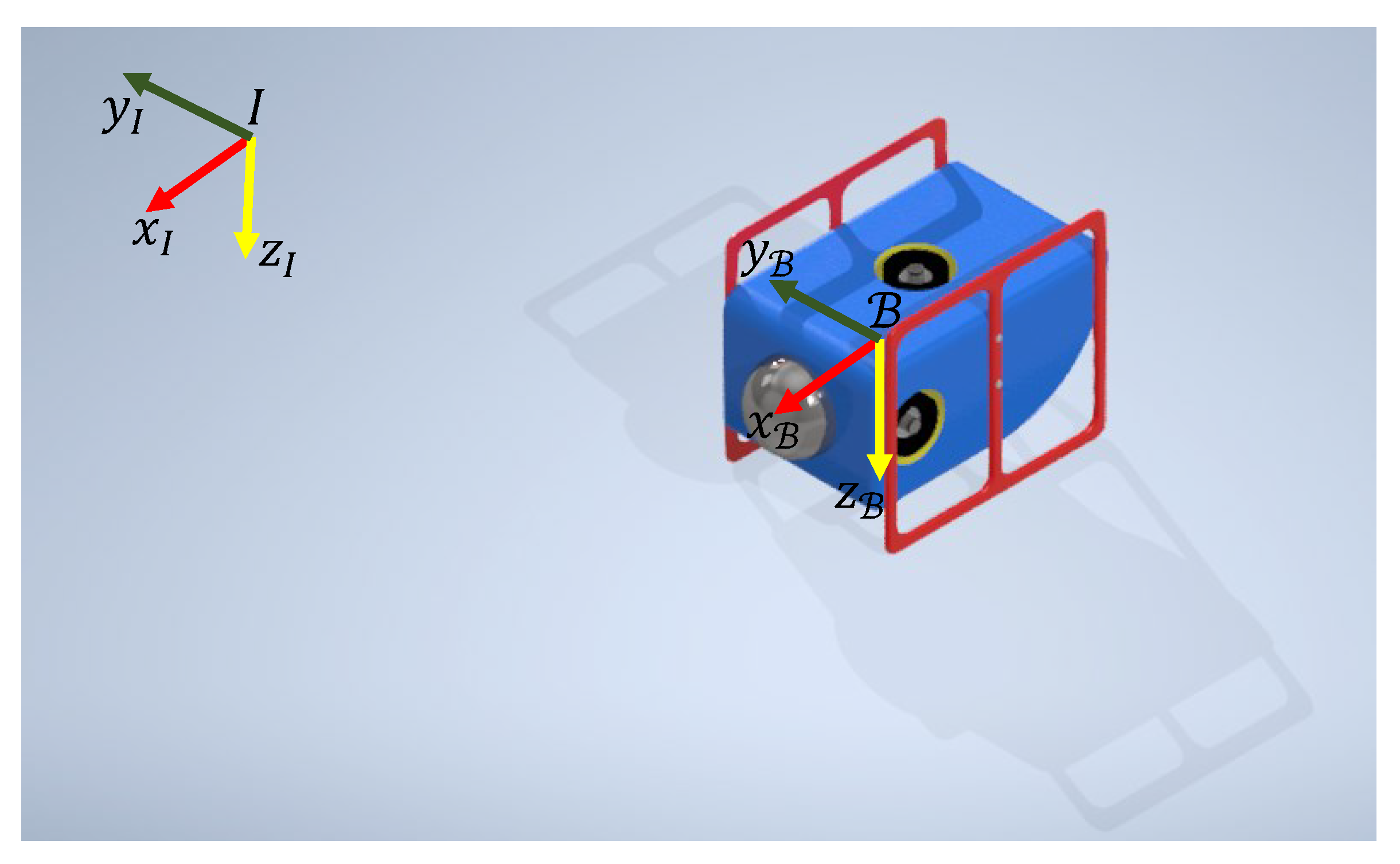
Let us consider the robotic autonomous underwater vehicle (AUV) shown in the Figure 3, which has four thrusters: two in the rear, one in the top, and one in the port (left side) [22]. The frames $\mathcal{I}$ and $\mathcal{B}$ shown in the figure represent the fixed inertial frame and the body frame, respectively.

In order to find a mathematical model that describes the dynamic behavior of the robotic AUV, the motion variables are defined according with the SNAME notation for a submerged body through a fluid [23]. In this sense, the position of the robot is defined as $\mathit{\eta }:={\left[{\mathit{\eta }}_1^{⊺}{\mathit{\eta }}_2^{⊺}\right]}^{⊺}$, where ${\mathit{\eta }}_1\in {\mathbb{R}}^3$ represents the position with respect to the inertial frame $\mathcal{I}$ and ${\mathit{\eta }}_2\in {\mathcal{S}}^3$ represents the robot’s attitude, as well known as pose. To describe the position of the robot, the three Cartesian coordinates are used such as that ${\mathit{\eta }}_1:={\left[xyz\right]}^{⊺}$, where x, y, and z represent the motion in the directions of surge, sway, and heave, respectively. Likewise, the attitude is represented with the Euler angles as ${\mathit{\eta }}_2:={\left[\varphi \theta \psi \right]}^{⊺}$, where $\varphi$, $\theta$, and $\psi$ represent roll, pitch, and yaw, respectively.

Then, the Newton-Euler’s method is used to analyze the motion of a submerged rigid-body with six degrees of freedom (DoF) [24]. The mathematical model that describes the AUV motion is given by

$$\begin{array}{ccc}\hfill \mathit{M}\dot{\mathit{\nu }}+\mathit{C}\left(\mathit{\nu }\right)\mathit{\nu }+\mathit{D}\left(\mathit{\nu }\right)\mathit{\nu }+\mathit{g}\left(\mathit{\eta }\right)& =& \mathbf{\Gamma },\hfill \end{array}$$

(25)

$$\begin{array}{ccc}\hfill \dot{\mathit{\eta }}& =& \mathit{J}\left(\mathit{\eta }\right)\mathit{\nu },\hfill \end{array}$$

(26)

where $\mathit{\nu }:={\left[{\mathit{\nu }}_1^{⊺}{\mathit{\nu }}_2^{⊺}\right]}^{⊺}\in {\mathbb{R}}^6$ denotes the linear and angular velocities with ${\mathit{\nu }}_1:={\left[uvw\right]}^{⊺}$ and ${\mathit{\nu }}_2:={\left[pqr\right]}^{⊺}$, respectively. $\mathbf{\Gamma }$ designates a vector of generalized forces and moments defined as: $\mathbf{\Gamma }:={\left[{\mathit{f}}^{⊺}{\mathit{\tau }}^{⊺}\right]}^{⊺}$, where the body-fixed forces in x, y, and z are represented as $\mathit{f}:={\left[XYZ\right]}^{⊺}$ and the body-fixed moments in $\varphi$, $\theta$, and $\psi$ are defined as $\mathit{\tau }:={\left[KMN\right]}^{⊺}$.

Since the submerged body is exposed to hydrostatic and hydrodynamic effects, the mass matrix includes the rigid body mass and inertial in ${\mathit{M}}_{RB}$, and an added mass term in ${\mathit{M}}_A$, which represents the mass of fluid surrounding the robot that it must move to deflect the resistance of the fluid. This is modeled as a virtual mass added to the rigid body as:

$$\mathit{M}:={\mathit{M}}_{RB}+{\mathit{M}}_A,$$

(27)

where ${\mathit{M}}_{RB}\in {\mathbb{R}}^{6\times 6}$ and ${\mathit{M}}_A\in {\mathbb{R}}^{6\times 6}$. Likewise, the Coriolis and centrifugal effects are represented as

$$\mathit{C}\left(\mathit{\nu }\right):={\mathit{C}}_{RB}+{\mathit{C}}_A,$$

(28)

where ${\mathit{C}}_{RB}\in {\mathbb{R}}^{6\times 6}$ designates the effects of the rigid-body and ${\mathit{C}}_A\in {\mathbb{R}}^{6\times 6}$ designates the effects of the added mass. An additional factor in the description of the AUV is the viscous damping. This is a hydrodynamic effect that produces dissipative moments and forces. The main sources of damping are the skin friction and the interaction with waves and internal currents. The total effects of damping are lumped into a drag matrix $\mathit{D}\left(\mathit{\nu }\right)$, which is approximated as

$$\mathit{D}\left(\mathit{\nu }\right):={\mathit{D}}_q\left(\mathit{\nu }\right)+{\mathit{D}}_l,$$

(29)

where ${\mathit{D}}_q\left(\mathit{\nu }\right)\in {\mathbb{R}}^{6\times 6}$ and ${\mathit{D}}_l\in {\mathbb{R}}^{6\times 6}$ are the quadratic and linear drag matrices, respectively.

The term $\mathit{g}\left(\mathit{\eta }\right)$ describes the restoring forces acting in the robot. It includes the gravitational effects represented by a force W passing through the center of gravity (CG) and a buoyancy force B passing through the center of buoyancy (CB). The restoring forces and moments are expressed in the body-fixed frame as

$$\mathit{g}\left(\mathit{\eta }\right)=\left[\begin{array}{c}(W-B)sin\theta \\ -(W-B)cos\theta sin\varphi \\ -(W-B)cos\theta cos\varphi \\ -(y_{g}W-y_{b}B)cos\theta cos\varphi +(z_{g}W-z_{b}B)cos\theta sin\varphi \\ (z_{g}W-z_{b}B)sin\varphi +(x_{g}W-x_{b}B)cos\theta cos\varphi \\ -(x_{g}W-x_{b}B)cos\theta sin\varphi -(y_{g}W-y_{b}B)sin\theta \end{array}\right],$$

(30)

where $W=mg$, $B={\rho }_{w}g\nabla$, m is the sum of the robot mass and the mass of water in the ballast tanks, g is the acceleration of the gravity, ${\rho }_w$ is the water density, ∇ is the volume of liquid displaced by the robot, $x_g$, $y_g$, $z_g$, and $x_b$, $y_b$, $z_b$, are the coordinates of the CG and CB with respect to the frame $\mathcal{B}$. In an effort to simplify the dynamic interaction between these two forces, the CG and CB are considered coincident in the origin of $\mathcal{B}$; however, in general, it is desirable to design AUV with the CB ahead of the CG to guarantee controllability and stability in pitch.

The Jacobian matrix $\mathit{J}\left(\mathit{\eta }\right)$ transforms the relative velocities expressed in $\mathcal{B}$ into the inertial reference frame $\mathcal{I}$. This is

$$\begin{array}{ccc}\hfill \dot{\mathit{\eta }}& =& \mathit{J}\left(\mathit{\eta }\right)\mathit{\nu },\hfill \end{array}$$

(31)

$$\begin{array}{ccc}& \Downarrow & \end{array}$$

(32)

$$\begin{array}{ccc}\hfill \left[\begin{array}{c}\dot{x}\\ \dot{y}\\ \dot{z}\\ \dot{\theta }\\ \dot{\varphi }\\ \dot{\psi }\end{array}\right]& =& \left[\begin{array}{cc}{\mathit{J}}_1\left({\mathit{\eta }}_2\right)& {\mathbf{0}}_{3\times 3}\\ {\mathbf{0}}_{3\times 3}& {\mathit{J}}_2\left({\mathit{\eta }}_2\right)\end{array}\right]\left[\begin{array}{c}u\\ v\\ w\\ p\\ q\\ r\end{array}\right],\hfill \end{array}$$

(33)

where ${\mathit{J}}_1\left({\mathit{\eta }}_2\right):=\mathbf{R}\left({\mathit{\eta }}_2\right)\in \mathcal{SO}\left(3\right)$ and ${\mathit{J}}_2\left({\mathit{\eta }}_2\right)\in {\mathbb{R}}^{3\times 3}$ are a rotational and a transformation matrices, respectively.

Since the underwater thrusters installed on the robot are not strictly aligned with the body-fixed frame axis, the propulsion forces do not produce a pure vector of generalized forces and moments in $\mathbf{\Gamma }$. Then, it is necessary to find a mathematical expression that relates the propulsion force vector ${\mathbf{f}}_{th}$ with the $\mathbf{\Gamma }$. This is

$$\mathbf{\Gamma }:=T_{th}{\mathbf{f}}_{th},$$

(34)

where $T_{th}$ is known as an allocation matrix, which depends on the robot’s architecture and the location of the thrusters. Additional details about the model can be found in [22,25].

Since the robot considered in this paper has four thrusters and can move in six DoF, then the system is underactuated. This implies that the robot is partially controllable and part of its dynamics is not directly affected by the propulsion of the actuators. According to the geometrical distribution of the thrusters, the robot is underactuated in the pitch and roll angles. Therefore, the following assumptions are adopted:

Assumption 4.

It is assumed that the dynamics of the underactuated DoF are stabilized with complementary elements such as fairwater planes.

Assumption 5.

High speed and sharp turns are avoided to evade instability effects in the vertical plane.

In order to adapt the proposed control strategy to the robotic AUV, a transformation of the model is executed such as that the nonlinearities, model uncertainties, and external disturbances are shown as input equivalent signals and the controllable dynamics is isolated from the uncontrollable one. First, let us write the model as general nonlinear system

$${\dot{\mathbf{x}}}_r={\mathbf{f}}_r\left({\mathbf{x}}_r\right)+{\mathbf{g}}_r{\mathbf{u}}_r+{\mathit{\zeta }}_r,$$

(35)

where ${\mathit{\zeta }}_r$ represents the unmodeled dynamics and external disturbances, ${\mathbf{x}}_r={\left[{\mathit{\eta }}^{⊺}{\dot{\mathit{\eta }}}^{⊺}\right]}^{⊺}$, ${\mathbf{u}}_r={\mathbf{f}}_{th}$,

$${\mathbf{f}}_r\left({\mathbf{x}}_r\right)=\left[\begin{array}{c}\dot{\mathit{\eta }}\\ \nabla \mathit{J}\left(\mathit{\eta }\right)\dot{\mathit{\eta }}+{\mathit{M}}^{-1}\left(-\mathit{C}\left(\mathit{\nu }\right)\mathit{\nu }-\mathit{D}\left(\mathit{\nu }\right)\mathit{\nu }-\mathit{g}\left(\mathit{\eta }\right)\right)\end{array}\right],{\mathbf{g}}_r\left({\mathbf{x}}_r\right)=\left[\begin{array}{c}0\\ {\mathit{M}}^{-1}{T}_{th}\end{array}\right],$$

and

$$\mathit{\nu }={\mathit{J}}^{-1}\left(\mathit{\eta }\right)\dot{\mathit{\eta }}.$$

Then, the control output is defined as:

$$\mathbf{h}\left({\mathbf{x}}_r\right):=\left[\begin{array}{c}{x}^{*}-x\\ y^{*}-y\\ z^{*}-z\\ {\psi }^{*}-\psi \end{array}\right],$$

(36)

where ${(·)}^{*}$ denotes the control reference.

By applying successive time derivatives to the control output until the control input is explicit, the system dynamics takes the form

$$\begin{array}{ccc}\hfill \frac{d}{dt}\mathbf{h}\left({\mathbf{x}}_r\right)& =& \nabla \mathbf{h}\left({\mathbf{x}}_r\right){\dot{\mathbf{x}}}_r,\hfill \end{array}$$

(37)

$$\begin{array}{ccc}\hfill \frac{d}{dt}\mathbf{h}\left({\mathbf{x}}_r\right)& =& \nabla \mathbf{h}\left({\mathbf{x}}_r\right){\mathbf{f}}_r\left({\mathbf{x}}_r\right),\hfill \end{array}$$

(38)

$$\begin{array}{ccc}\hfill \frac{d}{dt}\mathbf{h}\left({\mathbf{x}}_r\right)& =& {\mathbf{L}}_{{\mathbf{f}}_r}\mathbf{h}\left({\mathbf{x}}_r\right),\hfill \end{array}$$

(39)

$$\begin{array}{ccc}\hfill \frac{d^2}{d{t}^2}\mathbf{h}\left({\mathbf{x}}_r\right)& =& {\mathbf{L}}_{{\mathbf{f}}_r}^2\mathbf{h}\left({\mathbf{x}}_r\right)+{\mathbf{L}}_{{\mathbf{g}}_r}{\mathbf{L}}_{{\mathbf{f}}_r}\mathbf{h}\left({\mathbf{x}}_r\right){\mathbf{u}}_r+{\mathbf{L}}_{{\zeta }_r}{\mathbf{L}}_{{\mathbf{f}}_r}\mathbf{h}\left({\mathbf{x}}_r\right),\hfill \end{array}$$

(40)

where $\nabla \mathbf{h}\left({\mathbf{x}}_r\right)$ is the gradient of $\mathbf{h}\left({\mathbf{x}}_r\right)$, ${\mathbf{L}}_{{\mathbf{f}}_r}\mathbf{h}\left({\mathbf{x}}_r\right)$ is the Lie derivative of $\mathbf{h}\left({\mathbf{x}}_r\right)$ along ${\mathbf{f}}_r\left({\mathbf{x}}_r\right)$, ${\mathbf{L}}_{{\mathbf{f}}_r}^2\mathbf{h}\left({\mathbf{x}}_r\right)$ is its second Lie derivative, and ${\mathbf{L}}_{{\mathbf{g}}_r}{\mathbf{L}}_{{\mathbf{f}}_r}\mathbf{h}\left({\mathbf{x}}_r\right)$ is a decoupling matrix, which is locally invertible [26].

Based on the normal form described in (39) and (40), a simplified model is proposed to design the control system. In this case, a canonical model is assumed as the base model for the control design. This model is dynamically decoupled, affine to the control input, and it includes a vector of lumped disturbances as described in its state space form:

$$\dot{\mathit{\phi }}=\left[\begin{array}{cc}{\mathbf{0}}_{4\times 4}& {\mathbf{I}}_{4\times 4}\\ {\mathbf{0}}_{4\times 4}& {\mathbf{0}}_{4\times 4}\end{array}\right]\mathit{\phi }+\mathit{\kappa }{\mathbf{u}}_r+\mathit{\xi },$$

(41)

where the state vector for the actuated DoF is

$$\mathit{\phi }:=\left[\begin{array}{c}\mathbf{h}\left({\mathbf{x}}_r\right)\\ {\mathbf{L}}_{{\mathbf{f}}_r}\mathbf{h}\left({\mathbf{x}}_r\right)\end{array}\right],$$

(42)

the nonlinearities, model uncertainties, and external disturbances are lumped in a vector of total disturbances as

$$\mathit{\xi }:=\left[\begin{array}{c}\mathbf{0}\\ {\mathbf{L}}_{{\mathbf{f}}_r}^2\mathbf{h}\left({\mathbf{x}}_r\right)+{\mathbf{L}}_{\zeta }{\mathbf{L}}_{{\mathbf{f}}_r}\mathbf{h}\left({\mathbf{x}}_r\right)\end{array}\right],$$

(43)

and the decoupling matrix ${\mathbf{L}}_{{\mathbf{g}}_r}{\mathbf{L}}_{{\mathbf{f}}_r}\mathbf{h}\left({\mathbf{x}}_r\right)$ is approximated by a diagonal matrix with control input gains as,

$${\mathbf{L}}_{{\mathbf{g}}_r}{\mathbf{L}}_{{\mathbf{f}}_r}\mathbf{h}\left({\mathbf{x}}_r\right)\approx \mathit{\kappa }:=\left[\begin{array}{cccc}0& 0& 0& 0\\ 0& 0& 0& 0\\ 0& 0& 0& 0\\ 0& 0& 0& 0\\ {\kappa }_1& 0& 0& 0\\ 0& {\kappa }_2& 0& 0\\ 0& 0& {\kappa }_3& 0\\ 0& 0& 0& {\kappa }_4\end{array}\right].$$

(44)

This model represents a multiple-input multiple-output system; however, since the dynamics of each DoF are considered decoupled, the control can be designed following the procedures described in the Section 2.2 for each element of the following set of single-input single-output systems

$$\begin{array}{ccc}\hfill \left[\begin{array}{c}{\dot{\phi }}_i\\ {\dot{\phi }}_{i+4}\end{array}\right]& =& \left[\begin{array}{cc}0& 1\\ 0& 0\end{array}\right]\left[\begin{array}{c}{\phi }_i\\ {\phi }_{i+4}\end{array}\right]+\left[\begin{array}{c}0\\ {\kappa }_i\end{array}\right]u_{r_i}+\left[\begin{array}{c}0\\ {\xi }_i\end{array}\right],\hfill \\ \hfill h_i& =& \left[10\right]\left[\begin{array}{c}{\phi }_i\\ {\phi }_{i+4}\end{array}\right],\hfill \end{array}\forall i=\{1,2,3,4\},$$

(45)

which are canonical models to be implemented as dynamic constraints during the prediction horizon.

3. Results

The proposed robust MPC based on ADRC is evaluated with three simulation scenarios that test the capabilities of the controller to track references, reject external disturbances, and attenuate the effects of model uncertainties. In order to perform such evaluations, a simulation model is built with the parameters in

Table 1. Autonomous underwater robot’s parameters.

Parameter	Symbol	Value	Units
Mass	m	8.0	kg
Inertia	$I_{xx}$, $I_{yy}$, $I_{zz}$	0.1589, 0.1589, 0.1589	kg·m2
Buoyancy	B	79.5881	N
Linear drag	$X_u$, $Y_v$, $Z_w$,	−13.6040, −18.1106, −17.1828	–
Linear drag	$K_p$, $M_q$, $N_r$,	−16.4146, −16.4146, −16.4146	–
Quadratic drag	$X_{\left|u\right|u}$, $Y_{\left|v\right|v}$, $Z_{\left|w\right|w}$,	−17.8534, −1.0594, −3.6482	–
Quadratic drag	$K_{\left|p\right|p}$, $M_{\left|q\right|q}$, $N_{\left|r\right|r}$,	−10.3483, −10.3483, −10.3483	–
Added mass	$X_{\dot{u}}$, $Y_{\dot{v}}$, $Z_{\dot{w}}$	1.7532, 0.6636, 2.898	kg

, which are adapted from the unsupervised online identification performed in [22]. An input control gain approximation, around the equilibrium point of the rest position, is performed by measuring the open loop gain of the controlled variables. The results of such approximation allow finding the parameters needed for control design shown in

Table 2. Input control gain parameters.

Parameter	${\mathit{\kappa }}_1$	${\mathit{\kappa }}_2$	${\mathit{\kappa }}_3$	${\mathit{\kappa }}_4$
Value	0.0967	0.0550	0.0575	0.5000

. Then, observer gains are selected such as that ultimately bounded behavior is achieved by the estimation error in (10). In this way, the gains in L are computed by defining the eigenvalues $\lambda (I+TA-LC)$ with a modulus inferior to one, this is $\left|\lambda \right(I+TA-LC\left)\right|<1$. Then, a try-and-error procedure has been undertaken to determine a prediction horizon of $N=10$ and a set of cost function’s weights as presented in

Table 3. Control tuning parameters.

Controller	Observer Gains (L)	Function Cost Weights (${\mathit{w}}_{\mathit{e}}$, ${\mathit{w}}_{\mathit{u}}$)
Control surge	$\left[0.840023.3600215.0400\right]$	$(\mathrm{10,000},0.01)$
Control sway	$\left[0.840023.3600215.0400\right]$	$(\mathrm{50,000},0.01)$
Control heave	$\left[0.570010.627564.7425\right]$	$(\mathrm{10,000},0.01)$
Control yaw	$\left[0.570010.627564.7425\right]$	$(8000,0.1)$

. These tuning parameters are not necessarily optimal; however, their performance is good enough for the control purpose.

In the event of physical implementation, it is necessary to consider the elapsed time to solve the optimal control problem. Since the solution must be completed every sampling step before the next sampling is taken, the stopping criteria set in the optimization software must be configured so that the computation time is the shortest possible.

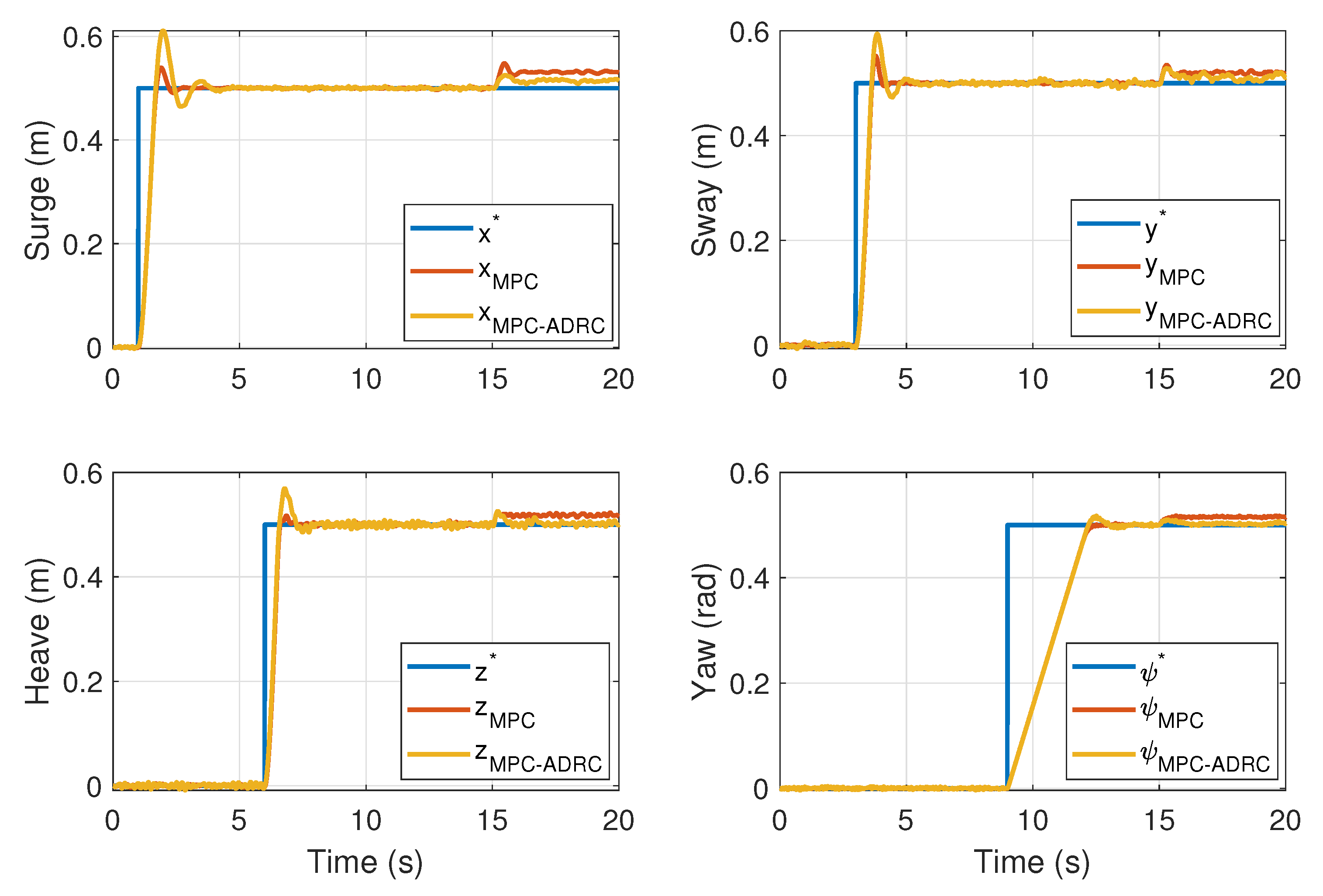
The first evaluation test compares the performance and robustness of the proposed control strategy with an MPC without the assistance of the discrete ESO. Figure 4 shows the controlled outputs of both controllers tracking predefined trajectories. This simulation also compares the capabilities of the controllers to reject external disturbances. At the time $t=15$ s, the controlled linear positions are perturbed with an external force of 1 N and the yaw angle with a moment of 1 Nm.

Both controllers, the MPC and the MPC-ADRC, have bounded control actions with $-|u_{max}|\le u\le |u_{max}|$, which allows comparing the robustness of each controller with a time integral of the square error defined as

$$ISE={\int }_{t=15}^{t=20}{\mathbf{h}}^{⊺}\left({\mathbf{x}}_r\right)\mathbf{h}\left({\mathbf{x}}_r\right)dt.$$

(46)

The $ISE$ indexes of the MPC and MPC-ADRC are shown in

Table 4. ISE index during external disturbance rejection.

MPC	MPC-ADR
0.0097	0.0024

. These results show evidence of better disturbance rejection of the MPC based on ADRC, with an $ISE$ index equivalent to 24.75% of the MPC index.

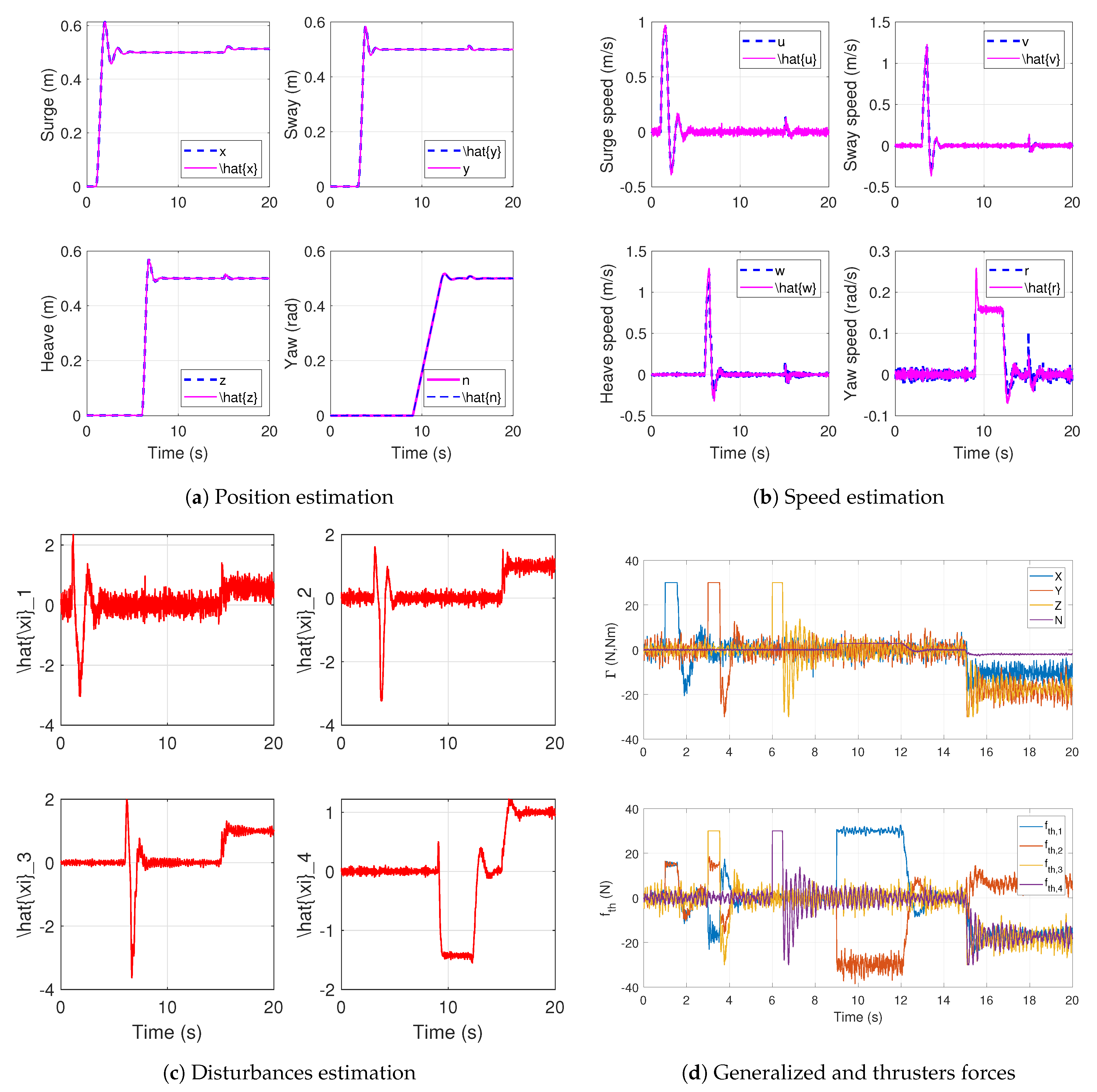
The ESO’s estimations and control signals of the MPC based on ADRC during the first evaluation are shown in Figure 5. The current position coordinates, disturbed by white noise, and their estimations are shown in Figure 5a. These position estimations result in filtered measurements, which are suitable to implement the control techniques. Figure 5b shows the current speeds and their estimations, in this figure it is shown the convergence of the estimated signals to the real speed values. Figure 5c shows the total disturbances estimation with the evolution from the estimation of model uncertainties during the first 15 seconds and the reaction to estimate the external disturbances for $t\ge 15$ s. The control signals are shown in Figure 5d, where the boundaries on the control signals are satisfied, which is evidence of satisfaction of the inequality constraints in the optimal control problem. These control signals show the controller’s reaction to reject the external disturbances in $t\ge 15$ s.

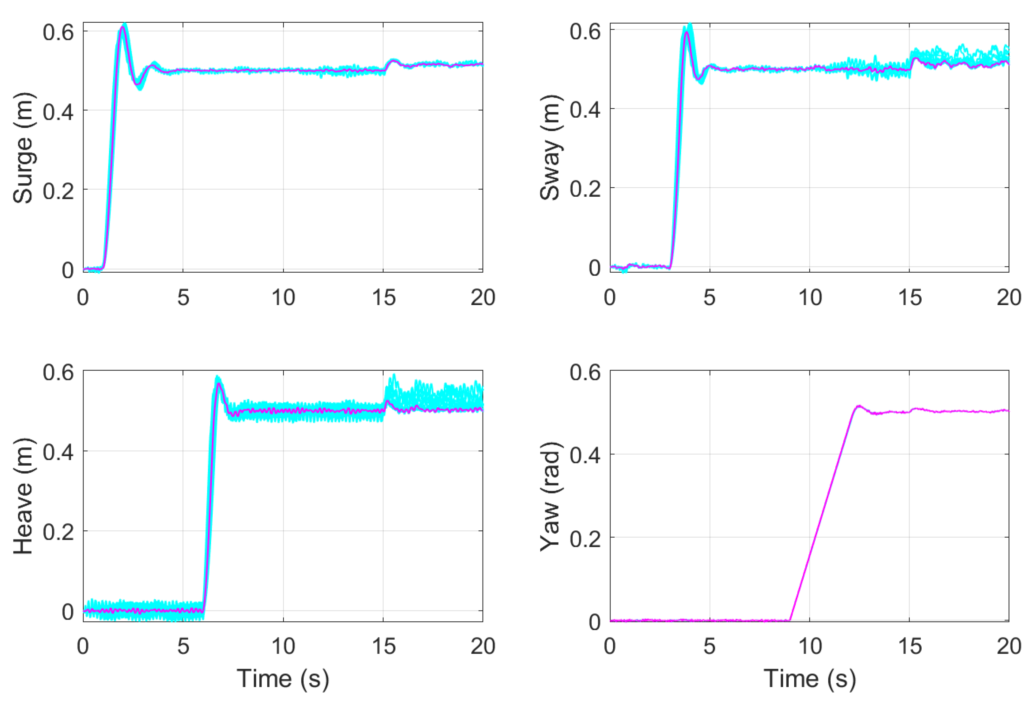
The second evaluation tests the robustness of the proposed controller against model uncertainties with simulations of parameter variations. In this evaluation, the trajectory tracking task performed during the first evaluation is repeated 21 times with values of the robot’s mass homogeneously distributed between 50% and 150% of its nominal value. Figure 6 shows the behavior of the system’s controlled output during all the simulations. The responses of the parameter variation form a cyan envelope around the nominal response in magenta, which is evidence of a bounded behavior around the nominal response and also shows robustness against model uncertainties.

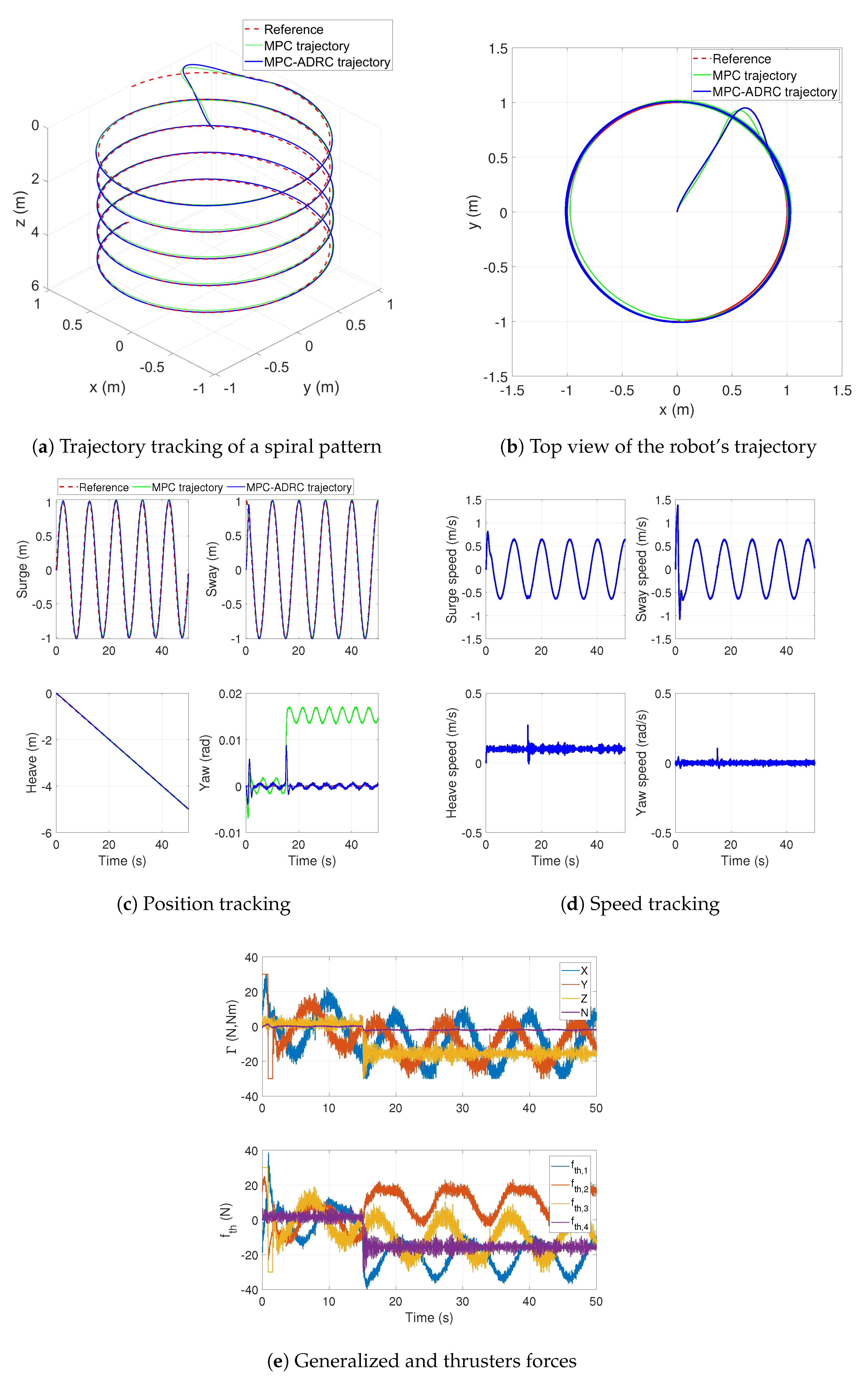
The final simulation executes a trajectory tracking task that imposes a spiral pattern starting the robot at $(0,0,0)$. The spiral reference is shown in Figure 7a, where the MPC without assistance and the MPC based on ADRC perform a transient response and then the trajectory tracking is executed. The vertical position changes at a constant speed of 0.1 m/s and goes from 0 m to 5 m. Horizontally, the robot moves in a circle centered at $(0,0)$ with a radius of 1 m. In this plane, a complete circumference is tracked every 10 s, and the robot’s position evolves according to the top view shown in Figure 7b. To test the robustness against external disturbances, an external force of 1 N is injected into the three-axis at $t=15$ s The behavior of the robot shows that both the MPC without assistance and the MPC based on ADRC accomplish tracking the trajectory; however, our control strategy achieves a better disturbance rejection, especially in the robot’s heading as shown in the yaw angle of the Figure 7c. In order to verify the satisfaction of the robot’s physical limitation during the test of the MPC based on ADRC, the robot’s velocity is shown in Figure 7d, where the maximum speed is bounded under a maximum of 1.5 m/s, which is an acceptable value for the robotic AUV. Likewise, the control signals are shown in Figure 7e, where the satisfaction of the inequality constraints of the optimal control problem is evidenced.

4. Conclusions

A robust model predictive control was developed using the active disturbance rejection control approach to estimate a total disturbance that lumps the nonlinearities, model uncertainties, and external disturbances into a unified signal. This signal is estimated using a discrete extended disturbance observer that also finds an estimation of the state vector. Then, the proposed control strategy uses the estimated disturbance and states to find an optimal control sequence for a receding horizon by using a simplified canonical model, which simplifies the dynamic constraints during the solution of the optimal control problem. The first element of the optimal control sequence and the disturbance estimation are used to define a control law, which is imposed through feedback control action that guarantees reference tracking, external disturbance rejection, and attenuation of model uncertainties.

To evaluate the proposed control strategy, a robotic autonomous underwater vehicle was used as a test platform. A protocol of three evaluation scenarios was executed in simulation to test the robustness of the proposed control. The performance of the MPC based on ADRC is compared with an MPC without the assistance of the discrete ESO. The evaluation tests show evidence of effective trajectory tracking and robustness against external disturbances and parameter uncertainties. Future work will explore the physical implementation of the proposed control strategy into an evaluation prototype of a robotic autonomous underwater vehicle.

References

1. Camacho, E.F.; Alba, C.B. Model Predictive Control; Springer Science & Business Media: Berlin/Heidelberg, Germany, 2013. [Google Scholar]
2. Qin, S.J.; Badgwell, T.A. A survey of industrial model predictive control technology. Control Eng. Pract. 2003, 11, 733–764. [Google Scholar]
3. Shen, C.; Shi, Y.; Buckham, B. Trajectory tracking control of an autonomous underwater vehicle using Lyapunov-based model predictive control. IEEE Trans. Ind. Electron. 2017, 65, 5796–5805. [Google Scholar]
4. Yan, Z.; Gong, P.; Zhang, W.; Wu, W. Model predictive control of autonomous underwater vehicles for trajectory tracking with external disturbances. Ocean Eng. 2020, 217, 107884. [Google Scholar]
5. Campo, P.J.; Morari, M. Robust model predictive control. In Proceedings of the 1987 American Control Conference, Minneapolis, MN, USA, 10–12 June 1987; pp. 1021–1026. [Google Scholar]
6. Nagy, Z.K.; Braatz, R.D. Robust nonlinear model predictive control of batch processes. AIChE J. 2003, 49, 1776–1786. [Google Scholar]
7. Allgower, F.; Findeisen, R.; Nagy, Z.K. Nonlinear model predictive control: From theory to application. J. Chin. Inst. Chem. Eng. 2004, 35, 299–316. [Google Scholar]
8. Heshmati-Alamdari, S.; Karras, G.C.; Marantos, P.; Kyriakopoulos, K.J. A robust predictive control approach for underwater robotic vehicles. IEEE Trans. Control Syst. Technol. 2019, 28, 2352–2363. [Google Scholar] [CrossRef]
9. Chen, H. A Feasible Moving Horizon H Control Scheme for Constrained Uncertain Linear Systems. IEEE Trans. Autom. Control 2007, 52, 343–348. [Google Scholar] [CrossRef]
10. Adetola, V.; DeHaan, D.; Guay, M. Adaptive model predictive control for constrained nonlinear systems. Syst. Control Lett. 2009, 58, 320–326. [Google Scholar] [CrossRef]
11. Zhang, G.; Yan, W.; Gao, J.; Liu, C. High-gain observer-based model predictive control for cross tracking of underactuated autonomous underwater vehicles. In Proceedings of the 2016 IEEE International Conference on Underwater System Technology: Theory and Applications (USYS), Penang, Malaysia, 13–14 December 2016; pp. 115–120. [Google Scholar]
12. Gao, J.; Zhang, G.; Wu, P.; Zhao, X.; Wang, T.; Yan, W. Model predictive visual servoing of fully-actuated underwater vehicles with a sliding mode disturbance observer. IEEE Access 2019, 7, 25516–25526. [Google Scholar] [CrossRef]
13. Yang, H.; Deng, F.; He, Y.; Jiao, D.; Han, Z. Robust nonlinear model predictive control for reference tracking of dynamic positioning ships based on nonlinear disturbance observer. Ocean Eng. 2020, 215, 107885. [Google Scholar] [CrossRef]
14. Vu, M.T.; Le, T.H.; Thanh, H.L.N.N.; Huynh, T.T.; Van, M.; Hoang, Q.D.; Do, T.D. Robust position control of an over-actuated underwater vehicle under model uncertainties and ocean current effects using dynamic sliding mode surface and optimal allocation control. Sensors 2021, 21, 747. [Google Scholar] [CrossRef] [PubMed]
15. Zheng, J.; Song, L.; Liu, L.; Yu, W.; Wang, Y.; Chen, C. Fixed-time sliding mode tracking control for autonomous underwater vehicles. Appl. Ocean Res. 2021, 117, 102928. [Google Scholar] [CrossRef]
16. An, S.; Wang, L.; He, Y.; Yuan, J. Adaptive Backstepping Sliding Mode Tracking Control For Autonomous Underwater Vehicles With Input Quantization. Adv. Theory Simul. 2022, 5, 2100445. [Google Scholar]
17. Zhang, Y.; Liu, J.; Yu, J. Adaptive asymptotic tracking control for autonomous underwater vehicles with non-vanishing uncertainties and input saturation. Ocean Eng. 2023, 276, 114280. [Google Scholar] [CrossRef]
18. Wang, H.D.; Zhai, Y.X.; Shah, U.H.; Karkoub, M.; Li, M. Adaptive fuzzy control of underwater vehicle manipulator system with dead-zone band input nonlinearities via fuzzy performance and disturbance observers. Ocean Eng. 2023, 277, 114194. [Google Scholar] [CrossRef]
19. Huang, F.; Xu, J.; Wu, D.; Cui, Y.; Yan, Z.; Xing, W.; Zhang, X. A general motion controller based on deep reinforcement learning for an autonomous underwater vehicle with unknown disturbances. Eng. Appl. Artif. Intell. 2023, 117, 105589. [Google Scholar] [CrossRef]
20. Lamraoui, H.C.; Qidan, Z. Path following control of fully-actuated autonomous underwater vehicle in presence of fast-varying disturbances. Appl. Ocean Res. 2019, 86, 40–46. [Google Scholar] [CrossRef]
21. Bock, H.G.; Plitt, K.J. A multiple shooting algorithm for direct solution of optimal control problems. IFAC Proc. Vol. 1984, 17, 1603–1608. [Google Scholar] [CrossRef]
22. Karras, G.C.; Marantos, P.; Bechlioulis, C.P.; Kyriakopoulos, K.J. Unsupervised online system identification for underwater robotic vehicles. IEEE J. Ocean. Eng. 2018, 44, 642–663. [Google Scholar] [CrossRef]
23. Snam, E. Nomenclature for Treating the Motion of a Submerged Body through a Fluid; Technical and Research Bulletin 1–5; The Society of Naval Architects and Marine Engineers: Jersey City, NJ, USA, 1950. [Google Scholar]
24. Fossen, T.I. Handbook of Marine Craft Hydrodynamics and Motion Control; John Wiley & Sons: Hoboken, NJ, USA, 2011. [Google Scholar]
25. Fossen, T.I. Guidance and Control of Ocean Vehicles. Ph.D. Thesis, University of Trondheim, Trondheim, Norway, 1999. [Google Scholar]
26. Arcos-Legarda, J.; Cortes-Romero, J.; Beltran-Pulido, A.; Tovar, A. Hybrid disturbance rejection control of dynamic bipedal robots. Multibody Syst. Dyn. 2019, 46, 281–306. [Google Scholar] [CrossRef]
Figure 1. Control loop for a robust MPC based on ADRC and a discrete ESO.
Jmse 11 00929 g001
Figure 2. Prediction horizon and optimal control sequence for time k.
Jmse 11 00929 g002
Figure 3. Robotic autonomous underwater vehicle.
Jmse 11 00929 g003
Figure 4. Tracking trajectory and external disturbance rejection.
Jmse 11 00929 g004
Figure 5. Extended state observer estimations and control signals.
Jmse 11 00929 g005
Figure 6. Robustness against model uncertainties. Mass variation between 50% and 150% of the nominal value.
Jmse 11 00929 g006
Figure 7. Trajectory tracking with external disturbance rejection.
Jmse 11 00929 g007