Abstract
The environmental contours represent an approach for defining extreme environmental conditions, resulting in extreme responses of marine structures with a given return period. Over the past decade, an increasing number of studies have been developed dealing with the methods for defining environmental contours and enhancing their practical application in different marine environments. In the present study, environmental contours describing significant wave heights and peak wave periods are created for the Adriatic Sea. This small semi-enclosed sea basin within the Mediterranean Sea encounters increasing maritime and offshore activities. Considering also a great but still unused potential for the installation of renewable energy facilities, the main motives for the presented study are concluded. The environmental contours are established based on 24 years of hindcast wave data extracted from the WorldWaves database. Joint distributions consisting of the marginal distribution of significant wave height and conditional distributions of peak wave periods are used as a basis for the creation of environmental contours using the IFORM and ISORM methods. Return periods of 1 year, 25 years, and 100 years are considered relevant for the marine operation, design of ships, and offshore structures, respectively. A possibility of environmental contour practical application to the calculation of global wave loads upon ship structures is presented. Based on the uncertainty assessment performed, conservative environmental contours for the whole Adriatic are also presented.
1. Introduction
Several approaches are presented in Det Norske Veritas (DNV) recommendations [1] to describe the extreme value distribution of wave conditions. Alongside design sea state and extreme individual wave height, as already well-established procedures, is the currently intensely researched environmental contour (EC) approach. It is a method applied to approximate and visually present long-term extreme sea states and responses.
Although a more precise estimation of the long-term structural responses can be obtained by integrating the product of the short-term response distribution, and the long-term joint distribution of the environmental conditions, the so-called ‘‘full long-term analysis’’ [2], the EC method is considerably less computationally demanding. Additionally, considering the ability to be incorporated within well-established structural design methodologies, compliant with instituted guidelines [1,3,4], the EC method is commonly used to get a first estimate or even as a complete replacement for a full long-term analysis.
While it can be applied for predictions over some large sea areas (e.g., ship structural analysis [5]), it is mostly used to make predictions for a specific site for coastal and offshore applications such as offshore oil and gas platforms and renewable energy structures [6]. Renewable energy applications, e.g., wave energy converters [7,8,9] or wind farms [10,11], have been extensively investigated in the literature, particularly over the past few years following global goals of decarbonization and sustainability.
Various approaches for deriving an EC from a metocean dataset have been proposed in the literature. The process generally includes the estimation of the joint distribution of the environmental variables and contour construction based on the defined joint distribution. A joint distribution can be defined by global hierarchical models [12], copula models [13], non-parametric models (for example, kernel density estimates) [11,14], or conditional extremes models [15]. Additionally, a method for the estimation of model parameters can vary between maximum likelihood estimation (MLE), method of moments (MOM), or least squares fit (LSQ), weighted or not.
The contour construction methods can be classified based on the variable space used for creation and associated exceedance probability. The EC can be created in standard normal space (inverse first-order reliability method (IFORM) [16], inverse second-order reliability method (ISORM) [17], and inverse directional simulation [15]) or directly in physical variable space (direct sampling (DS) method [18], direct IFORM [19], and highest density contour (HDC) method [20]). Based on a target exceedance probability, EC can be evaluated based on marginal exceedance probability or total exceedance probability [21].
Probably the most commonly applied approach is the inverse first-order reliability method (IFORM), proposed by Winterstein [16]. The IFORM utilizes Rosenblatt transformation on the joint distribution of environmental variables and linearizes the failure surface at the design point. Therefore, depending on the true nature of the failure surface, IFORM can underestimate the return values. Modification of the failure surface towards the second-order approximation (a circle for 2D cases) is proposed by Chai and Leira [17], suggesting the inverse second-order reliability method (ISORM). The only difference in contour creation between the two approaches, assuming an equal joint model is used, occurs within reliability index values. The ISORM yields higher values, therefore resulting in more conservative contours.
The first comprehensive overview of EC methods in general, with a special dedication to structural reliability analysis applications, is given by Ross et al. [22]. The paper describes different approaches to estimating the joint distribution of environmental variables and corresponding EC based on that distribution. The recommendation as to when and how they should be used is proposed at the end. A comparison framework for evaluating ECs of extreme sea states is developed by Eckert et al. [23]. This paper develops generalized metrics for comparing the performance of contour methods to one another among study sites. These metrics were developed to evaluate the accuracy, physical validity, and aggregated temporal performance. By applying these metrics, users can compare and select the best contour method to predict extreme sea states at a certain location for a given application. Another detailed benchmark on the robustness of EC methods and sampling uncertainty was carried out by Haselsteiner et al. [24]. The results showed significant discrepancies in both maximum significant wave height (Hs) predictions and the amount of data points occurring outside of a given contour caused by variability from different joint distribution models and different contour construction methods. The choice of joint distribution appears to have more impact.
The pioneering research of wave statistics in the Adriatic region was performed by Tabain in [25,26], developing wave histograms and specific wave spectrum (Tabain’s spectrum) as a single parameter modification of the JONSWAP spectrum relevant for the Adriatic. Tabain’s spectral and statistical description of waves was created based on the limited number of wave measurements and observations from merchant and meteorological ships. A collection of wave data from visual observation across the Adriatic [27] was later used in [28] to develop extreme wave statistics using the three-parameter Weibull distribution. However, the data from [27] suffered from uncertainties due to the lack of extremes caused by heavy weather avoidance and visual wave observation inaccuracies. Recently, the long-term, high-quality hindcast wave database, the WorldWaves Atlas (WWA), developed by Fugro Oceanor, has been used for environmental description in the Adriatic. Comparative analysis performed in [29] indicated that WWA is conservative compared to other databases available for the Adriatic. The WWA has been extensively used across different recent studies in the Adriatic, for example, the wave loads and operability analysis [30], the extreme value analysis [31], and renewable energy potential [32].
The aim of the present study is to develop ECs for the Adriatic Sea, the semi-enclosed sea basin within the Mediterranean Sea with increasing maritime and offshore activities. Two methods for environmental contours are compared, as well as different location parameters of the marginal distribution of wave heights, contributing thus to the uncertainty analysis of the long-term description of the marine environment, as the present concern of the international research community [33]. The practical application of EC is presented in the example of the short-term extreme vertical wave bending moments on oil tankers of different sizes sailing in the Adriatic. The present study is carried out for the whole Adriatic basin, representing the continuation of the research on the environmental description in the Adriatic for different types of marine applications, e.g., wave loads on damaged ships [34]. ECs presented in the paper enable engineers and decision makers a quick and reliable estimate of marine structures loading during marine operations planning and for preliminary design of ships and offshore structures in the Adriatic.
The research is presented through 5 sections and an Appendix A. After the Introduction, Section 2 is divided into two subsections. The first presents the available dataset and offers a brief description of the wave climate of the Adriatic region. The second subsection of Section 2 gives an overview of the methodology used in the computation. The results are presented in Section 3. The fourth section is reserved for a discussion, followed by corresponding conclusions, given in the last section. The environmental contours for 39 locations covering the whole Adriatic are presented in Appendix A.
2. Wave Data and Methodology
2.1. Wave Data in the Adriatic Sea
The study is performed based on 24 years of wave data extracted from the World Wave Atlas (WWA) produced by Fugro OCEANOR. The WWA is the collective name for a series of comprehensive high-resolution wind and wave climate atlases, providing statistics and data for any region worldwide. The data derived from the European Centre for Medium-Range Weather Forecasts (ECMWF) wave models are calibrated by Fugro OCEANOR [35,36,37] against satellite altimetry measurements gathered from eight different satellite missions: Geosat (1986–1989), Topex (1992–2002), Topex/Poseidon (2002–2005), Jason (2002–2008), Geosat Follow-On (2000–2008), EnviSat (2002–2010), Jason-1s (2009–2012), and Jason-2 (2008–on-going).
The available data for the Adriatic region cover a latitude–longitude grid resolution of 0.5 degrees, offering 39 accessible locations presented in Figure 1. A total of 12 wind and wave parameters are available from 1997 until 2020 at each location. Covering a 24-year period at 6 h intervals, the dataset provides a total of 33,600 records per parameter. Available data include wind speed and direction, integral spectral wave parameters (e.g., Hs, peak wave period (Tp), mean wave period), and wave direction for wind-waves and swell, considered separately and combined. The WWA model data calibrated against the satellite data represent a state-of-the-art comprehensive and systematic source of wave data as input to studies in the Adriatic region [29].
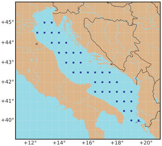
Figure 1.
The offshore grid of 39 available data points from the WWA for the Adriatic Sea.
Located in the central-north part of the Mediterranean Sea, surrounded by the Apennine in the west and Dinaric mountain ranges in the east, the Adriatic Sea stretches from the shallower northwest to the deeper southeast, with an average width of around 200 km. The surface wave creation is predominantly influenced by the northeastern wind bura and southeastern jugo. Although the strongest winds blow from the northeast, the longest fetch coincides with southeast winds yielding the highest recorded wave heights of 10.87 m.
2.2. Methodology
Statistical modeling is the first step in an EC creation carried out by constructing the joint environmental model of sea state variables of interest. The joint model used in the presented study (1), the so-called hierarchical conditional model, factorizes the joint density into the product of a marginal PDF describing the distribution of and a conditional PDF describing the .
In Equation (1), and indicate random variables, while and represent their realizations. The three-parameter Weibull distribution (2) is used for the marginal PDF of Hs where α, β, and γ represent the scale, shape, and location parameters.
The conditional PDF of Tp is modeled by a lognormal distribution as described as in (3).
The mean value and standard deviation of are conditional on Hs as follows:
The parameters of the distributions are determined by applying the maximum likelihood estimate (MLE) method on the available data for all locations.
The second part undertakes the contour construction based on the obtained joint distribution. Two chosen approaches IFORM and ISORM typically assume some type of hierarchical model as defined before. The IFORM is the most applied EC method in offshore engineering. Using the Rosenblatt transformation, the joint distribution of environmental variables is transformed to independent standard normal variables, , for the presented case:
where is the standard univariate normal CDF, while and are marginal CDF of Hs and conditional CDF of Tp, respectively. Probability of failure is then calculated in the standard normalized U-space
where denotes the PDF of standard univariate normal distribution. To solve the equation, the IFORM method assumes a linear approximation to the failure surface at the design point. The distance from the U-space origin to the design point, referred to as the reliability index ( for the IFORM), can then be calculated as (7) suggests.
The linearization of the failure surface has no a priori physical backing. Therefore, the assumption should be supported on a case-by-case basis. To overcome possible underestimation of the linearization, the ISORM approach assumes a quadratic failure surface. Instead of a tangent (hyper-)plane at the design point, Chai and Leira [17] propose a (hyper-)sphere passing through the design point and centered at the origin of the U-space. The reliability index for the ISORM approach can be calculated using (8).
where represents the inverse CDF of the chi-square distribution with n degrees of freedom, corresponding to the number of environmental variables n = 2. The failure probability is defined by a given sea state duration and return period .
A return period, also known as a recurrence interval, is frequently used to determine extreme events. In the case of marine structures, it is an average time or an estimated average time between the occurrences of the extreme sea states, i.e., extreme responses. The theoretical return period between occurrences is the inverse of the average frequency of occurrence. Ships are designed considering a return period of 25 years, which raises to 100 for offshore structures. Based on the reliability index for the prescribed return period, the circle is established in U-space.
Finally, the EC is obtained by transforming the circle from the U-space into a contour in the environmental parameter space using the inverse Rosenblatt transformation (11).
The ECs are produced for two return periods of 25 and 100 years, applying both the IFORM and ISORM approach through a Python script generated by combining several well-defined libraries, virocon [38,39] and MHKiT [40]. Results are displayed and compared for representative locations in the Adriatic.
To determine maximum responses corresponding with the ECs, the contours of the most probable extreme VWBM at midship in short-term conditions are produced relative to the value of VWBM required by the International Association of Classification Societies (IACS) Rules [41]. Transfer functions of VWBM at midship are calculated using the semi-analytical approach proposed and validated by Jensen and Mansour [42], which is particularly useful in conceptual studies such as the present one. The approach approximates a ship hull by a pontoon of equal length, equivalent breadth, and draught, while speed and block coefficient are accounted for through correction factors. The response spectrum of VWBM is computed as a product of a wave spectrum and a square modulus of a transfer function. The most probable extreme amplitude of the VWBM () is calculated by the following expression:
where is the response variance, obtained as the zeroth spectral moment, and is the number of response cycles occurring through a sea state duration.
The response analysis is performed on four classes of oil tankers, Panamax, Aframax, Suezmax, and VLCC, representing the actual size range of oil tankers operating worldwide. The average dimensions of a typical ship, i.e., a class representative presented in Table 1, are provided in [43]. A reduced ship speed of 5 knots is recommended for the evaluation of the design wave loads for strength assessment [44].

Table 1.
Main dimensions of four representative oil tankers representing the range of actual sizes.
Therefore, in the present study, ships sailing in head waves with a low forward speed of 5 knots are considered. Consistently with sea state resolution in the WWA database, 6 h is selected as the short-term sea state duration. The results of the analysis are presented in the following section together with the EC.
3. Results
Joint hierarchical models are fitted to data for all 39 locations as a base for contour creation. The 25- and 100-year contours have been created applying both IFORM and ISORM approaches. Three locations from the Adriatic sub-basins exhibiting above-average HS estimates are chosen as representative of the south (41.5° N 18.5° E), central (43.0° N 14.5° E), and north (44.5° N 13.0° E) Adriatic. A comparison of contour creation methods is displayed in Figure 2a. A 100-year contour is distinguished with a dashed line, while a full line signifies a 25-year return period. Orange and gray differentiate the IFORM and ISORM approaches, respectively, while blue circles represent hindcast wave data. The goodness of fit of marginal Weibull PDF of Hs is presented on the left, Figure 2b. Except for small deviations at the highest quantiles, a rather good fit is obtained. For central and north location Q-Q plots in Figure 2b, fitted marginal distributions of Hs seem to slightly underestimate the highest value, while for the southern part, the contrary happens. As expected, ISORM displays more conservative results yielding the largest variations at the marginal values, i.e., peaks of Hs and Tp. At the extremes, ISORM predicts around 20% higher Hs. Out of 23 years of datapoints, most fall inside the 25-year IFORM contour. However, a slight underestimation of IFORM is evident due to some high Hs data left outside the contour. Therefore, the ISORM contour is used in further response analysis and presentation.
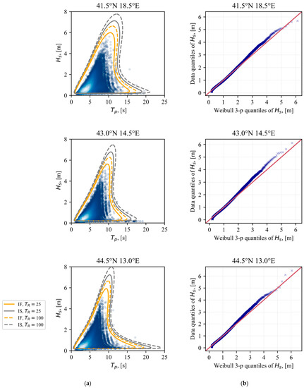
Figure 2.
A comparison of EC for three characteristic locations: (a) The comparison of IFORM and ISORM corresponding 25-year and 100-year contours; (b) Q–Q plot comparing Hs data to the corresponding fitted Weibull distribution.
The results combining ISORM EC and contours of VWBM ratio are presented in Figure 3 and Figure 4. The contours represent the percentage of the most probable extreme VWBM compared to the linear IACS Rule VWBM. The ECs reach the highest extreme VWBM ratio of almost 60% for the Panamax tanker at the southern location (upper left graph in Figure 3). At the same location, the relative VWBM for Aframax ship is slightly lower. Expectedly, with increasing the size of the oil tanker, the VWBM contours shift to the right side of the graph, i.e., towards the higher Tp, reducing VWBM relative to the IACS value. It is interesting to notice that the periods of sea states in the North Adriatic are lower, reducing relative VWBM.
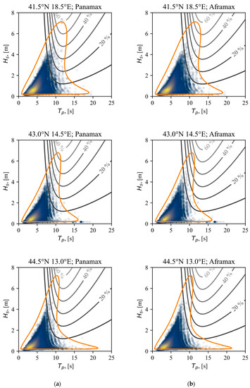
Figure 3.
The ISORM 25-year contour (orange) in comparison to VWBM contours (gray) of oil tankers for three characteristic locations: (a) Panamax contours; (b) Aframax contours.
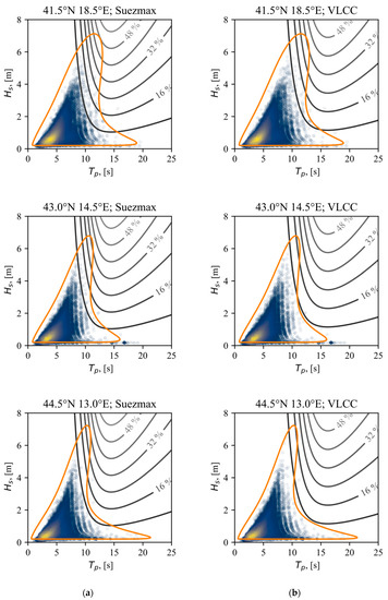
Figure 4.
The ISORM 25-year contour (orange) in comparison to VWBM contours (gray) of oil tankers for three characteristic locations: (a) Suezmax contours; (b) VLCC contours.
4. Discussion
The shape of environmental contours in the Adriatic is similar in all three locations, although in the southern part of the Adriatic (upper row in Figure 3, 41.5° N), it may be noticed that the region encompassed by EC corresponding to the highest significant wave heights is wider compared to the other locations. This indicates that the response of marine structures should be investigated for the range of wave periods, while in the central and north Adriatic, the peak wave period corresponding to the extreme wave height is almost unique. Additionally, depending on the ship type, the maximum response does not always occur for a single maximum Hs but rather for the range of Hs–Tp pairs, thus suggesting the use and implementation of ECs in extreme long-term response analysis.
In all cases, there is an “elongated tail” of EC at low significant wave heights, extended toward large wave periods. Particularly long waves of a small height and long period could be ignored as their influence on the response of marine structures is negligible.
Although the current study has not explored other contour methods and joint models, generated contours seem to describe data well. There is a slight underestimation from IFORM, whereas overestimation of the ISORM contour on the other end may be noticed. The conservative trends of the ISORM approach are supported by a plain overview of the presented Equations (7) and (8) for reliability index calculations. There are also in line with the results and conclusions published in the literature [17]. However, the ECs are sensitive to the initial joint probability distribution. The location parameter γ is the most uncertain when fitting the Weibull 3P distribution. Namely, the physical interpretation of this parameter is the minimum significant wave height representing permanent sea activity. A comparison of IFORM and ISORM ECs for various choices of γ is shown in Figure 5, where large uncertainty may be observed. The reason for these discrepancies s in the fitting of the tail of the marginal distribution of HS, which may be seen in the Q-Q plots presented in Figure 6. One can conclude from Figure 5 and Figure 6 that the Weibull 2P (Weibull 3P with location parameter equal to zero, γ = 0) distribution is completely inappropriate as the long-term distributions of HS lead to unconservative ECs.
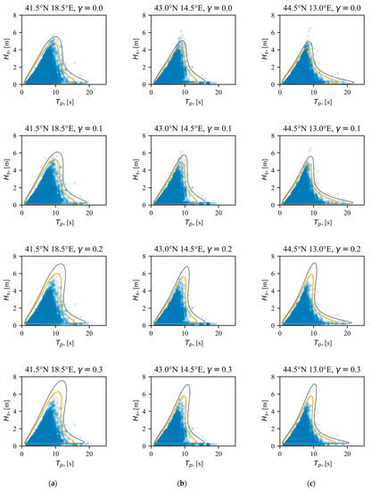
Figure 5.
The 25-year IFORM (orange) and ISORM (gray) contour based on a different variation of joint model parameters, i.e., varying location parameter γ for locations: (a) south (41.5° N 18.5° E), (b) central (43.0° N 14.5° E), and (c) north (44.5° N 13.0° E) Adriatic.
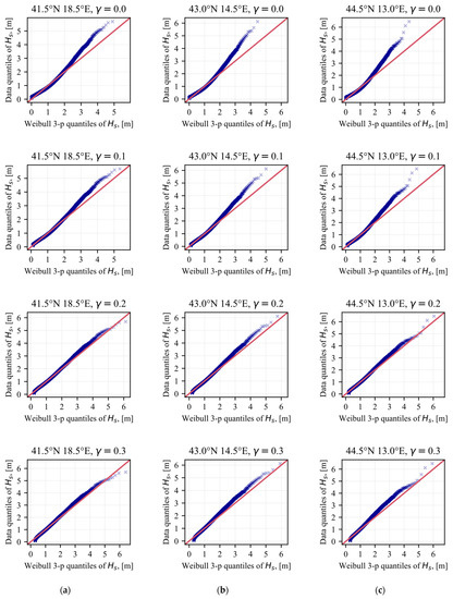
Figure 6.
The Q–Q plots illustrate a comparison of Hs data to the corresponding fitted Weibull distribution. Influence of location parameter variation γ on joint model fit for locations: (a) south (41.5° N 18.5° E), (b) central (43.0° N 14.5° E), and (c) north (44.5° N 13.0° E) Adriatic.
As the Adriatic is a semi-enclosed sea basin with rather low extreme significant wave heights, the extreme VWBM of oil tankers is not approaching the IACS Rule VWBM. Namely, Rule VWBM is intended for ocean-going ships with unrestricted service. Nevertheless, for smaller ships (Panamax tankers, in the present case), extreme VWBM in short-term sea conditions could reach 60% of the IACS Rule value. This ratio is decreased with increasing ship size. There is also a slightly larger extreme VWBM in the southern part of the Adriatic compared to other locations, although the difference between locations is generally not significant.
5. Conclusions
The development of environmental contours (ECs) for the semi-enclosed basin of the Adriatic Sea is presented in the paper. The ECs are obtained based on the joint probability distribution of significant wave heights and peak wave periods using data contained in the WorldWaves database. The joint probability distribution used in the study consisted of the Weibull 3P marginal distribution of Hs and the log-normal conditional distribution of TP.
By comparing ECs obtained using IFORM and ISORM methods, it was found that the latter leads to the conservative estimate of extreme sea states for the same choice of the joint probability distribution parameters. It is also found that ECs are highly sensitive to the joint probability model, especially to the selection of the location parameter γ of Weibull 3P distribution.
The application of ECs is shown through the example of extreme short-term vertical wave bending moments on oil tankers of different sizes, where ECs can be used to identify wave conditions leading to the largest extreme values. Although global wave loads on ships in the Adriatic are generally not approaching IACS Rule values, the benefit of using ECs is clearly shown, as they include not only extreme HS but also a range of wave steepness that may influence ship global wave-induced response.
As a result of the study, ECs for all 39 locations in the Adriatic are presented in Appendix A for three characteristic return periods of 1, 25, and 100 years. The 1-year ECs are used for planning marine operations in the Adriatic, e.g., transportation of heavy cargoes or installation of offshore platforms, while those for return periods of 25 and 100 years are useful for the design of ships and offshore structures, respectively. Although more detailed information for specific locations is required for commercial purposes, presented contours may be used for preliminary identification of extreme sea states.
Author Contributions
Conceptualization, A.M. and J.P.; methodology, A.M. and J.P.; software, A.M.; validation A.M.; formal analysis, A.M.; investigation, A.M.; resources, A.M.; data curation A.M.; writing—original draft preparation, A.M.; writing—review and editing, A.M. and J.P.; visualization, A.M.; supervision, J.P.; project administration, J.P.; funding acquisition, J.P. All authors have read and agreed to the published version of the manuscript.
Funding
This work has been fully supported by Croatian Science Foundation under the project lP-2019-04-2085.
Institutional Review Board Statement
Not applicable.
Informed Consent Statement
Not applicable.
Data Availability Statement
Not applicable.
Acknowledgments
This work has been fully supported by the Croatian Science Foundation under the project lP-2019-04-2085. The WorldWaves data are provided by Fugro OCEANOR AS.
Conflicts of Interest
The authors declare no conflict of interest. The funders had no role in the design of the study; in the collection, analyses, or interpretation of data; in the writing of the manuscript; or in the decision to publish the results.
Appendix A
The ECs based on the ISORM for all 39 locations in the Adriatic are presented in following figures for characteristic return periods of 1, 25, and 100 years.

Figure A1.
The ISORM ECs for characteristic return periods of 1, 25, and 100 years, pt.1.

Figure A2.
The ISORM ECs for characteristic return periods of 1, 25, and 100 years, pt.2.

Figure A3.
The ISORM ECs for characteristic return periods of 1, 25, and 100 years, pt.3.

Figure A4.
The ISORM ECs for characteristic return periods of 1, 25, and 100 years, pt.4.
References
- Det Norske Veritas. Recommended Practice DNV-RP-C205: Environmental Conditions and Environmental Loads; Det Norske Veritas: Oslo, Norway, 2019. [Google Scholar]
- Guedes Soares, C. Long Term Distribution of Non-Linear Wave Induced Vertical Bending Moments. Mar. Struct. 1993, 6, 475–483. [Google Scholar] [CrossRef]
- ISO 19901-1:2015; Petroleum and Natural Gas Industries, Specific Requirements for Offshore Structures: Part 1: Metocean Design and Operating Considerations. International Organization for Standardization: Geneva, Switzerland, 2005.
- NORSOK Standard N-003; Edition 3Actions and Action Effects. Norwegian Technology Standards Institution: Oslo, Norway, 2017.
- Baarholm, G.; Moan, T. Application of Contour Line Method to Estimate Extreme Ship Hull Loads Considering Operational Restrictions. J. Ship Res. 2001, 45, 228–240. [Google Scholar] [CrossRef]
- Wrang, L.; Katsidoniotaki, E.; Nilsson, E.; Rutgersson, A.; Rydén, J.; Göteman, M. Comparative Analysis of Environmental Contour Approaches to Estimating Extreme Waves for Offshore Installations for the Baltic Sea and the North Sea. J. Mar. Sci. Eng. 2021, 9, 96. [Google Scholar] [CrossRef]
- Harnois, V.; Thies, P.R.; Johanning, L. On Peak Mooring Loads and the Influence of Environmental Conditions for Marine Energy Converters. J. Mar. Sci. Eng. 2016, 4, 29. [Google Scholar] [CrossRef]
- Neary, V.S.; Ahn, S.; Seng, B.E.; Allahdadi, M.N.; Wang, T.; Yang, Z.; He, R. Characterization of Extreme Wave Conditions for Wave Energy Converter Design and Project Risk Assessment. J. Mar. Sci. Eng. 2020, 8, 289. [Google Scholar] [CrossRef]
- Katsidoniotaki, E.; Nilsson, E.; Rutgersson, A.; Engström, J.; Göteman, M. Response of Point-Absorbing Wave Energy Conversion System in 50-Years Return Period Extreme Focused Waves. J. Mar. Sci. Eng. 2021, 9, 345. [Google Scholar] [CrossRef]
- Vanem, E.; Hafver, A.; Nalvarte, G. Environmental Contours for Circular-Linear Variables Based on the Direct Sampling Method. Wind Energy 2020, 23, 563–574. [Google Scholar] [CrossRef]
- Haselsteiner, A.; Ohlendorf, J.-H.; Thoben, K.-D. Environmental Contours Based on Kernel Density Estimation. arXiv 2017. [Google Scholar] [CrossRef]
- Bitner-Gregersen, E.M. Joint Met-Ocean Description for Design and Operations of Marine Structures. Appl. Ocean Res. 2015, 51, 279–292. [Google Scholar] [CrossRef]
- Montes-Iturrizaga, R.; Heredia-Zavoni, E. Environmental Contours Using Copulas. Appl. Ocean Res. 2015, 52, 125–139. [Google Scholar] [CrossRef]
- Eckert-Gallup, A.; Martin, N. Kernel Density Estimation (KDE) with Adaptive Bandwidth Selection for Environmental Contours of Extreme Sea States. In Proceedings of the OCEANS 2016 MTS/IEEE, Monterey, CA, USA, 19–23 September 2016; pp. 1–5. [Google Scholar]
- Jonathan, P.; Ewans, K.; Randell, D. Non-Stationary Conditional Extremes of Northern North Sea Storm Characteristics. Environmetrics 2014, 25, 172–188. [Google Scholar] [CrossRef]
- Hirdaris, S.E.; Bai, W.; Dessi, D.; Ergin, A.; Gu, X.; Hermundstad, O.A.; Huijsmans, R.; Iijima, K.; Nielsen, U.D.; Parunov, J.; et al. Loads for Use in the Design of Ships and Offshore Structures. Ocean Eng. 2014, 78, 131–174. [Google Scholar] [CrossRef]
- Chai, W.; Leira, B.J. Environmental Contours Based on Inverse SORM. Mar. Struct. 2018, 60, 34–51. [Google Scholar] [CrossRef]
- Bang Huseby, A.; Vanem, E.; Natvig, B. A New Approach to Environmental Contours for Ocean Engineering Applications Based on Direct Monte Carlo Simulations. Ocean Eng. 2013, 60, 124–135. [Google Scholar] [CrossRef]
- Derbanne, Q.; de Hauteclocque, G. A New Approach for Environmental Contour and Multivariate De-Clustering. In Proceedings of the ASME 2019 38th International Conference on Ocean, Offshore and Arctic Engineering, Glasgow, UK, 9–14 June 2019; Volume 3. [Google Scholar]
- Haselsteiner, A.F.; Ohlendorf, J.-H.H.; Wosniok, W.; Thoben, K.-D.D. Deriving Environmental Contours from Highest Density Regions. Coast. Eng. 2017, 123, 42–51. [Google Scholar] [CrossRef]
- Mackay, E.; Haselsteiner, A.F. Marginal and Total Exceedance Probabilities of Environmental Contours. Mar. Struct. 2021, 75, 102863. [Google Scholar] [CrossRef]
- Ross, E.; Astrup, O.C.; Bitner-Gregersen, E.; Bunn, N.; Feld, G.; Gouldby, B.; Huseby, A.; Liu, Y.; Randell, D.; Vanem, E.; et al. On Environmental Contours for Marine and Coastal Design. Ocean Eng. 2020, 195, 106194. [Google Scholar] [CrossRef]
- Eckert, A.; Martin, N.; Coe, R.G.; Seng, B.; Stuart, Z.; Morrell, Z. Development of a Comparison Framework for Evaluating Environmental Contours of Extreme Sea States. J. Mar. Sci. Eng. 2021, 9, 16. [Google Scholar] [CrossRef]
- Haselsteiner, A.F.; Coe, R.G.; Manuel, L.; Chai, W.; Leira, B.; Clarindo, G.; Guedes Soares, C.; Hannesdóttir, Á.; Dimitrov, N.; Sander, A.; et al. A Benchmarking Exercise for Environmental Contours. Ocean Eng. 2021, 236, 109504. [Google Scholar] [CrossRef]
- Tabain, T. The Proposal for the Standard of Sea States for the Adriatic. Brodogradnja 1974, 25, 251–258. [Google Scholar]
- Tabain, T. Standard Wind Wave Spectrum for the Adriatic Sea Revisited (1977–1997). Brodogradnja 1997, 45, 303–313. [Google Scholar]
- Hydrographic Institute of Republic of Croatia. Atlas of the Climatology of the Adriatic Sea; HHI: Split, Croatia, 1979. (In Croatian) [Google Scholar]
- Parunov, J.; Ćorak, M.; Pensa, M. Wave Height Statistics for Seakeeping Assessment of Ships in the Adriatic Sea. Ocean Eng. 2011, 38, 1323–1330. [Google Scholar] [CrossRef]
- Ćorak, M.; Mikulić, A.; Katalinić, M.; Parunov, J. Uncertainties of Wave Data Collected from Different Sources in the Adriatic Sea and Consequences on the Design of Marine Structures. Ocean Eng. 2022, 266, 112738. [Google Scholar] [CrossRef]
- Petranović, T.; Mikulić, A.; Katalinić, M.; Ćorak, M.; Parunov, J. Method for Prediction of Extreme Wave Loads Based on Ship Operability Analysis Using Hindcast Wave Database. J. Mar. Sci. Eng. 2021, 9, 1002. [Google Scholar] [CrossRef]
- Katalinić, M.; Parunov, J. Comprehensive Wind and Wave Statistics and Extreme Values for Design and Analysis of Marine Structures in the Adriatic Sea. J. Mar. Sci. Eng. 2021, 9, 522. [Google Scholar] [CrossRef]
- Farkas, A.; Degiuli, N.; Martić, I. Assessment of Offshore Wave Energy Potential in the Croatian Part of the Adriatic Sea and Comparison with Wind Energy Potential. Energies 2019, 12, 2357. [Google Scholar] [CrossRef]
- Bitner-Gregersen, E.M.; Waseda, T.; Parunov, J.; Yim, S.; Hirdaris, S.; Ma, N.; Guedes Soares, C. Uncertainties in Long-Term Wave Modelling. Mar. Struct. 2022, 84, 103217. [Google Scholar] [CrossRef]
- Parunov, J.; Rudan, S.; Ćorak, M. Ultimate Hull-Girder-Strength-Based Reliability of a Double-Hull Oil Tanker after Collision in the Adriatic Sea. Ships Offshore Struct. 2017, 12, S55–S67. [Google Scholar] [CrossRef]
- Barstow, S.; Mørk, G.; Lønseth, L.; Schjølberg, P.; Machado, U.; Athanassoulis, G.; Belibassakis, K.A.; Gerostathis, T.; Stefanakos, C.; Spaan, G. WORLDWAVES: Fusion of Data from Many Sources in a User-Friendly Software Package for Timely Calculation of Wave Statistics in Global Coastal Waters. In Proceedings of the 13th International Offshore and Polar Conference and Exhibition, ISOPE2003, Honolulu, HI, USA, 25–30 May 2003; pp. 136–143. [Google Scholar]
- Barstow, S.; Mørk, G.; Lønseth, L.; Schjølberg, P.; Machado, U.; Athanassoulis, G.; Belibassakis, K.A.; Gerostathis, T.; Stefanakos, C.; Spaan, G. WORLDWAVES: High Quality Coastal and Offshore Wave Data within Minutes for Any Global Site. In Proceedings of the OMAE03 22nd International Conference on Offshore Mechanics and Arctic Engineering, Cancun, Mexico, 8–13 June 2003. [Google Scholar]
- Barstow, S.; Mørk, G.; Lønseth, L.; Mathisen, J. WorldWaves Wave Energy Resource Assessments from the Deep Ocean to the Coast. J. Energy Power Eng. 2011, 5, 730–742. [Google Scholar]
- Haselsteiner, A.F.; Lehmkuhl, J.; Pape, T.; Windmeier, K.-L.; Thoben, K.-D. ViroCon: A Software to Compute Multivariate Extremes Using the Environmental Contour Method. SoftwareX 2019, 9, 95–101. [Google Scholar] [CrossRef]
- Haselsteiner, A.F.; Windmeier, K.-L.; Ströer, L.; Thoben, K.-D. Update 2.0 to “ViroCon: A Software to Compute Multivariate Extremes Using the Environmental Contour Method”. SoftwareX 2022, 20, 101243. [Google Scholar] [CrossRef]
- Klise, K.; Pauly, R.; Ruehl, K.M.; Olson, S.; Shippert, T.; Morrell, Z.; Bredin, S.; Lansing, C.; Macduff, M.; Martin, T.; et al. MHKiT (Marine and Hydrokinetic Toolkit)—Python [Computer Software]. 2020. Available online: https://github.com/MHKiT-Software/MHKiT-Python (accessed on 18 April 2023).
- IACS. IACS International Association of Classicfication Societies; IACS: London, UK, 2019; pp. 1–13. [Google Scholar]
- Jensen, J.J.; Mansour, A.E. Estimation of Ship Long-Term Wave-Induced Bending Moment Using Closed-Form Expressions. RINA Trans. 2002, 144, 41–55. [Google Scholar]
- Michel, R.K.; Osborne, M. Oil Tankers. In Ship Design and Construction; Lamb, T., Ed.; SNAME: Jersey City, NJ, USA, 2004; pp. 29.1–29.41. [Google Scholar]
- IACS. Rec. No. 34. Rev.2 Standard Wave Data (North Atlantic Scatter Diagramm); IACS: London, UK, 2022. [Google Scholar]
Disclaimer/Publisher’s Note: The statements, opinions and data contained in all publications are solely those of the individual author(s) and contributor(s) and not of MDPI and/or the editor(s). MDPI and/or the editor(s) disclaim responsibility for any injury to people or property resulting from any ideas, methods, instructions or products referred to in the content. |
© 2023 by the authors. Licensee MDPI, Basel, Switzerland. This article is an open access article distributed under the terms and conditions of the Creative Commons Attribution (CC BY) license (https://creativecommons.org/licenses/by/4.0/).