Abstract
The recognition of submarine cable magnetic anomaly (SCMA) signals is a challenging task in magnetic signal data processing. In this study, a multi-task convolutional neural network (MTCNN) model is proposed to simultaneously recognize abnormal signals and locate abnormal regions. The residual block is added to the shared feature backbone to improve the ability of the network to extract high-level features and maintain the gradient stability of the model in the training process. The long short-term memory (LSTM) block is added to the classification branch task to learn the internal relationship of the magnetic anomaly time series, so as to improve the network’s ability to recognize magnetic anomalies. Our proposed model can accurately recognize the SCMA signals collected in the East China Sea and the South China Sea. The classification accuracy and the ability to locate the abnormal regions are close to the manual labeling of human analysts. The newly developed model can help analysts reduce the probability of missing and misjudging submarine cable magnetic anomalies, improve the efficiency and accuracy of interpretation, and could even be deployed to an unmanned platform to realize the automatic detection of SCMAs.
1. Introduction
At present, the recognition of SCMA signals mainly relies on manual methods [1,2,3]. The main challenges of manual methods are the lack of real-time processing options, heavy processing workload and slow processing speed. Furthermore, in the face of a large amount of data to be analyzed and processed, analysts may misjudge or miss abnormal magnetic signals.
The recognition target simplified as a magnetic dipole model has been studied more. The Frumkis team proposed the standard orthogonal basis function (OBF) detection theory for magnetic anomaly target recognition for the first time, constructed the energy function of the magnetic anomaly signals using the OBF, verified the performance of the detection method using the simplified model [4,5], and subsequently optimized the parameters such as sliding window and offset to further improve its detection performance [6]. Under the condition of Gaussian white noise, the OBF detector has the best detection performance, but in the presence of non-Gaussian white noise, the detection performance is greatly affected. In view of the dependence of OBF detector on environmental noise, researchers have successively proposed whitening filtering [7,8,9] and wavelet decomposition [10,11] methods to suppress the environmental noise, further improving the practicability of the OBF detection method. The dependence of OBF detector on Gaussian white noise greatly limits its performance, so other detection methods based on target characteristic signals have also been studied, such as stochastic resonance [12] and principal component analysis [13] methods. At present, most of the magnetic anomaly target recognition methods are based on the signal detection theory. By converting the signal point by point to the feature domain, the decision statistics are generated, then the existence of magnetic anomaly target signals is judged by comparing with the threshold value. However, first of all, magnetic anomaly target detection can actually be regarded as a pattern recognition process, and its feature extraction scheme should not be limited to the framework of signal detection. Secondly, the signal of the magnetic anomaly target is different from the background in the form of data segments. Judging the existence of the target point by point is contrary to people’s intuitive cognition of the existence of magnetic anomaly targets. Finally, the magnetic anomaly characteristics of submarine cable are different from the magnetic dipole signals, so the existing methods based on signal detection theory are not suitable for the recognition of SCMAs.
Machine learning methods provide a key solution for this. From the view of signal sample representation, the detection of magnetic anomaly target signals in data segments is conducive to avoiding the impact of point anomalies and further improving the recognition accuracy. Zhao and Zhang used the neural network method to classify and extract segmented magnetic anomaly target signals, effectively improving the detection performance of magnetic anomaly targets [14,15,16]. All the above methods transform one-dimensional magnetic signals into time-frequency signals and then identify magnetic anomalies, but the time-frequency analysis process greatly reduces the efficiency from original data to recognition.
Therefore, this study developed an end-to-end multi-task learning network for total magnetic field anomalies recognition of submarine power cables. We first used a one-dimensional residual convolutional network for feature extractions of magnetic anomaly signals, and then in a second stage performed a classification branch task to identify the anomaly and executed regression branch tasks to pick the minimum and maximum position of magnetic anomalies. Recurrent neural networks are designed for processing the high-level features from the magnetic signal time sequence. They can learn the internal temporal relations and share features learned from the different positions in the time series. A residual learning framework is employed in this study to make deeper learning feasible, which allows extraction of higher-level features and building more complex networks. Field data are tested to demonstrate the performance of the networks. The network model proposed in this study can solve the problems of traditional manual methods in recognizing SCMAs, achieve automatic recognition of SCMAs, and improve the efficiency and accuracy of recognizing SCMAs.
2. Methods
2.1. Network Design
Total magnetic field signals gathered by the boat towing for continuous measurement are time series consisting of local characteristics (SCMAs) and global characteristics (background geomagnetic fields). Therefore, multiple convolutional layers are first added to the networks to extract the local and global characteristics (Figure 1). Traditionally, recurrent neural networks have been used for sequence modeling. Here, we use the long short-term memory (LSTM) [17] block to reduce the dimension of the extracted time series features and remember its internal relationship (Figure 1).
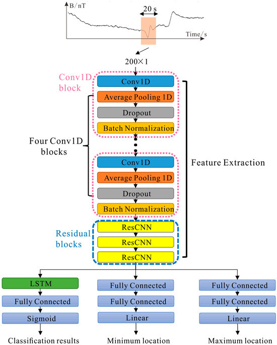
Figure 1.
The multi-task learning networks architecture for magnetic anomaly recognition. The input sample data are magnetic data with a length of 20 s. The data sampling rate is 0.1 s, so the input sample length is 200 sampling points. The shared feature extraction backbone network includes four one-dimensional convolutional blocks and three residual blocks. The one-dimensional convolutional block consists of a one-dimensional convolutional layer, average pooling layer, dropout layer and batch normalization layer.
A multi-task network of recurrent and convolutional layers is built to perform SCMA recognition (Figure 1). The overall architecture of our networks includes shared feature extraction backbone network and three separate, fully connected branch networks. A fully connected network with a LSTM block is used to judge the existence of SCMA signals. The other two fully connected branch networks determine the minimum and maximum location of magnetic anomaly signals (Figure 1).
2.2. Sequential Learning
The LSTM layer performs sequential learning to reduce the vanishing/exploding gradient problem. A LSTM unit has an internal memory cell, which contains three gates, namely the forget, update and output gates (Figure 2). The forget gate learns how much information is to be retained or forgotten from the memory block. The update gate learns what information is to be stored in the memory block. The output gate determines what information can be used for the output [17]. The LSTM unit calculation process is as follows:
where is the candidate value for replacing the memory, is a forget gate, is an update gate and is an output gate. is the nonlinear function of the input weighted sum at time t. is the state of previous time step. The Ws and bs are weights and bias terms. The is the Sigmoid activation functions:
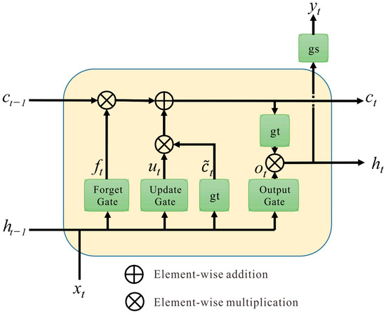
Figure 2.
A LSTM unit which has the long-term memory h, and the short-term memory c.
The memory cell value at each time step will be calculated using the candidate value at current step and previous value .
where is element-wise multiplication. The final state is calculated with the output gate value and the memory cell value :
where is the Tanh activation function:
The final predicted output at time :
2.3. Residual Learning
Increasing the depth of neural networks will also increase the training difficulty, which may lead to the vanishing or exploding gradients and affect the convergence of the model. In order to avoid the above problems, the residual learning [18] method is introduced. Through this framework, higher-level magnetic signal features can be extracted to ensure that the network’s deep learning ability does not degenerate.
Two stacked one-dimensional convolutional layers in every residual learning block. Each one-dimensional convolutional layer is followed by one batch normalization layer (Figure 3). The building block is defined as:
where and are the input and output vectors of the block. The function is the residual mapping to be learned. where represents ReLU [19] and biases are omitted to simplify representation. A linear projection is performed by the shortcut connections to match the dimensions. is performed by element-wise addition. The second ReLU is added after addition.
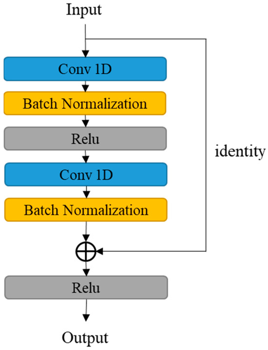
Figure 3.
A residual learning block that is the ResCNN block in Figure 1.
2.4. Non Maximum Suppression
Non-maximum suppression [20] is widely used in deep learning target detection algorithms, such as YOLO [21] and Faster-RCNN [22] etc., where the optimal solution can be obtained by screening out the local maximum value. Inspired by this, the non-maximum suppression method is used to select the optimal abnormal target region for the detection of SCMA signals. The specific algorithm is implemented as follows:
Step 1: multiple different prediction regions and their corresponding confidence levels can be obtained after inputting magnetic signal sequence into the model. A set H containing the predicted candidate regions is constructed and initialized to contain all regions. Build a set M holding the optimal region and initialize it as the empty set.
Step 2: all regions in set H are sorted, and the region S with the highest confidence score is selected to move from set H to set M.
Step 3: each region in set H is calculated as an interaction-over-union (IoU) with region S. If it is higher than a certain threshold (generally 0~0.5), this region is considered to overlap with region S, and this region is removed from set H.
Step 4: go back to step 2 and iterate until the set H is empty. The region in set M is the predicted location of the magnetic anomalies.
Suppose that one prediction region is A and the other is B, as shown in Figure 4, then the calculation formula of IoU is as follows:
where IoU represents the proportion of the length of intersection of regions A and B to the length of union of regions A and B.

Figure 4.
Calculation diagram of IoU between prediction regions A and B.
3. Results
3.1. Network Architecture
The new proposed network architecture MTCNN is shown in Figure 1. The network is divided into two parts, shared feature extraction and anomaly detection. The readers refer to Table 1 for details.

Table 1.
The parameters of the MTCNN model.
The input into the network is the raw magnetic signal with 200 sampling points. The model assumes that the range of 200 sampling points can include all kinds of SCMAs. Among the shared feature extraction part, we use four one-dimensional convolutional blocks to get the high-level features. Each convolutional block consists of a one-dimensional convolutional layer with a rectified linear unit (Relu) activation function, an average pooling layer, a batch normalization layer, and a dropout layer. Batch normalization layers normalize the activation output of the convolutional layer (Figure 1), which can prevent overfitting and accelerate the training [23]. In order to further extract higher-level features, residual blocks [18] are added in the network, which makes it possible to train a deeper network without degradation.
After shared feature extraction backbone, three branch tasks are added—one branch for detecting the existence of a SCMA signal and the other two branches for regressing the minimum and maximum locations of a SCMA signal (Figure 1).
For the branch discriminating the existence of a SCMA signal, one LSTM layer is added after feature extraction (Figure 1). A combination of recurrent and convolutional layers has been proven to be an effective architecture for sequential modeling [24,25,26]. LSTM layer can learn the internal temporal relations and share features learned from the different positions in the sequence. Two fully connected layers are placed behind the LSTM layer, carrying out advanced reasoning and map the sequence model to the desired output classes. A Sigmoid binary activation is used in the last fully connected layer. The output is the predicted probability of each sample of magnetic signals.
For the other two branches regressing the minimum and maximum locations of a SCMA signal, three fully connected layers in each branch task are added behind feature extraction (Figure 1). Linear activation is used in the last fully connected layer. One branch outputs the minimum location of a SCMA signal, and the other branch outputs the maximum location of an SCMA signal.
3.2. Data Set
We use 14,000 20-s one-dimensional submarine cable magnetic signals made from the data set Ⅰ of the East China Sea (denoted as ECS_D1) for the training, validation and testing of the network. Regarding the magnetic data, 50% contain the SCMA signals, and the other half of the data only consist of the geomagnetic background data. The labels for SCMA signals are manually annotated by geophysicists. Due to errors in the location of magnetic anomalies labeled by analysts, it is assumed based on experience that the location error of manual labeling is less than 20 sampling points.
We use two hundred one-dimensional submarine cable magnetic signals from the data set Ⅱ (denoted as ECS_D2) different from data set Ⅰ of the East China Sea for testing. In addition, eight one-dimensional submarine cable magnetic signals from the South China Sea (denoted as SCS_D) are used for testing. SCMAs in data set ECS_D2 are manually labeled, each sample lasts 2–3 min, and the sampling interval is 0.1 s. The sample length of data set SCS_D without manual labeling is 10–60 min, and the sampling interval is 0.1 s.
The raw SCMA data are collected using ship towing. The survey line direction of data collected from the East China Sea (ECS_D1 and ECS_D2) is basically perpendicular to the direction of the submarine power cable, using a towing cable length greater than twice the length of the ship. The magnetometer is 5–8 m away from the seabed during the data collection. The total field magnetic induction intensity was measured using the Seaspy2 marine magnetometer produced by Marine Magnetics in Canada, with an absolute accuracy of 0.1 nT. The survey line direction of data collected from the South China Sea (SCS_D) is oblique to the direction of submarine optical cable. A towing cable length of 2.5 times the length of the ship is used to eliminate the influence of ship magnetism. During the data collection, the vertical distance between the magnetometer and the seabed is maintained at about 10 m. The magnetometer uses the G-882 cesium optical pump magnetometer produced by Geometrics in the United States, and the collected data pertain to the total field magnetic induction intensity with units nT.
3.3. Network Training and Testing
The datasets were randomly split into training (60%), validation (20%) and test sets (20%). The deep learning framework Tensorflow was used to implement our proposed neural network. All the training and tests were carried out on a computer with Intel (R) Core (TM) i9-10900 2.81 GHz CPU, Windows10 operating system, 64 GB memory and GeForece GTX 1660.
We used binary cross-entropy and mean square error as the classification and regression loss functions, respectively. The total loss function is as follows:
where is the total loss function. , and are the classification loss, the begin position loss and the end position loss, respectively.
The Adam algorithm [27] is for optimization. The final training and validation accuracies for classification are 99.86% and 99.75% respectively. The mean absolute errors of the minimum location for the final training and validation are 2.18 and 2.26 respectively. The mean absolute errors of the maximum location for the final training and validation are 2.83 and 3.35 respectively. The loss, accuracy and mean absolute error with epochs in the training process are shown in Figure 5.
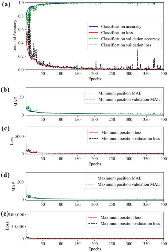
Figure 5.
(a) Classification loss and accuracy with the training epochs in the training process. (b,c) are the mean absolute error (MAE) and the loss of begin position of magnetic anomaly with the training epochs, respectively. (d,e) are the MAE and the loss of end position of magnetic anomaly with the training epochs, respectively.
To evaluate the detection performance of the model, 2800 test samples from the data set ECS_D1 are used. After selecting threshold value (tv), several evaluation metrics, including precision, recall and F1-score, are applied for evaluating the model performance. Precision is defined as the proportion of correctly predicted positives to all predicted positives. Recall is defined as the proportion of correctly predicted positives to all actual positives. F1-score is a harmonic average between precision and recall, which combines these two parameters to eliminate effects of unbalanced sample size for different classes. The precision (), recall () and F1-score are defined as follows:
where is the number of true positives, is the number of false positives and is the number of false negatives.
In order to select the best threshold value for the detection results, the precision, recall and F1-score are calculated using different threshold values (Figure 6). We selected the confidence threshold value of 0.45 responding to the maximum F1-score of 0.985 (Figure 6). Figure 7 shows the predicted results of test sets at a threshold value of 0.45, and its precision and recall are 0.9754 and 0.9948, respectively. Figure 8 shows the six representative samples from the test set. The trained model works very well for SCMAs with different shapes. Although the beginning or end position of predicted area deviates considerably from the true area (Figure 8a–d), these deviations, mostly by less than 20 sample points (Figure 9), are tolerable and acceptable.
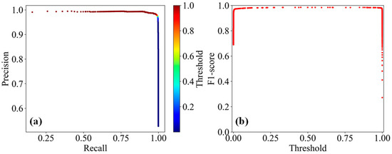
Figure 6.
(a) Precision-recall curve and (b) the F1-score curve calculated from the test set ECS_D1. The different colors in (a) represent the different threshold values. At threshold value 0.45, the precision, recall and F1-score are 0.9754, 0.9948 and 0.985, respectively.
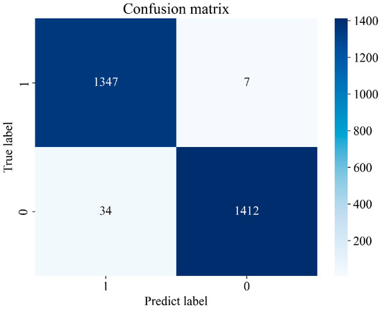
Figure 7.
Table of confusion matrix from the test set ECS_D1. The TP, FN, FP and TN are equal to 1347, 7, 34 and 1412, respectively.
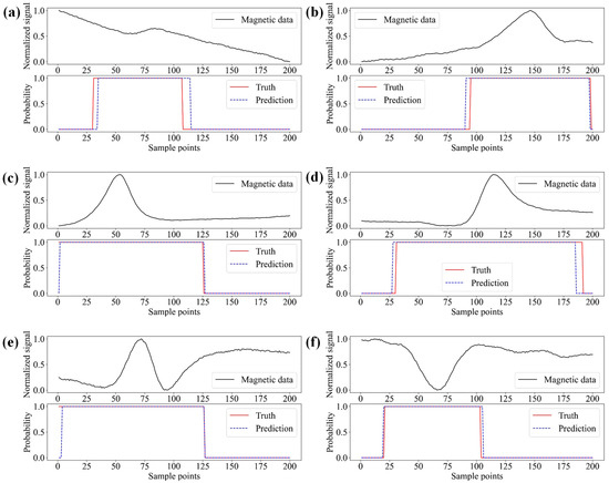
Figure 8.
Detection results using the trained model on some samples in the test set ECS_D1. Each normalized magnetic signal is 200 sample points. Each panel (a–f) shows normalized magnetic signal on top and comparison results of predictions and truths for magnetic anomaly signal detection at the bottom. The blue dashed line represents the prediction label. The red line represents the true label. Normalized signal is calculated by the formula: Normalized signal = (signal − Min)/(Max − Min) with point by point, where Min is the minimum value of signal and Max is the maximum value of signal.
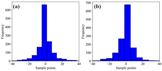
Figure 9.
The frequency distributions of predicted deviations of begin (a) and end (b) position. Mostly prediction position errors are less than 20 sample points.
3.4. Application to Other Regions
In order to test the generalization ability of the model, 200 submarine cable magnetic signals in data set ECS_D1 and eight submarine cable magnetic signals in data set SCS_D are used for recognition. Before testing the data, we need to ensure that the range of 200 sampling points can contain all kinds of SCMAs, which is the sample length assumption of model training. Therefore, the samples of data set SCS_D are resampled at 2 s interval, so as to ensure that the length of samples can contain different kinds of SCMAs.
To predict the samples of data set ECS_D2, the window size is 200 sampling points and the window slide step is 20 sampling points. After predicting each sample, a series of abnormal regions are obtained. Abnormal regions are selected by the non-maximum suppression method, and the IoU value is set as 0.01. The IoU value and window slide step are determined based on the experience value of multiple tests. If the predicted region intersects with labeled region, and the length of the intersecting region divided by the length of labeled region is greater than 0.5, it is considered TP; otherwise, it is FN. If the predicted region does not intersect with the labeled region, it is FP. Accordingly, the recall, precision and F1-score value under different thresholds are calculated.
According to the precision-recall curve and the F1-score curve (Figure 10), we selected the threshold of 0.995 to perform the task. The precision, recall and F1-score for model to the data set ECS_D2 are 0.943, 0.982 and 0.962 respectively. Figure 11 shows the prediction results of the SCMAs in the data set ECS_D2. The model can accurately identify magnetic anomaly signals of different shapes based on different background fields.
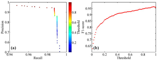
Figure 10.
(a) Precision-recall curve and (b) the F1-score curve calculated from the data set ECS_D2. The different colors of the subfigure (a) represent the different threshold values.
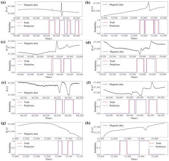
Figure 11.
Comparison of prediction and true labels of SCMAs from data set ECS_D2 by the trained model. Each panel (a–h) shows raw magnetic signal on top and comparison results of predictions and truths for magnetic anomaly signal detection at the bottom. The red line indicates the true label. The blue dashed line indicates the prediction label. B on the vertical axis represents the magnetic induction intensity.
For samples of the data set SCS_D, the window sliding step is 20 sampling points, the IoU is 0.01, and the threshold value is 0.99 to predict the region of SCMAs. The predicted results are shown in Figure 12, which can basically identify all possible magnetic abnormal regions of the submarine cable.
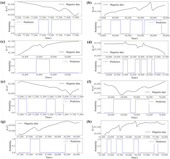
Figure 12.
Prediction results of SCMAs from the data set SCS_D by the trained model. Each panel (a–h) shows raw magnetic signal on top and prediction results for magnetic anomaly signal detection at the bottom. The blue dashed line indicates the prediction label. B on the vertical axis represents the magnetic induction intensity.
In the collected field data, some SCMAs are not easy to distinguish by manual labeling, and may be missed or misjudged in manual interpretation. In the magnetic signal of the dataset ECS_D2 (Figure 13a–c), the analyst labels the magnetic anomaly as a single anomaly, which is actually formed by the superposition of multiple magnetic anomalies; however, the deep learning model can accurately distinguish it. In Figure 13d, because the abnormal signal is not obvious, the analyst missed the SCMA signal, but the deep learning model can fill the missed magnetic anomaly. Automatic recognition of SCMAs through deep learning models can reduce manual interpretation errors and improve the efficiency and accuracy of interpretation.
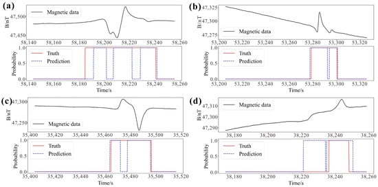
Figure 13.
Comparison of prediction and true results of SCMAs from data set ECS_D2 by the trained model. The red line represents the true label. The blue dashed line represents the prediction label. B on the vertical axis represents the magnetic induction intensity. (a–c) show the artificial misinterpretation of superimposed magnetic anomalies, which can be distinguished using deep learning method. (d) shows the omission of non-obvious magnetic anomalies by manual interpretation, which can be identified by deep learning method.
4. Discussion
In order to study the effect of different blocks on the efficiency of MTCNN model, we remove LSTM block, residual blocks and residual + LSTM blocks, which are denoted as models ReLSTM, ReRes and ReResLSTM, respectively. The maximum F1-score of the test data from the data set ECS_D1 is used to measure the efficiency of the model, and the average of five tests was taken to compare and evaluate.
The ReLSTM model adds residual blocks compared with the ReResLSTM model. The residual blocks significantly improve the ability to extract higher-level features, ensure the stability of the gradient in the model training process, and improve the F1-score of the ReResLSTM model by 0.1265 (Table 2). The ReRes model adds an LSTM block compared with the ReResLSTM model. The LSTM block can learn the internal relationship of the time series characteristics of magnetic anomaly signals. The F1-score of the ReRes model is improved by 0.1215 compared with the ReResLSTM model (Table 2). Combining the advantages of the LSTM and residual blocks, the constructed MTCNN model can reach the optimal F1-score of 0.9795 (Table 2).

Table 2.
F1-scores of different trained models.
The magnetic data collected in the East China Sea are from the submarine power cable, while the magnetic data collected in the South China Sea are from the submarine optical cable. Moreover, most of the data collected in the East China Sea are perpendicular to the direction of the submarine cable, while the data collected in the South China Sea are mostly oblique to the direction of the submarine cable. Due to differences in collection methods or instruments, there are differences in the magnetic anomaly characteristics between the submarine power cable and the submarine optical cable from different regions. The model was trained using the magnetic data of submarine power cables in the East China Sea. The trained model obtained good recognition results on the magnetic data of submarine optical cables in the South China Sea (Figure 12). This indicates that the model has strong generalization ability for SCMAs, and the proposed model is suitable for detecting various types of submarine cables containing ferromagnetism.
The magnetic anomaly recognition model proposed in this article can also be applied in other magnetic anomaly detection fields, such as mineral resource exploration, water conservation and hydropower engineering surveys, underground pipeline and buried object exploration, search and rescue operations, etc. Since the magnetic anomaly characteristics of submarine cables in this study may be different from those of data in other relevant fields, the training process can be simplified by transfer learning. A small part of magnetic anomaly data in relevant fields can be used to train the model by fine-tuning, and finally a model that can recognize magnetic anomalies in other fields is obtained.
5. Summary
In this study, we propose a MTCNN model to realize the synchronous detection of SCMAs and abnormal region positioning. The proposed network model contains a shared feature extraction backbone and three branches. The residual blocks are added to the shared feature extraction backbone to ensure that the model can extract rich high-level features and ensure gradient stability in the training process. The LSTM block is added to the classification task, learning the internal relationship of the magnetic anomaly signal time series, to improve the ability of recognition for magnetic anomalies.
The F1-score of the newly proposed model can reach 0.985 in the test set ECS_D1, and the F1-score in the test set ECS_D2 still remains at 0.962. In the SCS_D data set, the SCMAs can still be accurately identified. Through the above tests and analysis of field data sets in different regions, the generalization performance and processing ability of the MTCNN model are proved. The increase in field data of SCMAs with different characteristics in the future is expected to further enhance the model’s generalization ability.
The newly proposed model can help analysts for SCMAs to automatically recognize them, reduce the probability of erroneous judgments and omissions, and improve the efficiency and accuracy of interpretation. In addition, the SCMA recognition model is also expected to be applied to other fields of magnetic anomaly automatic recognition by means of transfer learning.
Author Contributions
Conceptualization, Y.W.; Methodology, Y.L.; Formal analysis, G.L.; Investigation, Y.W.; Resources, Y.W., L.Y., P.Z., J.K., W.Y., J.W. and Z.X.; Data curation, L.Y., P.Z., J.W. and Z.X.; Writing—original draft, Y.L.; Writing—review & editing, Y.L., Y.W. and G.L.; Visualization, Y.L. All authors have read and agreed to the published version of the manuscript.
Funding
This research is supported by the National Natural Science Foundation of China (Grant No. 42076060), Zhejiang Provincial Geological Special Funds of China for Comprehensive Geological Survey of Zhejiang Province Coastal Zone at Taizhou City and Key Laboratory of Marine Environmental Survey Technology and Application, Ministry of Natural Resources (MESTA-2021-D010), the Bureau of Science and Technology of Zhoushan (No. 2023C81011).
Institutional Review Board Statement
Not applicable.
Informed Consent Statement
Not applicable.
Data Availability Statement
If researchers are interested in our research, they can contact the relevant authors (L.Y., E-mail: 18867623008@163.com, J.K., E-mail: yangjj0812@163.com, W.Y., E-mail: lzheyuan@163.com, J.W., E-mail: wjq53521@gmail.com, Z.X., E-mail: rocsoul@163.com and P.Z., E-mail: zhoupuzhi@smst.gz.cn) to obtain permission, and then contact the author Y.L. (liuyutao@iscas.ac.cn) to obtain the relevant data sets.
Acknowledgments
We thank Jianxiang Zhang and Rui Rui for fruitful discussions. We appreciate the Zhejiang Institute of Marine Geology Survey of China, the South China Sea Marine Survey and the Technology Center of the State Oceanic Administration for providing the field data. The authors thank the editors and reviewers for their comments and constructive suggestions.
Conflicts of Interest
The authors declare no conflict of interest.
Correction Statement
This article has been republished with a minor correction to the Funding statement. This change does not affect the scientific content of the article.
References
- Yu, B.; Liu, Y.; Zhai, G.; Bian, G.; Xiao, F. Magnetic detection method for seabed cable in marine engineering surveying. Geo-Spat. Inf. Sci. 2007, 10, 186–190. [Google Scholar] [CrossRef]
- Zhou, P.; Li, Z.; Shen, Z.; Yin, Z.; Lu, X.; He, X.; Dong, C. Research and application of magnetic detection technology for submarine optical cable. Acta Sci. Nat. Univ. Sunyatseni 2021, 60, 100–110. (In Chinese) [Google Scholar]
- Chen, X.; Zhang, Y. Application study of proton magnetometer to detect submarine cable. Opt. Commun. Technol. 2015, 39, 33–35. (In Chinese) [Google Scholar]
- Ginzburg, B.; Frumkis, L.; Kaplan, B. Processing of magnetic scalar gradiometer signals using orthonormalized functions. Sens. Actuators A Phys. 2002, 102, 67–75. [Google Scholar] [CrossRef]
- Ginzburg, B.; Frumkis, L.; Kaplan, B. An efficient method for processing scalar magnetic gradiometer signals. Sens. Actuators A Phys. 2004, 114, 73–79. [Google Scholar] [CrossRef]
- Ginzburg, B.; Frumkis, L.; Salomonski, N.; Kaplan, B. Optimization of scalar magnetic gradiometer signal processing. Sens. Actuators A Phys. 2005, 121, 88–94. [Google Scholar]
- Fan, L.; Kang, C.; Hu, H.; Zhang, X.; Liu, J.; Liu, X.; Wang, H. Gradient signals analysis of scalar magnetic anomaly using orthonormal basis functions. Meas. Sci. Technol. 2020, 31, 115105. [Google Scholar] [CrossRef]
- Nie, X.; Pan, Z.; Zhang, D.; Zhou, H.; Chen, M.; Zhang, W. Energy detection based on undecimated discrete wavelet transform and its application in magnetic anomaly detection. PLoS ONE 2014, 2014, e110829. [Google Scholar] [CrossRef] [PubMed]
- Sheinker, A.; Shkalim, A.; Salomonski, N.; Ginzburg, B.; Frumkis, L.; Kaplan, B. Processing of a scalar magnetometer signal contaminated by 1/fα noise. Sens. Actuators A Phys. 2007, 138, 105–111. [Google Scholar] [CrossRef]
- Nie, X.; Pan, Z.; Zhang, W. Wavelet-Based Adaptive Detection of Magnetic Anomaly Signal Contaminated by 1/f Noise. Appl. Mech. Mater. 2014, 599, 1812–1815. [Google Scholar] [CrossRef]
- Nie, X.; Pan, Z.; Zhang, W. Wavelet Based Noise Reduction for Magnetic Anomaly Signal Contaminated by 1/f Noise. Adv. Mater. Res. 2014, 889, 776–779. [Google Scholar] [CrossRef]
- Wan, C.; Pan, M.; Zhang, Q.; Wu, F.; Pan, L.; Sun, X. Magnetic anomaly detection based on stochastic resonance. Sens. Actuators A Phys. 2018, 278, 11–17. [Google Scholar] [CrossRef]
- Sheinker, A.; Moldwin, M.B. Magnetic anomaly detection (MAD) of ferromagnetic pipelines using principal component analysis (PCA). Meas. Sci. Technol. 2016, 27, 045104. [Google Scholar] [CrossRef]
- Wang, Y.; Han, Q.; Zhao, G.; Li, M.; Zhan, D.; Li, Q. A deep neural network based method for magnetic anomaly detection. IET Sci. Meas. Technol. 2022, 16, 50–58. [Google Scholar] [CrossRef]
- Zhang, K. Research on Characteristic Analysis and Detection Method of Weak Magnetic Anomaly Signal. Master’s Thesis, University of Electronic Science and Technology of China, Chengdu, China, 2019; pp. 78–88. (In Chinese). [Google Scholar]
- Zhao, G. Research on Interference Mitigation and Target Detection of Airborne Magnetic Anomaly Detection. Ph.D. Thesis, Harbin Institute of Technology, Harbin, China, 2019; pp. 120–126. (In Chinese). [Google Scholar]
- Hochreiter, S.; Schmidhuber, J. Long Short-Term Memory. Neural Comput. 1997, 9, 1735–1780. [Google Scholar] [CrossRef] [PubMed]
- He, K.; Zhang, X.; Ren, S.; Sun, J. Deep Residual Learning for Image Recognition. In Proceedings of the IEEE Conference on Computer Vision and Pattern Recognition, Las Vegas, NV, USA, 27–30 June 2016; pp. 770–778. [Google Scholar]
- Nair, V.; Hinton, G.E. Rectified Linear Units Improve Restricted Boltzmann Machines. In Proceedings of the 27th International Conference on Machine Learning, Haifa, Israel, 21–24 June 2010; pp. 807–814. [Google Scholar]
- Neubeck, A.; Van Gool, L. Efficient Non-Maximum Suppression. In Proceedings of the International Conference on Pattern Recognition, Hong Kong, China, 20–24 August 2006; Volume 3, pp. 850–855. [Google Scholar]
- Redmon, J.; Divvala, S.; Girshick, R.; Farhadi, A. You Only Look Once: Unified, Real-Time Object Detection. In Proceedings of the IEEE Conference on Computer Vision and Pattern Recognition, Las Vegas, NV, USA, 27–30 June 2016; pp. 779–788. [Google Scholar]
- Ren, S.; He, K.; Girshick, R.; Sun, J. Faster R-CNN: Towards Real-Time Object Detection with Region Proposal Networks. IEEE Trans. Pattern Anal. Mach. Intell. 2017, 39, 1137–1149. [Google Scholar] [CrossRef] [PubMed]
- Ioffe, S.; Szegedy, C. Batch Normalization: Accelerating Deep Network Training by Reducing Internal Covariate Shift. In Proceedings of the International Conference on Machine Learning, Lille, France, 6–11 July 2015; pp. 448–456. [Google Scholar]
- Mousavi, S.M.; Zhu, W.; Sheng, Y.; Beroza, G.C. CRED: A Deep Residual Network of Convolutional and Recurrent Units for Earthquake Signal Detection. Sci. Rep. 2019, 9, 10267. [Google Scholar] [CrossRef] [PubMed]
- Zhou, Y.; Yue, H.; Kong, Q.; Zhou, S. Hybrid Event Detection and Phase-Picking Algorithm Using Convolutional and Recurrent Neural Networks. Seismol. Res. Lett. 2019, 90, 1079–1087. [Google Scholar] [CrossRef]
- Ke, L.; Wang, Q.; Jiang, C. Arrhythmia classification based on convolutional long short term memory network. J. Electron. Inf. Technol. 2020, 42, 1990–1998. (In Chinese) [Google Scholar]
- Kingma, D.P.; Ba, J.L. Adam: A method for stochastic optimization. arXiv 2014, arXiv:1412.6980. [Google Scholar]
Disclaimer/Publisher’s Note: The statements, opinions and data contained in all publications are solely those of the individual author(s) and contributor(s) and not of MDPI and/or the editor(s). MDPI and/or the editor(s) disclaim responsibility for any injury to people or property resulting from any ideas, methods, instructions or products referred to in the content. |
© 2023 by the authors. Licensee MDPI, Basel, Switzerland. This article is an open access article distributed under the terms and conditions of the Creative Commons Attribution (CC BY) license (https://creativecommons.org/licenses/by/4.0/).