Research on the Cooperative Scheduling of ARMGs and AGVs in a Sea–Rail Automated Container Terminal under the Rail-in-Port Model

Abstract

Reasonable scheduling of a train’s loading and unloading equipment can reduce the energy consumption of production operations; this has great value for the green development of terminals. The collaborative scheduling model of the Automated Rail Mounted Gantry (ARMG) and Automated Guided Vehicle (AGV) is used to minimize the energy consumption of equipment in a scenario of a vertical railway entering a port and a shared storage yard existing between the port and railway under the mixed operation mode of “train–ship” and “train–yard–ship”. According to the characteristics of the model, the two-layer scheduling rule and the self-adaptive chaos genetic algorithm (SCGA) were proposed to solve the problem of placing the ARMG and the AGV on the same schedule. Simulation experiments verified the effectiveness of the model and algorithm. The effects of the delayed arrival of vessels, the proportion of “transshipment” containers, and the number of automated ARMGs and AGVs on total energy consumption were analyzed. The results showed that when all containers are “train–ship” containers, the number of ARMG and AGV at 1:4 will minimize the total operational energy consumption. Furthermore, as ships take longer to arrive, reducing the number of AGVs can cut energy use by 15% for the same number of ARMG.

1. Introduction

The logistics industry is rapidly evolving with the advancement of technology and the trend towards economic globalization [1]. Ports, as crucial links connecting land and sea, play an indispensable role in the global logistics system. According to UNCTAD, ships transport more than 80% of the world’s trade. Sea–rail intermodal transport has become a critical measure of port development. By combining the advantages of sea and rail transportation, sea–rail intermodal transport can reduce transportation costs and shorten the time of the whole logistics transport. According to the World Bank, sea–rail intermodal transport can save 10–30% of costs as compared to sea transport alone [2].

The “Annual Report on the Development of China’s Container Industry and Intermodal Transport in 2021” highlights that the proportion of container sea–rail intermodal transport volume to port container throughput in 2021 was only 2.7%, which is significantly lower than the 20–40% found in developed countries. In order to increase the proportion of sea–rail intermodal transport and solve the problem of the “middle kilometer” of sea–rail intermodal transport, a project of a unique railway line into the port has been proposed to connect sea and rail transport through railway-dedicated lines into the port (rail-in-port) to achieve a seamless connection between the port and the railway [3]. Railway loading and unloading lines are introduced within the automated terminals, and the process of changing containers between sea and rail transport in trains and ports can all be completed in the ports. Some typical ports include the Port of Long Beach, the Port of Los Angeles, and the Port of Beilun in Ningbo. Among them, the Port of Long Beach has achieved “railway into the port” for automated terminal operations, and it has a layout mode where the railway is parallel to the port. China has built many automated container terminals in recent years, such as the Shanghai Yangshan Port IV automated terminal and Qingdao Port, but none of them are sea–rail automated terminals. Beibu Gulf Port is currently developing China’s first sea–rail automated terminal, but there is still a long way to go for automated terminals and integrated railway operations. In the sea–rail intermodal transport of containers, resource allocation and cooperative scheduling of multiple equipment in sea–rail intermodal ports under the railway entry mode are urgent problems to be solved. Therefore, this paper aims to address the problem of coordinated scheduling of multi-equipment in automated sea–rail terminals to guide the production and operation of automated terminals in China.

Wang [4] divided the layout of the railway line entry into the port into two types of design: parallel and vertical access to the dock by the railway line. After the railway line enters the port, a separate railway yard can be set up in the railway operation area, or the railway can share a yard with the port. Therefore, the layout of the railway into the port can be divided into four types of design:

• Parallel railway entering a port and a separate railway station existing between the port and railway;
• Parallel railway entering a port and a shared storage yard existing between the port and railway;
• Vertical railway entering a port and a separate railway station existing between the port and railway;
• Vertical railway entering a port and a shared storage yard existing between the port and railway.

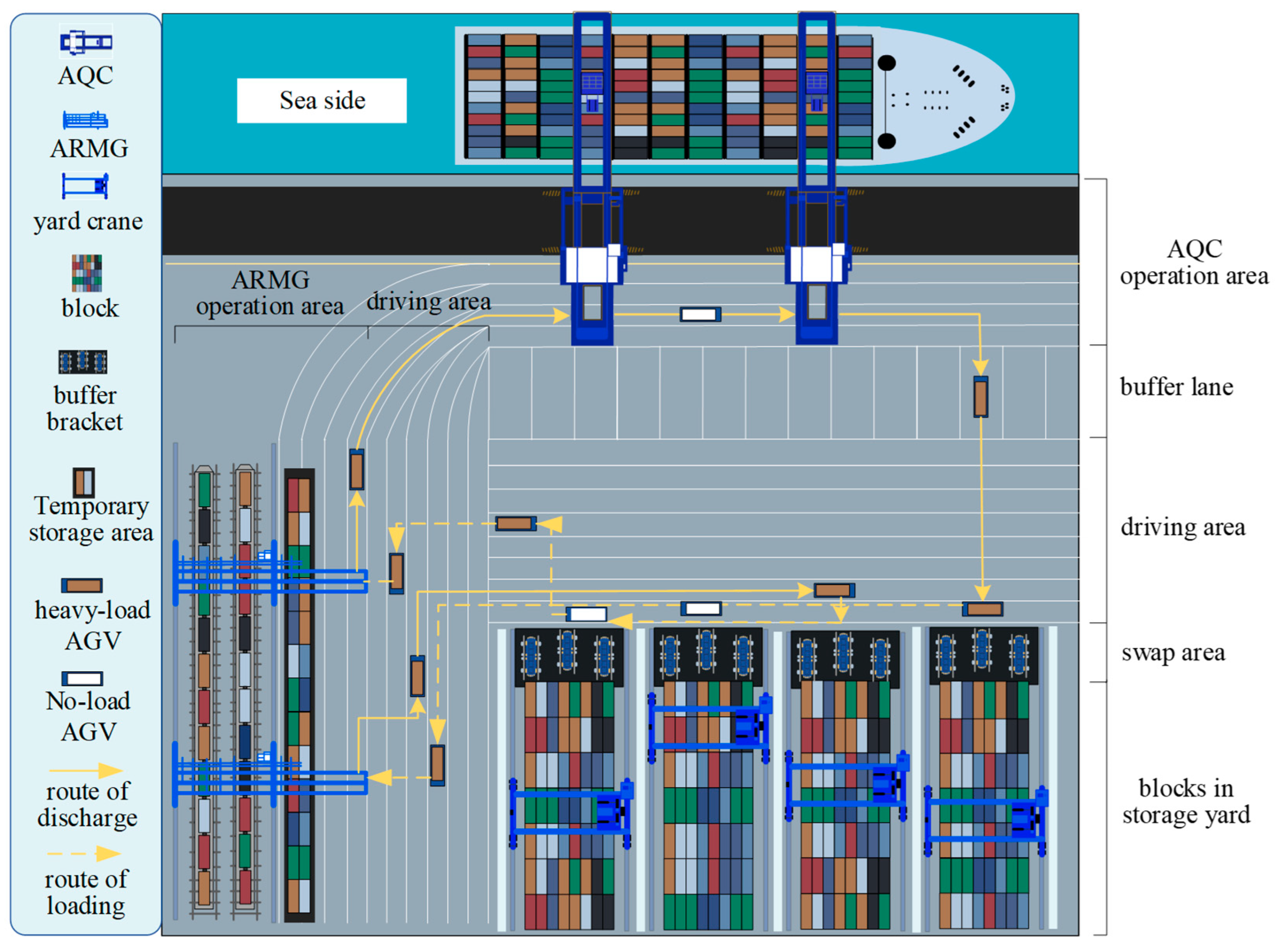
Due to limited port space and shoreline length, the layout mode of a vertical railway entering a port has become prevalent. However, current research in this area has primarily focused on the mode of a parallel railway entering a port, but more attention must be given to the vertical railway entering a port. In addition, Hu [5] proposed a yard-sharing strategy that involves sharing port and rail yards. This approach enables container reloading processes within the port while conserving space and maximizing the utilization of resources. This paper will focus on the fourth layout model which is based on a vertical railway entering a port and a shared storage yard between the port and the railway. The plan layout is shown in Figure 1.

Results of the research concerning the above issues, with particular emphasis on sea-rail intermodal transport with rail access, are discussed below. Sources of information on this subject are included in

Table 1. Literature sources used in the article.

Problems Presented in the Literature and Model	Sources
The necessity and feasibility of developing sea–rail intermodal transport	[1]
The relationship between logistics performance and trade	[2]
The “middle kilometer” of sea–rail intermodal transport	[3]
Layout and operation of sea–rail transport infrastructure	[4]
Save space and maximize the utilization of space resources	[5]
Storage space allocation and handling operation under “train–ship” operation mode	[6,7]
Integrated scheduling of equipment under “train–yard–ship” operation mode	[8]
Integrated scheduling of equipment in hybrid operation mode	[9]
Collaborative scheduling model for devices with time efficiency as optimization goal.	[10,11,12,13]
Collaborative scheduling model of quay crane/yard crane and AGV with energy consumption	[14,15,16]
The proposed genetic algorithm	[17,18,19,20]
The genetic algorithm solution problem	[21,22]
Genetic algorithm for solving crane scheduling with interference	[23]
Improvement of genetic algorithm	[24,25,26]
Priority assignment of equipment	[27]
Adaptive crossover and variance improvement genetic algorithm	[28,29]
Characteristics of chaotic algorithms	[30,31]
Highlight the disadvantages of the genetic algorithm	[32]

.

Most studies on equipment scheduling in sea–rail ports are based on the arrangement of railway loading lines parallel to the port with separate railway yards. Chang [6] investigates the collaborative scheduling of rail-mounted gantry cranes, inner trucks, and quay cranes in a “train–vessel” operation mode in which obtaining the most time for loading and unloading operations is the optimization objective. Zhao [7] reviewed how railway containers are organized in real-world situations by looking at how the container center station and the port station work together. Container transport organizations should try to meet the “train–ship” direct loading and unloading conditions, as well as reduce the high fees associated with storage time mentioned in the conclusion. Yan [8] transforms the problem of yard bridges, trucks, and rail cranes into a mixed integrated planning model based on the “train–yard–ship” mode of operation in port rail handling areas to reduce the maximum completion time and total waiting time for all equipment. Li [9] proposed that incorporating “train–ship” and “train–yard–ship” hybrid operation modes could improve the efficiency of port operations. To achieve this, Li developed a collaborative scheduling model for rail cranes and container trucks, with the optimization objective of minimizing time. It’s worth noting that this study is not specifically focused on automated container terminals for sea–rail intermodal transport. The equipment in the parallel port arrangement of railway lines has been studied extensively in the literature [6,7,8,9].

However, further research is needed to investigate the scheduling of port equipment under the vertical port arrangement of the railway. Considering the practical situation of China’s ports and the increasing demand for railway access to automated terminals, it is necessary to explore different port access modes.

Some scholars have studied the scheduling problem of container handling equipment in automated terminals and central railway stations. Zhang [10] created a quay scheduling model that prioritizes time efficiency as the optimization objective. The study highlights the significance of task prioritization and non-interference constraints in achieving this goal. Considering the uncertainty of ship arrival time as well as loading and unloading quantity, a rail crane scheduling model was established by He [11] to minimize delay times. Li [12] established a rail crane scheduling model to minimize train residence time by considering constraints such as the moving time window and safe distance of rail cranes. Wang [13] proposed an RMGC scheduling optimization model to minimize the no-load time of RMGC in the handling task, and its goal was to determine an optimal handling sequence. Yan [8] took the minimum operation time and total waiting time of all equipment as the optimization objective to study the comprehensive scheduling problem of loading and unloading equipment in the container terminals’ railway loading and unloading area. Some scholars have also conducted related research to reduce the energy consumption of the automation terminal operation equipment. Yue [14] examined the issue of collaborative scheduling for quay cranes and AGVs in automated container terminals, with the aim of optimizing energy consumption. The study emphasized that meeting the available laytime of ships in the port is a prerequisite for reducing operational energy consumption. Zhao [15] investigated the collaborative scheduling problem between rail cranes and AGVs, considering constraints such as rail crane interference, AGV travel routes, and quantity configurations. The optimization objectives were to minimize the total operating time and energy consumption. Xing [16] developed a mixed integer programming model considering the total construction period of the crane and the minimum energy consumption of the AGV. The study addressed the cooperative scheduling problem among the quay crane, AGV, and yard crane. Adjustment heuristics and branch constraint programs were used to optimize the task assignment of AGVs and yard cranes.

The Genetic Algorithm is an adaptive global optimization search algorithm that mimics how organisms in their natural environment pass on traits and evolve over time. It borrows concepts from biogenetics and enhances individual adaptability through natural selection, crossover, and mutation. Professor J.H. Holland [17] in the USA proposed the first genetic algorithms. They originated in the 1960s with research on natural and artificial adaptive systems. In the 1970s, K.A. De Jong [18,19] conducted numerous experiments on computers using genetic algorithms for purely numerical function optimization calculations, and in the 1980s, D.E. Goldberg [20] developed genetic algorithms based on a series of research studies. As genetic algorithms have a relatively complete mathematical model and theory, many researchers have employed them to solve NP-hard problems. For example, Ganji [21] used a genetic algorithm to solve the continuous berth allocation problem, and Gan [22] tackled the automated container terminal AGV collaborative scheduling problem using a genetic algorithm. However, genetic algorithms face issues such as slow convergence and quickly falling into local optimum solutions. Hence, some researchers have improved the genetic algorithm. Han [23] studied and resolved the crane scheduling problem with disturbance constraints using a genetic algorithm, demonstrating that a genetic algorithm can solve equipment scheduling issues. Fuertes [24] modified the stochastic parameters of the genetic algorithm using chaotic sequences and experimentally demonstrated the performance of this chaotic genetic algorithm. To obtain the best solution for shop scheduling in a reasonable time, Wang [25] proposed an adaptive multiple-population genetic algorithm and verified its effectiveness through testing, showing that the adaptive crossover probability can expand the search range. Bao [26] suggested that adaptive crossover and mutation rates could enhance the ability to search for the global optimum. The chaos algorithm and adaptive strategy can improve the genetic algorithm. Based on this, we propose a self-adaptive chaos genetic algorithm to solve the collaborative scheduling problem of the ARMG and the AGV.

In summary, the current sea–rail intermodal automated terminals mainly adopt the parallel railway line layout mode and set up independent railway yards. The majority of research on collaborative scheduling of multiple equipment with the optimization goal of minimizing operational energy consumption has been focused on automated container terminals. In contrast, less research is carried out on sea–rail intermodal automated container terminals. With the adoption of peak carbon and carbon neutral targets, green and low-carbon development has become a crucial transformation direction for all industries. The port industry, as a vital component of the transportation sector, contributes significantly to carbon emissions. The optimization of ports involves a comprehensive approach that considers efficiency, cost, and energy consumption. Due to space constraints, this paper concentrates on researching the optimization problem of energy consumption in equipment scheduling. Specifically, the paper aims to tackle the energy efficiency optimization problem in ports by reducing the energy consumption of equipment operations while ensuring efficiency.

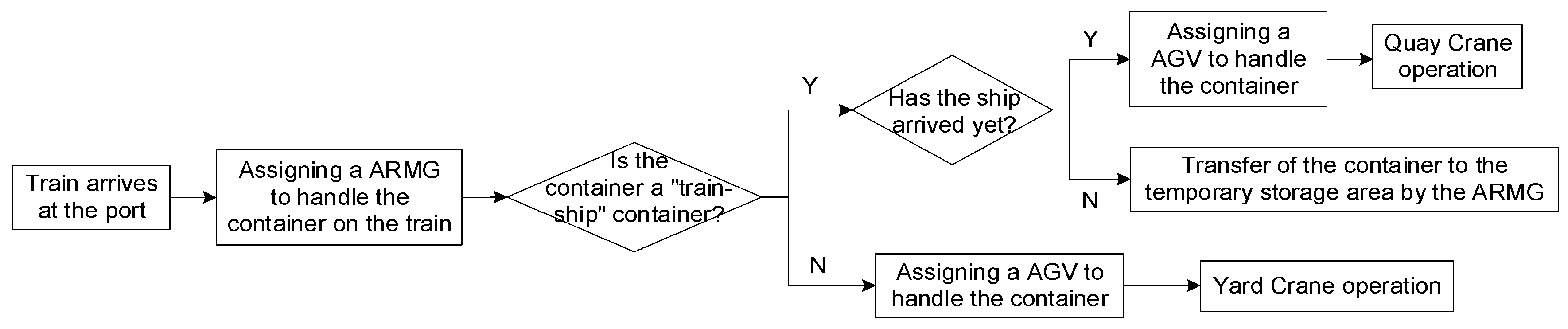
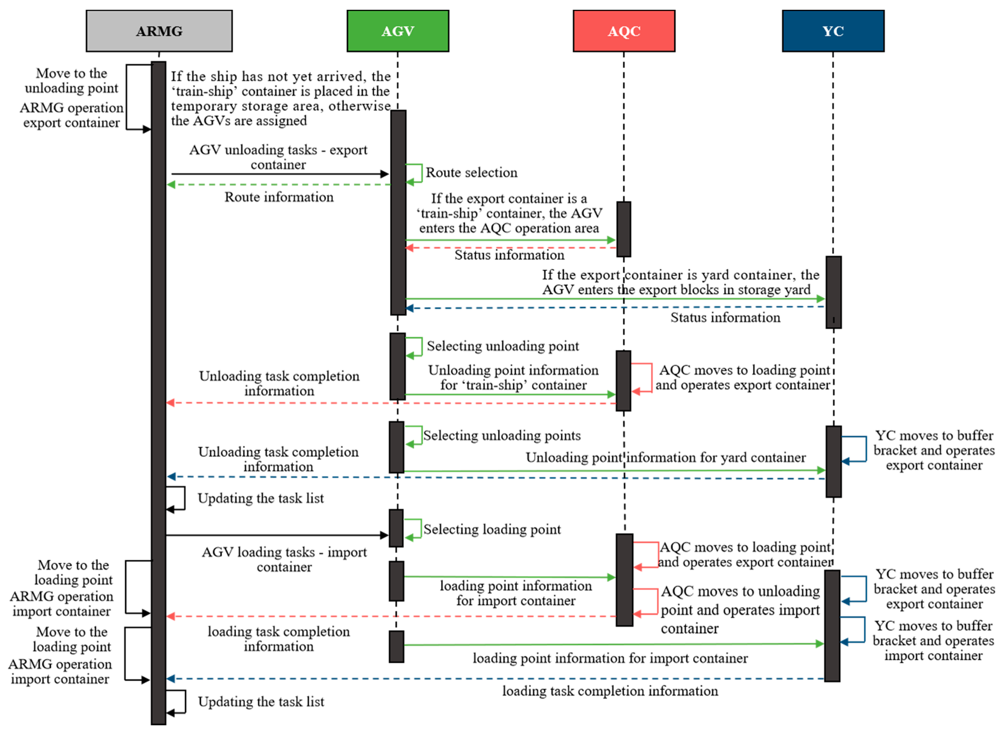
In the production and operation of sea–rail automated terminals, due to various uncertainties such as weather, natural disasters, and port congestion, the schedules of ships and trains may partially overlap. To enhance the container turnover speed, sea–rail ports utilize this time window for some containers to adopt the “train–ship” mode of operation and move them to the front of the terminal. The remaining containers follow the “train–yard–ship” operation and proceed to yard storage, which aligns with the principle of efficient handling of sea–rail container operations. This paper leverages this time window overlap to reduce the times of secondary loading and unloading operations, thereby cutting down the operational energy consumption of ARMGs and AGVs in the sea–rail intermodal container transfer process. The optimization objective is to construct a collaborative scheduling model for ARMGs and AGVs under the mixed operation mode to determine the operation sequence of ARMGs and AGVs, as well as the energy consumption of their operations.

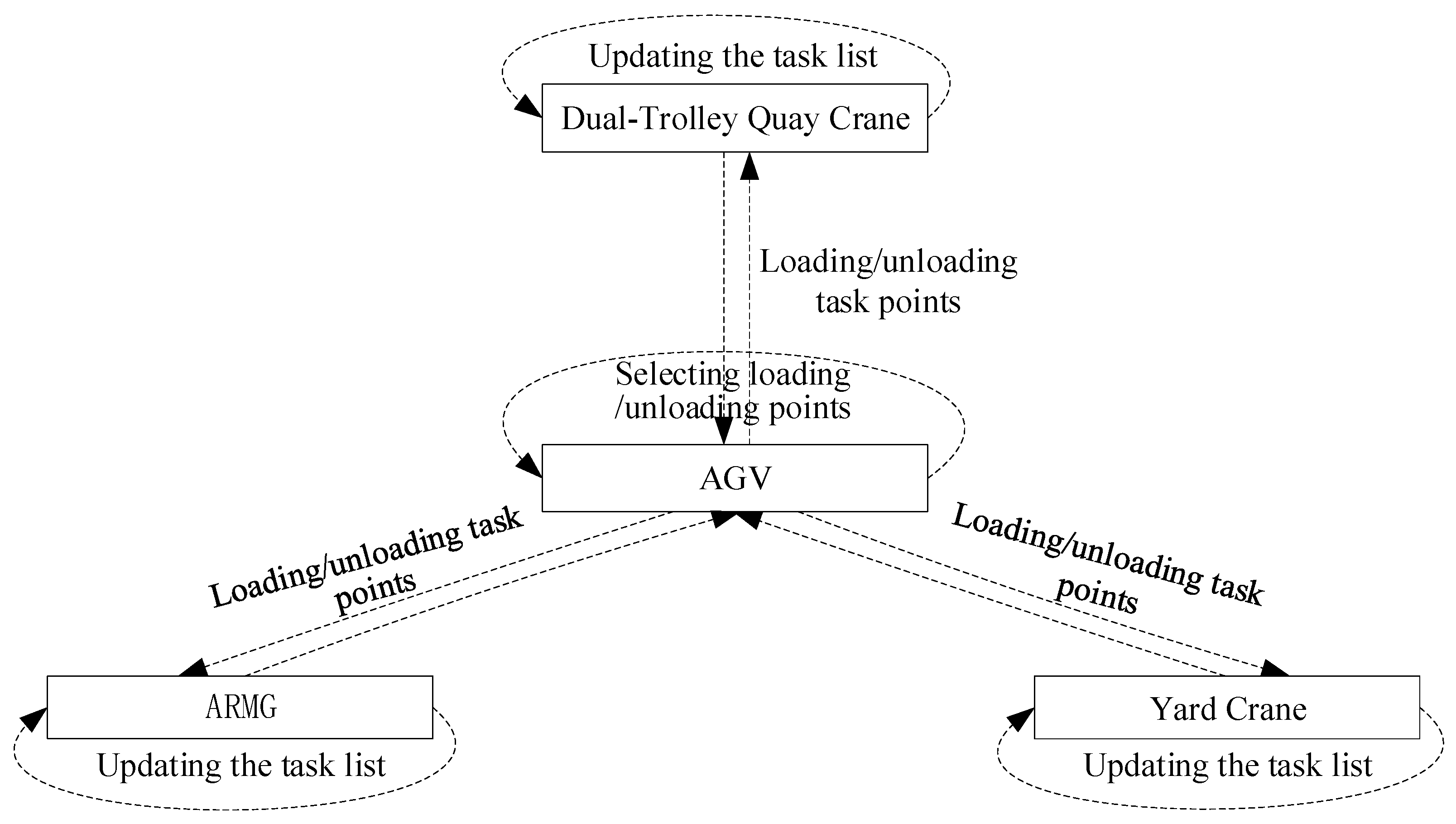
The complexity of the collaborative scheduling problem significantly increases given that it involves multiple areas of operation, including the ARMG operation area, the automated quay crane (AQC) operation area, the blocks in the storage yard, and is also affected by uncertainty in the arrival time of ships and trains. Accordingly, this paper aims to analyze the logical coupling relationships between the AGV, ARMG, AQC, and yard cranes and multi-equipment collaborative scheduling in the mixed operation mode. The collaborative scheduling model of ARMGs and AGVs is next established in mixed operation mode, and according to the problem and model characteristics, we design the self-adaptive chaos genetic algorithm (SCGA) to solve it. The optimal ratio of ARMGs to AGVs that minimizes the total operational energy consumption is derived through simulation experiments. The optimal ratio of ARMGs to AGVs is also obtained for different delayed ship arrival and “transshipment” container ratios. The research results significantly affect the scheduling of multiple equipment at sea–rail automated terminals and the development of green ports that use the rail-in-port model.

This paper makes a valuable contribution to the development of a collaborative dispatching model for ARMG and AGV in the hybrid operation mode of “train–ship” and “train–yard–ship,” with energy consumption as the optimization objective. This problem presents a direct cross-system multi-equipment scheduling challenge between the port and the railway, which urgently needs to be addressed in sea–rail automated container terminals. While scholars have explored coordinated scheduling of equipment under the railway entry mode, more research is necessary on the cross-system coordinated scheduling of multiple pieces of equipment in beach intermodal automated container terminals with a vertical railway entry and a shared yard mode.

To address this issue, the paper introduces a practical adaptive chaos genetic algorithm to solve the coordinated scheduling model of ARMG and AGV in mixed “train–ship” and “train–yard–ship” operation modes. Although adaptive genetic algorithms have been studied in [23,24] and chaotic genetic algorithms in [25,26], practical adaptive chaotic genetic algorithms have not been fully applied until now, making this another significant contribution of the paper.

2. Problem Description and Mathematical Model

2.1. Problem Description

The railway port of entry completes the sea–rail intermodal container changing operation involving several operation areas, including the ARMG operation area, the AQC operation area, and blocks in the storage yard. AGVs connect the loading and unloading equipment of each operation area. The ARMG’s primary function is to transport containers either from the train to the AGV or a temporary storage area, or from the AGV to the train. Meanwhile, the AGV is responsible for moving containers from the area where the ARMG operates to the area where the quay crane or yard is located.

When the sea–rail container is changed inside the port, the interrelationships between the ARMG, AGV, AQC, and YC are those shown in Figure 2. The ARMG, the AQC, and the YC need the loading and unloading point information of the AGV, and the AGV needs the status information of the ARMG, the AQC, and the YC to make decisions.

The operation mode of the sea–rail intermodal transport port can be divided into “train–ship” and “train–yard–ship” according to the overlap of train and ship schedules. Furthermore, the sea–rail intermodal transport container can be divided into “train–ship” and “transshipment” containers. Upon the train’s arrival at the port, the ARMG will commence the unloading operation. In the case of a “train–ship” container, the AGV will transport it to the AQC operation area. Conversely, if it is a “transshipment” container, the AGV will move it to the yard. Since the arrival time of the ship is often uncertain, “train–ship” containers may be temporarily placed in the storage area yard until the ship arrives. Subsequently, after the ship’s arrival, the ARMG and AGV will collaborate in the AQC operation area. The sea–rail container handling operation process in mixed operation mode is illustrated in Figure 3.

The intermodal containers within the train–ship operation time window will be transferred to the ship, while the remaining ones not within the time window will be stored in the yard. In this mode, the dynamic scheduling information of sea–rail intermodal containers is shown in Figure 4.

Once the train has entered the port, the ARMG unloads the export containers from the train. If the export container is a “train–ship” container and the ship and the train arrive simultaneously, the AGV will transport the export “train–ship” container from the ARMG unloading point to the AQC loading point. After completing the delivery of the unloaded container, the AGV will drive back empty to the AQC unloading point/import block in the storage yard to pick up the import container. In the event that the ship has yet to arrive at the port, and the export container is a “train–ship” container, the ARMG will unload the container onto the temporary storage area, and there is no need to allocate the AGV at this time. If the export container is a yard container, the AGV will transport the export yard container from the ARMG unloading point to the import block in the storage yard. After completing the delivery of the export container, the AGV drives empty to the import block in the storage yard to pick up the import container. After picking up the imported container, the AGV will review at the ARMG’s status information to select the loading and unloading point and move the imported container to the ARMG’s loading and unloading point.

The rail-in-port mode allows for the complete sea–rail container change within the port. The coordinated scheduling plan of ARMGs and AGVs is one of the critical factors affecting the level of coordination of train loading and unloading operations. The coordinated scheduling plan of ARMGs and AGVs can determine their operation sequence and operation time, which is the basis for ensuring the implementation of train loading and unloading operations. At the same time, the configuration of ARMGs and AGVs also affects the time trains stay in the port and the waiting time of ARMGs and AGVs, which in turn affects the operational energy consumption in the production process. Frequent turning on and off of the ARMG and AGV can significantly impact their life and reliability. Thus, terminal operating equipment is typically utilized in standby mode, where it generates energy while idle. An unreasonable scheduling scheme will increase the waiting time of the ARMGs and AGVs in the port production process, leading to an increase in the waiting energy consumption of the ARMGs and AGVs. Hence, studying the coordinated scheduling scheme of ARMGs and AGVs under the rail-in-port mode can reduce operating time and energy use and make port production more efficient.

In the rail-in-port mode, imported and exported containers are categorized as either “train–ship” and “transshipment”. Considering the complexity of the problem, this paper focuses solely on the collaborative scheduling of ARMGs and AGVs during the unloading operation. The optimization aims to establish a collaborative scheduling model for ARMGs and AGVs that considers practical constraints such as the “train–ship” operation time window, the safety distance between railway cranes, and the heavy unladen load of railway cranes and AGVs. The ultimate objective is to determine the order of railway crane and AGV operations, as well as the total operational energy consumption of ARMGs and AGVs.

This study is based on the following assumptions: (1) Only export container operations are considered during the statistical period, and the allowable operating hours for ships and trains are known; (2) All containers are 40-foot containers; (3) There is no waiting time for AGVs under the AQC and YC; (4) The performance of all rail cranes is the same; (5) The performance of all AGVs is the same; (6) The maximum capacity of the temporary storage area is sufficient; (7) There are no uncertainties, such as path conflicts, during AGV transport.

2.2. Mathematical Model

All the sets, parameters, auxiliary variables, and decision variables are shown in

Table 2. Sets, parameters, and variables.

Sets
$N_1$	represents the set of ‘train-ship’ containers, indexed by i
$N_2$	represents the set of “transshipment” containers, indexed by j
$N$	represents the concatenation of the set of ‘train-ship’ containers and the set of yard containers, indexed by k
$R$	represents the set of ARMGs, indexed by r
$V$	represents the set of AGVs, indexed by v
$B$	represents the set of carriages bays indexed by b
$\phi$	represents the set of tasks that cannot be worked on at the same time $\phi =\{(k,k^{\prime })|k,k^{\prime }\in N,\left|l_{k^{\prime }}-l_k\right|\le {\mathrm{l}}_{saf}\}$
parameters
$C_r^f$	Energy consumption per hour of heavy load for one ARMG
$C_r^o$	Energy consumption per hour of no-load for one ARMG
$C_r^m$	Energy consumption per hour of movement of one ARMG
$C_v^f$	Energy consumption per hour of heavy load for one AGV
$C_v^o$	Energy consumption per hour of no-load for one AGV
$C_v^w$	Energy consumption per hour of waiting for an AGV
$l_k$	Location of the container’s carriage
$\tau$	Time taken to move one carriage by ARMG
$l_{saf}$	Safety margin for ARMG
$t_p$	Unit time for containers at temporary storage point P for ARMG operations
$O$	An infinitely large number
$f_1$	Total operational energy consumption of ARMGs
Auxiliary variables
$f_2$	Total operational energy consumption of AGVs
$t_{rf}^k$	Heavy load time for gantry trolley operation of ARMG r
$t_{ro}^k$	No-load time for gantry trolley operation of ARMG r
$Q_p^k$	The number of containers to be operated at the temporary storage point P of the corresponding carriage when operating container k
$t_v^k$	AGV v transporting container k with heavy load time
$t_{vk}^o$	AGV v transporting container k with no-load time
${\mathrm{t}}_{v{i}^{\prime }}^o$	The empty drive time for the AGV to the ARMG operating area to pick up ‘train-ship’ container i’, when the AGV operation to pick up ‘train-ship’ container i is completed
${\mathrm{t}}_{vj}^o$	The empty drive time for the AGV to the ARMG operating area to pick up yard container j, when the AGV operation to pick up ‘train-ship’ container i is completed
${\mathrm{t}}_{v{j}^{\prime }}^o$	The empty drive time for the AGV to the ARMG operating area to pick up yard container j, when the AGV operation to pick up yard container j’ is completed
${\varpi }_{vk}^r$	Waiting time under the ARMG when AGV v transports container k
$p_r^k$	Planned operating time for the ARMG r to lift the container k from the train and place it on the AGV
$q_r^k$	Actual operating time for the ARMG r to lift the container k from the train and place it on the AGV
$T_{ship}$	Actual time of arrival of the ship
$T_v^k$	The time for the AGV to reach the ARMG when it will unload container k
$T_Q^i$	The time when the AGV v transports the ‘train-ship’ container i from the ARMG to the AQC
$T_S^j$	The time when the AGV v transports the yard container i from the ARMG to the export block in storage yard
Decision variables
$x_r^k$	$x_r^k=\{\begin{array}{l}1,\mathrm{i}\mathrm{f} \mathrm{container} \mathrm{k} \mathrm{is} \mathrm{operated} \mathrm{by} \mathrm{ARMG} \mathrm{r}\\ 0,\begin{array}{c}\mathrm{otherwise}\end{array}\end{array}$
$y_v^k$	$y_v^k=\{\begin{array}{l}1,\mathrm{i}\mathrm{f} \mathrm{container} \mathrm{k} \mathrm{is} \mathrm{operated} \mathrm{by} \mathrm{AGV} \mathrm{v}\\ 0,\begin{array}{c}\mathrm{otherwise}\end{array}\end{array}$
$w_r^{k{k}^{\prime }}$	$w_r^{k{k}^{\prime }}=\{\begin{array}{l}1,\mathrm{i}\mathrm{f} \mathrm{ARMG} \mathrm{r} \mathrm{operates} \mathrm{on} \mathrm{k} \mathrm{and} {\mathrm{k}}^{\prime } \mathrm{and} \mathrm{k},{\mathrm{k}}^{\prime } \mathrm{is} \mathrm{a} \mathrm{sequential} \mathrm{sequence}\\ 0,\begin{array}{c}\mathrm{otherwise}\end{array}\end{array}$
$w_v^{ij}$	$w_v^{k{k}^{\prime }}=\{\begin{array}{l}1,\mathrm{i}\mathrm{f} \mathrm{AGV} \mathrm{v} \mathrm{operates} \mathrm{on} \mathrm{k} \mathrm{and} {\mathrm{k}}^{\prime } \mathrm{and} \mathrm{k},{\mathrm{k}}^{\prime } \mathrm{is} \mathrm{a} \mathrm{sequential} \mathrm{sequence}\\ 0,\begin{array}{c}\mathrm{otherwise}\end{array}\end{array}$
$Z_{rp}^k$	$Z_{rp}^i=\{\begin{array}{l}1,\mathrm{i}\mathrm{f} \mathrm{the} \mathrm{corresponding} \mathrm{point} \mathrm{P} \mathrm{has} \mathrm{containers} \mathrm{when} \mathrm{the} \mathrm{ARMG} \mathrm{r} \mathrm{works} \mathrm{k}\\ 0,\begin{array}{c}\mathrm{otherwise}\end{array}\end{array}$

.

Equation (1) is an objective function that aims to minimize the total energy consumption of ARMGs and AGVs. Equation (2) represents the total operational energy consumption of the ARMGs, including the heavy-load energy consumption, the no-load energy consumption, and the movement energy consumption of the ARMGs. Equation (3) represents the total operational energy consumption of the AGV, including the heavy-load energy consumption, the no-load energy consumption, and the AGV waiting for the ARMG.

$$\min f=f_1+f_2,$$

(1)

$$f_1=C_r^f\cdot {\displaystyle \sum _{r\in R}{\displaystyle \sum _{k\in N}\left(x_r^k{t}_{rf}^k+Q_p^k{t}_p\right)}}+C_r^o\cdot {\displaystyle \sum _{r\in R}{\displaystyle \sum _{k\in N}{x}_r^k{t}_{ro}^k}}+C_r^m\cdot {\displaystyle \sum _{r\in R}{\displaystyle \sum _{k,k^{\prime }\in N}|l_{k^{\prime }}-l_k|}}\cdot \tau ,$$

(2)

$$f_2=C_v^f\cdot {\displaystyle \sum _{v\in V}{\displaystyle \sum _{k\in N}{y}_v^k{t}_v^k}}+C_v^o\cdot {\displaystyle \sum _{v\in V}{\displaystyle \sum _{k\in N}{y}_v^k{t}_{vk}^o}}+C_v^w\cdot {\displaystyle \sum _{v\in V}{\displaystyle \sum _{k\in N}{\varpi }_{vk}^r}}.$$

(3)

Equation (4) indicates that each export container has only an ARMG crane operating. Equations (5) and (6) indicate that each ARMG has only one pre- and post-sequence task. Equation (7) indicates that each export container has only one AGV completing the operation. Equations (8) and (9) indicate that each AGV has only one pre- and post-sequence task.

$${\displaystyle \sum _{k\in N}{x}_r^k}=1,\forall r\in R,$$

(4)

$${\displaystyle \sum _{r\in R}{\displaystyle \sum _{k,k^{\prime }\in N}{w}_r^{k{k}^{\prime }}=1,\forall k^{\prime }\in }}N,$$

(5)

$${\displaystyle \sum _{r\in R}{\displaystyle \sum _{k^{\prime }\in N}{w}_r^{k{k}^{\prime }}=1,\forall k\in }}N,$$

(6)

$${\displaystyle \sum _{k\in N}{y}_v^k}=1,\forall v\in V,$$

(7)

$${\displaystyle \sum _{v\in V}{\displaystyle \sum _{k^{\prime }\in N}{w}_v^{k{k}^{\prime }}=1,\forall k\in }}N,$$

(8)

$${\displaystyle \sum _{v\in V}{\displaystyle \sum _{k\in N}{w}_v^{k{k}^{\prime }}=1,\forall k^{\prime }\in }}N.$$

(9)

Equation (10) is a constraint relationship in which the actual operating time of the ARMG is not earlier than the planned operating time of the container k. Equation (11) indicates an ARMG safety distance constraint. When the export containers k and k’ cannot be operated simultaneously, the ARMG r needs to move to the safety margin after operating k before the ARMG r’ can start operating the container k’.

$$q_r^k-p_r^k\ge 0,\forall k\in N,r\in R,$$

(10)

$$p_{r^{\prime }}^{k^{\prime }}\ge p_r^k+t_{rf}^k+t_{ro}^k+l_{saf}\cdot \tau ,\forall r,r^{\prime }\in R,(k,k^{\prime })\in \phi .$$

(11)

Equation (12) means that the start of the subsequent task of the ARMG operation is after the previous task. Equation (13) means that if the actual arrival of the ship is later than the actual operation of the ARMG, the ‘train–ship’ container will be put into the temporary storage area first.

$$p_r^{k^{\prime }}-(p_r^k+t_{rf}^k+t_{ro}^k+|l_{k^{\prime }}-l_k|\cdot t_b)\ge {(\mathrm{w}}_r^{k{k}^{\prime }}-1)*O,\forall r\in R,k,k^{\prime }\in N,$$

(12)

$$Q_p^i=\{\begin{array}{c}{Q}_p^i+1,\begin{array}{cc}if& q_r^i\ge T_{ship}\end{array}\\ Q_p^i,otherwise\end{array},\forall r\in R,k\in N_1.$$

(13)

Equation (14) implies that if there are containers at the corresponding temporary storage point when the ARMG is operating on the export containers, priority is given to operating on the containers at the temporary storage point to reduce the waiting time of the AGV. Equation (15) establishes that the actual operating time of the ARMG is not later than the arrival time of the AGV, i.e., the ARMG is guaranteed not to wait for the AGV. Equation (16) shows the relationship between how long the ARMG actually operates and when the AGV arrives.

$$p_r^{k^{\prime }}=\{\begin{array}{l}{p}_r^k+Q_p^k\cdot t_p,\mathrm{if} z_{rp}^k=1\\ p_r^k+t_{rf}^k+t_{ro}^k+|l_j-l_i|\cdot \tau ,otherwise\end{array},\forall r\in R,k,k^{\prime }\in N,$$

(14)

$$p_r^k-T_v^k\ge (1-x_v^k)*O,\forall r\in R,k\in N,v\in V,$$

(15)

$$q_r^k=\max \left\{p_r^k,T_v^k\right\},\forall r\in R,k\in N,v\in V.$$

(16)

Equation (17) indicates the heavy load time of the AGV transporting the export container k. If k is a “train–ship” container, the heavy load time is the time the AGV transports from the ARMG to the AQC, and if k is a yard container, the heavy-load time is the time the AGV transports from the ARMG to the export block in the storage yard. Equations (18)–(20) indicate the idling time of the AGV after operating a “train–ship” container or “transshipment” container and returning from the AQC or the export block in the storage yard to the ARMG operation area to continue operating the next “train–ship” container or “transshipment” container. Equation (21) indicates the idle time of the AGV while operating the next task.

$${\mathrm{t}}_v^k=\{\begin{array}{c}{\mathrm{T}}_Q^i-{\mathrm{T}}_V^i+(1-y_v^i)*O,\begin{array}{cc}if& k\in N_1\end{array}\\ {\mathrm{T}}_s^j-{\mathrm{T}}_V^j+(1-y_v^j)*O,\begin{array}{cc}if& k\in N_2\end{array}\end{array},\forall v\in V,$$

(17)

$${\mathrm{t}}_{vi\prime }^o>({\mathrm{T}}_v^{i^{\prime }}-{\mathrm{T}}_Q^i)+(1-w_v^{i{i}^{\prime }})*O,\forall v\in V,i,i^{\prime }\in N_1,$$

(18)

$${\mathrm{t}}_{vj}^o>({\mathrm{T}}_v^j-{\mathrm{T}}_Q^i)+(1-w_v^{ij})*O,\forall v\in V,i\in N_1,j\in N_2,$$

(19)

$${\mathrm{t}}_{v{j}^{\prime }}^o>({\mathrm{T}}_v^{j^{\prime }}-{\mathrm{T}}_S^j)+(1-w_v^{j{j}^{\prime }})*O,\forall v\in V,j,j^{\prime }\in N_2,$$

(20)

$$t_{v{k}^{\prime }}^o=\{\begin{array}{l}{\mathrm{t}}_{v{i}^{\prime }}^o,\forall v\in V,i,i^{\prime }\in N_1\\ {\mathrm{t}}_{vj}^o,\forall v\in V,i\in N_1,j\in N_2\\ {\mathrm{t}}_{v{j}^{\prime }}^o,\forall v\in V,j,j^{\prime }\in N_2\end{array}.$$

(21)

Equations (22) and (23) represent that the start time of the subsequent task of an AGV operation is at the completion time of the previous task. The completion time of the previous task is when the AGV returns to the ARMG after the task. If the AGV returns to the ARMG earlier, the time the AGV waits for the ARMG must be added. The waiting time is the difference between the actual operating time of the ARMG and the arrival time of the AGV. Equation (24) represents the priority of the next task of the AGV operation, i.e., when the two ARMGs unload the “train–ship” container and the “transshipment” container, respectively, the AGV gives priority to the “train–ship” container operation. Equations (25) and (26) define the parameters and decision variables’ ranges.

$$T_v^{k^{\prime }}-(T_v^k+t_v^k+t_{v{k}^{\prime }}^o)\ge (1-w_v^{k{k}^{\prime }})*O,\forall v\in V,k,k^{\prime }\in N,$$

(22)

$${\varpi }_{v{k}^{\prime }}^r\ge (q_r^{k^{\prime }}+T_v^{k^{\prime }}),\forall v\in V,k^{\prime }\in N,$$

(23)

$$P_{\mathrm{vi}}>P_{vj},\forall v\in V,i\in N_1,j\in N_2,$$

(24)

$$p_r^k\ge 0,T_v^k\ge 0,\forall r\in R,v\in V,k\in N,$$

(25)

$$x_r^k,y_v^k,Z_{rp}^k,w_r^{k{k}^{\prime }},w_v^{k{k}^{\prime }}\in \left\{0,1\right\},\forall k,k^{\prime }\in N,r\in R,v\in V.$$

(26)

3. Self-Adaptive Chaotic Genetic Algorithm

The model mentioned above considers both “train–ship” and “train–yard–ship” modes of operation, which increases its complexity and makes it difficult to solve quickly using traditional genetic algorithms. Li [27] verified that assigning tasks according to equipment priorities can effectively reduce the total operation time of equipment. 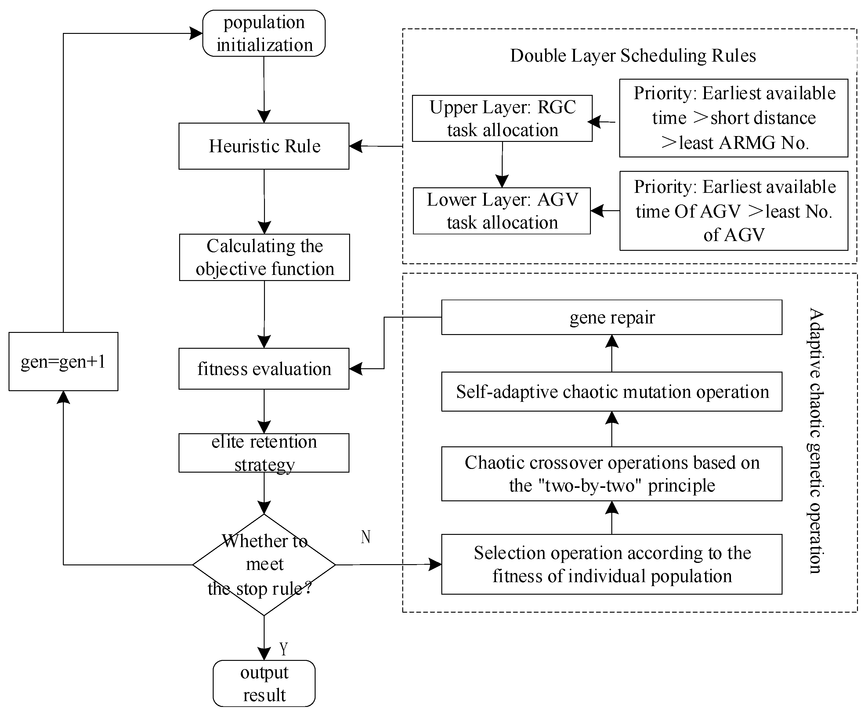Additionally, maintaining population diversity and the convergence of genetic algorithms can be achieved through adaptive crossover and mutation probabilities [28,29]. Therefore, to solve the model, the self-adaptive chaotic genetic algorithm (SCGA) is proposed. First, based on the task attributes of the ARMG and AGV, a double-layer scheduling rule for the ARMG and AGV is designed in the priority order of earliest available time, shortest distance, and the most minor equipment number. The self-adaptive strategies are used to adjust the crossover and mutation operators. Moreover, the ergodic nature of the chaotic algorithm and its sensitivity [30,31] to initial conditions are utilized to overcome the problems of poor local searchability and slow convergence of the genetic algorithm [29,32]. The algorithm flow chart is shown in Figure 5.

3.1. Coding of Tasks

The operational tasks are containers on trains and containers in temporary storage areas. The tasks are sorted by actual number coding, with genes on the chromosome corresponding to the operational tasks, with codes such as 1-3-5-8-2-11-6-9-4-12-7-10.

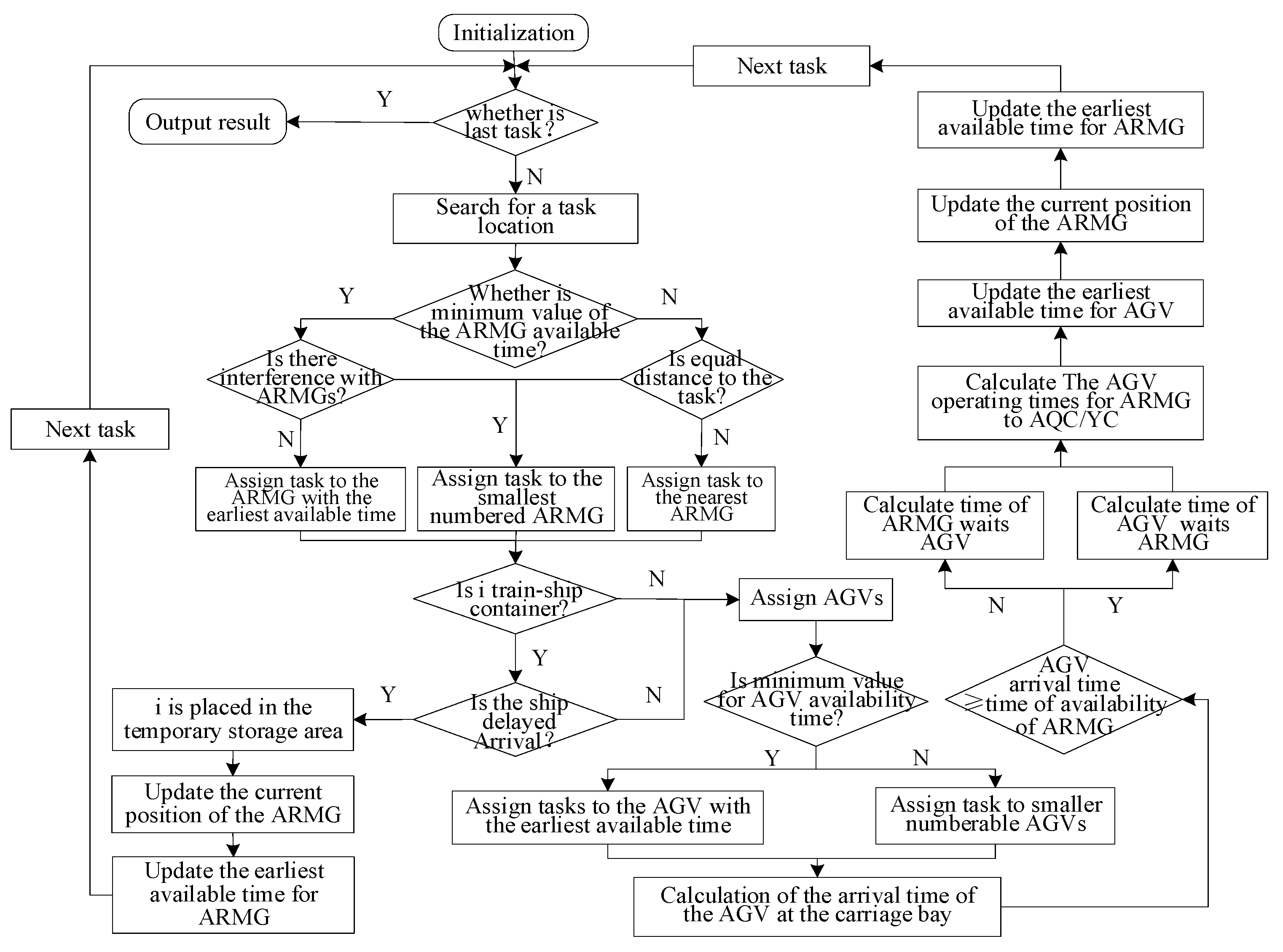
3.2. Double-Layer Scheduling Rules for ARMGs and AGVs

A “two-level scheduling” heuristic rule is designed based on the operational attributes of the ARMG and the AGV, as shown in Figure 6.

The upper layer is the crane scheduling layer. Based on the completion time of the previous task of the ARMG operation, the location of the ARMG where the last task was completed, and the ARMG No., 3*R feature matrices are created to enable control of the ARMGs. Whether the ARMG satisfies the safe margin crossing is determined by Equation (11). The task is assigned to the ARMG in the priority order of earliest available time, ARMG interference, proximity to the task location, and size of ARMG No. When a task is assigned to the ARMG, the feature matrix of the ARMG is updated according to Equations (12)–(14).

The lower layer is the AGV scheduling layer. The AGV is controlled by building a 2*V feature matrix based on the completion time of the previous task and the AGV No. check of the operational attributes of the container. If the container is a “train–ship” container and the ship is delayed in port, the next task is assigned; otherwise, the AGV is assigned according to the priority order of the earliest available time and the smaller AGV No. When a task is assigned to the AGV, the feature matrix of the ARMG is updated according to Equations (17)–(21). Equation (22) should be used to calculate the time for the AGV to wait for the ARMG after the task has been assigned to the ARMG and the AGV. When all tasks have been assigned, the objective function value is calculated according to Equations (1)–(3).

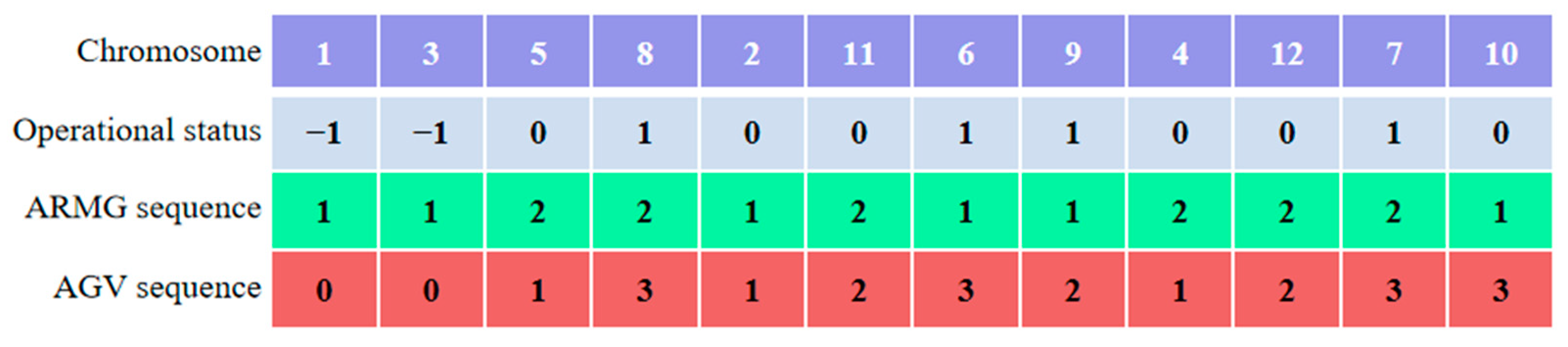
3.3. Chromosome Decoding

The randomly generated chromosome code is as 1-3-5-8-2-11-6-9-4-12-7-10 according to the train–ship schedule and the ship’s delayed arrival time; the sequence of container operation status is as follows: (−1)- (−1) -0-1-0-0-0-1-1-0-0-1-0-1-0-1-1-1. Zero means the container is a “train–ship” container transported by AGV to the AQC. One means the container is a yard container transported by AGV to export blocks in the storage yard. Negative one means that the container is a “train–ship” container. However, the actual time of the ship’s arrival is later than the planned time, so it will be placed into the temporary storage area first and then transported by AGV to the AQC after the ship’s arrival. If two ARMGs and three AGVs are involved in the operation, the chromosome decoding schematic diagram is shown in Figure 7.

After task allocation, the ARMG operation sequence 1-1-2-2-1-2-1-1-1-2-2-1 is obtained, and the AGV operation sequence 0-0-1-3-1-2-3-2-1-2-3-3 is also obtained. Container 1 does not require AGV operation and is operated by ARMG 1 in the temporary storage area for temporary storage. Container 5 is a “train–ship” container to the AQC operated by ARMG 2 in collaboration with AGV 1. ARMG 2, in conjunction with AGV 3, operates transfer container 8 to the export blocks in the storage yard. The operation sequence of ARMG 1 is 1-3-2-6-9-10, the operation sequence of ARMG 2 is 5-8-11-4-12-7, the operation sequence of AGV 1 is 5-2-4, the operation sequence of AGV 2 is 11-9-12, and the operation sequence of AGV 3 is 8-6-7-10.

3.4. Fitness Function

To maintain the ARMG and AGV using the least amount of energy while operating, the inverse of this objective function is used as the adaptation value F.

3.5. Select the Operations

The binary tournament selection operation is employed in this study as it can be easily parallelized and is less likely to become trapped in local optimum conditions during the selection process. First, populations that rank within the bottom 1/10 of the fitness value are eliminated directly, and the remaining populations are selected using the binary tournament method.

3.6. Crossover and Mutation Operations

According to the evolutionary characteristics of the population, the crossover and variation probabilities are dynamically and non-linearly adjusted using trigonometric functions, i.e., the dynamic adaptive crossover and variation probabilities are determined according to Equations (27) and (28). Where $p_c^{\prime }$ and $p_m^{\prime }$ are the crossover and mutation probability parameters, respectively, with the crossover probability taking on the values, the variation probability taking on the values, which denote the average fitness value of the population per generation, the value of the more excellent fitness of the two crossover individuals, and the fitness value of the individual to be mutated.

$$p_c=\{\begin{array}{c}{p}_c^{\prime }+(p_{c\_\max }-p_c^{\prime })\cdot \cos (\frac{f_{avg}-f^{\prime }}{f_{avg}-f_{c\_\min }}\times \frac{\pi }{2}),f^{\prime }<f_{avg}\\ p_c^{\prime }-(p_c^{\prime }-p_{c\_\min })\cdot \sin (\frac{f^{\prime }-f_{avg}}{f_{c\_\max }-f_{avg}}\times \frac{\pi }{2}),f^{\prime }\ge f_{avg}\end{array},$$

(27)

$$p_m=\{\begin{array}{c}{p}_m^{\prime }+(p_{m\_\max }-p_m^{\prime })\cdot \cos (\frac{f_{avg}-f}{f_{avg}-f_{m\_\min }}\times \frac{\pi }{2}),f<f_{avg}\\ p_m^{\prime }-(p_m^{\prime }-p_{m\_\min })\cdot \sin (\frac{f-f_{avg}}{f_{m\_\max }-f_{avg}}\times \frac{\pi }{2}),f\ge f_{avg}\end{array}.$$

(28)

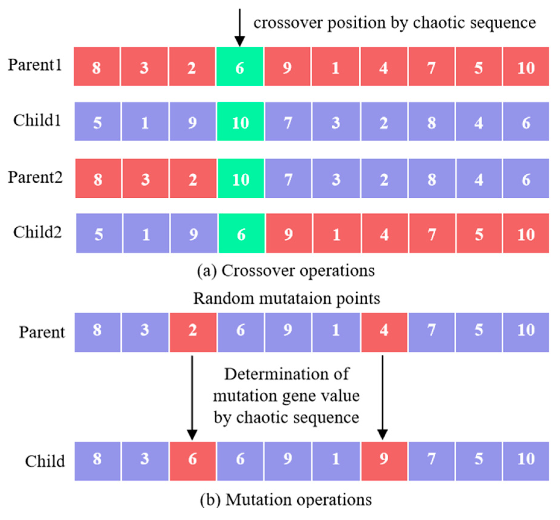
The selected chromosomes use the chaotic single-point crossover to reduce the damage to the chromosomes and to ensure the accuracy of the algorithm’s convergence. In addition, chaotic two-point variation is used to improve local random searchability.

$$x\left(n+1\right)=\mu *x\left(n\right)*\left(1-x\left(n\right)\right)floor\left(N*X_{gen}\right),$$

(29)

$$L_N=floor\left(N*X_{gen}\right).$$

(30)

Crossover operation: After the population fitness values are sorted in descending order, the populations are paired in order, and a positive integer between 2 and N-1 (N is the chromosome size) is generated using the logistic chaos sequence of Equation (29) to determine the location of the crossover point. The specific steps are to generate a random value x(n) from 0 to 1, iterate once according to Equation (29) to generate the chaotic value as the initial value for the next iteration of the chaotic crossover operation, and then determine the location of the crossover point according to Equation (30).

Mutation operation: Two integers in the interval [2, N-1] are randomly generated, and the position of the mutation operation point is determined according to these two generated integers. The specific steps are the initial values of the gene values, N, at the two randomly generated integer positions. Finally, the new gene values after chaotic mutation are obtained using Equations (29) and (30).

To form the new generation population, the new individuals obtained through genetic manipulation are combined with the top 10% of the fitness value of the parent population. The specific operations of crossover and mutation are shown in Figure 8.

3.7. Algorithm Stopping Rule

The algorithm is stopped when the maximum number of iterations is reached or when the value of the objective function does not change for n consecutive generations.

4. Simulation Experiments and Analysis

The simulation experiments are designed to verify the effectiveness of the proposed model and algorithm. The algorithm was written using MATLAB R2016b and solved using an i7-12700H processor with the Windows 10 operating system.

The simulation experiments include the effect of ARMG and AGV configuration, delayed vessel arrival time, and the different container quantities and yard container ratios on operational energy consumption. Through the experiments, the optimal number of ARMGs and AGVs and their scheduling sequence are obtained to minimize the energy consumption of the equipment. In addition, the effects of different delayed arrival times of ships, the number of containers, the percentage of “transshipment” containers, and the configuration of ARMGs and AGVs on energy consumption are also analyzed.

The optimization problem under investigation in this paper is optimized with specific objective functions and constraints that may vary with different inputs. Consequently, simulation experiments were conducted to derive the optimal solution by inputting varying numbers of devices, resulting in the following simulation results.

4.1. Simulation Experiments on the Impact of ARMG and AGV Configurations on Energy Consumption

In the rail-in-port mode, the layout of the automated container terminal is shown in Figure 1, and the cooperative operation relationship between ARMGs and AGVs is shown in Figure 3. Taking the J-terminal of the Port of Long Beach in the United States as a reference, the railway loading and unloading line has three railway tracks, each of which has a maximum capacity of 40 carriages. Temporary storage points are set up in the railway operation area for temporary container storage. There are 6 lanes in the ARMG operation area, each 4 m wide; 5 two-way lanes in the AGV driving area; and 4 blocks in the storage yard, which are 50 m apart. There are 8 two-way lanes from the yard to the AQC operation area, with 27 m of buffer lane lengthways, and 6 lanes in the quayside bridge operation area, each 4 m wide.

Table 3. Parameters of equipment and models.

Parameters	Value	Parameters	Value
Speed of ARMG trolley	85 m/min	$l_{saf}$	1 carriage bay
Travelling speed of ARMG	80 m/min	$C_r^f$	30 kWh/h/unit
Speed of ARMG lift heavy load	15 m/min	$C_r^o$	20 kWh/h/unit
Speed of ARMG lift no load	24 m/min	$C_r^m$	15 kWh/h/unit
$t_p$	1 min	$C_v^f$	21 kWh/h/unit
$v_f$	210 m/min	$C_v^o$	14 kWh/h/unit
$v_o$	350 m/min	$C_v^w$	9 kWh/h/unit

indicates parameters [15,16] related to loading and unloading equipment in the ARMG operation area, and

Table 4. Parameters of SCGA.

Parameters	Value	Parameters	Value
Population size	50	$p_{c\min }$	0.9
Maximum iterations	500	$p_{c\max }$	0.4
$p_c^{\prime }$	0.6	$p_{m\min }$	0.1
$p_m^{\prime }$	0.05	$p_{m\max }$	0.01

represents the parameters of the SCGA algorithm.

Assume that three trains are entering the port simultaneously, each train has a container on the car, and each container is an operational task. Suppose the ratio of direct pick-up boxes to total containers is one. The optimal number of AGVs and the total operation energy consumption of ARMGs and AGVs are obtained by solving the solution when 2–4 ARMGs are configured. The calculation results are shown in

Table 5. Comparison of different scheduling options.

A	V	Maximum Completion Time for ARMGs	Total Energy Consumption		Scheduling Solutions for ARMGs	Start-Finish Time
2	8	92.84	169.37	RGC1	B1-21	0–92.84 min
				RGC2	B22-40	0–79.58 min
3	12	54.67	165.56	RGC1	B1-B14	0–54.67 min
				RGC2	B15-B27	0–52.22 min
				RGC3	B28-B40	0–51.78 min
4	16	65.52	197.91	RGC1	B1-B12	0–65.52 min
				RGC2	B10-B19	0–38.21 min
				RGC3	B20-B30	0–44.56 min
				RGC4	B30-B40	0–41.84 min

.

It can be seen from Table 5 that the total energy consumption of ARMGs and AGVs can be minimized when the number of ARMGs and AGVs is 2, 8 AGVs, 3, 12 AGVs and 4, 16 AGVs. Therefore, when the railway rail crane and AGV are configured at 1:4, the total operational energy consumption of the ARMGs and AGVs is minimized.

When 2–4 ARMGs are configured, the maximum completion time for the ARMGs is 92.84 min, 54.67 min, and 65.52 min, respectively. The increase from two to three ARMGs reduces the maximum completion time and total operational energy consumption. However, when they increase from three to four, the full completion time of the ARMGs increases due to the excessive number of ARMGs, resulting in ARMG interference, which increases the total operation energy consumption.

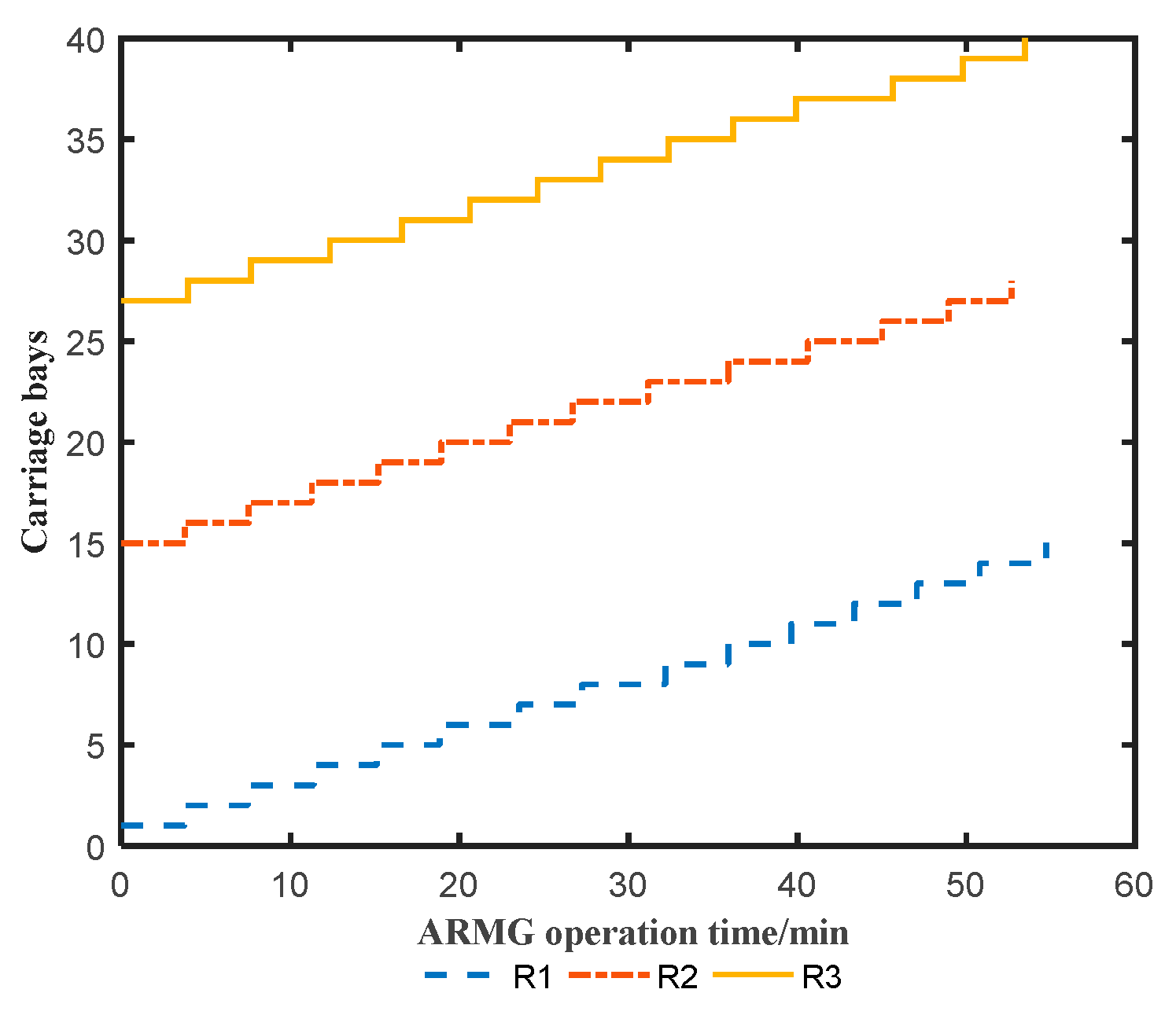
In conclusion, the configuration of three ARMGs and twelve AGVs can shorten the time of trains in the port and minimize the total energy consumption of ARMGs and AGVs. Consequently, three ARMGs and twelve AGVs should be deployed for unloading operations where conditions permit. At this moment, the real-time travel path of the ARMGs between the carriages is shown in Figure 9, and the AGV scheduling results are shown in

Table 6. Scheduling results for AGVs.

AGV No.	Sequence of AGV Operating Containers	AGV No.	Sequence of AGV Operating Containers
1	1-5-17-19-21-23-31-39-48-91-106-114	7	3-12-22-24-26-28-34-42-55-59-63-72-78-86
2	7-43-50-66-70-74-93-99-117	8	14-25-45-88-96-108-113-119
3	30-51-67-71-75-82-94-100-118	9	10-27-65-77-84-92-98-110-120
4	2-9-11-36-47-54-58-62-80-105-111	10	4-6-13-33-35-37-40-87-95-101-107
5	29-44-49-53-57-61-79-104-112	11	8-15-38-46-76-81-89-97-103-109
6	16-20-68-73-83-90-102-116	12	18-30-32-41-52-56-60-64-85-115

. As can be seen from Figure 8, ARMG 1 operates train compartments 1–14, ARMG 2 operates train compartments 15–27, and ARMG 3 operates train compartments 28–40. The route of ARMG’s operation has no intersections, and a safe margin is maintained at all times.

To verify the superiority of SCGA, an improved genetic algorithm (IGA) was designed to compare and analyze it with SCGA. First, for population initialization, three rows and N columns of the initial population (N is the chromosome size, and NIND is the population size) are randomly generated. The three rows represent the container operation, ARMG, and AGV operation sequences. The fitness value is then calculated, and the population is subjected to genetic manipulation. The crossover operation of the literature [15] is used, in which two individuals are randomly selected for the crossover operation, and four new individuals can be generated. After the cross operation is completed, the fitness value is calculated. Fifty percent of the population is eliminated, and then the two-point mutation operation is carried out. The algorithm terminates when the maximum number of iterations is reached.

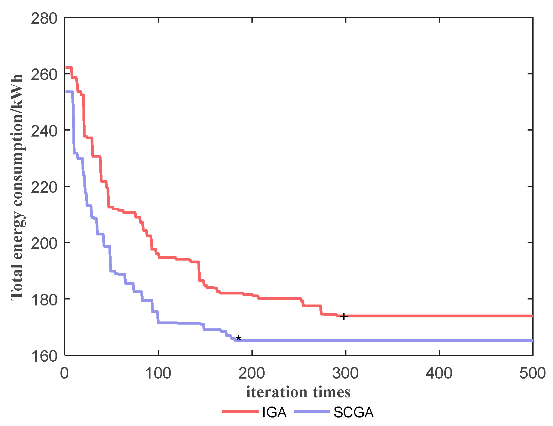
In the configuration of 120 containers, 3 ARMGs and 12 AGVs, SCGA and IGA are used to solve the problem, respectively. The convergence curves of the two algorithms are shown in Figure 10.

Figure 10 shows that SCGA iteration to 182 generations finds the optimal solution to be 165.56 kWh, while iteration to 293 generations of the improved genetic algorithm finds the optimal solution to be 174.01 kWh. The difference between the total energy consumption of SCGA and IGA is 8.45 kWh. Compared with IGA, SCGA has fewer iterations and faster computation speed, indicating that the double-layer scheduling and algorithm-stopping rule in SCGA can make the algorithm converge earlier. Moreover, the proposed self-adaptive strategy and chaotic algorithm can solve the genetic algorithm’s poor local searchability to a certain extent, which makes SCGA better than IGA in terms of results and speed. As a result, SCGA can better solve the cooperative scheduling problem of ARMGs and AGVs in the rail-in-port mode.

4.2. Simulation Experiments on the Impact of Delayed Arrival Times of Ships on Energy Consumption

Factors contributing uncertainty such as weather and port traffic can cause the arrival time of ships to be volatile. When the ship’s arrival time is delayed, the ARMG must place the first “train–ship” containers in the temporary storage area. This, in turn, necessitates the ARMG’s operation on the containers twice upon the ship’s arrival, leading to increased operational energy consumption. To examine the impact of different delayed ship arrival times on operational energy consumption, a simulation experiment was conducted. This involved adjusting the number of AGVs based on the delayed ship arrival times and observing and analyzing the changes in operational energy consumption. The temporary storage area only serves as a buffer, so it can only be occupied for a short time. When all “train–ship” containers have been placed in the temporary storage area, the “tarin–ship” containers must be placed in the storage yard if the ship still needs to dock. Therefore, the maximum delay in the ship’s arrival time is when the last direct container is placed in the temporary storage area.

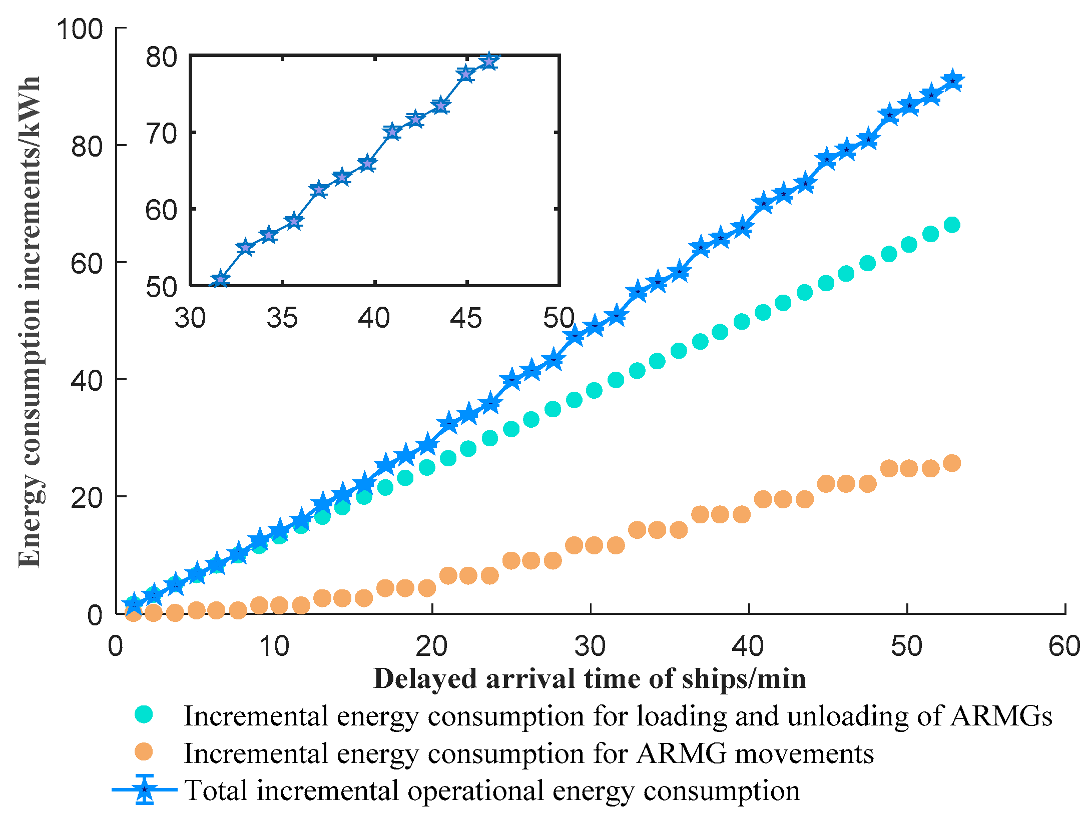
In order to study the influence of a ship’s delayed arrival time on operation energy consumption, the simulation experiment was carried out with 120 “train–ship” containers, 3 ARMGs and 12 AGVs at different ships’ delayed arrival times. The experiment was divided into 14 groups, and each was repeated 20 times. The average value of each group was taken, where $\mathsf{\Delta }T$ was the delayed arrival time of ships and $\mathsf{\Delta }{f}_R$ was the operational energy consumption increment of ARMGs. The experimental results are shown in Figure 11.

As seen from Figure 11, the maximum delay time of the ship is 55.46 min, at which the operational energy consumption increases by 92.82 kWh. It will increase the loading and unloading energy consumption and moving energy consumption of the ARMGs as the delayed arrival time of the ship increases, increasing the total operational energy consumption. The primary cause of the energy consumption increase is the secondary dispatching of ARMGs. Additionally, during the unloading of “train–ship” containers into the temporary storage area, AGV operations are not required. Once the ship arrives at the port, ARMGs and AGVs operate together within the AQC operation area. Thus, when the ship is delayed at the port, maintaining the same number of AGVs will prolong their waiting time for ARMGs, ultimately increasing the energy consumption of AGVs.

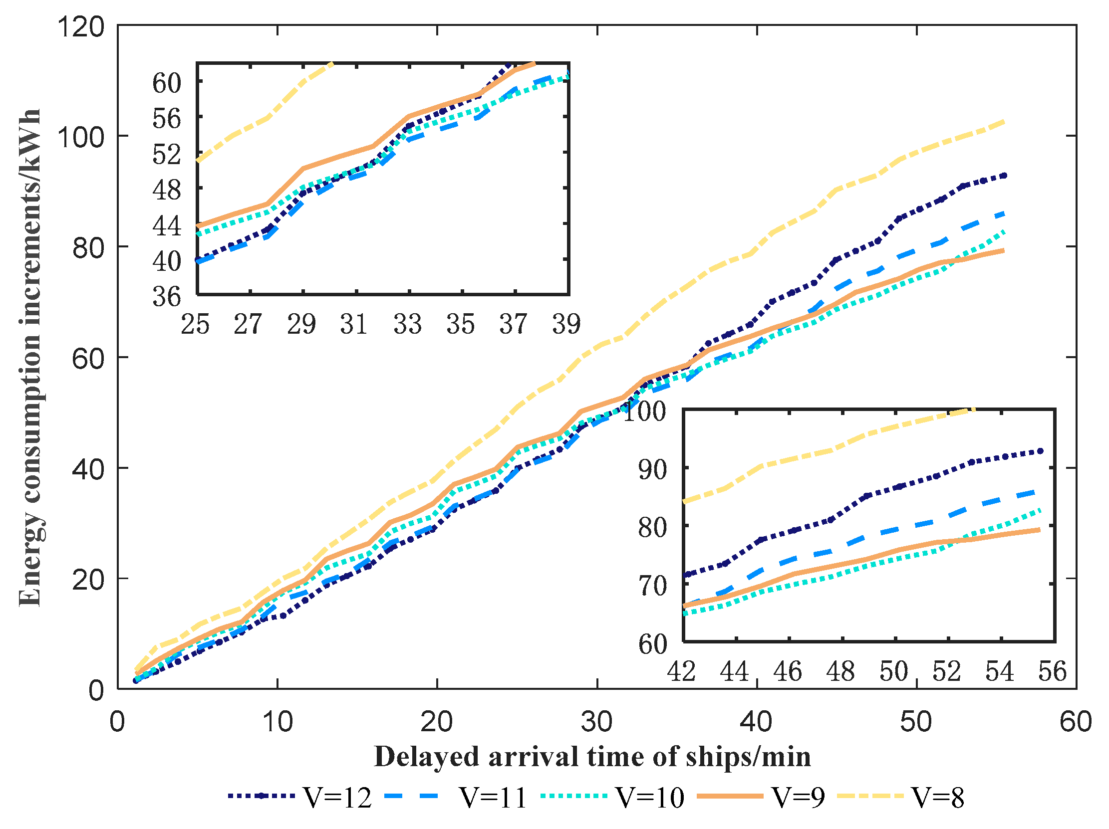
In order to reduce the total operational energy consumption increment of ARMGs and AGVs, the number of containers and ARMGs was kept unchanged in the above experiment, and the number of AGVs was reduced to observe the change in operational energy consumption. The results of the experiment are shown in Figure 12.

As seen from Figure 12, with the delayed arrival time of ships no earlier than 25.02 min, the energy consumption increment configured with 11 AGVs is 2.75 kWh less than that configured with 12 AGVs. In the [25.02, 36.9] range for ship delayed arrival times, energy consumption increments with 10 AGVs are 4.55 kWh lower than with 11 AGVs. When the ship’s delayed arrival time is later than 42.2 min, the energy consumption increment with 9 AGVs is the least at 78.26 kWh, which reduces the energy consumption increment by 15.69% compared with 12 AGVs. Currently, the quantity configuration ratio of the ARMG to the AGV is 1:3. Its configuration of 8 AGVs’ operation consumption increment was higher than 9, 10, 11 and 12 AGV increments in energy consumption.

In conclusion, since ships are coming in later, reducing the number of AGVs can lower the energy that ARMGs and AGVs use to operate. If the ship is late arriving to the port, the equipment can use less energy if the ratio of ARMG to AGV is changed in a way based on the actual time the ship arrives to port.

4.3. Simulation Experiments on the Impact of Different Container Quantities and Yard Container Ratios on Energy Consumption

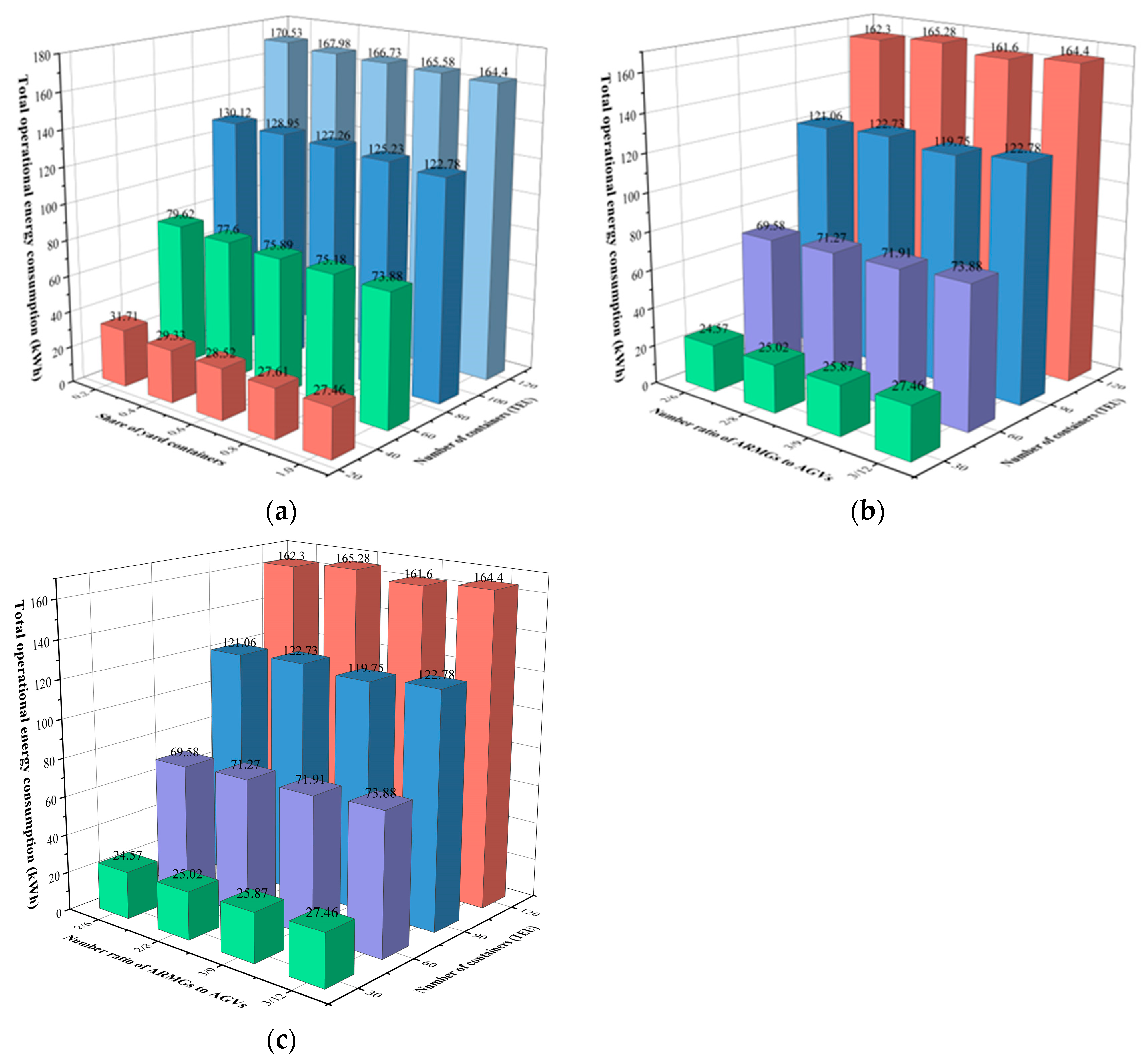
The number and type of containers on the freight train are variable. This paper takes the number of ARMGs and AGVs configured as 2/6, 2/8, 3/9, and 3/12 as examples. The number of containers (30, 60, 90, 120) and the ratio of yard containers (0.2, 0.4, 0.6, 0.8, 1) were adjusted to study the influence of a different number of containers and the ratio of yard containers on the total energy consumption of ARMGs and AGVs. The experiments were conducted in twenty groups; each group was repeated ten times, and the average value was calculated. The yard containers were randomly placed in four export blocks in the storage yard. Moreover, the results are shown in

Table 7. Energy consumption for different containers with different yard containers ratios.

Number of Containers	Ratio of Yard Containers	2ARMGs/6 AGVs		2 ARMGs/8 AGVs		3 ARMGs/9 AGVs		3 ARMGs/12 AGVs
		${\mathit{f}}_1/\mathbf{kWh}$	${\mathit{f}}_2/\mathbf{kWh}$	${\mathit{f}}_1/\mathbf{kWh}$	${\mathit{f}}_2/\mathbf{kWh}$	${\mathit{f}}_1/\mathbf{kWh}$	${\mathit{f}}_2/\mathbf{kWh}$	${\mathit{f}}_1/\mathbf{kWh}$	${\mathit{f}}_2/\mathbf{kWh}$
30	0.2	18.49	10.84	17.36	11.48	19.03	13.43	18.64	13.07
	0.4	17.73	10.32	16.89	10.73	18.28	12.45	17.14	12.19
	0.6	16.59	10.26	16.43	10.44	17.01	11.12	16.73	11.79
	0.8	16.27	9.64	16.33	9.88	16.35	10.78	16.27	11.34
	1	15.77	8.80	15.77	9.25	16.14	9.73	16.14	11.32
60	0.2	34.28	44.40	35.21	44.35	37.35	45.55	35.31	44.31
	0.4	32.83	43.89	33.79	43.45	35.50	44.71	33.98	43.62
	0.6	32.02	41.46	32.53	42.06	33.03	43.83	32.79	43.10
	0.8	30.65	40.95	31.11	42.86	32.41	41.42	32.56	42.62
	1	29.48	40.10	29.48	41.79	31.39	40.52	31.39	42.49
90	0.2	58.32	79.36	58.37	77.59	57.49	77.86	55.44	74.68
	0.4	57.41	78.70	57.65	75.41	56.49	76.01	55.07	73.88
	0.6	56.05	74.05	56.21	72.88	55.56	73.42	54.21	73.05
	0.8	55.47	68.61	54.16	69.94	54.64	67.95	54.05	71.18
	1	54.20	66.86	54.20	68.53	53.75	66.00	53.56	69.22
120	0.2	95.38	89.18	85.48	90.97	79.47	93.9	78.12	92.41
	0.4	90.42	88.29	84.12	90.03	79.46	91.55	77.18	90.80
	0.6	84.64	87.19	82.00	89.64	78.78	87.64	76.57	90.16
	0.8	79.11	86.78	79.38	89.60	77.90	86.31	75.84	89.74
	1	76.15	86.15	76.35	88.93	75.74	85.86	75.74	88.66

and Figure 13.

It can be seen from Figure 13a that, with the same number of containers, the energy consumption of ARMGs and AGVs decreases with the increase in the ratio of “transshipment” containers. As can be seen from Figure 13b, when the number of containers is less than or equal to 60 TEU, 2ARMGs and 6AGVs are configured to minimize the total energy consumption. If the number of containers exceeds 60 TEU, the total operating energy consumption is minimal when 3 ARMGs and 9 AGVs are deployed. The above conclusions indicate that when the number of containers is small, the configuration of three ARMGs will cause interference between ARMGs and increase the total energy consumption. However, when the “transshipment” container ratio is one, the energy consumption can be minimized when the ratio of ARMGs to AGVs is 1:3 with the different number of containers.

Figure 13c shows that if the ratio of “transshipment” containers is less than 0.6, with the same ratio of yard containers, the operating energy consumption of 3 ARMGs with 12 AGVs is less than that of other configurations; otherwise, the operating energy consumption of 3 ARMGs with 9 AGVs is the lowest. In other words, the ratio between ARMG and AGV is adjusted from 1:4 to 1:3, which can reduce the operational energy consumption in “transshipment” containers with a ratio of more than 0.6. As a result, the number of ARMGs and AGVs in the rail-in-port mode must be adjusted based on the number of containers and the proportion of “transshipment” containers.

5. Conclusions and Further Research

This paper explores the coordinated scheduling of cross-system multi-equipment in a sea–rail automated container terminal operating in the vertical railway entering a port and shared storage yard mode. Initially, an analysis is conducted on the logical coupling relationship between AGVs, ARMGs, quay cranes, and yard cranes in the scenario where the vertical railway enters a port, and a shared storage yard exists between the port and the railway. Next, a collaborative scheduling model is developed for the ARMG and the AGV in mixed “train–ship” and “train–yard–ship” operation modes, with the objective of minimizing energy consumption. Finally, to solve this problem, a practical adaptive chaotic genetic algorithm is proposed for solving the collaborative scheduling model for the ARMG and the AGV in the hybrid “train–ship” and “train–yard–ship” operation modes. It provides an optimization idea for the operation and management of sea–rail automated terminals.

(1) The cooperative scheduling model for ARMG and AGV under mixed operation mode is proposed, taking into account realistic constraints such as ARMG safety margins and energy consumption in heavy-load and no-load operations under rail-in-port mode. SCGA is designed to solve the model, and the experimental results verify the model’s and algorithm’s effectiveness;

(2) When the containers on the train are all “train–ship” containers, the number of ARMGs and AGVs is configured at a ratio of 1:4, which makes the equipment operation energy consumption the lowest;

(3) When the ship is delayed, using the same scheduling plan as for on-time arrivals will result in AGVs waiting and consuming more energy. To minimize the incremental energy use of the entire operation, the number of AGVs can be gradually reduced as the delay of the ship increases;

(4) For the same number of containers, the operational energy consumption of ARMGs and AGVs decreases as the ratio of “transshipment” containers increases. When the ratio of yard containers is less than or equal to 0.6, keeping the ratio of railway cranes to AGVs at 1:4 makes the total energy consumption of equipment the lowest. When the number of “transshipment” containers is greater than 0.6, changing the ratio of ARMGs to AGVs from 1:4 to 1:3 can lower the amount of energy needed to run the equipment.

This paper focuses on the logical coupling between AGV and ARMG, AQC, and YC in a scenario where the railway enters the port vertically and the terminal and the railway share a yard. The study investigates collaborative scheduling between ARMGs and AGVs in the mixed operation mode of “train–ship” and “train–yard–ship.” To better align with the actual production of automated sea–rail terminals, future research should consider the synergistic scheduling between ARMGs, YCs, AQCs, and AGVs.