Research on Multi-Equipment Cluster Scheduling of U-Shaped Automated Terminal Yard and Railway Yard

Abstract

A new layout of the U-shaped automated terminal is more convenient to connect between the terminal and the railway. In this study, a sort of cluster scheduling method for multiple equipment between a U-shaped automated terminal yard and a railway yard is proposed. The innovation points are as follows: (1) Considering that the rail gantry crane (RGC), intelligent guided vehicle (IGV), and double cantilever rail crane (DCRC) usually work in groups, they are grouped and cluster-scheduled. (2) A hybrid integer programming model is established to minimize container transit times, and non-crossing constraints and safe distance constraints are included to reflect complex interactions among terminal equipment. (3) An ADMM (Alternating Direction Method of Multipliers)-based framework is proposed to dualize the hard-edge constraints and break the cluster scheduling problem down into a specific subproblem set of RGCs, IGVs, and DCRCs, and their time cost is iteratively adjusted to improve the solution quality. The experiment results show that the solution of the proposed method, which can effectively avoid IGV conflict, is better than that of the standard Lagrange relaxation (LR) when the number of equipments participating in scheduling increases. This study on multi-equipment cluster scheduling is conducive to improving the collaborative handling and continuous work of terminal equipment, and improving the efficiency of the automated terminal and the sea–rail intermodal transport.

1. Introduction

The U-shaped automated terminal was proposed by Shanghai Zhenhua Port Machinery Co., Ltd. (ZPMC, Shanghai, China) [1], and applied to Beibu Gulf Port Co., Ltd. (Nanning, China) Qinzhou Port [2]. It is suitable for the container transshipment business of sea–rail intermodal transport, and its main features are in the yard layout and the loading and unloading process, as shown in Figure 1. In terms of the yard layout, the adjacent container areas share the IGV horizontal transport channels and the external truck U-path transport channels. IGVs can directly reach the yard target bay through the horizontal transport path. The external truck enters the target shell position in the yard directly through the U-shaped channel port on the side of the road. The spatial layout can realize the diversion of traffic inside and outside the terminal, the external truck does not need to reverse, and the interaction between internal and external traffic becomes simpler. In terms of loading and unloading processes, each block is equipped with a DCRC, which realizes the “point-to-point” side-loading and unloading process of internal and external trucks traveling to the target bay. Compared with the traditional terminal, this process increases the number of loading and unloading points while reducing the long-distance reciprocating movement of the crane, and lessening energy consumption and equipment loss.

The U-shaped automated terminal is a new kind of terminal layout with the characteristics of sea–rail intermodal transportation. However, with the continuous development of global trade, the throughput of containers continues to increase, the U-shaped automated terminals with multimodal transportation need to be more efficient. In recent years, sea–rail intermodal automated container terminals have developed rapidly around the world, such as Hamburg Port in Germany, Rotterdam Port in the Netherlands, and Qingdao Port in China. How to improve the efficiency of sea–rail intermodal transportation in U-shaped automated terminals has become an urgent problem to be solved. In the U-shaped automated terminal, the railway entry into the port increases the scheduling difficulty of the container terminal. Specifically, it is necessary to set up a railway station loading and unloading area in the port, and use its own operating equipment such as DCRCs, IGVs, and RGCs to complete the operation process of containers between the yard and the railway yard. IGVs become the link between the railway yards and yards. At this point, the IGV enters the U-shaped yard, making the transport path longer and increasing the potential for IGV conflicts. Therefore, the path planning of the IGV needs to be considered. Usually, it needs to be considered that when the port planner formulates the train loading plan, the containers of the same owner are expected to be arranged on the same freight train. In a storage plan, these containers with a certain number are generally placed in the same container area of the yard. Considering the loading and storage preferences, an additional constraint is set for IGVs transporting containers at the same time. This study involves multiple RGCs, IGVs, and RCGCs in container operations. Coordination among multiple equipment is the key to improving the efficiency of container transshipment. Therefore, this paper studies the cluster scheduling problem of multiple equipment between a U-shaped automatic terminal yard and a railway yard to reduce the transshipment time of containers.

This paper focuses on multi-equipment cluster scheduling. The key to the cluster scheduling problem of multiple equipment is how to assign equipment (i.e., RGC, IGV, and DCRC) to a loading and unloading task (container handling task); at the same time, the constraints among automation equipment at the terminal are considered to optimize the overall system performance. This multi-equipment cluster scheduling problem is a global convex optimization problem with multiple coupled subproblems, which is difficult to solve directly. To solve this problem, this study takes the ADMM as the solution framework, adding the hard-edge constraint to the objective function as a part of the variable; using gradient descent to optimize the variable part of the objective function; decomposing the global problem into multiple local subproblems through the decomposition and coordination process; and obtaining the solution of the global convex optimization problem through the solution of the coordination subproblem.

The specific contents of this study are as follows:

Firstly, this paper establishes the loading and unloading model of RGCs, the conflict-free path planning model of IGVs formation, and the loading and unloading model of DCRCs. These three models are then connected by flow balancing constraints when the crane interacts with the IGV to create an overall model between the railway station and the freight yard.

Secondly, the ADMM is applied to reconstruct and decompose the original model, and then iteratively improve the solution quality.

Finally, in the experimental analysis part, a large number of numerical experiments and sensitivity analysis are carried out to verify the effectiveness of the model and algorithm. The path planning heat map analysis of IGV formation also verifies the availability of formation transportation. In addition, the results of this paper are compared with the results of some articles in the literature review, which verifies the advantages of the ADMM in this paper.

Based on the U-shaped automated terminal, this paper mainly solves the container scheduling problem between the yard and the railway station. The research gap between the intermodal yard and the railway yard is filled. The improvement of container transfer efficiency between U-shaped automated terminal yards and railway yards is conducive to alleviating the pressure of terminal road transportation and reducing transportation costs, further alleviating the congestion of automated terminal containers. It has a positive effect on the promotion of multimodal transport. However, sea–rail intermodal transport not only includes the dispatch of containers from yards to trains, but also includes that from cargo ships to railways. Compared to previous studies, the innovations of this work are as follows:

• Considering the loading and unloading process of the U-shaped automated quay crane and the path planning process of the IGV, and establishing the scheduling model between the yard and the railway yard;
• Considering the constraints of container storage and storage planning, and setting the IGV formation transportation mode;
• The characteristics of DCRC bilateral loading and unloading are studied to reduce the pressure of unilateral loading and unloading;
• Using ADMM dualized hard side-constraints to transformed the original problem into a specific set of RGC, IGV, and DCRC sub-problems, and iteratively adjusting the time cost of each subtask to obtain a cost-effective solution.

2. Literature Review

In recent years, with the rapid development of railway and sea container transportation systems, container terminal equipment scheduling is a widely researched field. In most studies, field bridges, trucks, and rail door cranes are considered independently and treated separately.

As a temporary storage area for containers, the loading and unloading of containers are mainly responsible for the yard cranes. Scholars have studied the scheduling optimization of field bridges under certain conditions, the optimization of the field bridges scheduling under the physical constraints of actual field bridge scheduling, and the optimization of field bridges scheduling under uncertain conditions. Wu et al. (2015) studied the scheduling problem of multiple yard cranes (YCs) in the yard block, considered the non-crossing constraint of the YCs and the safety distance between the YCs as the physical constraint of the YC, and proposed a clustering-redistribution method to solve the operational constraints of the actual work of the YCs [3]. Gharehgozl (2017) studied a container area equipped with two YCs and set up a handover area in the box area to improve the efficiency of containers from one end of the box area to the other. The performance of setting the junction area and not setting the junction area was compared in a simulation [4]. Nossack et al. (2017) considered container scheduling and conflict-free crane routing issues that arise in the yard of automated container terminals. The computational complexity of this problem was analyzed, and an accurate solution algorithm based on logical bending decomposition was proposed [5]. The yard scheduling problem is usually to schedule farm bridges which has given a sequence of storage and retrieval requests. Galle et al. (2018) jointly optimized current crane run times and future relocations by scheduling storage, retrieval, and relocation requests and determining the location of storage and relocation containers, and designing integer programming [6]. In the actual field-bridge scheduling process, many realistic conditions need to be considered, and He et al. (2019) established a mathematical model of the total delay optimization of the task group to the estimated end time with the consideration of uncertainty, and considered the additional loss under all uncertain scenarios. On this basis, a genetic algorithm framework combining three-stage algorithms was proposed [7]. The above-mentioned researchers have studied the optimization of the YCs operation from different operation angles, and basically solved the yard cranes scheduling problem in an automated container terminals.

As the main operating equipment of railway container central stations, the operation scheme and scheduling optimization of RGCs are the focus of scholars’ research. Guo et al. (2018) studied the scheduling of GCs at railway container central stations under the mode of road–railway intermodal transportation with the goal of improving operational efficiency and reducing external truck operation time [8]. Lei et al. (2018) studied the GCs scheduling problem in container yards in the layout of railway container yards, established a mathematical optimization model for GCs scheduling while considering the sorting of container orders extracted by yards and GCs [9]. Stephan et al. (2017) divided the the central station crane scheduling problem of the road–railway intermodal container into 12 types of sub-problems according to the direction of intermodal container reloading and truck parking strategy, and analyzed the computational complexity of each sub-problem [10]. W et al. (2022) studied the collaborative scheduling of multiple gantry cranes (GC) in the railway station area, established a mixed-integer programming model for the collaboration of multiple gantry cranes, and designed a multi-objective artificial bee colony algorithm [11]. Chen et al. (2022) studied the scheduling problem of the electric tire gantry crane in the container terminal yard considering both carbon dioxide emissions and task delays, established a mixed-integer programming model of vehicle path with the time window, and proposed a hybrid acceleration strategy combining the label setting algorithm and tabu search algorithm [12].

AGVs are important horizontal transport equipment and play an important role in improving the efficiency of ports. Hu et al. (2021) studied the conflict-resistant path planning of automated guided vehicles (AGVs) in the horizontal transportation area of automated container terminals (ACTs). According to the characteristics of magnetic nail-guided AGVs, a node network was constructed. An integer programming model was built to obtain the shortest path [13]. Guo et al. (2020) studied the conflict-free path problem of multiple AGVs, considered the driving speed, running time, and conflict distance constraints of AGVs, and designed an AGV system architecture based on a multi-agent system (MAS) [14]. Yang et al. (2018) studied the minimum travel distance of AGVs transporting containers between quay cranes (QCs) and yard cranes (YCs) and proposed a model. AGVs were able to select the best path from pre-planned paths by testing overlap rates and collision times. Combined with the Dijkstra depth-first search algorithm, the priority-based speed control strategy was used to solve the model [15]. Miyamoto and Inoue (2016) realized AGVs scheduling and conflict-free path planning by considering factors such as the capacity constraints of vehicles and machine buffer. It is an integer programming problem, using the local and random search method to calculate [16]. Roy, Gupta, and Koster (2016) proposed a solution to reduce the AGVs congestion in path planning and increasing the throughput capacity of ACTs; a non-linear traffic flow model was used to determine the appropriate number and effective speed of AGVs [17]. In the above related research on AGVs, the researchers mainly considered the conflict and path planning of AGVs. In the automated terminal, the transportation efficiency of AGVs was improved.

In most of the above research literature, RGCs, DCRCs, and AGVs are regarded as independent of each other, and the optimal scheduling of individual devices is studied. However, an automated terminal is a complete system, and the handling of resources by a single device can lead to a suboptimal solution.

The integrated scheduling problem of YCs, truck, and RGCs is an emerging class of problems in automated container terminal operations research. He (2015) discussed the comprehensive quay crane, truck, and YC scheduling problem, translated the problem into a mixed-integer programming model (MIP), and proposed a simulation-based comprehensive optimization method to search and solve the space through simulation evaluation and optimization algorithms [18]. Zeng et al. (2009) proposed a simulation optimization method for container terminal loading and unloading scheduling, and at the same time, a neural-network-based agent model was designed to predict the objective function and screen out the solutions that may have problems, thereby the runs number of simulation model was reduced [19]. Yan et al. (2020) studied the transshipment business between ships and trains at port railway terminals, and proposed a hybrid integer programming model with the goal of minimizing the total operating cost of trains while considering the service time window and unloading time requirements of trains [20]. Yan et al. (2018) studied the comprehensive scheduling problem of track door, truck, and yard cranes in railway yards, and transformed the problem into a mixed-integer programming model with the goal of minimum completion time and total equipment waiting time, and solved the problem by using the genetic algorithm [21]. Pratap et al. (2022) studied the impact of fuel consumption on ship routing and scheduling problems, modeling a problem as mixed-integer nonlinear programming (MINLP), which encountered problems related to routing, fuel consumption, and customer demand. A meta-heuristic-controlled elite unordered genetic algorithm (CENSGA) was proposed to solve the dual-goal problem [22]. Kenen et al. (2022) considered carbon regulatory policies and solved the problem of comprehensive allocation and scheduling of shore quay cranes to fill this gap. Two mathematical models of the problem were developed using mixed-integer programming (MIP) to capture the impact of carbon taxes and carbon cap-and-trade [23]. Yin et al. (2023) studied the integrated QC and SV scheduling problems constrained by the buffer capacity of the apron. To solve this problem, a mixed-integer linear programming model was developed, and a sequential insertion algorithm, a greedy insertion algorithm, and an improved genetic algorithm were proposed to solve the model [24]. Hsu et al. (2021) proposed the joint scheduling of QCs, YCs, and YTs, and proposed a simulation-based optimization method framework [25]. Li et al. (2021) proposed a hybrid scheduling model of YCs, AGVs, and ETs based on U-shaped automated docks, and involved a chaotic particle swarm optimization algorithm with velocity control [26].

In summary, most researches focuses on the scheduling of the individual equipment, while the transportation task of containers requires the cooperation of multiple resources. Scheduling the various device resources separately can result in suboptimal solutions. At present, most of the research on terminal multi-device scheduling focuses on the scheduling between AGVs and YCs, AGVs and QCs, YCs and internal vehicles (ITs), and other pairs of equipment types. Multi-equipment integrated scheduling between the coastal side and the yard was studied [18,25,26]. The scheduling problem between the yard and the railway in the traditional automated terminal was studied [21]. Previous studies may not be able to meet the scheduling requirements from U-shaped automated terminal yards to railways. With the development of multimodal transport, in the layout of U-shaped terminals, there is insufficient research on scheduling between RGCs, IGVs, and DCRCs. This paper studies the cluster scheduling of DCRCs, IGVs, and RGCs in U-shaped automated terminals. The potential contributions are as follows:

• A hybrid integer programming model of RGCs, IGVs, and DCRCs between the U-shaped automated terminal yard and railway is established, and the constraints of the storage plan of the train storage and the yard, IGV formation transportation are considered;
• ADMM is used to decompose the original model into specific RGC, IGV, and DCRC path subproblems, and through ADMM rolling, updates the iterative solution to improve the solution quality.

3. Problem Description and Model Formulation

3.1. Assumptions

In the general case, some key assumptions are made to facilitate the modeling process:

• RGCs and DCRCs can only handle one container at a time for loading and unloading, and the time to complete loading and unloading containers each time is certain;
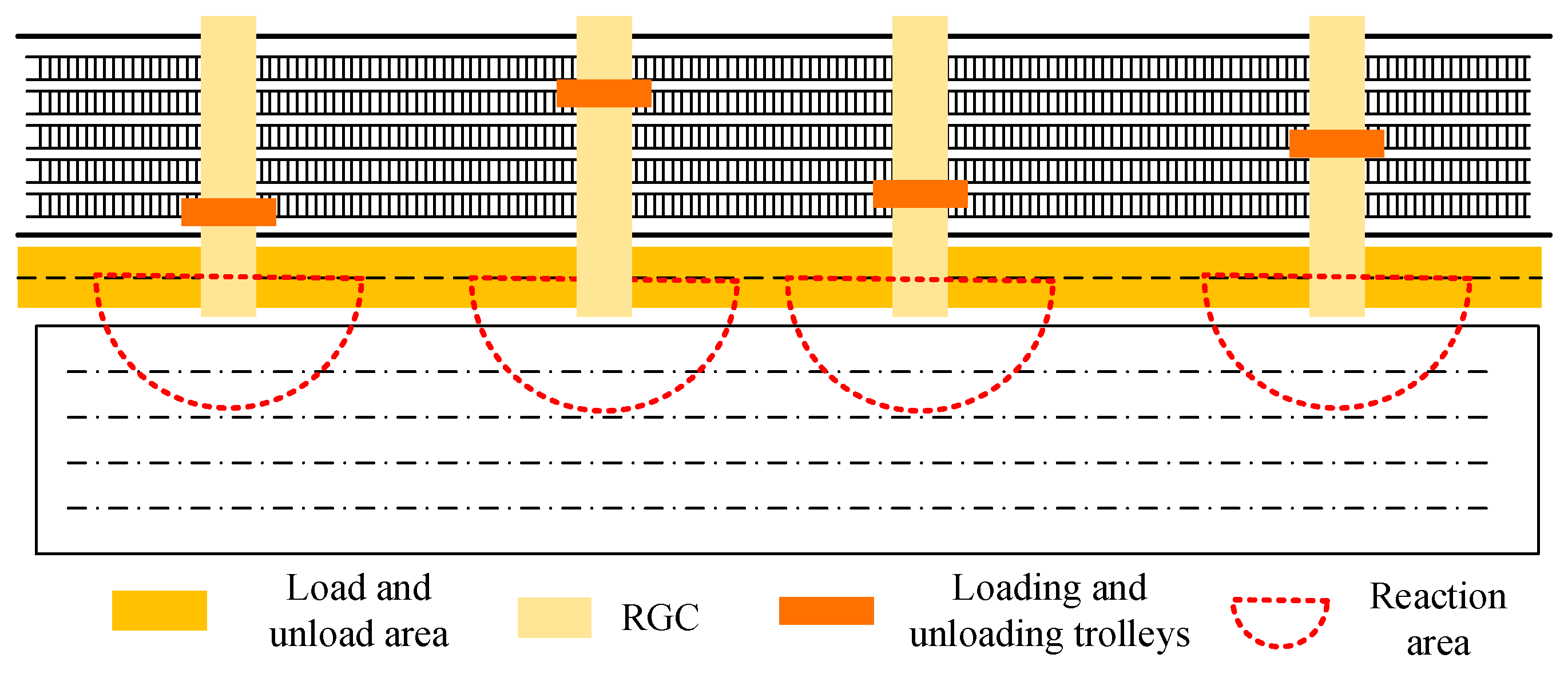
• There is a special loading and unloading channel under the RGC, which is separated from the drive channel of the IGVs, the drive channel cannot complete loading and unloading, and the IGV cannot travel more than one body distance on the loading and unloading channel to leave the loading and unloading channel;
• Each IGV has enough power, i.e., stoppages are not taken into account;
• The dimensions of all containers are standard size, and there is no situation where one IGV loads two standard containers;
• The speed change when the IGV turns is not considered.

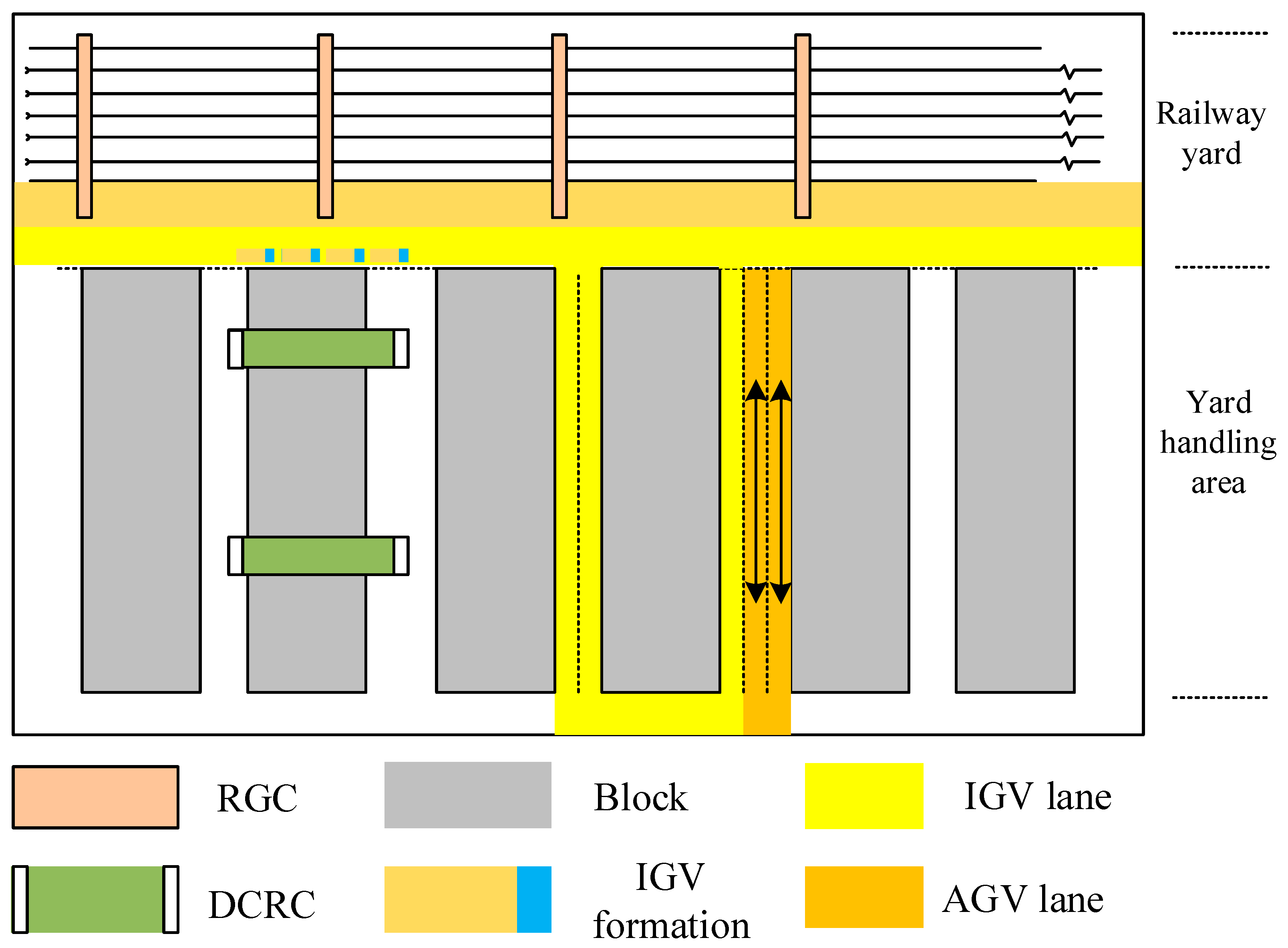
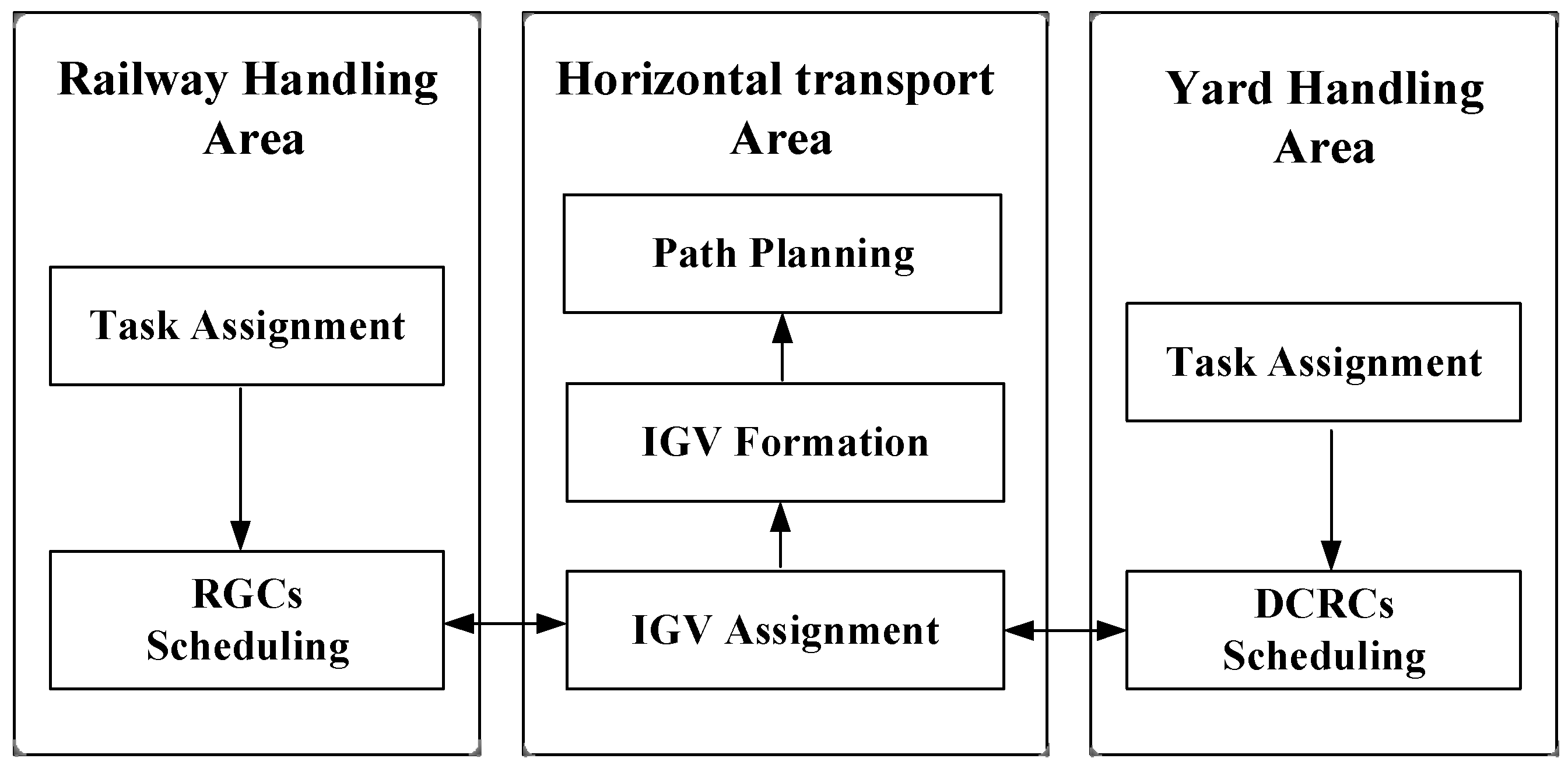
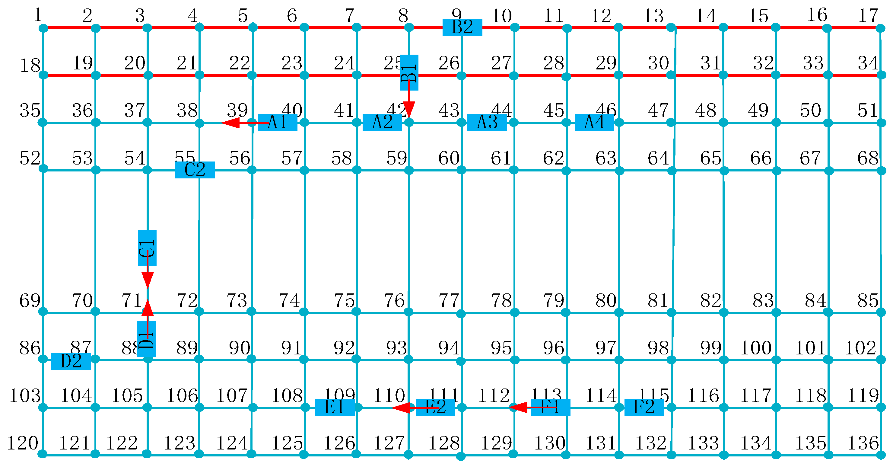
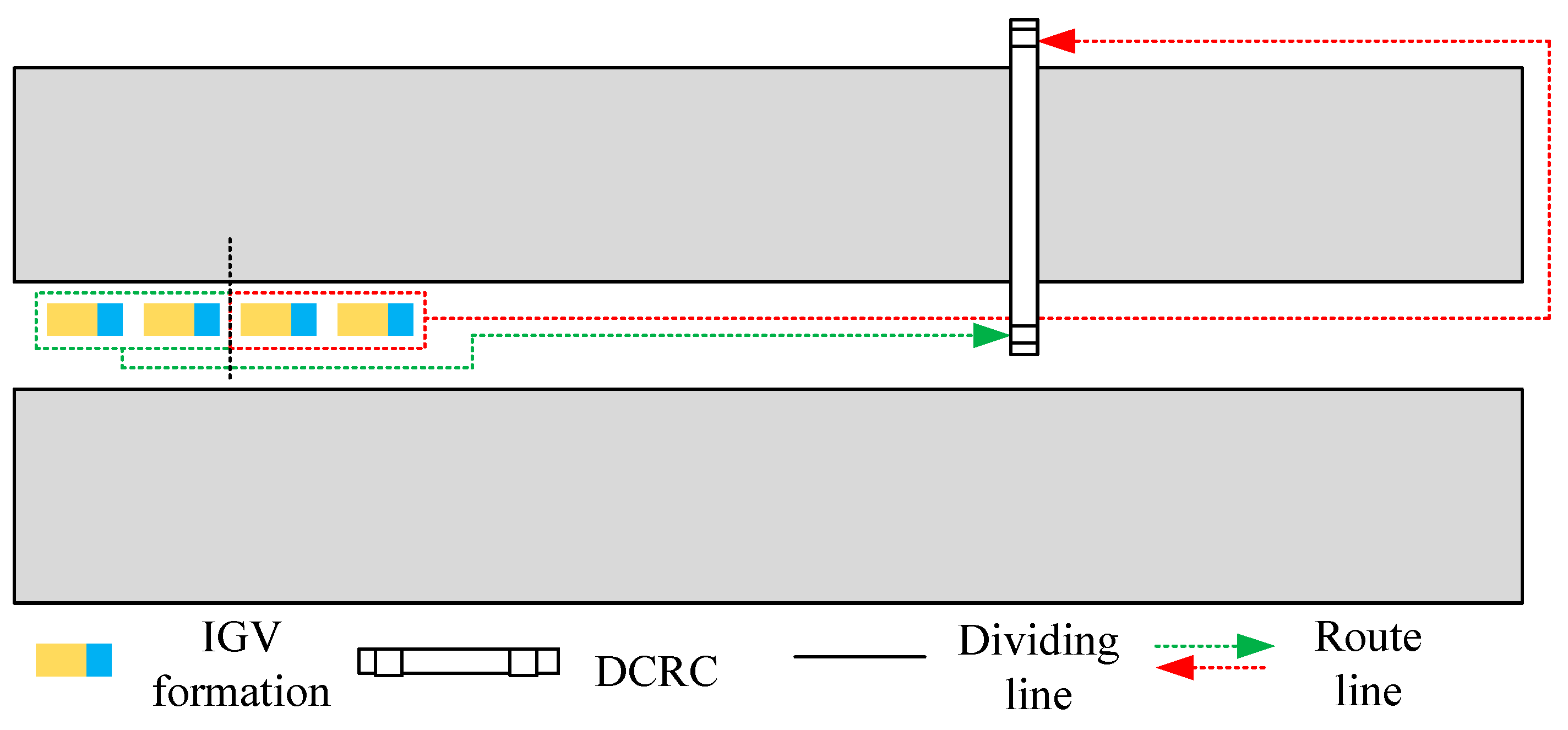
3.2. Problems Description

This paper examines the container operations between the railway yard and the yard. It focuses on multi-equipment cluster scheduling of RGCs, IGVs, and DCRCs, in order to improve the efficiency of terminal operations and shorten the loading and unloading time of trains in the port as much as possible. The problem is divided into three parts: the first is the RGC loading and unloading process; the second is the path planning process of IGVs formation; the third is the loading and unloading process of DCRCs. As shown in Figure 2, when freight trains enter the railway depot, we arrange the RGC and the corresponding block in advance. RGCs are responsible for loading and unloading containers onto IGVs; IGVs then search for the best path in the horizontal transport area and then enter the yard to interact with DCRCs to complete loading and unloading tasks. The IGVs that have completed the handover then leave the yard along the U-shaped path in the yard and reassign the IGVs to tasks. The IGVs then arrive at the railway yard loading dock and interact with the RGCs until all tasks are completed. If the container needs to be transported from the yard to the railway yard, the container transportation process is reversed.

3.3. Parameter Description

The relevant parameters of the model proposed in this paper are shown in

Table 1. Indices for the model formulation.

Indices	Definitions
$C_1$	Set of RGC
$V$	Set of IGV
$C_2$	Set of DCRC
$O_1$	Set of nodes for a railway yard
$O_2$	Set of nodes for a horizontal transport area
$O_3$	Set of nodes for a yard
$w_{p(i,j)}$	The set of distances between nodes i and nodes j on path P
$C_{N1,N2}$	A set of conflict points between paths N1 and N2 of the IGV

,

Table 2. Parameters for the model formulation.

Parameters	Definitions
$o(c)$	The initial position of the crane
$d(c)$	Destination node of crane
$o(v)$	The initial position of the IGV
$d(v)$	Destination node of crane
$l_{s1}$	Safety distance of RGC
$l_{s2}$	Safety distance for DCRC
$l_{v(i,j,t,t\prime )}^v$	Reaction distance of IGV
$l_{v(t,t\prime )}^c$	The reaction distance of the loading trolley
$l_v$	The distance of vehicles inside the IGV formation
$l_s$	Safe distance between formations
$l(i,j)$	The distance between path node i and node j
${\pi }_{i,j,t,t\prime },{\epsilon }_{i,j,t,t\prime },{\lambda }_{i,j,t,t\prime },{\mu }_{i,j,t,t\prime }$	Lagrangian multipliers associated with the vehicle flow and crane flow coupling constraint, and non-crossing constraint for crane moving, respectively.
$\omega ,\rho ,\sigma ,\xi ,\vartheta ,\phi$	Non-negative penalty parameters in ADMM associated with the vehicle flow and crane flow coupling constraint, and non-crossing constraint, respectively.

and

Table 3. Decision variables for the model formulation.

Subscripts	Definitions
Decision Variables
$x_{i,j,t,t\prime }$	The RGC is at node i at time t and t at node j
$y_{i,j,t,t\prime }$	IGV is at node i at time t and t’ at node j
$z_{i,j,t,t\prime }$	The DCRC is at node i at time t and t at node j

, respectively. Table 1 represents the parameters of a collection in the model.

3.4. Model Formulation

Automating the loading and unloading process at a terminal is a complex issue. Based on the previous analysis, this paper divides the loading and unloading process of containers between the railway yard and the yard into three parts. In the loading and unloading area of the railway station, the RGCs task is assigned, and multiple RGCs begin distributed operations. In the horizontal transport area, IGVs loaded with containers of the same container master are formed in formations and search for paths, transporting containers to the target container area. In the yard loading and unloading area, DCRCs interact with IGVs in formation to complete loading and unloading. First, each of these three job processes are modeled; then, through coupling and coordination policies, the cluster scheduling process between multiple devices is realized.

3.4.1. Loading and Unloading Models of RGCs

After the train enters the port, the RGC is arranged to be responsible for the loading and unloading of containers on the freight train. Due to the characteristics of freight trains loaded with containers, the length of each incoming freight train is long, and the RGC needs to cross multiple trains for loading and unloading. Therefore, in order to improve the loading and unloading efficiency of freight train containers, multiple RGCs are arranged at the railway station to carry out loading and unloading tasks at the same time. As shown in Figure 3, in order to improve the continuity of RGC’s work, two loading and unloading lanes are set-up in the loading and unloading area of the railway depot, and two IGVs are allowed to enter the loading and unloading area at the same time to start loading and unloading tasks. As the RGC spans multiple freight trains, the transport length of each container transported by the loading trolley becomes longer. This increases the potential for mutual waiting between the RGC and IGV. Additional time to wait can lead to a decrease in productivity efficiency. To solve this problem, the reaction distance of the loading trolley for each RGC is set. That is, when the IGV reaches the reaction area, the loading and unloading trolley begins to carry out the handling of the container, to reduce the waiting time between the RGC and IGV.

$${\displaystyle \sum _{\forall c\in C_1,\left(i,j,t,t^{\prime }\right)\in E_{c1}}{x}_{i,j,t,t^{\prime }}^c}-{\displaystyle \sum _{\forall c\in C_1,(j,i,t^{\prime },t)\in E_{c1}}{x}_{j,i,t^{\prime },t}^c=\left\{\begin{array}{c}1 i=o\left(c\right), t^{\prime }=1\hfill \\ 0 j=d\left(c\right), t^{\prime }=T,(i,j)\in O_1\hfill \\ -1 others\hfill \end{array}\right.},$$

(1)

$${\displaystyle \sum _{c\in C_1}{x}_{i,j,t,t\prime }^c}+{\displaystyle \sum _{c\prime \in C_1}{\displaystyle \sum _{(i\prime ,j\prime ,\tau ,\tau \prime )\in \varphi (i,j,t,t\prime )}{x}_{i\prime ,j\prime ,\tau ,\tau \prime }^{c\prime }\le 1}},\forall \left(i,j\right)\in O_1,$$

(2)

$$\left|{\displaystyle \sum _{c\in C_1,\left(\mathrm{i},\mathrm{j}\right)\in O_1}{x}_{i,j}^c}-{\displaystyle \sum _{c\prime \in C_1,(i,j)\in O_1}{x}_{i\prime ,j\prime }^{c\prime }}\right|\ge l_{s_1},$$

(3)

$${\displaystyle \sum _{c\in C_1}{l}_{v(t,t\prime )}^c}-{\displaystyle \sum _{v\in V}{l}_{v(i,j,t,t\prime )}^v\ge 0},\forall \left(i,j\right)\in o_2,l\in L,$$

(4)

$$x_{i,j,t,t\prime }^c\in \left\{\left.0,1\right\}\right.,$$

(5)

Equation (1) indicates the flow balance constraint during the operation of the rail gantry crane; Constraints (2) and (3) indicate the non-crossing constraints and safety distance constraints to avoid collision during the operation of the rail gantry crane, respectively; Constraint (4) indicates the unequal relationship between the reaction distance of the loading and unloading trolley and the IGV, that is, the phenomenon that the loading and unloading trolley cannot wait for the IGV to be loaded and unloaded; Equation (5) represents a binary constraint.

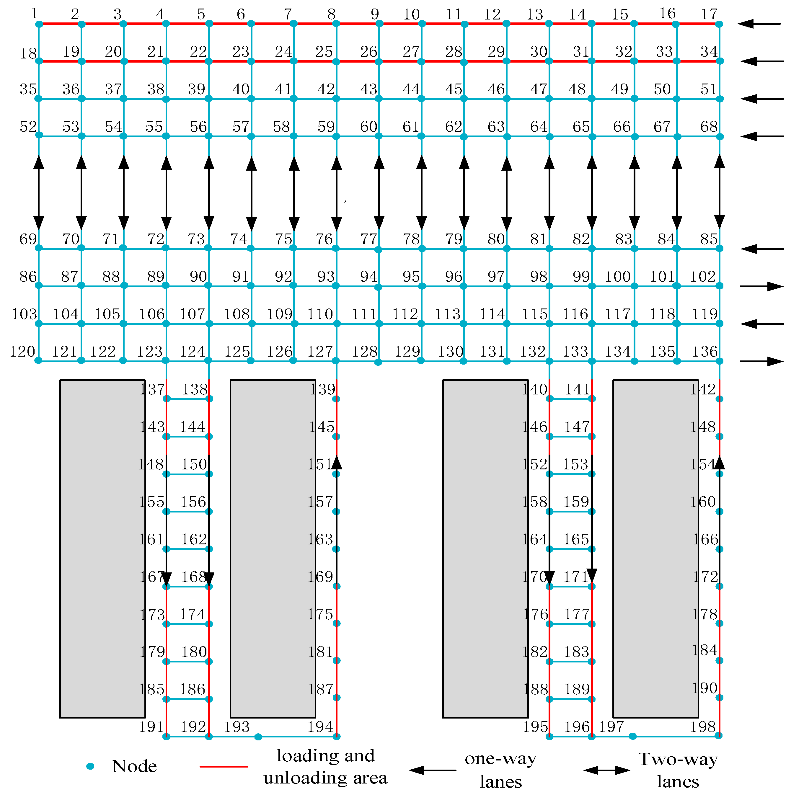
3.4.2. Conflict-Free Path Planning Model for IGVs Formations

This article sets formation rules for these IGVs going to the same box area. The number of formations is determined by the number of IGVs going to the same box area in the same time period. When the IGV is fully loaded, it is necessary to leave the loading and unloading area and reach the horizontal transport area by driving no more than one-body-length distance in the loading and unloading area. IGVs participating in their respective formations drive on different horizontal lanes, and as the horizontal lane is one-way, the vehicles driving in front of the horizontal lane form the leader car of the formation. At the same time, it is necessary to set a safe distance between vehicles in formation. The following vehicle follows the lead vehicle in a straight line or turns in the horizontal transport area.

In the horizontal transport area of the automated terminal, many buried magnetic nails determine the navigation and positioning of the IGV. These nails build a network of nodes for IGV walking paths. This paper divides the IGV into two parts in horizontal transportation: the first part is the horizontal transportation area connecting the railway production station and the yard, and the second part is the U-shaped channel transportation area inside the yard. As shown in Figure 4, there are two identical one-way lanes in the loading and unloading area of the railway yard, In the horizontal transport area, six one-way lanes are alternately arranged; node connections in the vertical direction are two-way lanes. In the yard, the horizontal nodal lanes are bidirectional, and the vertical nodes are unidirectional. In fact, a large number of magnetic nails are arranged in the pier to provide navigation and positioning of IGVs. In this paper, only the magnetic nails at key positions are considered as nodes in the IGV walking path. Figure 3 simulates a real-world magnetic nail with 198 key nodes. Among them, nodes 123, 124, 132, and 133 are the entry nodes into the yard. After completing the loading and unloading tasks in the yard, the U-shaped path is followed and the yard is exited from exit nodes 127 and 136.

First, the IGV coordinates the loading and unloading of containers with RGCs in the loading and unloading area of the railway yard. Fully loaded IGVs complete the above formation in the horizontal transport zone depending on the condition that the loaded containers belong to the same container owner. In order to prevent congestion during the transportation of formation vehicles, it is necessary to consider the length of the IGV and the safety distance between the formation vehicles. Figure 5 shows three different conflict scenarios for IGV formation transportation based on the railway yard path node network and IGV formation walking rules: the same point occupies conflict, formation reverse conflict, and pursuit conflict of different formations. Formations A and B show the conflict of occupying the same point. The A3 vehicle of Formation A also needs to pass through node 42, while the B1 vehicle of Formation B also needs to pass through node 42. Formation C and Formation D show the reverse conflict of the formation, with the vehicles of formation C1 needing to go from node 54 to node 71, and formation D1 from node 71 to node 54. Both formation E and formation F operate horizontally, and there is a pursuit conflict of formation vehicles F1 chasing formation vehicles E2.

$${\displaystyle {\sum }_{i\prime =1}^O{\displaystyle {\sum }_{j\prime =1}^O{y}_{i\prime ,j\prime ,t}^v}}=1,$$

(6)

$${\displaystyle \sum _{v\in V,(i,j,t,t^{\prime })\in E_v}{y}_{i,j,t,t\prime }^v}-{\displaystyle \sum _{v\in V,(i,j,t,t^{\prime })\in E_v}{y}_{j,i,t^{\prime },t}^v}=\left\{\begin{array}{c}1 ,i=o(v) t^{\prime }=1\hfill \\ -1 ,j=d(v) t^{\prime }=T\hfill \\ 0 others\hfill \end{array}\right.,$$

(7)

$${\displaystyle \sum _{v\in V,(i,j)\in O_1}{y}_{i,j,t,t\prime }^v}+{\displaystyle \sum _{v\prime \in V,(i\prime ,j\prime )\in O_1}{\displaystyle \sum _{(i,j,\tau ,\tau \prime )\in E_v}{y}_{i\prime ,j\prime ,\tau ,\tau \prime }^{v\prime }}}\le 1,$$

(8)

$${\displaystyle \sum _{v\in V}{y}_{i,j}^{f_v}={\displaystyle \sum _{i=1,v_i\in V}^m{y}_{i\prime ,j\prime }^{v_i}},\forall (i,j)\in O_1},$$

(9)

$$\left|{\displaystyle \sum _{f_v\in f}{y}_{i,j}^{f_v}}\right.-\left.{\displaystyle \sum _{f_{v\prime \in f}}{y}_{i\prime ,j\prime }^{f_{v\prime }}}-l_v\right|\ge l_s,$$

(10)

$$f_p={\displaystyle {\sum }_{i\prime =1}^{N\prime }{\displaystyle {\sum }_{j\prime }^{N\prime }{w}_{i\prime j\prime }\times p_{i\prime ,j\prime }^v}},$$

(11)

$$C_{(p_i,p_j)}=N_{P_i}^{\prime }\cap N_{p_j}^{\prime },$$

(12)

$${\displaystyle \sum _{i\ne j}{y}_{i,j}^{f_v}}={\displaystyle \sum _{j\ne m}{y}_{j,k}^{f_v}},\forall v\in V,$$

(13)

$${\displaystyle \sum _{f_v\in f,(i,j)\in O_3}{y}_{i,j,t,t^{\prime }}^{f_v}}-{\displaystyle \sum _{f_v\in f,(i,j)\in O_3}{y}_{j,i,t^{\prime },t}^{f_v}}=\left\{\begin{array}{c}1 ,i=o(v) t^{\prime }=1\hfill \\ -1 ,j=d(v) t^{\prime }=T\hfill \\ 0 others\hfill \end{array}\right.,$$

(14)

$${\displaystyle \sum _{v\in V}{y}_{i,j,t,t\prime }^{f_v}} \le 1,\forall \left(i,j\right)\in O_3,$$

(15)

$$f{P}_{(p_i{p}_j)}=\left|f_i^{v_i}{p}_i-\left.f_j^{v_j}{p}_j\right|\right.,$$

(16)

Constraint (6) means that any node in the horizontal transport area can only be occupied by one IGV at a time; Constraint (7) describes the flow balance constraint of IGVs when starting operations in the loading and unloading area of railway yards; Constraint (8) indicates that there is no crossing constraint between IGVs in the loading and unloading area, and it is emphasized in Equation (8) that when the loading and unloading trolley begins to move, the IGV waiting for loading and unloading can run; Constraint (9) indicates the formation of IGVs transporting containers of the same container owner; Formula (10) indicates the safety distance constraint between vehicles within the formation; Constraint (11) indicates that the length of the planned path p of the formation vehicle is the sum of all nodes on the formation FP; Constraint (12) represents collision detection for nodes. Constraint (13) indicates the traffic balance of the formation on the planned path. Constraint (14) indicates the IGV formation flow balance constraint entering the yard loading dock area. Constraint (15) indicates that there is a non-crossing constraint between formations when IGVs enter the yard to wait for loading and unloading operations; Constraint (16) indicates that different formation travel times conflict. When path conflicts occur between different formations, IGVs of different formations alternately pass through the conflict nodes. The formation that reaches the point of conflict first has a higher priority, passing the first IGV first. Due to the appearance and waiting of IGVs behind the formation, the distance between vehicles in the same formation increases. The car behind needs to accelerate and maintain a formation distance from the car in front.

$$L_{f^v}\ge L_{f^{v\prime }},$$

(17)

$${\displaystyle \sum _{}{y}_{i,t,t\prime }^{f^v}}+{\displaystyle \sum _{}{y}_{i,\tau ,\tau \prime }^{f^{v\prime }}=1},$$

(18)

$${\displaystyle \sum _{v\in f_v}{y}_{a,t_0,t_1,t_2}^v}={\displaystyle \sum _{v\prime \in f_v}{y}_{v,t_0,t_1,t_2}^{v\prime }},$$

(19)

Constraint (17) indicates the priority policy of formation vehicles at the point of conflict; Constraint (18) indicates that two conflicting formation vehicles alternately pass through the point of conflict; Equation (19) indicates the result constraint of vehicles behind the same formation catching up with vehicles in front after a conflict.

3.4.3. Loading and Unloading Models of DCRCs

Equipped with DCRCs in U-shaped terminal yards, each block can be provided with double-sided loading and unloading tasks. After the IGVs form a formation, the yard entrance enters the interior of the yard, follows the U-shaped path to the designated bay node, and interacts directly with the DCRC. The number of IGVs waiting for loading and unloading in the same bay position is more than the number of DCRCs; at this time, some IGVs are waiting for DCRC loading and unloading, which reduces efficiency. Considering the characteristics of DCRC bilateral loading and unloading, the IGV formation entering the yard is decomposed into two smaller formations, one of which reaches the target shell node and interacts directly with the DCRC; another formation arrives on the other side of the block to interact with the orbital crane. Figure 6 shows that the IGV formation is divided into two small-scale formations and the double cantilever rail crane interacts to complete loading and unloading, which realizes the function of double-side loading and unloading, and can decompose the unilateral loading and unloading pressure at the same time.

There are two entry channels on the inlet side of the yard and only one aisle on the outlet side. As shown in Figure 4, the formation entering the yard through nodes 123 and 132 can only complete unilateral loading and unloading, while the formation entering the yard through nodes 133 and 134 can reach the exit side path through the U-shaped path and still complete loading and unloading in the same box area. Therefore, in this paper, consider that the IGV formation entering the yard through node 133 or 134 automatically decomposes into two small formations: the first part of the formation first passes through the U-shaped path to the other side of the block to wait for loading and unloading, and the second part waits for loading and unloading at the target shell position of the entrance side path.

$${\displaystyle \sum _{\forall c\in C_2,(i,j,t,t^{\prime })\in E_{c2}}{z}_{i,j,t,t^{\prime }}^c}-{\displaystyle \sum _{\forall c\in C_2,(j,i,t^{\prime },t)\in E_{c2}}{z}_{j,i,t^{\prime },t}^c=\left\{\begin{array}{c}1 i=o\left(c\right), t^{\prime }=1\hfill \\ 0 j=d\left(c\right), t^{\prime }=T,(i,j)\in O_3\hfill \\ -1 others\hfill \end{array}\right.},$$

(20)

$${\displaystyle \sum _{c\in C_2}{z}_{i,j,t,t\prime }^c}+{\displaystyle \sum _{c\prime \in C_2}{\displaystyle \sum _{(i\prime ,j\prime ,\tau ,\tau \prime )\in \varphi (i,j,t,t\prime )}{z}_{i\prime ,j\prime ,\tau ,\tau \prime }^{c\prime }\le 1}},\forall \left(i,j\right)\in O_3,$$

(21)

$$\left|{\displaystyle \sum _{c\in C_2}{z}_{i,j,t,t\prime }^c}-{\displaystyle \sum _{c\prime \in C_2}{z}_{i\prime ,j\prime ,\tau ,\tau \prime }^{c\prime }-l_{f^v}}\right|\ge l_{s_2},$$

(22)

$$y_{i,j}^{f_v}=y_{i,j}^{f_{v1}}\cup y_{i,j}^{f_{v2}},$$

(23)

$${\displaystyle \sum _{}{y}_{i,j,t,t\prime }^{f_{v1}}}+{\displaystyle \sum _{}{y}_{i\prime ,j\prime ,\tau ,\tau \prime }^{f_{v2}}}=1,$$

(24)

$$z_{i,j,t,t\prime }^c\in \left\{0,1\right\},$$

(25)

$$y_{i,j,t,t\prime }^{f_v}\in \left\{0,1\right\},$$

(26)

Constraint (20) is the flow balance constraint of DCRCs; Constraint (21) indicates that there are non-crossing constraints between DCRCs; Constraint (22) indicates the safety distance constraint between rail cranes; Constraint (23) indicates that the formation entering the yard begins to divert, that is, one formation is divided into two small quantitative formations. Restraint (24) indicates that the formation performs loading and unloading tasks on both sides of the DCRC. Constraints (25) and (26) are binary representations.

3.4.4. Coupling Coordination Policies

The above three models consider the scheduling of RGCs in the loading and unloading area of railway yards, the collision-free path planning of IGV formations in the horizontal transportation direction, and the scheduling of DCRCs in the yard. These three scheduling models can be solved individually to obtain good solution quality. However, the scheduling optimization of a single scheduling model may not make the entire scheduling system optimal. This paper considers the loading and unloading tasks from the railway yard to the yard, and the scheduling process of the above three models needs to be considered at the same time. There are cranes and IGVs in the loading and unloading areas of railway yards and yards to complete loading and unloading tasks directly. To minimize container transit time, the integer programming model considering the RGC, IGV, and DCRC scheduling problem is established as follows:

Objective function:

$$\min Z={\displaystyle \sum _{v\in V}{\displaystyle \sum _{(i,j)\in O}{f}_{p(i,j)}^y}}{y}_{i,j,t,t\prime }^v,$$

(27)

Joint Constraints (1)–(4), (7)–(15), and (20)–(24):

$${\displaystyle \sum _{c\in C_1}{x}_{i,j,t,t\prime }^c}={\displaystyle \sum _{v\in V}{\displaystyle \sum _{(i,j)\in O_1}{y}_{i,j,t,t\prime }^v}},$$

(28)

$${\displaystyle \sum _{v\in f^v}{\displaystyle \sum _{(i,j)\in O_3}{y}_{i,j,t,t\prime }^v}}={\displaystyle \sum _{c\in C_2}{z}_{i,j,t,t\prime }^c},$$

(29)

where $f_{p(i,j)}^y$ is the IGV travel time cost. Constraint (28) couples RGCs flow with IGV traffic. Constraint (29) couples IGV formations and DCRCs.

4. Complex Task Decomposition and Alternating Direction Method of Multipliers

4.1. Decomposition of Complex Tasks

The loading and unloading of containers from the railway yard to the yard involves the loading and unloading of RGCs, the path planning of IGVs, and the loading and unloading process of DCRCs. Optimizing each individual model gives you better results. However, the optimization of monomers may not give the whole system optimal results. In the previous chapter, Equation (27) linked the variables of RGCs with the variables of IGVs. Similarly, Equation (28) also links the IGV formation variable with the DCRC variable. These two sets of couplings link the four variables, making the problem difficult to solve and leading to further computational challenges.

In order to reduce the complexity of various optimization problems, some scholars commonly use effective dual decomposition methods such as the Lagrange relaxation method, augmented Lagrange relaxation method, and ADMM. The Lagrangian relaxation method absorbs the constraints that cause problems in the objective function into the objective function and keeps the objective function linear. The augmented Lagrangian relaxation method introduces an additional quadratic penalty term in the objective function. In contrast to the augmented Lagrange relaxation method, ADMM can update variables sequentially block by block. Therefore, ADMM has the inherent advantages of symmetry breaking and strong convexity while maintaining a good problem decomposition structure [27].

4.1.1. The Original Model Is Dualized

Specifically, after the introduction of the Lagrange multiplier ${\pi }_{i,j,t,t\prime }$,${\epsilon }_{i,j,t,t\prime }$ and the ADMM penalty parameters $\omega$ and $\xi$, it is first necessary to dualize the coupling Constraints (27) and (28). In addition, in order to effectively solve the multi-commodity flow model of RGCs, IGVs, and DCRCs, Constraints (2), (8), (15), and (21) also dualize as an objective function, and it is necessary to introduce the Lagrange multiplier ${\lambda }_{i,j,t,t\prime }$, ${\mu }_{i,j,t,t\prime }$, ${\theta }_{i,j,t,t\prime }$, ${\varphi }_{i,j,t,t\prime }$, and ADMM penalty parameters $\rho$, $\delta$, $\vartheta$, and $\phi$. In addition, continuous and non-negative relaxation variables $s_{i,j,t,t\prime }^x\in \left[0,1\right]$, $s_{i,j,t,t\prime }^y\in \left[0,1\right]$, $s_{i,j,t,t\prime }^{f_v}\in \left[0,1\right]$, and $s_{i,j,t,t\prime }^z\in \left[0,1\right]$ need to be introduced to convert inequality Constraints (2), (8), (15), and (21) into equality constraints in order to facilitate the introduction of quadratic terms when using ADMM [18]. Therefore, the original coupling model is converted to a new model as follows.

$$\min Z={\displaystyle \sum _{v\in V}{\displaystyle \sum _{(i,j)\in O}{f}_{{}_{p(i,j)}}^y\times y_{i,j,t,t\prime }^v}}+{\displaystyle \sum _{i=1}^6{\displaystyle \sum _{j=1}^2{\Gamma }_{i,j}}},$$

(30)

where:

$${\Gamma }_{1,1}={\displaystyle \sum _{\left(i,j\right)\in O_1,c\in C_1,v\in V}\left\{{\pi }_{i,j,t,t\prime }\times \left[{\displaystyle \sum _{c\in C_1}{x}_{i,j,t,t\prime }^c}-{\displaystyle \sum _{v\in V}{\displaystyle \sum _{(i,j)\in O_1}{y}_{i,j,t,t\prime }^v}}\right]\right\}},$$

$${\Gamma }_{1,2}={\displaystyle \sum _{(i,j)\in O_1,c\in C,v\in V}\left\{\frac{\omega }{2}\times {\left[{\displaystyle \sum _{c\in C_1}{x}_{i,j,t,t\prime }^c}-{\displaystyle \sum _{v\in V}{\displaystyle \sum _{(i,j)\in O_1}{y}_{i,j,t,t\prime }^v}}\right]}^2\right\}},$$

$${\Gamma }_{2,1}={\displaystyle \sum _{(i,j)\in O_1,c\in C_1}\left\{{\lambda }_{i,j,\tau ,\tau \prime }\times \left[{\displaystyle \sum _{c\in C_1}{x}_{i,j,t,t\prime }^c}+{\displaystyle \sum _{c\prime \in C_1}{x}_{i\prime ,j\prime ,\tau ,\tau \prime }^{c\prime }-1}\right]\right\}},$$

$${\Gamma }_{2,2}={\displaystyle \sum _{(i,j)\in O_1,c\in C}\left\{\frac{\rho }{2}\times {\left[{\displaystyle \sum _{c\in C_1}{x}_{i,j,t,t\prime }^c}+{\displaystyle \sum _{c\prime \in C_1}{x}_{i\prime ,j\prime ,\tau ,\tau \prime }^{c\prime }}+s_{i,j,t,t\prime }^x-1\right]}^2\right\}},$$

$${\Gamma }_{3,1}={\displaystyle \sum _{(i,j)\in O_1,v\in V}\left\{{\mu }_{i,j,t,t\prime }\times \left[{\displaystyle \sum _{v\in V}{\displaystyle \sum _{\left(i,j\right)\in O_1}{y}_{i,j,t,t\prime }^v}}+{\displaystyle \sum _{v\prime \in V}{\displaystyle \sum _{\left(i\prime ,j\prime \right)\in O_1}{y}_{i\prime ,j\prime ,\tau ,\tau \prime }^{v\prime }-1}}\right]\right\}},$$

$${\Gamma }_{3,2}={\displaystyle \sum _{(i,j)\in O_1,v\in V}\left\{\frac{\sigma }{2}\times {\left[{\displaystyle \sum _{v\in V}{\displaystyle \sum _{\left(i,j\right)\in O_1}{y}_{i,j,t,t\prime }^v}}+{\displaystyle \sum _{v\prime \in V}{\displaystyle \sum _{\left(i\prime ,j\prime \right)\in O_1}{y}_{i\prime ,j\prime ,\tau ,\tau \prime }^{v\prime }+s_{i,j,t,t\prime }^y-1}}\right]}^2\right\}},$$

$${\Gamma }_{4,1}={\displaystyle \sum _{(i,j)\in O_3,f_v\in f}\left\{{\epsilon }_{{}_{i,j,\tau ,\tau \prime }}\times \left[{\displaystyle \sum _{v\in f_v}{\displaystyle \sum _{(i,j)\in O_3}{y}_{i,j,t,t\prime }^v}}-{\displaystyle \sum _{c\in C_2}{z}_{i,j,t,t\prime }^c}\right]\right\}},$$

$${\Gamma }_{4,2}={\displaystyle \sum _{(i,j)\in O_3,f_v\in f,c\in C_2}\left\{\frac{\xi }{2}\times {\left[{\displaystyle \sum _{v\in f_v}{\displaystyle \sum _{(i,j)\in O_3}{y}_{i,j,t,t\prime }^v}}-{\displaystyle \sum _{c\in C_2}{z}_{i,j,t,t\prime }^c}\right]}^2\right\}},$$

$${\Gamma }_{5,1}={\displaystyle \sum _{(i,j)\in O_3,v\in V,f_v\in f}\left\{{\theta }_{i,j,t,t\prime }\times \left[{\displaystyle \sum _{v\in f_v}{\displaystyle \sum _{(i,j)\in O_3}{y}_{i,j,t,t\prime }^v}} -1\right]\right\}},$$

$${\Gamma }_{5,2}={\displaystyle \sum _{(i,j)\in O_3,v\in V}\left\{\frac{\vartheta }{2}\times {\left[{\displaystyle \sum _{v\in f_v}{\displaystyle \sum _{(i,j)\in O_3}{y}_{i,j,t,t\prime }^v}}{+\mathrm{s}}_{i,j,t,t\prime }^{f_v}-1\right]}^2\right\}},$$

$${\Gamma }_{6,1}={\displaystyle \sum _{(i,j)\in O_3,c\in C_2}\left\{{\varphi }_{i,j,t,t\prime }\times \left[{\displaystyle \sum _{c\in C_2}{z}_{i,j,t,t\prime }^c}+{\displaystyle \sum _{c\prime \in C_2}{z}_{i\prime ,j\prime ,\tau ,\tau \prime }^c-1}\right]\right\}},$$

$${\Gamma }_{6,2}={\displaystyle \sum _{(i,j)\in O_3,c\in C_2}\left\{\frac{\phi }{2}\times {\left[{\displaystyle \sum _{c\in C_2}{z}_{i,j,t,t\prime }^c}+{\displaystyle \sum _{c\prime \in C_2}{z}_{i,j,\tau ,\tau \prime }^{c\prime }}+s_{i,j,t,t\prime }^z-1\right]}^2\right\}}.$$

Constraints (1), (3)–(7), (9)–(14), (16)–(20), and (22)–(26):

$${\pi }_{i,j,t,t\prime }\in R,\forall (i,j)\in O_1,$$

(31)

$${\lambda }_{i,j,t,t\prime }\ge 0,$$

(32)

$${\mu }_{i,j,t,t\prime }\ge 0,$$

(33)

$${\epsilon }_{i,j,t,t\prime }\in R,\forall (i,j)\in O_3,$$

(34)

$${\theta }_{i,j,t,t\prime }\ge 0,$$

(35)

$${\varphi }_{i,j,t,t\prime }\ge 0,$$

(36)

It can be seen that after dualizing the coupling Constraints (28) and (29) and the non-crossing Constraints (2), (8), (15), and (21), the new model can be decomposed into three subproblems $P_x$, $P_y$, and $P_z$, which correspond to the scheduling subproblem of RGCs, the IGV path subproblem, and the scheduling subproblem of DCRCs. It should be noted that as the coupling Constraints (28) and (29) are equations, the values ${\pi }_{i,j,t,t\prime }$ and ${\epsilon }_{i,j,t,t\prime }$ of the Lagrange multiplier are not constrained, while the Lagrange multiplier ${\lambda }_{i,j,t,t\prime }$,${\mu }_{i,j,t,t\prime }$, ${\theta }_{i,j,t,t\prime }$, and ${\varphi }_{i,j,t,t\prime }$ are limited to greater than or equal to 0 [27].

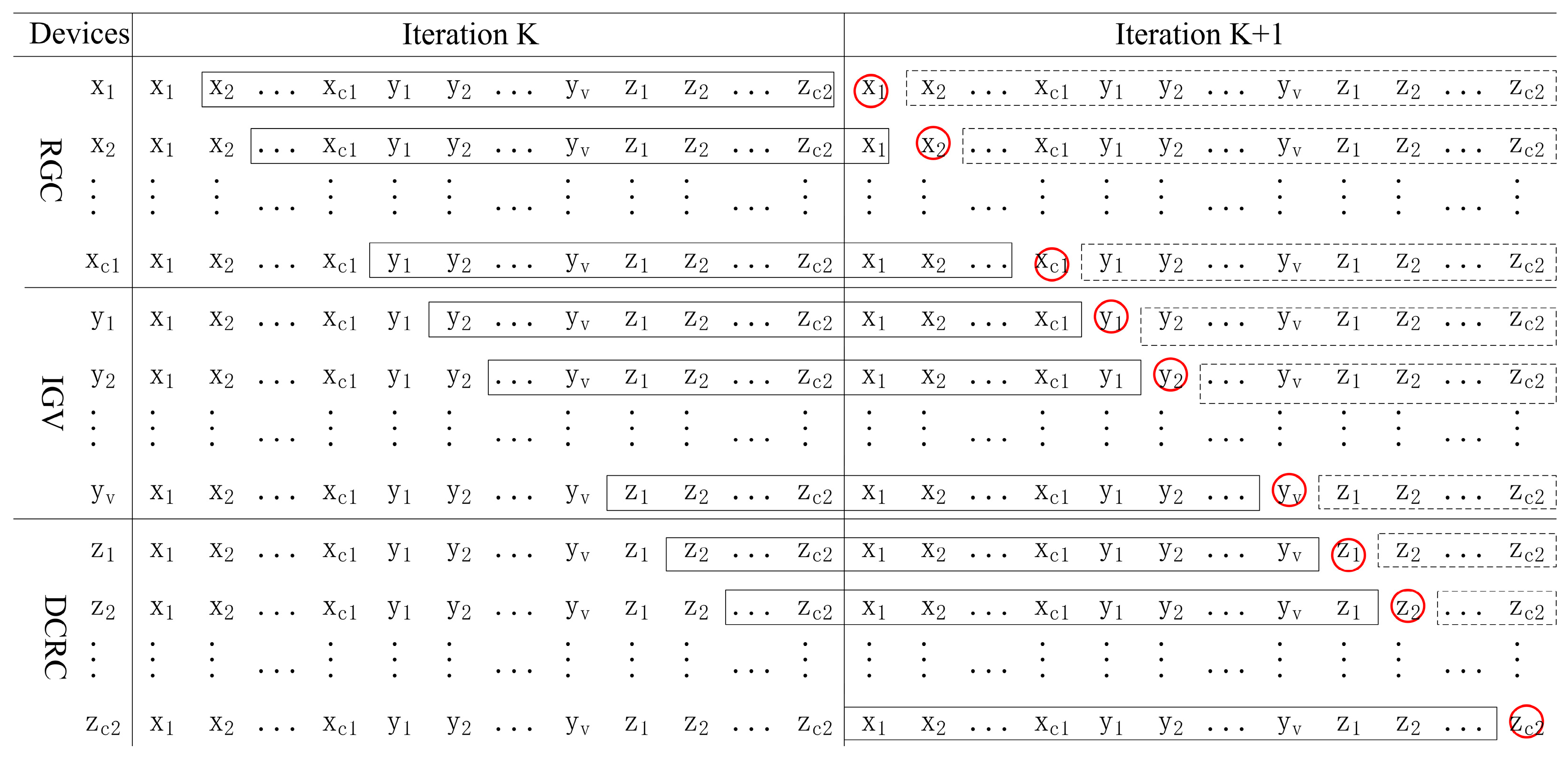
4.1.2. Gradient Descent Update Block

Note that compared to the Lagrangian relaxation method [28], the Lagrange multiplier updates the formula at the (K + 1) iteration as follows, where the updated step size is replaced by the original penalty parameter, and k represents the number of iterations.

$${\pi }_{i,j,t,t\prime }^{k+1}={\pi }_{i,j,t,t\prime }^k+\omega \left[{\displaystyle \sum _{c\in C_1}{x}_{i,j,t,t\prime }^c}-{\displaystyle \sum _{v\in V}{\displaystyle \sum _{(i,j)\in O_1}{y}_{i,j,t,t\prime }^v}}\right],$$

(37)

$${\lambda }_{i,j,t,t\prime }^{k+1}={\lambda }_{i,j,t,t\prime }^k+\rho \left[{\displaystyle \sum _{c\in C_1}{x}_{i,j,t,t\prime }^c}+{\displaystyle \sum _{c\prime \in C_1}{x}_{i,j,\tau ,\tau \prime }^{c\prime }}{s}_{i,j,t,t\prime }^x-1\right],$$

(38)

$${\mu }_{i,j,t,t\prime }^{k+1}={\mu }_{i,j,t,t\prime }^k+\sigma \left[{\displaystyle \sum _{v\in V}{\displaystyle \sum _{(i,j)\in O_1}{y}_{i,j,t,t\prime }^v}}+{\displaystyle \sum _{v\prime \in V}{\displaystyle \sum _{(i,j)\in O_1}{x}_{i,j,\tau ,\tau \prime }^{c\prime }+s_{i,j,t,t\prime }^x}}-1\right],$$

(39)

$${\epsilon }_{i,j,t,t\prime }^{k+1}={\epsilon }_{i,j,t,t\prime }^k+\xi \left[{\displaystyle \sum _{v\in f_v}{\displaystyle \sum _{(i,j)\in O3}{y}_{i,j,t,t\prime }^v}}-{\displaystyle \sum _{c\in C_2}{z}_{i,j,t,t\prime }^c}\right],$$

(40)

$${\theta }_{i,j,t,t\prime }^{k+1}={\epsilon }_{i,j,t,t\prime }^k+\vartheta \left[{\displaystyle \sum _{v\in f_v}{\displaystyle \sum _{(i,j)\in O_3}{y}_{i,j,t,t\prime }^v}}+s_{i,j,t,t\prime }^{f_v}-1\right],$$

(41)

$${\varphi }_{i,j,t,t\prime }^{k+1}={\varphi }_{i,j,t,t\prime }^k+\phi \left[{\displaystyle \sum _{c\in C_2}{z}_{i,j,t,t\prime }^c}+{\displaystyle \sum _{c\prime \in C_2}{z}_{i,j,\tau ,\tau \prime }^{c\prime }}+s_{i,j,t,t\prime }^z-1\right],$$

(42)

However, the quadratic penalty terms ${{\displaystyle [{\displaystyle \sum _{c\in C_1}{x}_{i,j,t,t\prime }^c}-{\displaystyle \sum _{v\in V}{\displaystyle \sum _{(i,j)\in O_1}{y}_{i,j,t,t\prime }^v}}]}}^2$ and ${[{\displaystyle \sum _{v\in f_v}{\displaystyle \sum _{(i,j)\in O_3}{y}_{i,j,t,t\prime }^v}}-{\displaystyle \sum _{c\in C_2}{z}_{i,j,t,t\prime }^c}]}^2$ in the objective function (30) still contain variables ${\displaystyle \sum _{c\in C_1}{x}_{i,j,t,t\prime }^c}$ and ${\displaystyle \sum _{v\in V}{\displaystyle \sum _{(i,j)\in O_1}{y}_{i,j,t,t\prime }^v}}$ and variables ${\displaystyle \sum _{v\in f_v}{\displaystyle \sum _{(i,j)\in O_3}{y}_{i,j,t,t\prime }^v}}$ and ${\displaystyle \sum _{c\in C_2}{z}_{i,j,t,t\prime }^c}$ coupled together. Therefore, it is difficult to solve subproblems $P_x$, $P_y$, and $P_z$ separately. On the other hand, if we treat each crane and each IGV as a separate module, ADMM’s rolling update scheme allows us to optimize the variables of one module, while the variables of the remaining blocks are fixed [29]. When subproblem $P_x$ is optimized, the paths of the IGV and DCRC are fixed. Therefore, it is stable for ${\displaystyle \sum _{v\in V}{\displaystyle \sum _{(i,j)\in O_1}{y}_{i,j,t,t\prime }^v}}$ and ${\displaystyle \sum _{c\in C_2}{z}_{i,j,t,t\prime }^c}$ and can be treated as constant terms $su{m}_y={\displaystyle \sum _{v\in V}{\displaystyle \sum _{(i,j)\in O_1}{y}_{i,j,t,t\prime }^v}}$ and $su{m}_z={\displaystyle \sum _{c\in C_2}{z}_{i,j,t,t\prime }^c}$, respectively. Similarly, when optimizing the $P_y$ problem, it can also be treated as a constant for ${\displaystyle \sum _{c\in C_1}{x}_{i,j,t,t\prime }^c}$ and ${\displaystyle \sum _{c\in C_2}{z}_{i,j,t,t\prime }^c}$, where $su{m}_x={\displaystyle \sum _{c\in C_1}{x}_{i,j,t,t\prime }^c}$ is set. When optimizing problem $P_z$, ${\displaystyle \sum _{c\in C_1}{x}_{i,j,t,t\prime }^c}$ and ${\displaystyle \sum _{v\in V}{\displaystyle \sum _{(i,j)\in O_1}{y}_{i,j,t,t\prime }^v}}$ can also be treated as constant terms set above. Therefore, the above problems can be broken down into specific crane sub-problems and specific IGV sub-problems.

4.1.3. Linearization of RGC Sub-Problem $P_x$

Objective function:

$$\min L_x={\displaystyle \sum _{i=1}^2{\displaystyle \sum _{j=1}^2{\Phi }_{ij}}},$$

(43)

where in:

$${\Phi }_{11}={\displaystyle \sum _{\left(i,j\right)\in O_1,c\in C_1,v\in V}\left\{{\pi }_{i,j,t,t\prime }\times {\displaystyle \sum _{c\in C_1}{x}_{i,j,t,t\prime }^c}\right\}},$$

$${\Phi }_{12}={\displaystyle \sum _{(i,j)\in O_1,c\in C,v\in V}\left\{\frac{\omega }{2}\times {\left[{\displaystyle \sum _{c\in C_1}{x}_{i,j,t,t\prime }^c}-su{m}_y\right]}^2\right\}},$$

$${\Phi }_{21}={\displaystyle \sum _{(i,j)\in O_1,c\in C_1}\left\{{\lambda }_{i,j,\tau ,\tau \prime }\times \left[{\displaystyle \sum _{c\in C_1}{x}_{i,j,t,t\prime }^c}+{\displaystyle \sum _{c\prime \in C_1}{x}_{i,j,\tau ,\tau \prime }^{c\prime }}-1\right]\right\}},$$

$${\Phi }_{22}={\displaystyle \sum _{(i,j)\in O_1,c\in C}\left\{\frac{\rho }{2}\times {\left[{\displaystyle \sum _{c\in C_1}{x}_{i,j,t,t\prime }^c}+{\displaystyle \sum _{c\prime \in C_1}{x}_{i,j,\tau ,\tau \prime }^{c\prime }}+s_{i,j,t,t\prime }^x-1\right]}^2\right\}},$$

These are Constraints (1), (3)–(5), (28), (29), and (34).

For problem $P_x$, binary variables are involved in the objective function. The second penalty term needs to be linearized first so that the block coordinate descent method can be applied to solve the subproblems of each specific vehicle [26]. As mentioned earlier, due to ADMM’s rolling update scheme, variable $x_{i,j,t,t\prime }^c$ in each update scheme is only for a specific crane, while all variables for other IGVs and DCRCs are fixed. If the rail gantry crane that currently needs to be optimized is represented by $u$, the remaining rail gantry crane belongs to $u\prime =\left\{u\prime \right\}$. We use the constant ${\mathrm{m}}_{u1}(i,j,t,t\prime )$ and its symbol $m_{u1}$ instead of the number of RGCs in the remaining set $u\prime$. As $x_{i,j,t,t\prime }^c$ is a binary number, its square is still itself. Therefore, the quadratic term in Equation (43) can be linearized directly, and the linearization result is as follows: (44) and (45).

$$\begin{array}{l}{\left[{\displaystyle \sum _{c\in C_1}{x}_{i,j,t,t\prime }^c}-su{m}_{y1}\right]}^2={\left[x_{i,j,t,t\prime }^c+m_{u1}-su{m}_{y1}\right]}^2\\ ={\left(x_{i,j,t,t\prime }^c\right)}^2+2x_{i,j,t,t\prime }^c\left(m_{u1}-su{m}_{y1}\right)+{\left(m_{u1}-su{m}_{y1}\right)}^2\\ =x_{i,j,t,t\prime }^c\left(2m_{u1}-2su{m}_{y1}+1\right)+{\left(m_{u1}-su{m}_{y1}\right)}^2\end{array},$$

(44)

$$\begin{array}{l}{\left[{\displaystyle \sum _{c\in C_1}{x}_{i,j,t,t\prime }^c}+{\displaystyle \sum _{c\prime \in C_1}{x}_{i\prime ,j\prime ,\tau ,\tau \prime }^{c\prime }}+s_{i,j,t,t\prime }^x-1\right]}^2\\ ={\left[x_{i,j,t,t\prime }^c+m_{u1}+m_{u1}+s_{i,j,t,t\prime }^x-1\right]}^2\\ ={\left(x_{i,j,t,t\prime }^c\right)}^2+2x_{i,j,t,t\prime }^c\left(2m_{u1}+s_{i,j,t,t\prime }^x-1\right)+{\left(2m_{u1}+s_{i,j,t,t\prime }^x-1\right)}^2\\ =x_{i,j,t,t\prime }^c\left(4m_{u1}+2s_{i,j,t,t\prime }^x-1\right)+{\left(2m_{u1}+s_{i,j,t,t\prime }^x-1\right)}^2\end{array},$$

(45)

Equation (45) contains the relaxation variable $s_{i,j,t,t\prime }^x$ that needs to be determined. We first consider Equation (45) as a univariate quadratic function of $L_{s_{i,j,t,t\prime }^x}$ with respect to $s_{i,j,t,t\prime }^x$ and $s_{i,j,t,t\prime }^x$ as a continuous variable, as shown in Equation (46). Optimizing the value of the variable $s_{i,j,t,t\prime }^x$ is such that $L_{s_{i,j,t,t\prime }^x}$ takes the minimum value, so when $s_{i,j,t,t\prime }^x$ is $s_{i,j,t,t\prime }^x{}^{\prime }$, the optimal solution is satisfied, and the expression $s_{i,j,t,t\prime }^x{}^{\prime }$ is shown in Equation (47). Analysis of Equation (47) shows that the theoretical value of $s_{i,j,t,t\prime }^x{}^{\prime }$ is always less than 0, and the optimal value of $s_{i,j,t,t\prime }^x$ is 0 due to the non-negative condition of the relaxation variable. The linearization of Equation (45) can be converted to (48).

$$\begin{array}{l}{L}_{s_{i,j,t,t\prime }^x}=x_{i,j,t,t\prime }^c\left(4m_{u1}+2s_{i,j,t,t\prime }^x-1\right)+{\left(2m_{u1}+s_{i,j,t,t\prime }^x-1\right)}^2\\ ={\left(s_{i,j,t,t\prime }^x\right)}^2+2\left(2m_{u1}-1+x_{i,j,t,t\prime }^c\right)s_{i,j,t,t\prime }^x+x_{i,j,t,t\prime }^c\left(4m_{u1}-1\right)+{\left(2m_{u1}-1\right)}^2\end{array},$$

(46)

$$s_{i,j,t,t\prime }^x{}^{\prime }=1-2m_{u1}-x_{i,j,t,t\prime }^c,$$

(47)

$$\begin{array}{l}{\left[{\displaystyle \sum _{c\in C_1}{x}_{i,j,t,t\prime }^c}+{\displaystyle \sum _{c\prime \in C_1}{x}_{i\prime ,j\prime ,\tau ,\tau \prime }^{c\prime }}+s_{i,j,t,t\prime }^x-1\right]}^2\\ =x_{i,j,t,t\prime }^c\left(4m_{u1}-1\right)+{\left(2m_{u1}-1\right)}^2\end{array},$$

(48)

After linearizing the two quadratic terms of Equation (42), we can generate a linearized space–time arc usage cost for each crane in subproblem $P_x$, and the model can be expressed as:

$$\min L_x^c={\displaystyle \sum _{c\in C_1}{\displaystyle \sum _{(i,j)\in O_1}{\widehat{f}}_{p(i,j)}^x}}{x}_{i,j,t,t\prime }^c+Q_x,$$

(49)

where $c_{i,j,t,t\prime }^{c1}$ is the time cost used by the RGC in the scheduling process, and $Q_x$ denotes the items irrelevant to $x_{i,j,t,t\prime }^c$.

$${\widehat{f}}_{p\left(i,j\right)}^x=\left\{\begin{array}{ccc}{f}_{p\left(i,j\right)}^x+{\pi }_{i,j,t,t\prime }+\frac{\omega }{2}\times \left(2m_{{}_{u1}}-2su{m}_{y1}+1\right)& (i,j,t,t\prime )\in E_c& \\ f_{p\left(i,j\right)}^x+{\lambda }_{i,j,t,t\prime }+\frac{\rho }{2}\times \left(4m_{u1}-1\right)& (i,j,t,t\prime )\in E_{cv}& \\ f_{p\left(i,j\right)}^x& others& \end{array}\right.$$

(50)

where $c_{i,j,t,t\prime }^{c1},$ is the time cost used by the RGC in the scheduling process, and $Q_x$ denotes the items irrelevant to $x_{i,j,t,t\prime }^c$.

4.1.4. Linearization of IGV Formation Path Sub-Problem $P_y$

Objective function:

$$\min Z={\displaystyle \sum _{v\in V}{\displaystyle \sum _{(i,j)\in O}{f}_{{}_{p(i,j)}}^y\times y_{i,j,t,t\prime }^v}}-{\Omega }_{01}+{\Omega }_{10}+{\displaystyle \sum _{i=1}^3{\displaystyle \sum _{j=1}^2{\Omega }_{i,j}}},$$

(51)

where in:

$${\Omega }_{01}={\displaystyle \sum _{\left(i,j\right)\in O_1,c\in C_1,v\in V}\left\{{\pi }_{i,j,t,t\prime }\times \left[{\displaystyle \sum _{v\in V}{\displaystyle \sum _{(i,j)\in O_1}{y}_{i,j,t,t\prime }^v}}\right]\right\}},$$

$${\Omega }_{10}={\displaystyle \sum _{(i,j)\in O_1,c\in C,v\in V}\left\{\frac{\omega }{2}\times {\left[su{m}_x-{\displaystyle \sum _{v\in V}{\displaystyle \sum _{(i,j)\in O_1}{y}_{i,j,t,t\prime }^v}}\right]}^2\right\},}$$

$${\Omega }_{11}={\displaystyle \sum _{(i,j)\in O_1,v\in V}\left\{{\mu }_{i,j,t,t\prime }\times \left[{\displaystyle \sum _{v\in V}{\displaystyle \sum _{\left(i,j\right)\in O_1}{y}_{i,j,t,t\prime }^v}}+{\displaystyle \sum _{v\prime \in V}{\displaystyle \sum _{\left(i\prime ,j\prime \right)\in O_1}{y}_{i\prime ,j\prime ,\tau ,\tau \prime }^{v\prime }-1}}\right]\right\},}$$

$${\Omega }_{12}={\displaystyle \sum _{(i,j)\in O_1,v\in V}\left\{\frac{\sigma }{2}\times {\left[{\displaystyle \sum _{v\in V}{\displaystyle \sum _{\left(i,j\right)\in O_1}{y}_{i,j,t,t\prime }^v}}+{\displaystyle \sum _{v\prime \in V}{\displaystyle \sum _{\left(i\prime ,j\prime \right)\in O_1}{y}_{i\prime ,j\prime ,\tau ,\tau \prime }^{v\prime }+s_{i,j,t,t\prime }^y-1}}\right]}^2\right\}},$$

$${\Omega }_{21}={\displaystyle \sum _{(i,j)\in O_3,f_v\in f}\left\{{\epsilon }_{{}_{i,j,\tau ,\tau \prime }}\times \left[{\displaystyle \sum _{v\in f_v}{\displaystyle \sum _{(i,j)\in O_3}{y}_{i,j,t,t\prime }^v}}-su{m}_z\right]\right\}},$$

$${\Omega }_{22}={\displaystyle \sum _{(i,j)\in O_3,f_v\in f,c\in C_2}\left\{\frac{\xi }{2}\times {\left[{\displaystyle \sum _{v\in f_v}{\displaystyle \sum _{(i,j)\in O_3}{y}_{i,j,t,t\prime }^v}}-su{m}_z\right]}^2\right\}},$$

$${\Omega }_{31}={\displaystyle \sum _{(i,j)\in O_3,v\in V,f_v\in f}\left\{{\theta }_{i,j,t,t\prime }\times \left[{\displaystyle \sum _{v\in f_v}{\displaystyle \sum _{(i,j)\in O_3}{y}_{i,j,t,t\prime }^v}} -1\right]\right\}},$$

$${\Omega }_{32}={\displaystyle \sum _{(i,j)\in O_3,v\in V}\left\{\frac{\vartheta }{2}\times {\left[{\displaystyle \sum _{v\in f_v}{\displaystyle \sum _{(i,j)\in O_3}{y}_{i,j,t,t\prime }^v}}{+\mathrm{s}}_{i,j,t,t\prime }^{f_v}-1\right]}^2\right\}},$$

These are Constraints (6), (7), (9)–(14), (16)–(19), (30), and (32)–(34).

Similar to the $P_x$ problem solution, the linearization of $P_y$ is expressed as follows:

$$\min L_y^v={\displaystyle \sum _{v\in V}{\displaystyle \sum _{(i,j)\in O_1}{\widehat{f}}_{p(i,j)}^y}}{y}_{i,j,t,t\prime }^v+Q_y,$$

(52)

4.1.5. Linearization of DCRC Sub-Problem $P_z,$

Objective function:

$$\min Z=-{\displaystyle \sum _{i=1}^2{\displaystyle \sum _{j=1}^2{\Theta }_{ij}}},$$

(53)

where in:

$${\Theta }_{11}={\displaystyle \sum _{(i,j)\in O_3,f_v\in f}\left\{{\epsilon }_{{}_{i,j,\tau ,\tau \prime }}\times \left[{\displaystyle \sum _{c\in C_2}{z}_{i,j,t,t\prime }^c}\right]\right\}},$$

$${\Theta }_{12}={\displaystyle \sum _{(i,j)\in O_3,f_v\in f,c\in C_2}\left\{\frac{\xi }{2}\times {\left[su{m}_y-{\displaystyle \sum _{c\in C_2}{z}_{i,j,t,t\prime }^c}\right]}^2\right\}},$$

$${\Theta }_{21}={\displaystyle \sum _{(i,j)\in O_3,c\in C_2}\left\{{\varphi }_{i,j,t,t\prime }\times \left[{\displaystyle \sum _{c\in C_2}{z}_{i,j,t,t\prime }^c}+{\displaystyle \sum _{c\prime \in C_2}{z}_{i\prime ,j\prime ,\tau ,\tau \prime }^c-1}\right]\right\}},$$

$${\Theta }_{22}={\displaystyle \sum _{(i,j)\in O_3,c\in C_2}\left\{\frac{\phi }{2}\times {\left[{\displaystyle \sum _{c\in C_2}{z}_{i,j,t,t\prime }^c}+{\displaystyle \sum _{c\prime \in C_2}{z}_{i,j,\tau ,\tau \prime }^{c\prime }}+s_{i,j,t,t\prime }^z-1\right]}^2\right\}},$$

These are Constraints (20), (22)–(26), (33), and (35).

Similar to the previous processing method, after linearizing the objective function, it can be simplified to:

$$\min L_z^c={\displaystyle \sum _{c\in C_2}{\displaystyle \sum _{(i,j)\in O_3}{\widehat{f}}_{p(i,j)}^z}}{z}_{i,j,t,t\prime }^c+Q_z,$$

(54)

4.1.6. Evolution Steps

In order to further elaborate the entire ADMM framework, the key steps are explained as follows.

Step 1: Considering the non-crossing constraint of the loading and unloading process and the hard-edge constraint of flow balancing, the objective function of the original model is dualized, which is detailed in Section 4.1.1;

Step 2: The objective function optimization process of duality is conducted by gradient descent, and the gradient descent update block is designed in Section 4.1.2;

Step 3: Linearization of binary variables include non-negative relaxation variables, which is detailed in Section 4.1.3.

Step 4: Refer to the $P_x$ subproblem to complete the process of linearization of the $P_y$ subproblem, which is detailed in Section 4.1.4;

Step 5: Refer to the $P_x$ subproblem to complete the process of linearization of the $P_z$ subproblem, which is detailed in Section 4.1.5.

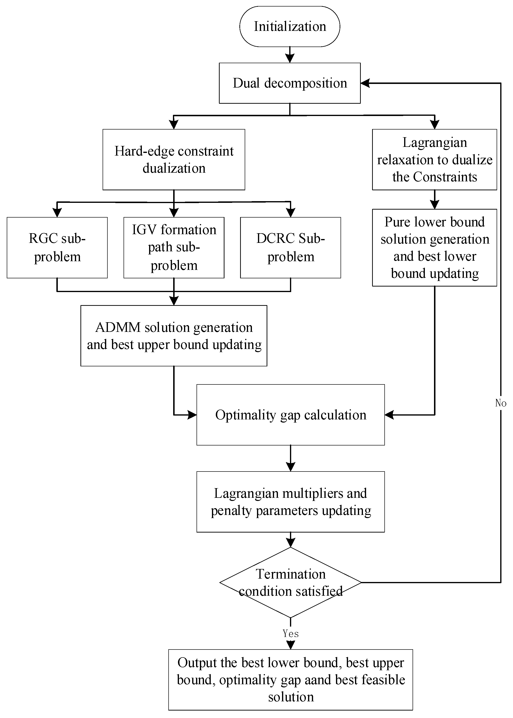
4.2. Process of ADMM-Based Solutions

The ADMM-based solution framework is shown in Figure 7. On the basis of this framework, the solution process of ADMM is used to solve the problem.

The rolling update scheme for ADMM is shown in Figure 8, where each row represents the least-cost path update for each device. Devices surrounded by red circles in each row indicate that they will be updated at the K + 1st iteration, devices surrounded by a solid matrix represent temporary fixed agents, and devices surrounded by dotted rectangles represent agents that are to be optimized at the K + 1st iteration. The node usage cost for each device is updated based on the spatiotemporal path of the fixed agent in each internal iteration.

5. Numerical Experiments

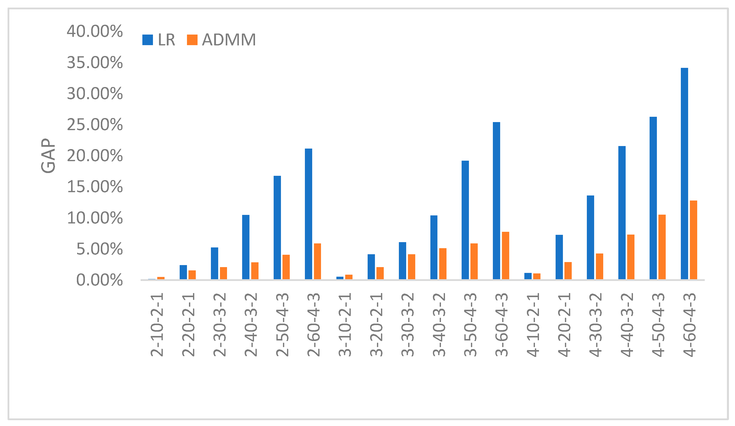
5.1. Solve the Result

In this section, we set-up 18 sets of numerical experiments for different scenarios. Considering the need to verify the effectiveness of the model and algorithm, we focus on testing the proposed algorithm and model from the perspective of optimization and efficiency. At the same time, we compare with the standard Lagrange relaxation (LR) method. The standard Lagrangian dual problem is to cut the boundary of the feasible domain and generate a feasible solution to the original problem by the original heuristic.

In the experiment, the number of IGVs is set to 10 to 60 and the number of RGCs is set to 2 to 4. Supposing the container is unloaded to a specific block, each block is equipped with a DCRC quantity of 2 to 4. In the loading and unloading area of the railway depot, the reaction distance of the loading trolley is set from 4 to 20 m. The average time cost of RGC loading and unloading operations is set at 6 to 8 time units [21]. In the yard, the time for the crane to deliver the container to the designated storage point or place the container from the storage point to the IGV obeys an even distribution of (30, 50). The spacing of containers in the yard follows an even distribution of (1, 20) [30]. The horizontal transport area is 420 m long and 180 m wide, the length of the IGV is set to 15 m, and the safety distance between the IGVs is set to 5 m. The operating speed of the IGV is set to 5 m/s. The designed ADMM is compared to the standard LR, and the numerical comparison results of the LR and ADMM algorithms are shown in

Table 4. Comparison of experimental data of LR and ADMM.

Scenario	GCs-AGVs-YCs-Blocks	LR				ADMM
		Lower Bound	Upper Bound	Iterations	CPU Time	Lower Bound	Upper Bound	Iterations	CPU Time
1	2-10-2-1	127.2	127.4	12	0.619	126.7	127.3	17	0.716
2	2-20-2-1	256.5	262.7	23	1.167	258.4	262.5	27	1.271
3	2-30-3-2	364.1	384.2	29	5.013	376	383.9	34	5.737
4	2-40-3-2	455.7	509.1	45	13.223	495.6	510.1	39	13.989
5	2-50-4-3	560.6	673.6	92	18.947	645.9	673.2	48	24.135
6	2-60-4-3	637.2	808	118	39.462	759.9	807.3	61	35.738
7	3-10-2-1	128.2	128.9	17	0.883	127.7	128.8	17	0.977
8	3-20-2-1	262	273.3	29	0.916	267.4	273.1	23	1.218
9	3-30-3-2	356.4	379.4	43	4.246	363.9	379.7	26	3.224
10	3-40-3-2	472.4	527.1	77	6.180	499.5	526.4	35	6.027
11	3-50-4-3	532.4	658.8	104	14.227	621.4	660.3	44	9.917
12	3-60-4-3	614.5	823.7	147	26.192	761.2	825.2	61	23.187
13	4-10-2-1	129.7	131.2	22	0.993	129	130.4	25	1.012
14	4-20-2-1	256.9	277	35	1.473	268.4	276.3	31	1.251
15	4-30-3-2	340.9	394.5	58	1.968	377.4	394.2	33	1.327
16	4-40-3-2	406.9	518.7	96	4.285	480.6	518.5	41	3.371
17	4-50-4-3	502.2	681.1	133	10.932	609.5	680.9	47	6.293
18	4-60-4-3	538.2	817.2	178	19.141	714.9	819.6	62	15.847

and Figure 9 below.

Analysis of the data in Table 2 and Figure 9 yields the following conclusions:

Table 2 and Figure 9 show that both methods have good convergence for solving problems. When scheduling a small number of devices, LR solving requires fewer iterations than ADMM does, such as scenarios 1, 2, 3, and 13. At the same time, the CPU runtime during LR solving is also lower than the running time of ADMM, such as scenarios 1, 2, 7, 8, and 13. Conversely, when scheduling a large number of devices, ADMM solutions take precedence over LR for CPU runtime and iteration times. The reason to explain this phenomenon is that compared with the ADMM algorithm, LR divides the feasible domain and solves the feasible solution through the original heuristic, without the need for the step of minimizing the widening of the Lagrangians, thereby reducing the running time and the number of iterations. For the quality analysis of the solution, scenario 1 and scenario 7 involve fewer scheduling devices, and the gap value of the solution solved by LR is lower than the value obtained by ADMM. when the number of devices participating in scheduling increases, the gap of the solution solved by ADMM is significantly lower than the gap value solved by LR, that is, the convergence of the solution solved by ADMM is better than that of the solution solved by LR. This can be explained by the fact that when there are too many pieces of scheduling equipment and the working range of the crane is flexible, the augmented Lagrangian increment in the ADMM algorithm limits the search space of the feasible solution, so the quality of the solution solved by ADMM is better than that of LR.

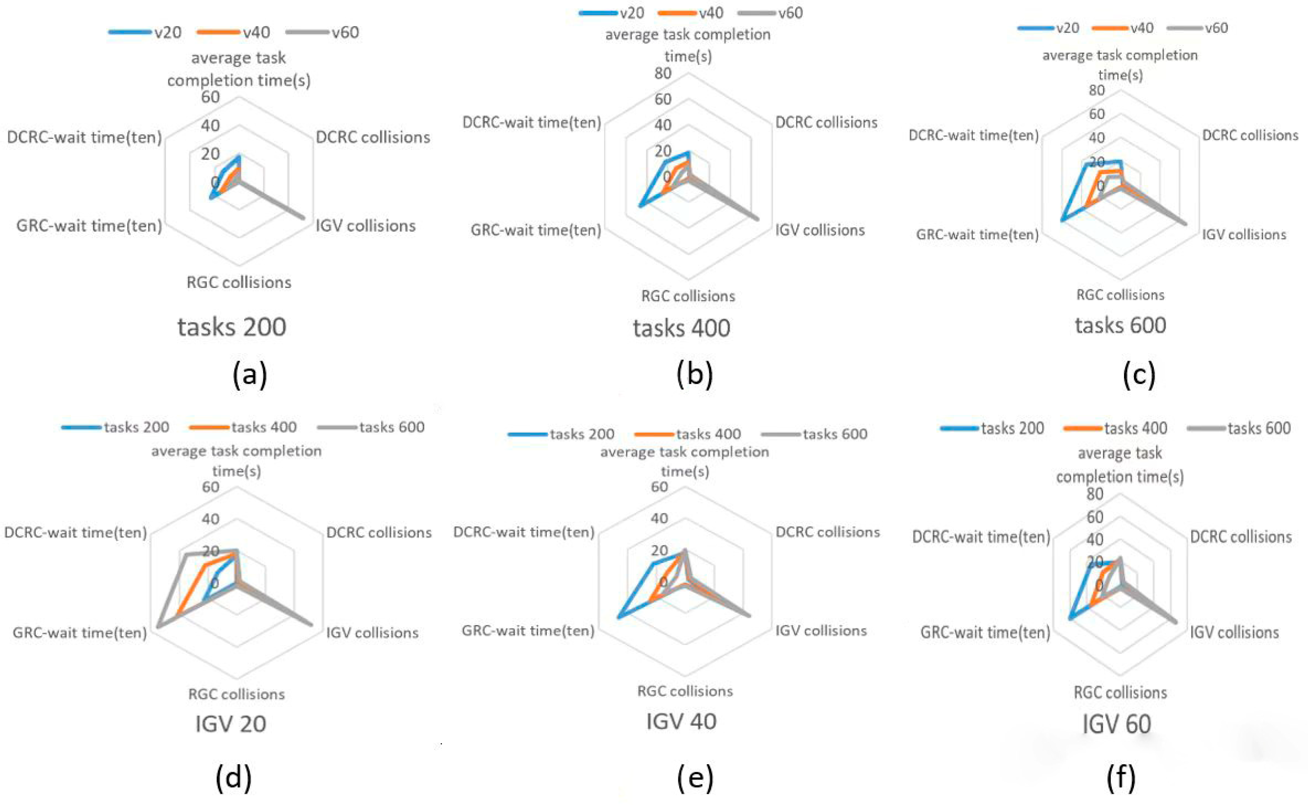
5.2. Sensitivity Analysis

In order to verify the effectiveness of the model, the allocation and scheduling results of IGVs need to be quantitatively analyzed. In the work of Li et al. (2020) [31], the number of completed tasks, total travel distance, average driving distance, and number of starts and stops were used as measurement parameters for AGV performance. The number of tasks and the number of IGVs participating in scheduling will affect the operation efficiency of the whole system, and an evaluation index system is established based on the characteristics of this problem. Sensitivity analysis of these two key factors is performed through six indicators. The six indicators are: average task completion time, DCRC collisions, IGV collisions, RGC collisions, RGC wait time, and DCRC wait time. The results of 400 tasks are shown in

Table 5. Operation efficiency evaluation indexes of 50 tasks.

Number of IGV	Average Task Completion Time (s)	DCRC Collisions	IGV Collisions	RGC Collisions	GRC Wait Time (s)	DCRC Wait Time (s)
20	48	0	0	0	17	5
30	27	0	3	0	12	0
40	18	0	11	0	5	0
50	14	0	34	0	0	0
60	11	1	61	0	0	0

, Figure 10a–c show the effect of the change in IGV quantity on the task, and Figure 10d–f show the effect of the change in task volume on the configuration of the IGV.

The following conclusions can be summarized from Figure 10:

• In the model formulation, RGCs and DCRCs are less affected by the number of tasks and the number of IGVs. This is explained by the fact that it is necessary to consider crane non-crossing constraints and safety distances in model designation.
• The waiting time of cranes is less affected by the change in the number of tasks and more affected by the number of IGVs. This shows that the IGV travel distance in the U-shaped terminal becomes longer, resulting in a waiting time gap for the crane, and increasing the number of IGVs can improve the continuous work of the crane.

The number of IGV conflicts increases with the number of tasks, and the number of IGVs is less sensitive. The main reason is that in the transshipment of containers between railway yards and yards, the average task completion time varies little, and the total task completion time is positively correlated with the task volume. The formation transportation of IGVs simplifies the transportation rules of IGVs, increases the utilization rate of transportation routes, and reduces obstacles for vehicles on the routes.

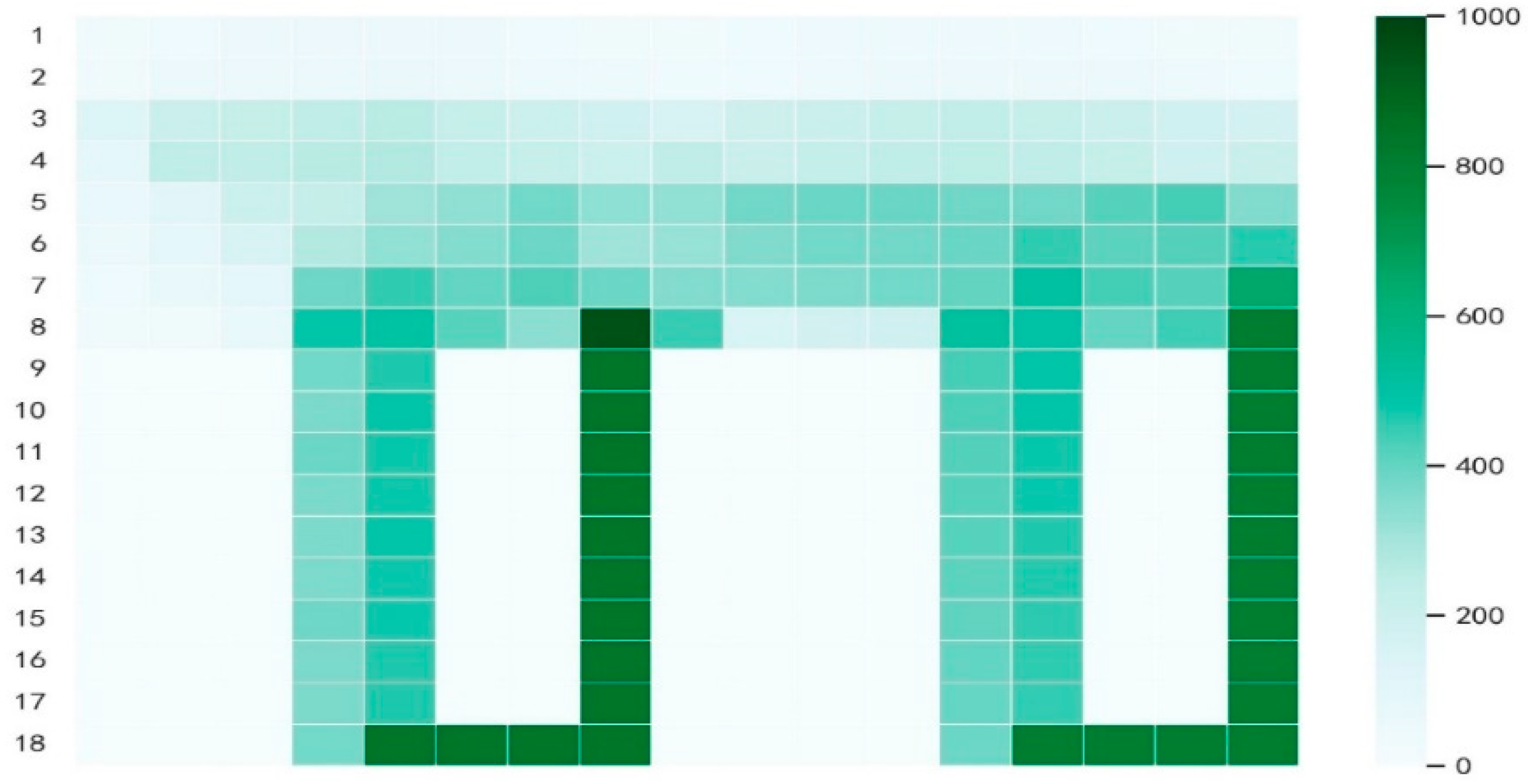
5.3. Path Experiment of IGV Formations

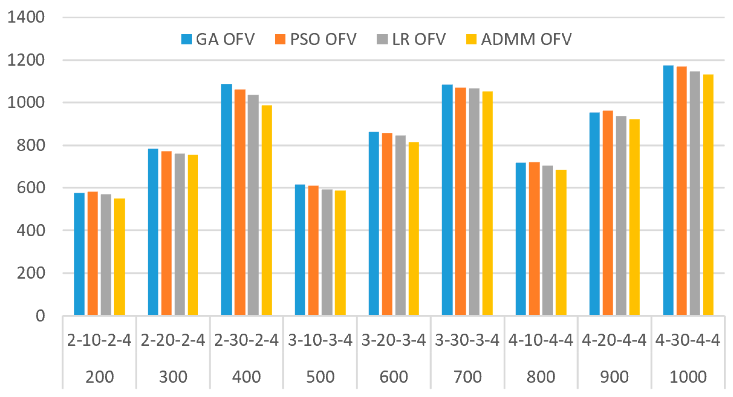
This paper considers the scheduling problem of cranes in flexible working areas, and avoids conflicts between cranes running on the same track with non-crossing constraints and crane safety distances. When flexible work areas are adopted, the workload of different cranes can be better balanced by cooperation compared to fixed work areas [30]. At the same time, the waiting time of unmanned vehicles will be reduced accordingly. The explanation for this phenomenon is that in the ADMM-based approach, the goal of crane-specific subproblems is to find a space–time least-cost path for each crane [27]. Based on the research scenario of the model in this paper, Figure 10 shows the heat map display of the IGV formation operation area in scenario 9. In a heatmap, each grid is a square centered on a path node. The shade of the grid color depends on the number of times the device is accessed, and the darker the grid color of the heatmap, the higher the number of times it has been accessed. The number of visits to the magnetic peg on the horizontal transportation area path is recorded, and a heat map of IGV formations on a horizontal path is obtained as seen in Figure 10.

From the heat map analysis of Figure 11, it can be seen that: On the U-shaped path of the yard, IGVs are visited significantly more frequently than in horizontal transport areas. The explanation for this phenomenon is that the containers are transported in IGV formations, and the loading and unloading tasks of the containers are assigned to the U-shaped path of the yard. On U-shaped path nodes, the path nodes on the exit side are accessed significantly more times than other nodes. This is due to the layout process of the yard; in the adjacent box area, there are two paths into the yard, there is only one outlet in the yard, and the IGV to complete loading and unloading needs to go through the exit path. This causes the path node on the egress side to visit more times. At the same time, the path node is accessed more frequently, which is easy to make the node more prone to conflicts with the same point occupancy. In the U-shaped terminal yard area, setting IGV formation rules can effectively avoid path conflicts.

5.4. Discussion

This paper studies the multi-equipment cluster scheduling, which is benificial to improving the collaborative processing and continuity of terminal equipment, and improve the efficiency of automated terminal and sea–rail combined transportation. However, most studies on multi-device scheduling only consider the coordination between devices [18,19,21,22,23,26] or additionally consider other goals as constraints [20,24,25]. More scholars are building mixed-integer programming models, and heuristics are mentioned more when solving models [21,22,25,26] by comparing genetic algorithms (GA) [21], particle swarm optimization (PSO) algorithms [26], and LR to verify the ability of ADMM algorithms to solve large problems. The volume of tasks for setting up containers varies from 200 to 1000. The experimental results are shown in

Table 6. OFV calculated by GA, PSO, LR, and ADMM.

Containers	RGC-IGV-DCRC-Blocks	GA	PSO	LR	ADMM
		OFV	OFV	OFV	OFV
200	2-10-2-4	577	583	569	550
300	2-20-2-4	782	773	761	755
400	2-30-2-4	1087	1061	1036	988
500	3-10-3-4	617	610	594	587
600	3-20-3-4	862	858	845	814
700	3-30-3-4	1083	1071	1068	1052
800	4-10-4-4	719	721	705	683
900	4-20-4-4	954	961	937	921
1000	4-30-4-4	1175	1169	1147	1132

.

Figure 12 shows that objective function value (OFV) becomes larger as more tasks increase. At the same time, as the number of dispatching devices increases, OFV becomes larger. Under the same conditions, the OFV calculated by ADMM is smaller than those of other algorithms. This further shows that ADMM has better performance in computing large tasks.

6. Conclusions

This paper studies the multi-equipment cluster scheduling between yards and railway depots in U-shaped terminal layouts. Considering that RGCs, IGVs, and DCRCs are characterized bygrouping operations, a mixed-integer programming model is established to minimize the container transit time. Considering non-crossing constraints and safe distance constraints as complex interactions between terminal equipments, an ADMM-based framework is proposed. Dock cluster scheduling problems is decomposed into sub-problems of specific RGCs, IGVs, and DCRCs, and the time costs were iteratively adjusted to improve the quality of the solution. In addition, we carried out a large number of numerical experiments as well as sensitivity analysis of the model and the heatmap display of IGV formations traveling on a horizontal path to test the effectiveness of the model and algorithm. Compared with common heuristic algorithms, the proposed model and algorithm can significantly improve the scheduling efficiency. Therefore, this study on multi-equipment cluster scheduling is conducive to improve the collaborative handling and continuous work of terminal equipment, and improving the efficiency of automated terminal and sea–rail intermodal transport. The automated terminal is a complete scheduling system, and managers should pay attention to consider multi-device cluster scheduling. The ADMM framework can realize the problem decomposition of complex scheduling models, and simplify the solution of the problems.

Multimodal transport is an important development direction for future terminals. The railway enters the port, connecting the terminal and the railway. Research on scheduling between terminal yards and railways will reduce the congestion of yard inventory. At the same time, it reduces transportation costs and relieves the pressure of single transportation at the terminal. However, multimodal transport at automated terminals should include not only depots to railway depots, but also cargo ships to railway yards. In future studies, multi-equipment scheduling between the coastal side of the U-shaped automated terminal and the railway should also be considered. At the same time, the study of real railway port scheduling problems will be more complex and involve more scheduling equipment (including forklifts, ships, etc.). Future research should consider more collaboration between devices to maximize the efficiency of the overall system.

References

1. Sun, Z.W. The world’s First! Zhenhua Heavy Industry Releases New Technology for Container Terminal Loading and Unloading, China Water Transport Network 2019. Available online: http://app.zgsyb.com/news.html?aid=530549 (accessed on 10 December 2022.).
2. Beibu Gulf Port. Qinzhou Port Automated Container Terminal Completed Renovation. 2021. Available online: https://www.bbwport.cn/a/xinwenzixun/gongsixinwen/938.html (accessed on 10 December 2022.).
3. Wu, Y.; Li, W.; Petering, M.E.H.; Goh, M.; de Souza, R. Scheduling multiple yard cranes with crane interference and safety distance requirement. Transp. Sci. 2015, 49, 990–1005. [Google Scholar] [CrossRef] [Green Version]
4. Gharehgozli, A.H.; Vernooij, F.G.; Zaerpour, N. A simulation study of the performance of twin automated stacking cranes at a seaport container terminal. Eur. J. Oper. Res. 2017, 261, 108–128. [Google Scholar] [CrossRef] [Green Version]
5. Nossack, J.; Briskorn, D.; Pesch, E. Container dispatching and conflict-free yard crane routing in an automated container terminal. Transp. Sci. 2018, 52, 1059–1076. [Google Scholar] [CrossRef]
6. Galle, V.; Barnhart, C.; Jaillet, P. Yard crane scheduling for container storage, retrieval, and relocation. Eur. J. Oper. Res. 2018, 271, 288–316. [Google Scholar] [CrossRef]
7. He, J.; Tan, C.; Zhang, Y. Yard crane scheduling problem in a container terminal considering risk caused by uncertainty. Adv. Eng. Inform. 2019, 39, 14–24. [Google Scholar] [CrossRef]
8. Guo, P.; Cheng, W.; Wang, Y.; Boysen, N. Gantry crane scheduling in intermodal rail-road container terminals. Int. J. Prod. Res. 2018, 56, 5419–5436. [Google Scholar] [CrossRef]
9. Lei, D.; Zhang, P.; Zhang, Y.; Xia, Y.; Zhao, S. Research on optimization of multi stage yard crane scheduling based on genetic algorithm. J. Ambient Intell. Humaniz. Comput. 2020, 11, 483–494. [Google Scholar] [CrossRef]
10. Stephan, K.; Boysen, N. Crane scheduling in railway yards: An analysis of computational complexity. J. Sched. 2017, 20, 507–526. [Google Scholar] [CrossRef]
11. Li, W.; Du, S.; Zhong, L.; He, L. Multiobjective Scheduling for Cooperative Operation of Multiple Gantry Cranes in Railway Area of Container Terminal. IEEE Access 2022, 10, 46772–46781. [Google Scholar] [CrossRef]
12. Chen, S.; Zeng, Q. Carbon-efficient scheduling problem of electric rubber-tyred gantry cranes in a container terminal. Eng. Optim. 2022, 54, 2034–2052. [Google Scholar] [CrossRef]
13. Hu, H.; Yang, X.; Xiao, S.; Wang, F. Anti-conflict AGV path planning in automated container terminals based on multi-agent reinforcement learning. Int. J. Prod. Res. 2023, 61, 1–16. [Google Scholar] [CrossRef]
14. Guo, K.; Zhu, J.; Shen, L. An improved acceleration method based on multi-agent system for AGVs conflict-free path planning in automated terminals. IEEE Access 2020, 9, 3326–3338. [Google Scholar] [CrossRef]
15. Yang, Y.; Zhong, M.; Dessouky, Y.; Postolache, O. An integrated scheduling method for AGV routing in automated container terminals. Comput. Ind. Eng. 2018, 126, 482–493. [Google Scholar] [CrossRef]
16. Miyamoto, T.; Inoue, K. Local and random searches for dispatch and conflict-free routing problem of capacitated AGV systems. Comput. Ind. Eng. 2016, 91, 1–9. [Google Scholar] [CrossRef]
17. Roy, D.; Gupta, A.; De Koster, R.B.M. A non-linear traffic flow-based queuing model to estimate container terminal throughput with AGVs. Int. J. Prod. Res. 2016, 54, 472–493. [Google Scholar] [CrossRef]
18. He, J.; Huang, Y.; Yan, W.; Wang, S. Integrated internal truck, yard crane and quay crane scheduling in a container terminal considering energy consumption. Expert Syst. Appl. 2015, 42, 2464–2487. [Google Scholar] [CrossRef]
19. Zeng, Q.; Yang, Z. Integrating simulation and optimization to schedule loading operations in container terminals. Comput. Oper. Res. 2009, 36, 1935–1944. [Google Scholar] [CrossRef]
20. Yan, B.; Jin, J.G.; Zhu, X.; Lee, D.-H.; Wang, L.; Wang, H. Integrated planning of train schedule template and container transshipment operation in seaport railway terminals. Transp. Res. Part E Logist. Transp. Rev. 2020, 142, 102061. [Google Scholar] [CrossRef]
21. Yan, B.; Zhu, X.; Wang, L.; Chang, Y. Integrated scheduling of rail-mounted gantry cranes, internal trucks and reach stackers in railway operation area of container terminal. Transp. Res. Rec. 2018, 2672, 47–58. [Google Scholar] [CrossRef]
22. Pratap, S.; Zhang, M.; Shen, C.; Huang, G.Q. A multi-objective approach to analyse the effect of fuel consumption on ship routing and scheduling problem. Int. J. Shipp. Transp. Logist. 2019, 11, 161–175. [Google Scholar] [CrossRef]
23. Kenan, N.; Jebali, A.; Diabat, A. The integrated quay crane assignment and scheduling problems with carbon emissions considerations. Comput. Ind. Eng. 2022, 165, 107734. [Google Scholar] [CrossRef]
24. Yin, Y.Q.; Zhong, M.; Wen, X.; Ge, Y.E. Scheduling quay cranes and shuttle vehicles simultaneously with limited apron buffer capacity. Comput. Oper. Res. 2023, 151, 106096. [Google Scholar] [CrossRef]
25. Hsu, H.P.; Wang, C.N.; Fu, H.P.; Dang, T.T. Joint scheduling of yard crane, yard truck, and quay crane for container terminal considering vessel stowage plan: An integrated simulation-based optimization approach. Mathematics 2021, 9, 2236. [Google Scholar] [CrossRef]
26. Li, J.; Yang, J.; Xu, B.; Yang, Y.; Wen, F.; Song, H. Hybrid scheduling for multi-equipment at U-shape trafficked automated terminal based on chaos particle swarm optimization. J. Mar. Sci. Eng. 2021, 9, 1080. [Google Scholar] [CrossRef]
27. Chen, X.; He, S.; Zhang, Y.; Tong, L.; Shang, P.; Zhou, X. Yard crane and AGV scheduling in automated container terminal: A multi-robot task allocation framework. Transp. Res. Part C Emerg. Technol. 2020, 114, 241–271. [Google Scholar] [CrossRef]
28. Mahmoudi, M.; Zhou, X. Finding optimal solutions for vehicle routing problem with pickup and delivery services with time windows: A dynamic programming approach based on state–space–time network representations. Transp. Res. Part B Methodol. 2016, 89, 19–42. [Google Scholar] [CrossRef] [Green Version]
29. Zhang, Y.; Peng, Q.; Yao, Y.; Zhang, X.; Zhou, X. Solving cyclic train timetabling problem through model reformulation: Extended time-space network construct and Alternating Direction Method of Multipliers methods. Transp. Res. Part B Methodol. 2019, 128, 344–379. [Google Scholar] [CrossRef]
30. Yan, S.; Lu, C.C.; Hsieh, J.H.; Lin, H.C. A dynamic and flexible berth allocation model with stochastic vessel arrival times. Netw. Spat. Econ. 2019, 19, 903–927. [Google Scholar] [CrossRef]
31. Li, X.; Hua, G.; Huang, A.; Sheu, J.B.; Cheng, T.C.E.; Huang, F. Storage assignment policy with awareness of energy consumption in the Kiva mobile fulfilment system. Transp. Res. Part E Logist. Transp. Rev. 2020, 144, 102158. [Google Scholar] [CrossRef]
Figure 1. Layout of U-shaped terminal yard and railway yard.
Jmse 11 00417 g001
Figure 2. Analysis of loading and unloading equipment and problems between railway yards and yards.
Jmse 11 00417 g002
Figure 3. Layout of track gantry crane in railway yard area.
Jmse 11 00417 g003
Figure 4. Path node network of IGVs.
Jmse 11 00417 g004
Figure 5. Conflict situation of IGV formation.
Jmse 11 00417 g005
Figure 6. IGV formation dispersion strategy.
Jmse 11 00417 g006
Figure 7. ADMM-based solution framework. Note that “hard-edge constraint dualization” denotes that ADMM dualize the constraints of the equations of (28), (29), (2), (8), (15), (21).
Jmse 11 00417 g007
Figure 8. Rolling update scheme of ADMM for three devices.
Jmse 11 00417 g008
Figure 9. Comparison of ADMM and LR solution gaps.
Jmse 11 00417 g009
Figure 10. Results of sensitivity analysis for the number of tasks and the number of IGVs.
Jmse 11 00417 g010
Figure 11. Heat map of the walking path of the horizontal IGV formation.
Jmse 11 00417 g011
Figure 12. Performances of OFV in different algorithms.
Jmse 11 00417 g012