1. Introduction
Over the past half-century, marine traffic has increased drastically. The authors of [
1] reported that the worldwide marine traffic increased fourfold between 1992 and 2012, and an increase of 3.4% per year is suggested by the UNCTAD for the period of 2019–2024 (United Nations Conference on Trade and Development, UNCTAD).
With this intensified marine traffic come a few adverse consequences, such as increases in chemical pollution, greenhouse gas emissions, collisions with marine mammals and noise pollution. This last element has been increasingly considered. Marine mammals, which interact, locate and hunt with the help of sounds, were the first species to be identified as threatened by excessive noise levels. However, the impact of noise pollution on other marine species [
2], such as fishes, crustaceans [
3,
4] and shellfish [
5,
6] has recently been considered, and experiments have permitted the observation of physiological effects and behavioral reaction to repeated acoustic signals in individuals of these species.
In most cases, the intensity of the adverse effects mentioned above are positively correlated with the navigation speed of the vessels. The emission of greenhouse gas, the risks of collision and shipping noise are all increased in cases of high-speed traffic. In order to prevent and control these adverse effects to the greatest extent possible traffic speed reduction measures are widely considered, and voluntary speed reduction (VSR) experiments have been performed in different areas of the world for several purposes depending on the experiment.
The ECHO program was implemented in the Salish Sea in 2017 for two months in an area between the Haro Strait and the Boundary Pass, a shallow water zone (250 to 350 m depth) hosting, in particular, southern resident killer whales [
7,
8,
9]. During the experiment, hydrophones were installed, and an opportunistic analysis was conducted with the aiming of estimating the impact of the VSR experiment on shipping noise. The authors of [
8] exploited this program to analyze the impact of speed reduction from 25 to 15 kt on the size of the resulting masked area for different marine species under different noise conditions and for different ship types. A VSR program occurs every year from the 1st of June to the 31st of October during the period of presence of the southern resident killer whale. In 2021, the VSR program resulted in a decrease in sound intensity of 53% (3.2 dB of reduction in the median noise level). Another VSR experiment that entailed a study on the impact of speed reduction (SR) measures on acoustic noise was realized between 2014 and 2017 in the Santa Barbara Channel [
10], a channel with bathymetry ranging between depths of approximately 200 and 800 m, leading to the major San Francisco harbors. This study showed that a minimum of 25% co-operation was needed to permit a statistical reduction in sound exposure levels, targeting speeds at 10 kt or less. Both studies concluded that speed reduction would be an effective mitigation measure to reduce shipping noise levels, noting that the effectiveness observed in their studies is very dependent upon collaboration and vessel compliance.
Considering acoustic noise pollution, the effectiveness of the measure is not straightforward and might depend strongly on environmental parameters, geomorphology, bathymetry, and the nature of the traffic in the targeted zone. There exists strong temporal variability in traffic in relation to economic and seasonal factors, which can be uneven spatially or locally increased. This variability increases the complexity of analyzing the effectiveness of VSR programs [
11,
12,
13]. In addition, decreasing navigation speed provokes a densification of traffic in targeted the zone, as vessels take an increased amount of time to cross it. Hence, the overall result of an SR measures is not only a decrease in the intensity of acoustic sources but also a spatial and temporal redistribution of the noise sources in the area. These combined effects are difficult to anticipate. In this article, we present an artificial experiment with the aim of better understanding the effect of VSR experiments on traffic noise intensity. AIS data were modified in order to simulate SR measures in a selected zone, with two different speed limits, and two synthetic datasets were used as a basis to estimate the resulting shipping noise levels. In this paper, we details the methodology employed to create the synthetic dataset and model shipping noise, in addition to presenting and extensively discussing the obtained results and drawing conclusions on the extracted effectiveness of the measures in the context of the two experiments.
2. Methodology
2.1. Principle of the Experiment
The experiment consists of the comparison of the shipping noise generated in a hypothetical situation in which a speed limit would cap vessel speed in a specific area with the shipping noise produced by real traffic. A speed limit must be defined, as well as the zone where the speed limit should apply. Because sound propagates across long distances in the water, it is important to work in an area that is much larger than the zone chosen for speed limitation (hereafter referred to as speed limitation area (SLA)). Sources outside of this zone may importantly contribute to the shipping noise inside of the reduction zone, and reciprocally, the impact of speed limitation might extend outside of the limitation zone. Finally, a period should be defined for the experiment. It should be noted that a transient state probably characterizes the traffic at the onset of the measure/at the beginning of the period of the experiment.
The goal of this work is to evaluate the effect of traffic speed limitation in a specific zone in order to reduce the shipping noise level. Prior considerations include that the effect is strongly dependent upon environmental parameters. Propagation depends on the bathymetry, sound speed profiles and seabed properties (speed and attenuation of shear and compression waves), whereas traffic pattern and speed are distributed according to the mains ports and traffic paths, and is therefore expected to be dependent on the area chosen for the study.
The methodology used to compute shipping noise levels relies on automatic identification system (AIS) data and is described in [
14,
15]. AIS data come from signals regularly transmitted by ships in order to prevent collisions. These signals can be collected by two types of receivers: (1) land stations for coastal navigation and (2) satellites. Data fusion ensures the completeness of AIS datasets; land stations provide better coverage on the coast, and satellite AIS data are provide better off-coast coverage. An AIS message is composed of dozens of fields, including static data (MMSI, ship category, length, etc.) and dynamic data (location, time, speed, direction, etc.). The methodology used in this work exploits AIS data to infer traffic density maps over a given period of time. The RANDI3.1 model is used to compute maps of statistical source levels (SLs) based on vessel density, speed and length. SLs are then propagated to obtain shipping noise received levels (RLs). In this work, shipping noise refers to a sound pressure level (SPL) in dB re 1 µPa.
2.2. Creation of the Experimental Datasets
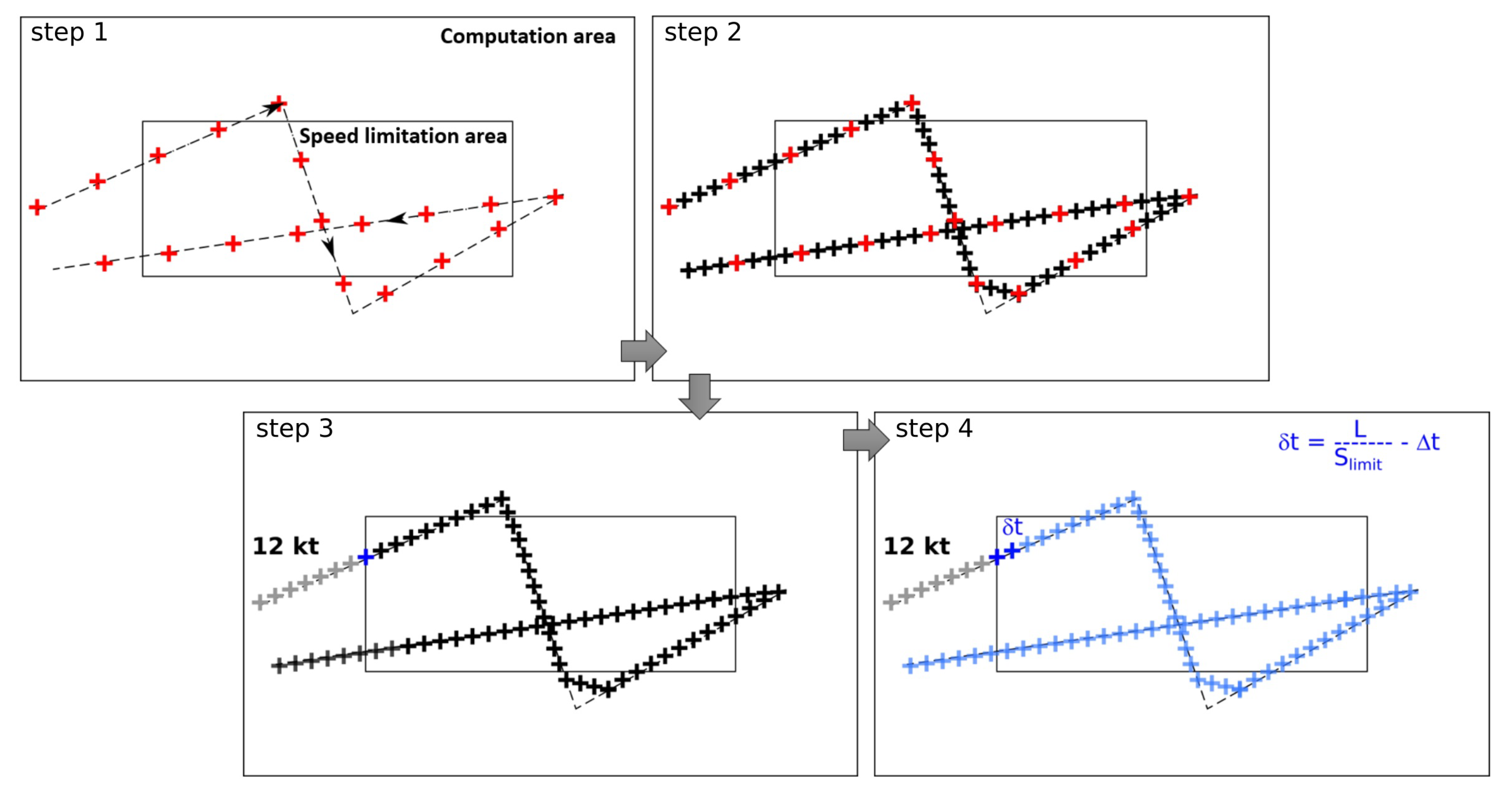
Speed limitation acts in two different ways: by reducing the source levels (according to RANDI models) and redistributing the sources in space and time. In this study, SR is simulated by modifying the AIS dataset in terms of speed and ships routes, in accordance with a speed limitation policy inside a selected SLA. The four steps that permit the creation of a modified AIS dataset are described below and illustrated in in
Figure 1.
Step 1: Retracing the route of a specific vessel through AIS data;
Step 2: Resampling of the AIS data along the route;
Step 3: Identification of the vessel entrance in the SLA;
Step 4: Estimation of the vessel speed for each section of the path inside the SLA; if the speed exceeds the speed limit, a delay is applied to subsequent AIS emissions in order to mimic the vessel speed being equal to the limitation speed.
In order to limit potential transient effects at the onset of the measure, in the simulated dataset, the measure is initiated 3 days prior to the experimentation period.
2.3. Computation of Source Levels
In order to find the source level radiated from a position, a traffic density map is computed based on the collected AIS data in the region and in the period of time considered. For a given observation period (6 h in this study), the density is considered as the time spent by a category of ships in a mesh within the observation period. In order to tackle the data gap inherent to AIS data and amplified by the existence of locally insufficient data cover, the hypothesis is made that ship trajectories between successive AIS emissions are linear, and routes are retraced by linear interpolation.
For a single ship, the SL is computed at a 5 m depth following the RANDI 3.1 model (Breeding et al., 1996, (Equation (
1)). Two parameters control this model: speed the (
s) and length (
l) of the ship. According to the model, for a given frequency (
f), the emission level in dB is
where
and
are correction coefficients, and
for frequencies below 500 Hz.
In order to limit computation time and complexity, a simplification is made, and statistical quantities are derived, gathering sources within “emitting cells”. Emitting cells are the combination of all sources within a cell (expressed through the Randi 3.1 model) balanced by the amount of time that each source ship spends within the cell along its trajectory. For each emitting cell, a Monte-Carlo scheme is applied to estimate the expectancy and standard deviation of SL from a subset of randomly sampled vessels. The expected SL of the considered grid cell is the sum of the SL for each category weighted by the traffic density. This value is used as an estimate of the mean source level at the center of the mesh.
2.4. Computation of Shipping Noise Levels
Propagation losses (PLs) are computed for each receiver. In order to improve the computation time, only sources located closer than 200 km from the receiver position are considered, removing the very small contributions from distant vessels. For frequencies higher than 300 Hz, a ray-tracing code is used. For frequencies below 300 Hz, RAM (range-dependent acoustic modeling [
16]) and RAMS (
https://oalib-acoustics.org/, accessed on 16 November 2022) are used, depending on the nature of the seabed. Details on the environmental data exploited for the computation of propagation losses are given in
Section 3.4.
RLs are then computed by subtracting the PL from the SL according to the passive SONAR equation [
17]. The received position is assumed to be at the center of the cell at several depths. The resulting maps of the received level indicate propagated shipping noise levels throughout the observation period.
RL were computed for several frequencies: 30, 50, 63, 80, 100, 125, 160, 250, 500 and 800 Hz, from which levels related to third-octave bands centered on 63 Hz and 125 Hz were extracted and presented. Computations were realized for several depths: 5, 30, 50, 90, 150, 300 and 1000 m.
2.5. Evaluating the Effect of the Measure
The effectiveness of the measure is analyzed by computing the difference (
) between the shipping noise estimated in the case in which the measure applies and the shipping noise computed for a reference state, as in Equation (
3). In the following,
represents an effect value.
where
is the received level when applying the measure, and
is the reference received level without speed reduction. An effective measure would lead to negative
values, whereas a counterproductive measure would lead to positive
values. In the computation of
, the considered noise level at a specific location is the maximum noise level obtained across the depths considered in the computation, i.e., the maximum level over the sampled water column.
2.6. Accounting for Temporal Variability in the Analysis
Ship traffic density varies over time at multiple scales (daily, monthly and yearly), and shipping noise also exhibits important temporal variability. Applying the proposed mitigation measure can significantly change the dynamics of traffic, potentially leading to high variability in the effect value (). This variability must be considered in the analysis in order to provide a complete understanding of the benefits a measure represents (regarding the environmental status).
To this end, the effect of a measure is assessed over a monthly scale by computing with an observation window of 6 h. The set of values calculated over time is noted (). Temporal assessment at a monthly scale is justified by the known dynamic of sound speed profiles, their temporal sampling and the monthly independent distribution of the modeled traffic noise levels in the frequency bands centered on 63 and 125 Hz. A choice of observation window of 6 h leads to 124 estimates of the shipping noise during the period of assessment (1 month). Short-term contrasts can be captured, such as variations of the shipping noise between day and night, reflecting as the cycle of anthropogenic activity.
Statistical quantities are computed over the month in order to characterize the distribution of , with the first quartile , the second quartile and the third quartile , such as , and , where is the cumulative distribution function (CDF) of . For the sake of clarity, the first, second and third quartiles are referred to as , and , respectively hereafter. If a measure is effective 100% of the time, then all of the samples of the distribution are expected to be negative, i.e., max() < 0. A measure acting on the shipping traffic should necessarily redistribute the sources of noise. For this reason, even in the case of an effective measure, it could be expected that a small percentage of the time, the redistribution of sources related to the measure would locally act counterproductively and provide positive values. Looking at the third quartile of the distribution permits, in particular, identification of areas exhibiting a counterproductive effect more than 25% of the time (i.e., ).
Finally, estimating (zero effectiveness) allows for apprehension of the percentage of time that the measure is effective over the month. In other words, indicates that the measure is efficient more than 50% of the time, and indicates that the measure is counterproductive more than 50% of the time. Three indicators were chosen for analysis of the temporal variability of the measure:
The first, second and third quartiles of the distribution (, and , respectively) of the effect values () estimated for a 6 h time period over the month are indicators of the central tendency and spreading of the distribution;
Estimation of the CDF of for the specific value , provides the percentage of time over the month that the measure is effective (i.e., the measure is not counterproductive);
The interquartile range can be used to quantify the spread of the distribution, i.e., the extent to which the effect of the measure is stable over the considered month.
3. Application: Context of the Experiment
3.1. Speed Limitation Area
The effect of speed limitation measures on shipping noise is assumed to vary depending on the environmental and shipping context. The largest variety of contexts possible should studied. The selected simulation zone must large enough to encompass deep and shallow water environments and include diversified shipping traffic.
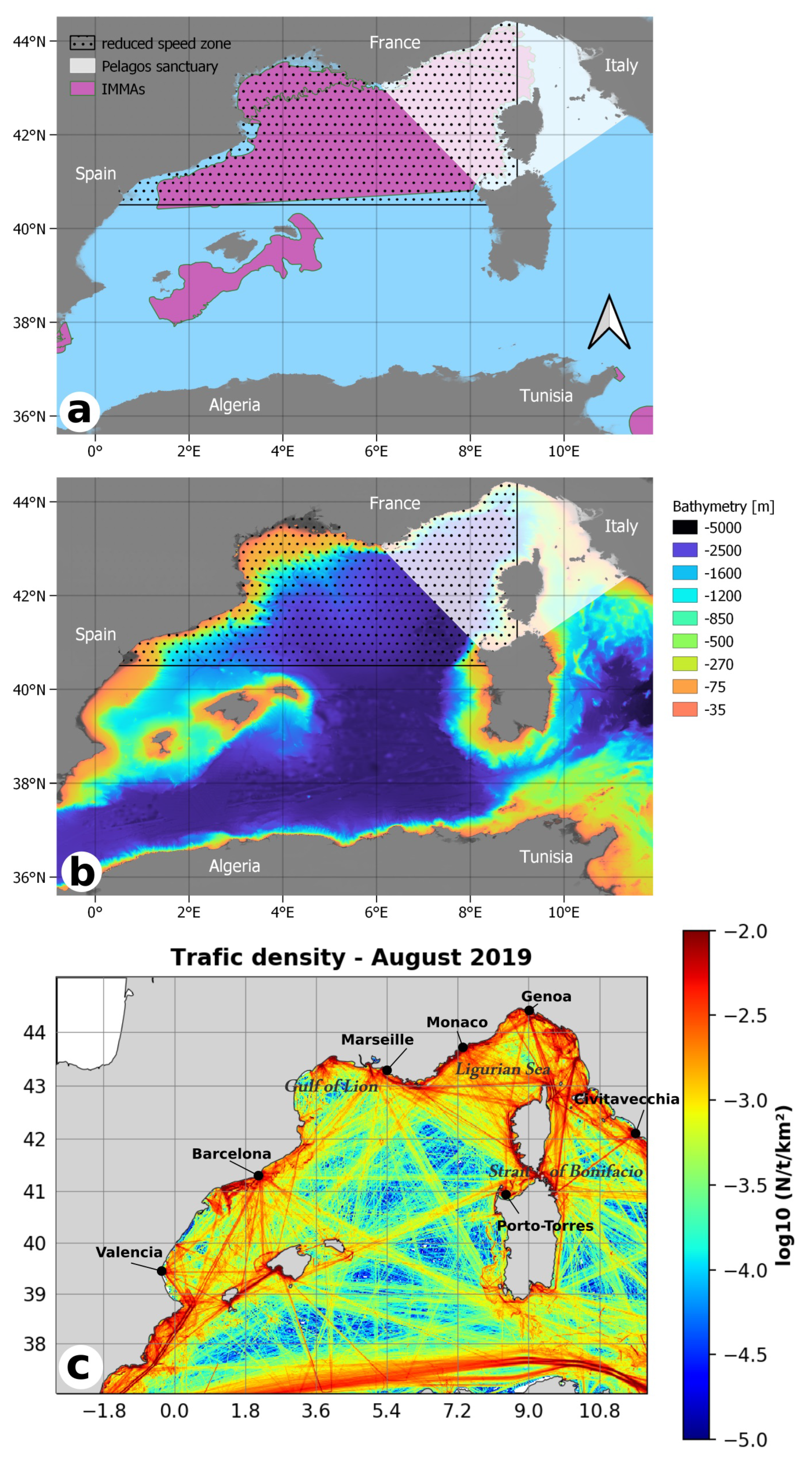
The selected zone is the Northwest Mediterranean Sea Slope and Canyon System Important Marine Mammal Area (IMMA), a zone of particular ecological interest for fin whales, sperm whales and Risso’s dolphins. It has a surface area of 145,297 km
and includes a part of the Pelagos Sanctuary, a protected area for Mediterranean marine mammals (
Figure 2). In the study area, French, Spanish, Italian and Monacan administrations, as well as stakeholders, have supported an application from the European Commission submitted to the IMO for a future particularly sensitive sea area (PSSA) in the Northwestern Mediterranean Sea in order to prevent and reduce collisions between large whales and ships and reduce anthropogenic stresses on marine mammals.
The zone includes both coastal and offshore environments. Bathymetry varies from shallow to deep waters, with maximum water depths of approximately 2800 m. The sea bottom is mostly composed of mud (vase) and, in very few locations, of sand.
In the selected zone, traffic is mostly composed of intra-European commercial activity, with a large amount of cargo, bulk, chemical and container ships and tankers. Passenger and vehicle transportation account for the second most abundant type of activity. In this zone, the traffic is characterized by a strong seasonality. During the summer, passenger vessels increase their activity, and the amount of pleasure craft increases drastically, particularly close to the shore but also offshore. In particular, small vacation vessels, which are not subject to regulation in terms of AIS emissions, may contribute locally to the underwater noise environment, in particular in coastal areas [
18,
19]. Moreover data from fishing vessels (VMS) can be difficult to obtain in some places and are sometimes absent of AIS catalogs. These non-AIS data were not accounted for in this study. Close to the reduction zones, there are some important and smaller harbors, such as Marseilles, Barcelona, Genoa, La Spezia, Livorno and Valencia. Ships in that zone are mostly routing between these harbors or between one of these harbors and either the Gibraltar or the Sicilia Strait.
3.2. Experimentation Period
The chosen period is a driving parameter. Notably, (1) non-anthropogenic noise, as well as the propagation parameters, vary throughout the year due to changes in the meteorological regime, ocean currents and seasonality; and (2) the traffic density varies from one period to another over the year. To address this last point, the month of August is chosen to realize the experiment, as it is the busiest month of the year in the chosen area, notably in relation to vacation activities [
20,
21,
22]. A full month is chosen to conduct the computation. Because it is assumed that modifying the AIS to mimic a speed limitation, a transient effect would apply at the beginning of the application period, the computation of the speed limitation simulated dataset is initiated 3 days prior to the first of August, whereas the shipping noise computation is initiated on the first of August.
3.3. Speed Limit
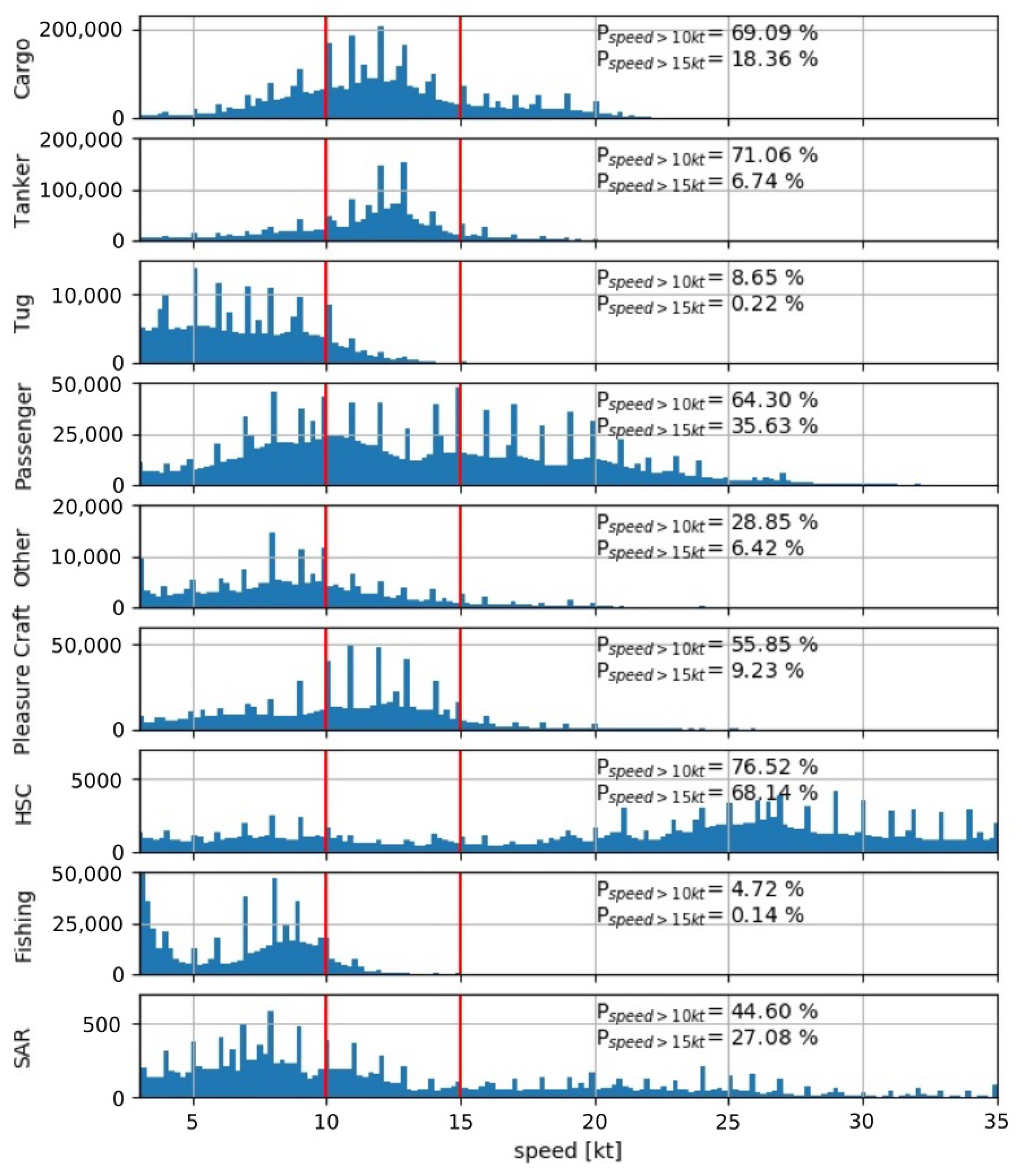
Figure 3 presents the distribution of speeds observed in AIS data for the nine categories of ships the most present in the western Mediterranean Sea during the month of August 2019. Peaks can be noted at integer values in
Figure 3 because the speed indicated in AIS data often corresponds to the speed set point, which is expressed as integer in kn, rather than the true vessel speed. As observed in the figure, except for high-speed craft (HSC), most vessels travel below 30 kt. Vessel often exceeding 15 kt include cargo ships, HSC and passenger vessels, and vessels often navigating with a speed between 10 and 15 kt include cargo tankers, passengers vessels and pleasure craft.
Based on these observations and on the ECHO program, which proposed an adjusted speed limit of between 10 and 14 kt, two speed limits were chosen for two independent experiments: 10 kt and 15 kn.
3.4. Data of the Experiment
3.4.1. AIS Data
For this work, AIS data were purchased from Exact Earth, accessed on 16 November 2022 (
www.spire.com). The set includes terrestrial and satellite AIS data that cover the Mediterranean Sea and the entire year of 2019. The fields that were used in the study are the MMSI, vessel length, vessel type and positions over time. The following vessel types were considered: cargo, tanker, HSC, tug, SAR, passenger, sailing, spare, pilot, pleasure craft, fishing, dredging, military, port tender, diving, WIG, towing, law enforcement, vessel with anti-pollution equipment, ships not party to armed conflict and medical transport, and the remaining vessels are referenced as ‘UNAVAILABLE’, ‘unknown’, ‘not available’, ‘reserved’ or ‘other’.
3.4.2. Environmental Data
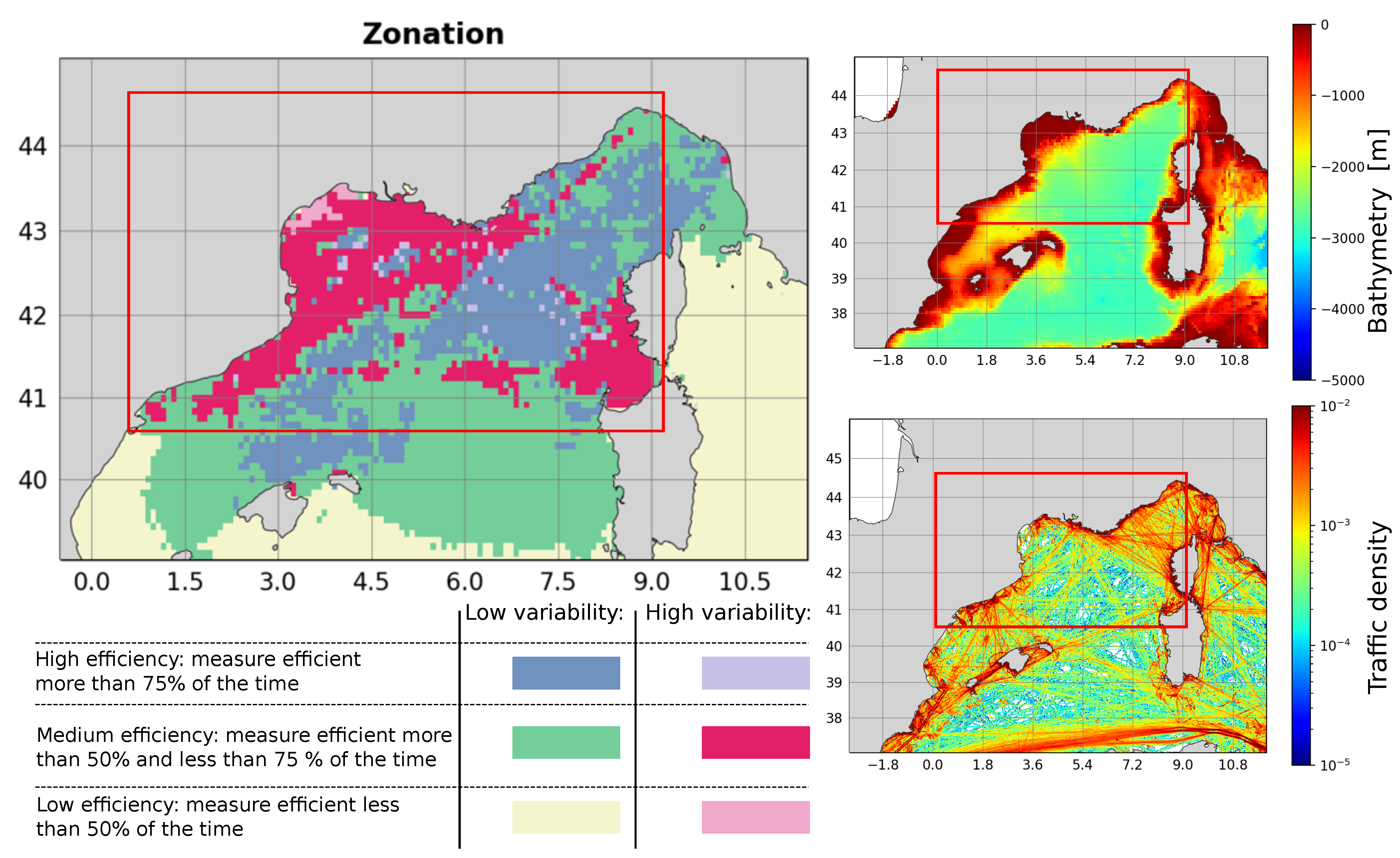
In the western Mediterranean Sea, the bathymetry is marked by important contrasts, with depths reaching 5000 m (
Figure 2a). The bathymetry data used in this work are provided by the General Bathymetric Chart of the Oceans (GEBCO) with a resolution of 5 arc minutes. The nature of the seabed is documented through data provided by the French naval hydrographic and oceanographic service (Shom,
http://data.shom.fr/, accessed on 16 November 2022) at a resolution of 15 arc minutes and is mostly composed of mud. The sound celerity dataset is composed of monthly SSP provided by Shom.
4. Results
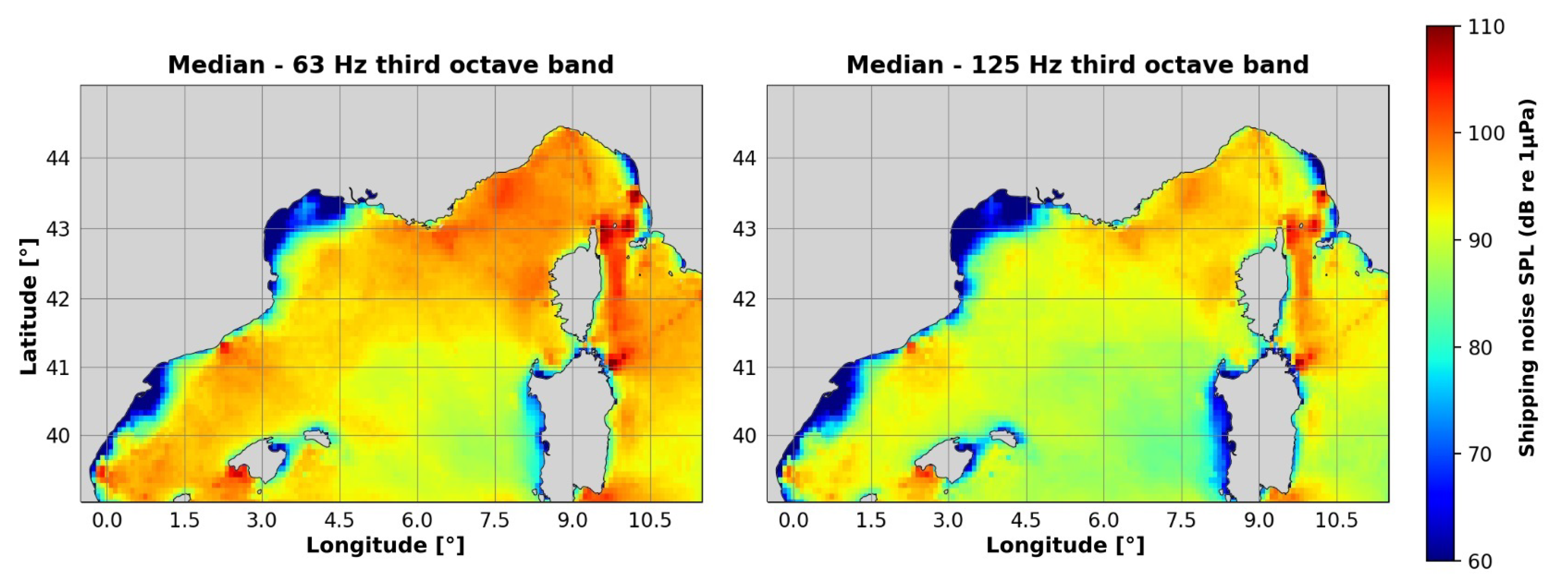
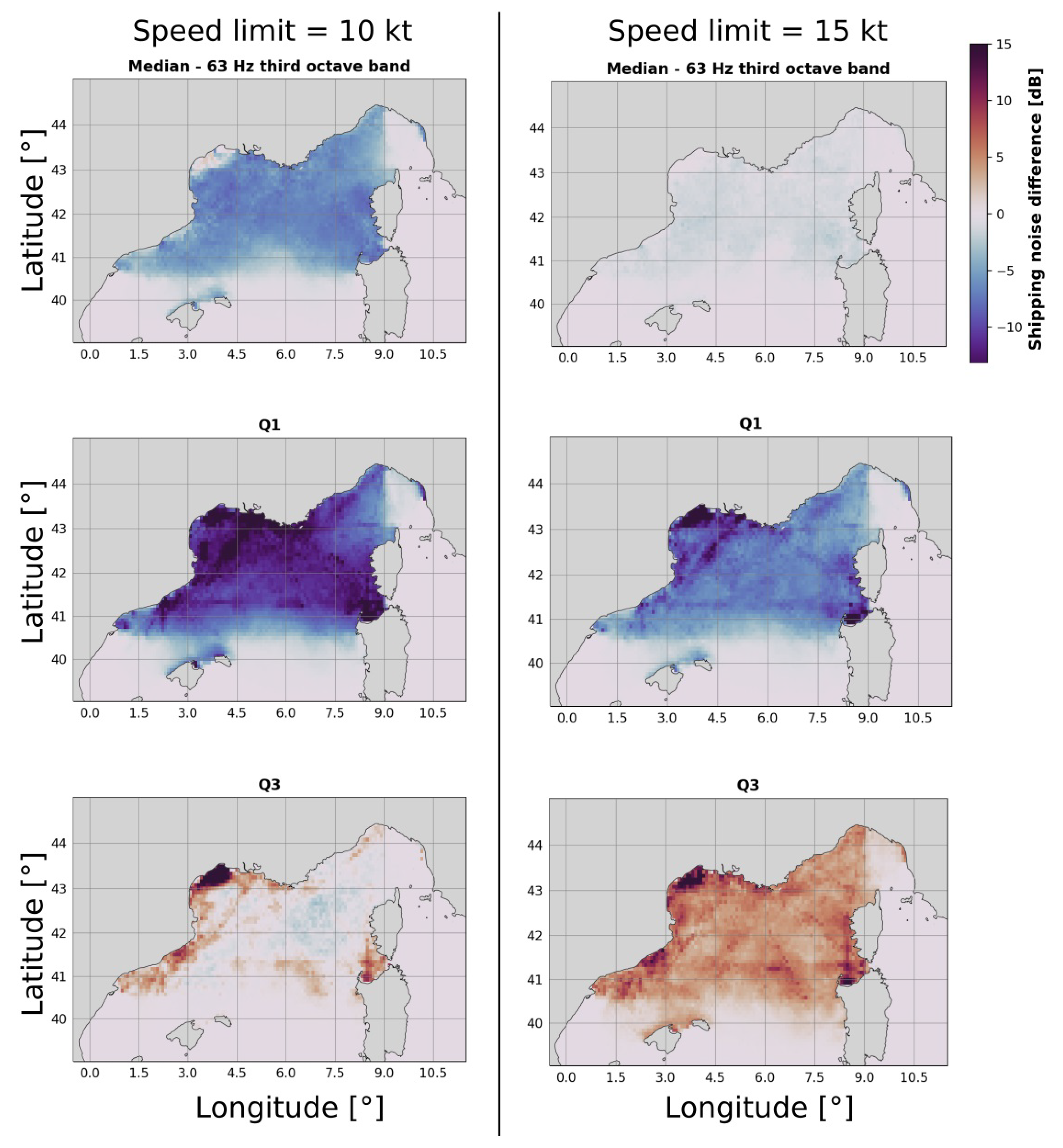
The shipping noise maps were computed in the reference case and in the two cases of speed limitation (15 and 10 kt) for each 6 h time windows. For the reference case,
Figure 4 presents the maximum of the median shipping noise within computed depths over the experimental period for the third octave frequency bands centred on 63 and 125 Hz. The median, as well as the first and third quartiles of the
distribution, is presented in the case of speed limits of 10 and 15 kt in
Figure 5. In the case of a speed limit at 10 kt, the median shows a negative central tendency for the
value (from zero to −6 dB depending on the location), indicating that the measure generally produced a decrease in shipping noise (as in the first set of experiments).
Zones with particularly low appear, as well as zones with particularly high , in agreement with the first set of experiments (some major traffic lanes, as well as crowded harbors and bottleneck areas). Where these zones overlap, the effects of the measure are very variable in time, and the effectiveness lacks stability.
The results show that in the 15 kt speed reduction case, the central tendency (median) is very close to
, suggesting a zero effectiveness, and
and
are of nearly opposite values, highlighting areas of increased variability in effectiveness (
, particularly low;
, particularly high). This very low effectiveness could be anticipated given that very few vessels exceed 15 kt (
Figure 5); therefore, the measure impacts a very limited number of vessels. Below, we focus on the case of a 10 kt speed limitation.
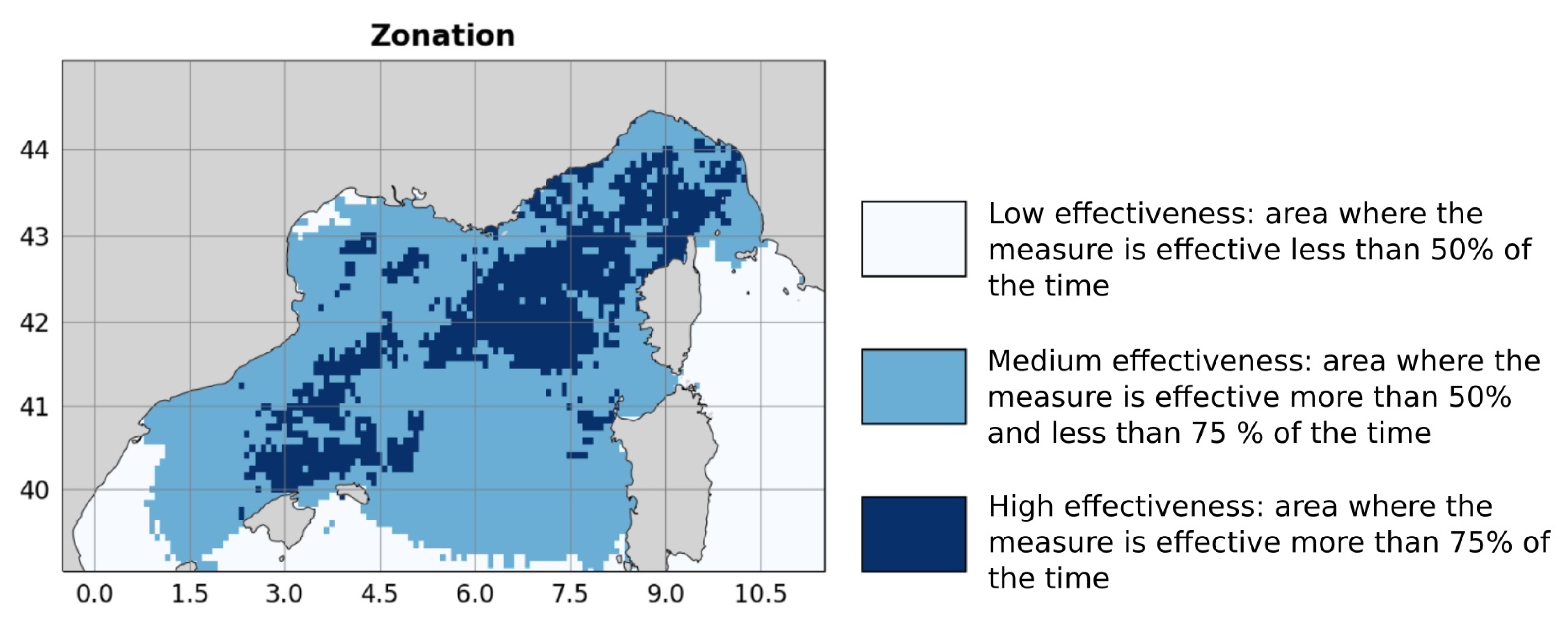
In order to capture the dynamics of the effectiveness of the measure, the second indicator consists of calculating the percentage of time that the measure is effective (
). This indicator is computed over the entire area in the case with a speed limit of 10 kt. We attributed a low effectiveness to percentages lower than 50%, a medium effectiveness to percentages between 50 and 75% and a high effectiveness to percentages higher than 75%; the results are presented in
Figure 6.
From this indicator, it is observed that:
Except for the Gulf of Lion, which is a very shallow-water area, the entire speed reduction zone experiences at least a medium effectiveness, i.e., at least 50% of the time, the speed reduction measure at 10 kt results in a decrease in shipping noise;
Some zones present a high effectiveness, mostly in deep-water areas (>2000 m). No clear relation can be derived between shipping traffic characteristics and the possibility a high-efficiency measure;
Deep-water areas (>1000 m) outside of the speed reduction zone and along its boundaries present a medium to high effectiveness. This effect is related to the propagation of sounds that can occur across large distances in deep-water environments.
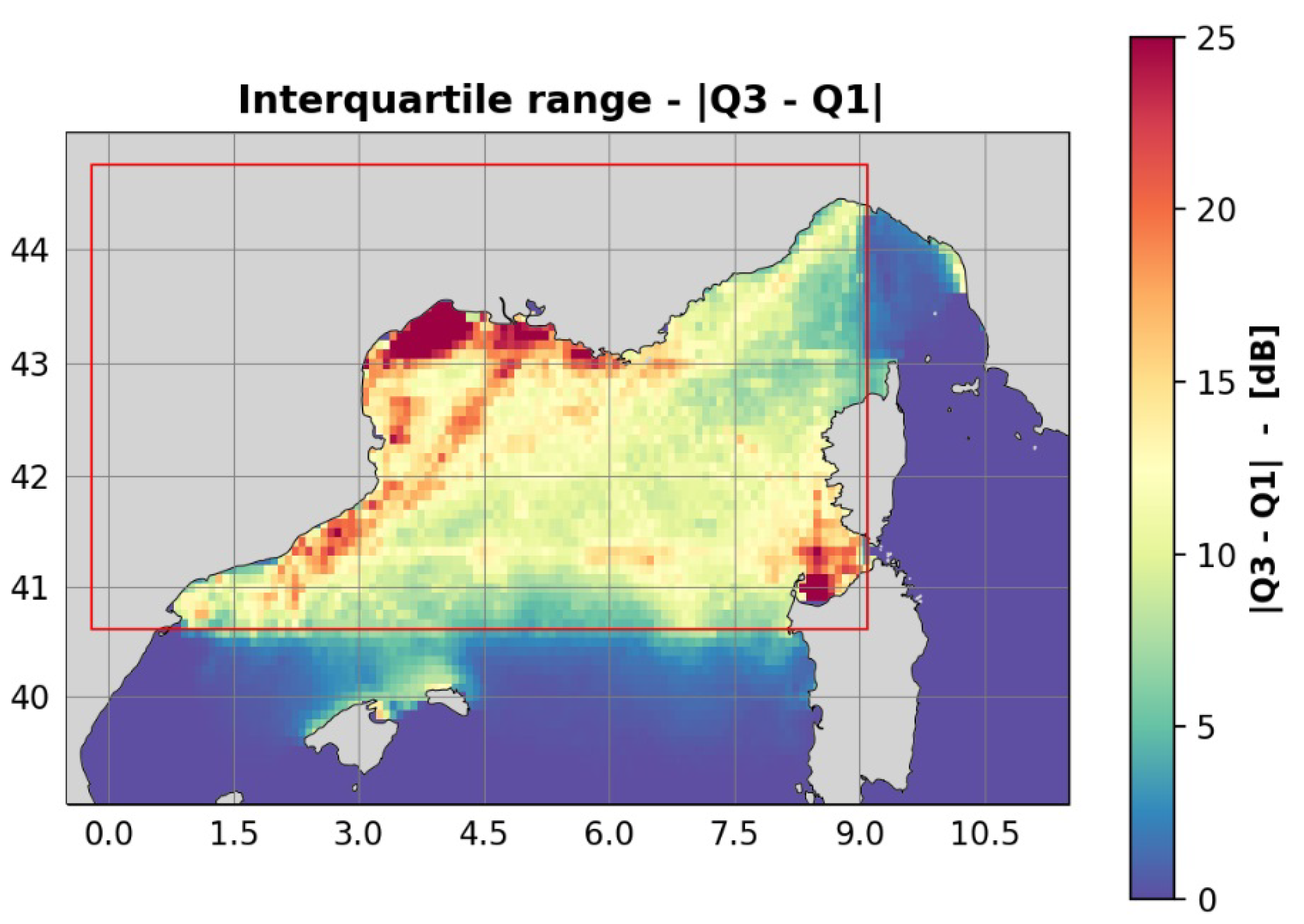
The third indicator aims to assess the stability of the effects of the measure. This is explored through the spread of the distribution of
, which is quantified by the interquartile range
in dB, as it is robust to extreme values. In
Figure 7, the interquartile range is represented for the third-octave frequency band, i.e., 63 Hz. Most of the area appears within an interquartile range of between 5 and 10 dB. A few zones are characterized by higher interquartile ranges, reaching 25 dB: major shipping routes, the Portos Torres area and the Gulf of Lion.
Figure 8 compiles the two indicators: the effectiveness of the measure and the spread of the effect over time, presenting zones of low, medium and high effectiveness in the two case scenarios: (1) stable effects of the measure, i.e., the interquartile range is below 12 dB, and (2) unstable effects of the measure, i.e., the interquartile range is above 12 dB.
From this map, it appears that stability is difficult to achieve in shallow-water environments. In deep-water environments, unstable effects can be observed in areas where the traffic is one-dimensional (along a lane) and is not homogeneously distributed. For example, a modification of the traffic along the Porto Torres–Barcelona lane will lead to an unstable modification of the shipping noise in the surrounding zone. On the contrary, in the Ligurian Sea, where many lanes cross and cover the area, the sources are evenly distributed at the sea surface, and the effect of speed reduction is quite stable.
If a medium effectiveness is observed outside of the speed limitation zone, along its boundaries, it can be noted that this effectiveness seems to be stable over time.
5. Discussion
In the next paragraphs, we tackle the methodological limits of this study.
A first limit concerns the noise model employed. It is very difficult to accurately model the source noise level of a ship. Each physical phenomenon contributing to shipping noise cannot be singularly described, and empirical models are preferred when conducting large-scale studies with multiple complex sources [
23], such as the present study. The RANDI3.1 empirical model employed in this study is accurate in a very specific context. Several characteristics that are not accounted for in the RANDI3.1 model might still impact the source levels, such as vessel weight, engine type and age and hull characteristics.
Because the engines of high-speed vessels (30 kt) might not be suited for low-speed navigation, extra noise might be produced by such vessels when navigating below the speed limitations advised by VSR programs. An analogous effect was analyzed in [
24] in the case of greenhouse gas emissions. This assumed extra noise component is very likely to occur but cannot be accounted for without an extensive study to explore whether it is negligible—and if not, how to model it.
Such measures can seem difficult to apply in large zones. For this reason, other measures are sometimes considered, such as establishing areas to be avoided [
25]. The question of the compliance of the measure was examined, and a general analysis is provided in [
26]. The cost of slowing down vessels may drastically limit such measures to small areas. In order to provide some orders of magnitude, for a navigation between Barcelona and the Strait of Bonifacio (approximately 316 nm), navigating at 30, 20, 15 and 10 kt would take approximately 10 h 30 min, 15 h 45 min, 21 h and more than 31 h 30 min, respectively. Furthermore, safety issues may be at stake. Although a slow navigation should, in theory, limit collisions, it increases the vessel density in strategic areas such as harbors, locally decreasing navigation safety.
Finally, the methodology does not account for “non-AIS” motorized vessels, which are known to be locally dominate the high-frequency underwater soundscape (125, third-octave band and higher), increasing shipping noise levels in coastal shallow water areas where they sometimes abound, as observed in [
18,
27] by investigating AIS data and acoustic recordings in coastal Danish waters and in the San Francisco Bay, respectively. Such recreational vessels often travel at high speed and might be affected by speed reduction measures such those as tested in this work, potentially increasing the positive effect of the measure.
In this article, we chose to focus on strict speed limitation. However, other ways of articulating a speed reduction measure can be considered. For example, decreasing speed by a certain percentage of normal speed could be interesting, as this limits the economic impact and important delays, perhaps making this type of measure easier to apply in a large area. Targeting only certain categories of ships or only ships exceeding certain values of lengths and speeds could help to focus the measure on very noisy vessels, limiting the economic impact of the measure. Finally, an adaptive measure that evolves throughout the year to accommodate intense and less intense traffic periods could also be envisioned.
6. Conclusions
This work presents a methodology to analyze the repercussions of a speed limitation measure on shipping noise over a large area presenting variable environmental contexts. This methodology is based on the comparison of modeled shipping noise in a reference case (true traffic and true speed) with a hypothetical case of speed limitation simulated within a selected zone. Navigation speed limitation is a mitigation measure that is known to generally reduce underwater shipping noise. This general effect is clearly identified in the results of the present study. Nevertheless, the effect is expected to vary depending on the traffic and environmental context. Despite the limitations of the methodology (drastic speed limit that may not meet economic or safety expectations, incomplete source model that tends to emphasize the role of speed in the radiated sources of noise and incomplete data), this spatialized and high-resolution (5 arc min and estimations over 6 h time slots) study contributes insights into this expected complexity, clearly showing that the environment and nature of traffic are major parameters that control the effect of the speed limitation.
Rather than measuring the shipping noise reduction in dB, the SR effect was quantified in terms of quartiles of the shipping noise difference to qualify the effectiveness and interquartile range to qualify the temporal stability of the measure. Cumulative distribution functions were used to estimate the percentage of time that the measure is effective (decrease in shipping noise).
The general observed effects of a speed limitation on shipping noise is shown to be primarily dependent on the traffic context and the environment, such as the bathymetry. These dependencies and effects are summarized in
Table 1.
As speed limitation measures seem effective in deep-water environments and present instability in shallow-water environments, complementary measures should be explored to address underwater shipping noise mitigation in shallow-water areas. For example, setting an area of avoidance for traffic could be an efficient measure in shallow-water environments, as the sources redirected along external traffic paths could possibly not be propagated across long distances due to shallow bathymetry.
In conclusion, it seems that the proposed measure could be advantageous if applied with a very restricted speed limit (15 kt has a limited effect, whereas a 10 kt speed limit may be too restrictive for the entire area), and additional marine space planning studies could be conducted to investigate the possibility of combinations of areas with different speed limits. The proposed method could also provide other benefits, such as a reduction in other forms of pollution, including CO emissions, and ship strikes. Dedicated studies are required to assess potential synergies, and metrics of combined effectiveness should be developed.
Author Contributions
Conceptualization: L.C., B.O., F.L.C. and M.L.; Methodology: L.C., B.O., F.L.C., M.L. and D.D.; Script development, data preparation and processing: M.L. and D.D.; Formal analysis and investigation: M.L., B.O. and L.C.; Writing—original draft preparation: M.L.; Writing—review and editing: L.C., B.O., F.L.C. and D.D.; Supervision: L.C., B.O. and F.L.C.; Project administration, funding acquisition and resources (data acquisition): L.C. and B.O. All authors have read and agreed to the published version of the manuscript.
Funding
This research was funded by the DG Environment of the European Commission within the call “DG ENV/MSFD 2020” Marine Strategy Framework Directive (MSFD) and the EMFF (European Maritime and Fisheries Fund) in the context of the European project QUIETSEAS (agreement 110661/2020/839603/SUB/ENV.C.2.
https://quietseas.eu/, access on 16 November 2022).
Institutional Review Board Statement
Not applicable.
Informed Consent Statement
Not applicable.
Data Availability Statement
Acknowledgments
The authors wish to thank the QUIETSEAS project partners: CTN, ACCOBAMS, POLIMI-DICA, HCMR, IzVRS, SPA/RAC, MHD, DFMR and ICES.
Conflicts of Interest
The authors declare no conflict of interest. The funders had no role in the design of the study; in the collection, analyses or interpretation of data; in the writing of the manuscript; or in the decision to publish the results.
Abbreviations
The following abbreviations are used in this manuscript:
| AIS | Automatic identification system |
| VMS | Vessel monitoring system |
| SL | Source level |
| SPL | Sound pressure level |
| RL | Received levels |
| PL | Propagation loss |
| SLA | Speed limitation area |
| SR | Speed reduction |
| VSR | Voluntary speed reduction |
| MSFD | Marine strategy framework directive |
| CDF | Cumulative density function |
| IMMA | Important marine mammal area |
References
- Tournadre, J. Anthropogenic pressure on the open ocean: The growth of ship traffic revealed by altimeter data analysis. Geophys. Res. Lett. 2014, 41, 7924–7932. [Google Scholar] [CrossRef]
- Weilgart, L. The Impact of Ocean Noise Pollution on Fish and Invertebrates; Report for OceanCare; OceanCare: Wädenswil, Switzerland, 2018. [Google Scholar]
- Edmonds, N.J.; Firmin, C.J.; Goldsmith, D.; Faulkner, R.C.; Wood, D.T. A review of crustacean sensitivity to high amplitude underwater noise: Data needs for effective risk assessment in relation to UK commercial species. Mar. Pollut. Bull. 2016, 108, 5–11. [Google Scholar] [CrossRef] [PubMed]
- Tidau, S.; Briffa, M. Review on behavioral impacts of aquatic noise on crustaceans. Proc. Mtgs. Acoust. 2016, 27, 010028. [Google Scholar] [CrossRef]
- Roberts, L.; Pérez-Domínguez, R.; Elliott, M. Use of baited remote underwater video (BRUV) and motion analysis for studying the impacts of underwater noise upon free ranging fish and implications for marine energy management. Mar. Pollut. Bull. 2016, 112, 75–85. [Google Scholar] [CrossRef] [PubMed]
- Vazzana, M.; Ceraulo, M.; Mauro, M.; Papale, E.; Dioguardi, M.; Mazzola, S.; Arizza, V.; Chiaramonte, M.; Buscaino, G. Effects of acoustic stimulation on biochemical parameters in the digestive gland of Mediterranean mussel Mytilus Gall. (Lamarck, 1819). J. Acoust. Soc. Am. 2020, 147, 2414–2422. [Google Scholar] [CrossRef]
- Chion, C.; Turgeon, S.; Cantin, G.; Michaud, R.; Ménard, N.; Lesage, V.; Parrott, V.; Beaufils, P.; Clermont, Y.; Gravel, C. A voluntary conservation agreement reduces the risks of lethal collisions between ships and whales in the St. Lawrence Estuary (Québec, Canada): From co-construction to monitoring compliance and assessing effectiveness. PLoS ONE 2018, 13, e0202560. [Google Scholar] [CrossRef]
- Pine, M.K.; Hannay, D.E.; Insley, S.J.; Halliday, W.D.; Juanes, F. Assessing vessel slowdown for reducing auditory masking for marine mammals and fish of the western Canadian Arctic. Mar. Pollut. Bull. 2018, 135, 290–302. [Google Scholar] [CrossRef]
- Joy, R.; Tollit, D.; Wood, J.; MacGillivray, A.; Li, Z.; Trounce, K.; Robinson, O. Potential Benefits of Vessel Slowdowns on Endangered Southern Resident Killer Whales. Front. Mar. Sci. 2019, 6, 344. [Google Scholar] [CrossRef]
- ZoBell, V.M.; Frasier, K.E.; Morten, J.A.; Hastings, S.P.; Peavey Reeves, L.E.; Wiggins, S.M.; Hildebrand, J.A. Underwater noise mitigation in the Santa Barbara Channel through incentive-based vessel speed reduction. Sci. Rep. 2021, 11, 18391. [Google Scholar] [CrossRef]
- Jensen, C.M.; Hines, E.; Holzman, B.A.; Moore, T.J.; Jahncke, J.; Redfern, J.V. Spatial and Temporal Variability in Shipping Traffic Off San Francisco, California. Coast. Manag. 2015, 43, 575–588. [Google Scholar] [CrossRef]
- Moore, T.J.; Redfern, J.V.; Carver, M.; Hastings, S.; Adams, J.D.; Silber, G.K. Exploring ship traffic variability off California. Ocean Coast. Manag. 2018, 163, 515–527. [Google Scholar] [CrossRef]
- Redfern, J.V.; Becker, E.A.; Moore, T.J. Effects of Variability in Ship Traffic and Whale Distributions on the Risk of Ships Striking Whales. Front. Mar. Sci. 2020, 6, 793. [Google Scholar] [CrossRef]
- Ollivier, B.; Le Courtois, F.; Bazile Kinda, G.; Ratsivalaka, C.; Sarzeaud, O.; Boutonnier, J.M. Analysis of the comprehensiveness of AIS data sets: Application to the underwater noise modelling at basin scale. In Proceedings of the OCEANS 2019—Marseille, Marseille, France, 17–20 June 2019; pp. 1–6. [Google Scholar] [CrossRef]
- Le Courtois, F.L.; Kinda, G.B.; Boutonnier, J.M.; Stéphan, Y.; Sarzeaud, O. Statistical ambient noise maps from traffic at world and basin scales. In Acoustic and Environmental Variability, Fluctuations and Coherence; Institute Of Acoustics: Cambridge, UK, 2016. [Google Scholar]
- Collins, M.D.; Westwood, E.K. A higher-order energy-conserving parabolic equqation for range-dependent ocean depth, sound speed, and density. J. Acoust. Soc. Am. 1991, 89, 1068–1075. [Google Scholar] [CrossRef]
- ISO. ISO 18405: 2017. Underwater Acoustics—Terminology. Available online: https://cdn.standards.iteh.ai/samples/62406/d4e330b42f944401bf8522761712519b/ISO-18405-2017.pdf (accessed on 16 November 2022).
- Hermannsen, L.; Mikkelsen, L.; Tougaard, J.; Beedholm, K.; Johnson, M.; Madsen, P.T. Recreational vessels without Automatic Identification System (AIS) dominate anthropogenic noise contributions to a shallow water soundscape. Sci. Rep. 2019, 9, 15477. [Google Scholar] [CrossRef]
- Magnier, C.; Gervaise, C. Acoustic and photographic monitoring of coastal maritime traffic: Influence on the soundscape. J. Acoust. Soc. Am. 2020, 147, 3749–3757. [Google Scholar] [CrossRef]
- Campana, I.; Angeletti, D.; Crosti, R.; Luperini, C.; Ruvolo, A.; Alessandrini, A.; Arcangeli, A. Seasonal characterisation of maritime traffic and the relationship with cetacean presence in the Western Mediterranean Sea. Mar. Pollut. Bull. 2017, 115, 282–291. [Google Scholar] [CrossRef]
- Esteve-Perez, J.; Garcia-Sanchez, A. Determination of Seasonality Patterns in the Transport of Cruise Travellers Through Clustering Techniques. J. Navig. 2019, 72, 1417–1434. [Google Scholar] [CrossRef]
- Esteve-Perez, J.; Garcia-Sanchez, A.; Muñoz-Paupie, A. Cruise Traffic Seasonality Patterns in the Western Mediterranean and the Adriatic Sea: A Challenge to Port Operators. Coast. Manag. 2019, 47, 362–386. [Google Scholar] [CrossRef]
- Yan, X.; Song, H.; Peng, Z.; Kong, H.; Cheng, Y.; Han, L. Review of research results concerning the modelling of shipping noise. Pol. Marit. Res. 2021, 2, 102–115. [Google Scholar] [CrossRef]
- Psaraftis, H. Speed Optimization vs. Speed Reduction: The Choice between Speed Limits and a Bunker Levy. Sustainability 2019, 11, 2249. [Google Scholar] [CrossRef]
- Vanderlaan, A.S.M.; Taggart, C.T. Efficacy of a Voluntary Area to Be Avoided to Reduce Risk of Lethal Vessel Strikes to Endangered Whales. Conserv. Biol. 2009, 23, 1467–1474. [Google Scholar] [CrossRef] [PubMed]
- Morten, J.; Freedman, R.; Adams, J.D.; Wilson, J.; Rubinstein, A.; Hastings, S. Evaluating Adherence With Voluntary Slow Speed Initiatives to Protect Endangered Whales. Front. Mar. Sci. 2022, 9. [Google Scholar] [CrossRef]
- Cope, S.; Hines, E.; Bland, R.; Davis, J.D.; Tougher, B.; Zetterlind, V. Multi-sensor integration for an assessment of underwater radiated noise from common vessels in San Francisco Bay. J. Acoust. Soc. Am. 2021, 149, 2451–2464. [Google Scholar] [CrossRef] [PubMed]
| Disclaimer/Publisher’s Note: The statements, opinions and data contained in all publications are solely those of the individual author(s) and contributor(s) and not of MDPI and/or the editor(s). MDPI and/or the editor(s) disclaim responsibility for any injury to people or property resulting from any ideas, methods, instructions or products referred to in the content. |
© 2023 by the authors. Licensee MDPI, Basel, Switzerland. This article is an open access article distributed under the terms and conditions of the Creative Commons Attribution (CC BY) license (https://creativecommons.org/licenses/by/4.0/).


