Prediction of Shipping Noise in Range-Dependent Environments

Abstract

A prediction model for shipping noise in range-dependent environments based on coupled-mode theory is presented, as an enhancement to existing adiabatic normal-mode approaches without a significant increase in computational effort. Emphasis is placed on the categorization of environmental changes and precalculation and storage of eigenvalues, eigenfunctions and coupling matrices, such that they can be looked up and restored to efficiently compute the acoustic field of arbitrary noise source distributions over a given sea area. Taking into account that the water depth is the primary factor determining the number of propagating modes for a particular frequency, coupling is applied only in the case of changing bathymetry, whereas changes in the water sound-speed profile and/or the geoacoustic characteristics are treated adiabatically. Examples of noise calculations are given for benchmark setups in the Eastern Mediterranean Sea and comparisons with fully adiabatic predictions are drawn. Moreover, the effect of applying range propagation limitations in a numerical propagation model for shipping noise predictions is demonstrated.

1. Introduction

The concern about the impact of anthropogenic noise on marine life has led to intensification of efforts to map and study the underwater noise field. Aiming at the establishment of good environmental status in the sea areas surrounding Europe, the EU Marine Strategy Framework Directive (MSFD) [1] addresses—among others—underwater noise pollution under Descriptor 11 [2,3]. Similarly, the US National Oceanic and Atmospheric Administration (NOAA) has developed an ocean noise strategy [4] and has established working groups to study underwater soundscapes, while Australia included characterization of anthropogenic underwater noise to better understand and manage impacts to marine life in their National Environmental Science Programme [5].

Shipping noise is a dominant component of ambient noise in the sea at lower frequencies, between 20 and 200 Hz [6]. Large ships are sources of low-frequency acoustic waves, with cavitation being the primary noise-generation mechanism together with machinery and plate vibrations [7]. Smaller ships, such as fishing vessels and pleasure craft, also produce noise, albeit usually at higher frequencies [8,9]. The present work focuses on low-frequency noise generated from large travelling ships, which propagates efficiently through the water mass and, thus, affects underwater noise levels at large distances from the major shipping lanes.

The acoustic status of an area is assessed using modelling and measurements [10]. Models are validated with field measurements and measurements can be supported with modelling. Under the prism of the EU MSFD, the combined use of measurements and models (and possibly sound maps) is the best way for member states to ascertain levels and trends of ambient noise in the relevant frequency bands [11]. Although in situ noise measurements provide valuable ground-truth data, they cannot be used for noise mapping over large sea areas. Long-term measurements do allow for the estimation of ambient noise levels and trends at the location of the measurements. Nevertheless, it is difficult to extrapolate the results to other locations, especially in areas of complicated coastline and bathymetry. Acoustic propagation modelling, in combination with advancements related to the availability of ship tracking data, can be supportive in this respect by offering a means to interpret the spatial variability of the noise field measured at different locations. However, there are a number of challenges for the acoustic modelling of shipping noise as well, concerning ship data (ship locations and acoustic signatures) and environmental data (bathymetry, oceanography, bottom type). Furthermore, another significant challenge concerns the propagation modelling and the computational burden associated with the calculation of the acoustic field produced by a large number of noise sources over a large sea area. As mentioned in a recent review paper regarding underwater noise research in support of the EU MSFD [12], regional monitoring has relied on the modelling of shipping noise based on navigation data [13,14,15,16,17,18,19,20], but only few published shipping noise maps of European waters have been validated with field measurements (e.g., [18,20]), while ongoing field monitoring work within joint monitoring programs is expected to yield further validated maps at regional scale.

In recent times, ship traffic data have become readily available through the Automatic Identification System (AIS), introduced primarily as a collision avoidance aid. Large commercial ships with gross tonnage of 300 or more and passenger ships regardless of size, i.e., all ships contributing to low-frequency noise, are required to carry VHF equipment broadcasting their static and dynamic data (static meaning ship name, type, navigation status, etc., and dynamic meaning position fix, speed, direction, etc.), and receiving such data from nearby ships, within a few tens of km. AIS signals are also received by land- and satellite-based receivers, which enable worldwide ship tracking [21]. Regarding smaller crafts, commercial fishing vessels are equipped with vessel monitoring systems (VMS) which allow environmental and regulatory organizations to track and monitor fishing activities [22]. Still, there is a large number of smaller vessels not obliged to carry AIS or VMS systems, which may contribute significantly to underwater noise levels in some localized areas [23]. Furthermore, there are gaps associated with the poor coverage of certain sea areas far away from the coast; in such cases, the ship locations can be estimated through methods exploiting traffic pattern knowledge, dead reckoning and data fusion [24,25].

Regarding the noise emission levels, it is well understood that different ships have different acoustic emission characteristics. Even the same ship may have different acoustic characteristics depending on its load, navigation status, speed, maintenance condition, etc. While the noise emission levels of individual ships are unknown, data on typical acoustic signatures for different ship types can be found in the literature. Recent studies are based on the combination of measurements and AIS data of large numbers of travelling ships, taking into account propagation characteristics of the measurement sites [6,26,27,28,29,30]. Some of these analyses, e.g., [27], resulted in underestimated source levels because of the hydrophone lying in the shadow zone of the formed Lloyd’s mirror propagation pattern [31]. The ANSI/ASA S12.64-2009 standard [32] overcomes this effect by averaging over three hydrophones at different depths and short range, and source level estimates from setups close to this standard [28,31] should be treated with greater confidence. Recent systematic studies [29,30] have produced methodologies based on regression analysis for the estimation of spectral source levels at different frequencies from ship type, length and travelling speed. By combining these methodologies with real-time AIS data, the locations and strengths of individual noise sources to drive propagation models can be obtained [13]. Alternatively, statistical descriptions of shipping lanes in terms of shipping densities [33] can be used to estimate the corresponding noise source distributions [34,35].

Environmental data for the water column, in particular temperature and salinity distributions determining the sound-speed distribution and affecting the propagation conditions, can be obtained from direct measurements as well as from operational ocean circulation models and associated databases such as the World Ocean Atlas [36] and Copernicus [37]. Bathymetry can be retrieved from databases such as the ETOPO global relief model [38] or the 2020 version of the EMODnet Digital Terrain Model for European Seas [39]. The greatest environmental unknown is related to the bottom composition, since data from direct sampling are sparse and mostly treated as confidential.

Coming to the acoustic propagation modelling, several models have been used for simulating shipping noise (see, e.g., [40]). A wave-theoretic approach, such as parabolic approximation or normal modes [41], seems to be more appropriate for low-frequency predictions. Nevertheless, considering the general problem of an ocean waveguide with complex bathymetry including both shallow and deep waters, the large number of noise sources and the large size of the computational domain (sea area of interest), one needs to seek ways to reduce the extensive computational burden. One possible solution is by exploiting similarities between different areas, such as the same water depth or sound-speed profile. An asset of the parabolic approximation is that it can handle an arbitrary variation in depth and range of the acoustic parameters of the environment (water depth, sound velocity, attenuation, etc.), essentially without additional computational cost. On the other hand, this method cannot exploit similarities between different areas. In that matter, the parabolic approximation is suitable for the calculation of the acoustic field of a specific source along a specific range-dependent transect [6,26,30], but in the case of the calculation of the acoustic field of a large number of sources over a large area, the computational burden becomes an issue.

In this case, normal-mode theory, and in particular adiabatic and coupled-mode approaches, can prove more efficient since they are based on local solutions along each propagation path [42,43,44]. Classifying the local environments in a broader sea area, based on water depth, sound-speed profile and bottom type, the corresponding vertical eigenvalue problems can be solved in advance, resulting in wavenumbers and modes at particular depths, as well as in coupling matrices between adjacent local environments. The precomputed results can be stored in a database and recovered accordingly, in order to rapidly calculate the acoustic field along each acoustic path from a particular noise source. The first attempts to predict shipping noise over large sea areas, at basin or global scales, were based on adiabatic propagation modelling [16,43] neglecting energy exchange between propagating modes. Though computationally efficient, this approach is not well-suited for areas of abrupt environmental changes giving rise to mode coupling (energy exchange between modes). Taking into account that the primary factor determining the number of propagating modes for a particular frequency is water depth, a mixed approach is proposed, in which coupling is applied in the case of variable bathymetry, whereas changes in the water sound-speed profile and/or the geoacoustic characteristics are treated adiabatically. Even so, the need to calculate and store the coupling matrices for all possible combinations of bathymetry variations has an impact on computational effort and complexity. This can be mitigated by calculating coupling matrices only between subsequent discrete water depths, as explained in the following section. The final goal is to replace the shipping noise-prediction model based on the adiabatic approach with a more complete coupled-mode-based model without considerable increase in the computational cost. This would allow for implementing the latter in operational shipping noise prediction.

The contents of this work are organized as follows: Section 2 presents the coupled-mode formulation and describes an implementation scheme for the evaluation of the noise field of a large number of noise sources (ships) over a large sea area, based on precalculated modal results for a set of local environments spanning the variability in the area of interest. In Section 3, numerical examples are used to elucidate the influence of propagation conditions, frequencies of interest and range limitations on the noise levels, as well as on the differences between adiabatic and coupled-mode calculations. Finally, Section 4 presents the main conclusions along with a discussion of the obtained results.

2. Materials and Methods

2.1. Coupled-Mode Propagation Modelling

In this section, the coupled-mode solution to the axisymmetric range-dependent propagation problem is described. Adopting a cylindrical coordinate system $(r,z)$, the source is assumed to be harmonic of circular frequency $\omega$ with time dependence $\exp (i\omega t)$ and lie on the vertical axis $(r_S=0)$ at depth $z_S$. Following Evans [45], the environment is assumed piecewise constant in range, i.e., within each range segment, extending to range $r_{\ell },\ell =1,2,\dots ,L$, the water depth $h_{\ell }$, the sound-speed profile $c_{\ell }(z)$ and the bottom characteristics—sediment thickness/type and half-space properties—are considered constant (see Figure 1).

The acoustic pressure, i.e., the solution of the Helmholtz equation, within the $\ell$th range segment can be written in the form [34].

$$P_{\ell }(r,z)={\displaystyle \sum _{m=1}^{M_{\ell }}\left[a_{m;\ell }{e}^{-i{k}_{m;\ell }(r-r_{\ell -1})}+b_{m;\ell }{e}^{i{k}_{m;\ell }(r-r_{\ell -1})}\right]}\hspace{0.17em}\sqrt{\frac{r_{\ell -1}}{r}}\hspace{0.17em}{\varphi }_{m;\ell }(z),$$

(1)

where $k_{m;\ell }$ and ${\phi }_{m;\ell }(z)$, $m=1,2,\dots ,M_{\ell }$, are the real eigenvalues and the corresponding eigenfunctions (propagating modes) of the vertical eigenvalue problem within the $\ell$th segment; it is noted that, in general, a different number of modes $M_{\ell }$ is supported in each range segment ($\ell$). The first and second term within the brackets in Equation (1) represent the forward and backward propagation, respectively, and the factors $a_{m;\ell }$ and $b_{m;\ell }$ describe the excitation of the corresponding waves. The vertical eigenvalue problem within the $\ell$th segment has the form

$$\frac{d^2{\varphi }_{m;\ell }(z)}{d{z}^2}+\frac{{\omega }^2}{c_{\ell }^2(z)}{\varphi }_{m;\ell }(z)=k_{m;\ell }^2{\varphi }_{m;\ell }(z),$$

(2)

supplemented by the conditions that ${\phi }_{m;\ell }(0)=0$ at the surface ($z=0$), ${\phi }_{m;\ell }$ and ${\rho }^{-1}d{\phi }_{m;\ell }/dz$ are continuous at the water–sediment and sediment–bottom interfaces, and finally ${\phi }_{m;\ell }$ and $d{\phi }_{m;\ell }/dz$ are vanishing as $z\to \infty$. The propagating modes, being solutions of the above eigenvalue problem, form an orthonormal set, i.e.,

$${\displaystyle \underset{0}{\overset{\infty }{\int }}\frac{1}{\rho (z)}}{\varphi }_{m;\ell }(z){\varphi }_{n;\ell }(z)dz={\delta }_{mn}\equiv \left\{\begin{array}{l}0 \mathrm{for} m\ne n\\ 1 \mathrm{for} m=n\end{array}\right.$$

(3)

The continuity of pressure at the interface between the segments $\ell$ and $\ell +1$, at the range $r_{\ell }$, can be expressed as

$$P_{\ell }(r_{\ell },z)=P_{\ell +1}(r_{\ell },z), \ell =1,\dots ,L-1$$

(4)

Substituting Equation (1) into Equation (4), and neglecting the backscattering terms, i.e., setting $b_{m;\ell }=b_{m;\ell +1}=0$, the pressure-continuity condition becomes

$${\displaystyle \sum _{m=1}^{M_{\ell }}{a}_{m;\ell }{e}^{i{k}_{m;\ell }(r_{\ell }-r_{\ell -1})}}\sqrt{\frac{r_{\ell -1}}{r_{\ell }}}{\varphi }_{m;\ell }(z)={\displaystyle \sum _{m=1}^{M_{\ell +1}}{a}_{m;\ell +1}}{\varphi }_{m;\ell +1}(z)$$

(5)

Taking the inner product of both sides with ${\phi }_{n;\ell +1}$ and exploiting the orthonormality property (Equation (3)), the excitation factors $a_{n;\ell +1}$ in the ($\ell +1$)th segment can be expressed recursively, in terms of the excitation factors $a_{m;\ell }$ in the $\ell$th segment, as follows

$$a_{n;\ell +1}={\displaystyle \sum _{m=1}^{M_{\ell }}{a}_{m;\ell }{e}^{i{k}_{m;\ell }(r_{\ell }-r_{\ell -1})}}\sqrt{\frac{r_{\ell -1}}{r_{\ell }}}\hspace{0.33em}{C}_{mn;\ell },$$

(6)

where

$$C_{mn;\ell }={\displaystyle \underset{0}{\overset{\infty }{\int }}\frac{1}{{\rho }_{\ell +1}(z)}{\varphi }_{m;\ell }}(z)\hspace{0.17em}{\varphi }_{n;\ell +1}(z)\hspace{0.17em}dz$$

(7)

is the coupling coefficient between the $m$th and $n$th mode in the segments $\ell$ and $\ell +1$, respectively. For the case $\ell =1$, the convention $r_{\ell -1}=r_1$ is made, i.e., $r_1$ is taken as reference range for both the first and the second range segments. The excitation factor in the first range segment is taken from the source condition [41] as

$$a_{m,1}=\frac{{\varphi }_{m,1}(z_S)}{{\rho }_1(z_S)\sqrt{8\pi r_1{k}_{m,1}}}{e}^{i(k_{m,1}{r}_1+\pi /4)}, m=1,\dots ,M_1$$

(8)

The adiabatic approximation can be represented by the same expressions with the only difference that the coupling matrix (Equation (7)) is replaced by a matrix of the same dimensions with ones on the main diagonal and zeros elsewhere, i.e., $C_{mn;\ell }^{(ad)}={\delta }_{mn}$.

2.2. Coupled-Mode Implementation for Shipping Noise Calculations

The prediction of shipping noise over large sea areas of complicated bathymetry, such as the Eastern Mediterranean Sea, poses big challenges associated with the calculation of the acoustic field of a large number of sources (thousands of ships) that move over time. The typical way to calculate the acoustic field of a sound source along a range-dependent section at a certain azimuth is (a) to discretize the section into a number of range segments of constant characteristics in range, (b) to solve the vertical problem in each segment, (c) to calculate the coupling matrices at the interfaces between subsequent segments, and finally (d) to evaluate the field as described in the previous subsection. This procedure must be repeated for all azimuthal directions about a source and for all sources in the area of interest, and, thus, it would be quite impractical in the case of a large sea area and a large number of sources with arbitrary distribution.

One possible solution would be to calculate the acoustic field for all possible source (ship) locations, store the results and use the ones corresponding to the actual ship distribution [46]. Though straightforward, this approach is impractical for large sea areas; e.g., for the case of the Eastern Mediterranean Basin, a resolution of 1 arc minute (~1.8 km) would result in more than one million grid points, around which the acoustic calculations should be performed and repeated for each month or season of interest.

In this work, an alternative approach is proposed. It involves the discretization of the bathymetry with a certain resolution, the categorization of the environmental variability for each month or season of interest, and the precalculation and storage of eigenvalues, eigenfunctions and coupling matrices corresponding to the resulting family of vertical problems. To reduce the computational complexity, the coupling matrices are calculated only between environments with consecutive discrete water depths. This is handled by introducing additional grid points in areas of abrupt bathymetry changes, such that the difference between water depths of adjacent range segments equals the selected bathymetry discretization step.

The above-described method can be formally postulated as follows:

A.

Precalculations

• Use a bathymetry grid for the area of interest and discretize the bathymetry with a certain resolution, e.g., 10 m;
• Define sub-areas of similar bottom characteristics (sediment type, thickness, sub bottom, etc.); this will result in a finite number of representative bottom types;
• For each month or season of interest, define sub-areas of similar sound velocity profile (SVP), e.g., through cluster analysis of available SVPs, either from measurements or from oceanographic models; this will result in a finite number of representative SVPs;
• For each combination of representative bottom type and representative SVP, solve the vertical problem, calculate and store eigenvalues and eigenfunctions (modes) for each discrete water depth, and also calculate and store the coupling matrices between subsequent depths.

B.

Acoustic field calculation

• For a particular ship distribution, group nearby ships on the calculation grid and accumulate spectral source levels;
• Loop over noise sources;
  • Loop over transects in the azimuthal;
    • Define the environment along the transect by merging grid points of equal water depth, SVP and bottom characteristics;
    • In case of abrupt depth changes, introduce additional grid points and linearly interpolate depths such that the differences between depths of adjacent range segments equals the depth resolution;
    • Selectively recall stored results (eigenvalues, eigenfunctions and coupling matrices) to calculate the acoustic field along the particular transect. Use coupling only in case of depth change; otherwise, propagate adiabatically;
  • Repeat for all transects and interpolate in the azimuthal;
• Repeat for all noise sources and accumulate the acoustic intensity at each grid point.

Thus, for each environment characterized by a certain sound-velocity profile and geoacoustic characteristics, the vertical problem is solved (the eigenvalues and eigenfunctions are calculated) for a number of discrete depths, and the coupling matrices are evaluated only between subsequent discrete depths. The fact that the coupling matrices are not calculated for all possible combinations of discrete depths saves a lot of storage space and also enables efficient recovery for acoustic field calculation. Furthermore, in the case of very steep bathymetry, intermediate grid points are added such that the interpolated depths comply with the discretization step (see Figure 2).

Mode coupling is applied only in the case of changing bathymetry, i.e., of different water depths at subsequent grid points. When the water depth remains unchanged while there is a change in the water sound-speed profile and/or the geoacoustic characteristics, then the calculations are performed considering adiabatic propagation. This is to reduce the computational burden and storage requirements, also taking into account that the water depth is the primary factor determining the number of propagating modes for a particular frequency. If successive range segments differ both in water depth and acoustic characteristics (sound-speed profile and/or geoacoustic features), then the coupling at the interface is applied accounting for the change in water depth only and the propagation in the new range segment is based on the stored results corresponding to the new acoustic characteristics. This also conforms to the fact that the available data for the water column and bottom properties are usually characterized by low resolution in the horizontal, lower than the corresponding resolution of the bathymetry grid.

3. Results

Some numerical results are presented in this section using a benchmark environment in the Eastern Mediterranean Sea. Figure 3 shows the bathymetry of the area according to the ETOPO1 global relief, a 1-arc-minute model of the Earth’s surface built from global and regional data sets [38]. Transects AB and CD, shown in Figure 3, will be used in the following for comparisons between propagation calculations. For convenience, a uniform bottom composition is considered throughout, consisting of a 10 m thick sediment layer of compressional speed 1600 m/s, density 1.6 g/cm³ and attenuation 0.8 dB/wavelength, resembling sandy silt, followed by a hard sub-bottom (half-space) of compressional speed 1800 m/s, density 2 g/cm³ and attenuation 0.6 dB/wavelength, resembling gravel [47]. The transect characteristics are summarized in

Table 1. Characteristics of transects AB and CD.

Transect	AB	CD
Transect start coordinates	37°31′ N, 25°41′ E	37°40′ N, 15°39′ E
Transect end coordinates	36°27′ N, 26°45′ E	31°28′ N, 15°39′ E
Transect range	153 km	693 km
Range discretization step	2.4 km (diagonal of 1 arc minute in N-S and E-W direction)	1.85 km (1 arc minute in N-S direction)
Bathymetry discretization step	50 m
Minimum water depth	50 m	50 m
Maximum water depth	600 m	3200 m
Sediment Layer
Thickness	10 m
Sound velocity	1600 m/s
Density	1.6 g/cm3
Attenuation	0.8 dB/wavelength
Sub-bottom
Sound velocity	1800 m/s
Density	2 g/cm3
Attenuation	0.6 dB/wavelength

. Similarly, a uniform sound-velocity profile (SVP) in the water column is assumed for the whole basin, and two cases are considered, corresponding to winter and summer conditions, respectively; see

Table 2. Piecewise linear sound-velocity profiles.

Depth	Winter	Summer
0 m	1508 m/s	1540 m/s
100 m	1510 m/s	1510 m/s
4000 m	1573 m/s	1573 m/s

. Figure 4 shows the two simple model SVPs, a nearly linear one representing fully mixed winter conditions (in which the sound-velocity increase is due to the effect of static pressure) and a bilinear one representing summer conditions, identical to the previous one below 100 m and linearly increasing to 1540 m/s at the surface (due to increasing temperature in the surface layer—seasonal thermocline). The two profiles in Figure 4 are shown in the upper 1000 m; for larger depths, they are linearly extrapolated and, from now on, they will be referred to as winter and summer SVP, respectively.

Figure 5 shows the mode shapes of the first five modes corresponding to the winter and summer SVPs of Figure 4, respectively, assuming a water depth of 1000 m, at the frequencies of 63 and 125 Hz, the central frequencies of interest in the MSFD for continuous low-frequency noise [2]. The support of the modes, i.e., the depth interval over which the modes attain non-zero values, is concentrated about the depth of the minimum sound speed. In this connection, the modes are displaced to larger depths in summer, compared to winter, whereas they vanish at the sea surface (pressure release, as described in Section 2.1). A consequence is that a shallow noise source, such as a surface ship, stimulates these modes more efficiently in winter than in summer. This has an impact on the anticipated noise levels in the water column. The effect becomes more pronounced with increasing frequency (125 Hz). In this connection, the winter modes are excited more strongly at 125 Hz than at 63 Hz by a shallow source. On the other hand, the summer modes undergo weaker excitation at 125 Hz than at 63 Hz due to their values being closer to zero at shallow depths. It is also noted that the modes at the higher frequency are more confined in depth, and, because of the normalization, they attain higher values.

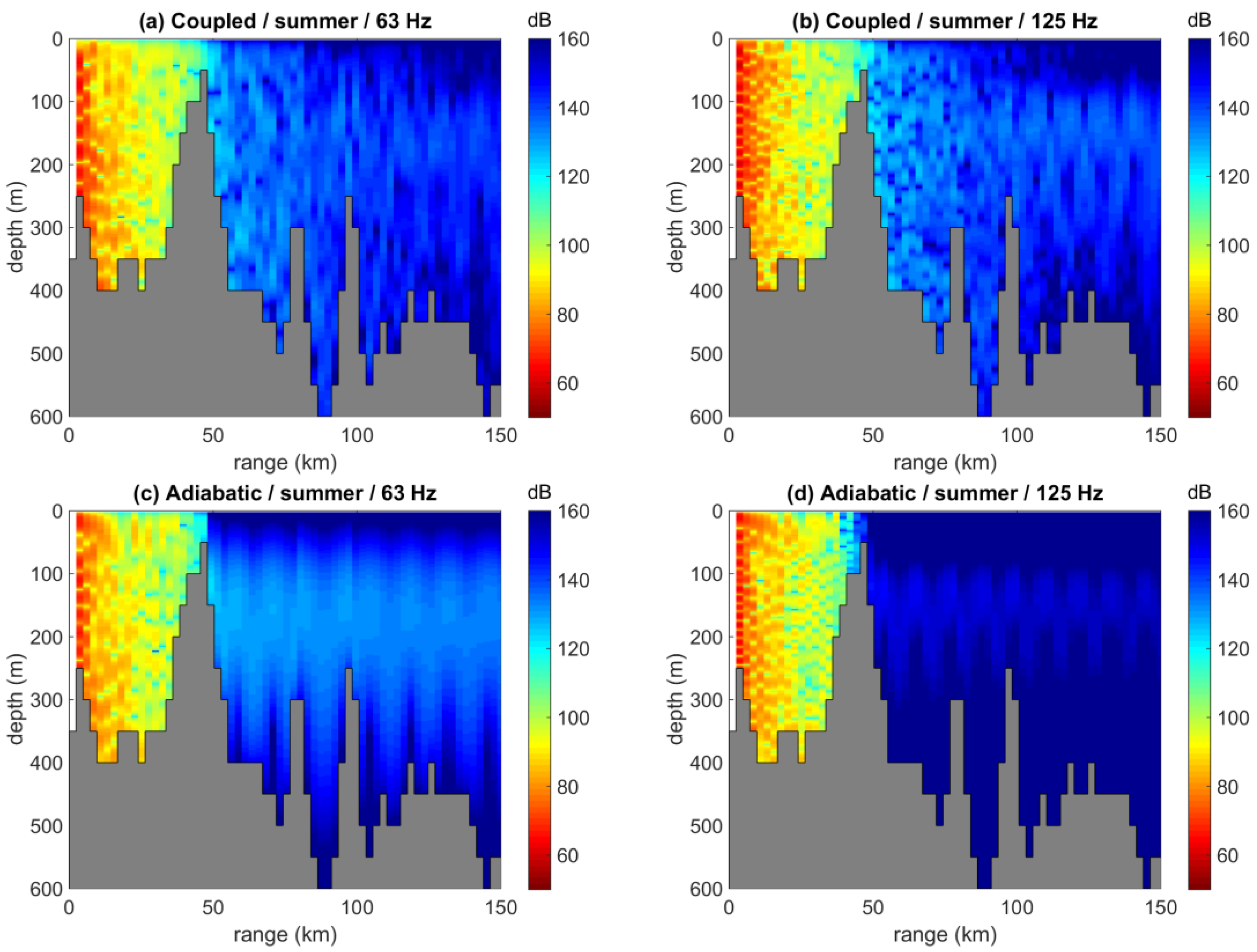
Figure 6 and Figure 7 show the transmission loss (TL) versus range and depth along a nearly 150 km long transect in the Aegean Sea, marked in Figure 3 as AB (see also Table 1), assuming a shallow source at 5 m depth at the northern end (A), using adiabatic and coupled modes at 63 and 125 Hz for the winter and summer SVP, respectively. This particular transect is characterized by strongly range-dependent bathymetry varying between 50 and 600 m, discretized with a step of 50 m. A seamount at the range of 50 km has a blocking effect on the acoustic field at longer ranges, and the effect is stronger in summer than in winter. This is due to the deepening of low-order modes in summer (Figure 5) which are, thus, less efficiently stimulated by the shallow-water source. Because of this, the acoustic field is also somewhat weaker in summer than in winter at shorter ranges. The acoustic frequency also plays a role since the shorter wavelengths associated with the larger frequency of 125 Hz detect the SVP details more efficiently, leading to more intense trapping of acoustic energy in the surface duct in winter at 125 Hz than at 63 Hz, and, thus, to weaker influence by the shallow bathymetric features. On the other hand, since the concentration of acoustic energy about a larger depth, the axial depth of 100 m, i.e., is closer to the bottom in summer, the bathymetry topology is more influential for the propagation. Finally, the comparison between the adiabatic and coupled-mode results indicates that the two predictions are close to each other in the near field, but the differences grow larger at longer ranges. This is true especially after the bottom elevation at 50 km, where, depending on frequency and depth, the adiabatic prediction overestimates or underestimates the acoustic field. The aforementioned results are in good agreement with the ones presented in a report of the QUIETSEAS project for a nearby transect, using the adiabatic and coupled-mode versions of the KRAKENC code [48]. This report contains a comparison of standard normal-mode, parabolic-approximation and ray-theoretic approaches for single-transect TL calculations in various environments in the Mediterranean and Black Sea and for various frequencies, and presents the merits of each approach, also covering issues associated with the computational burden.

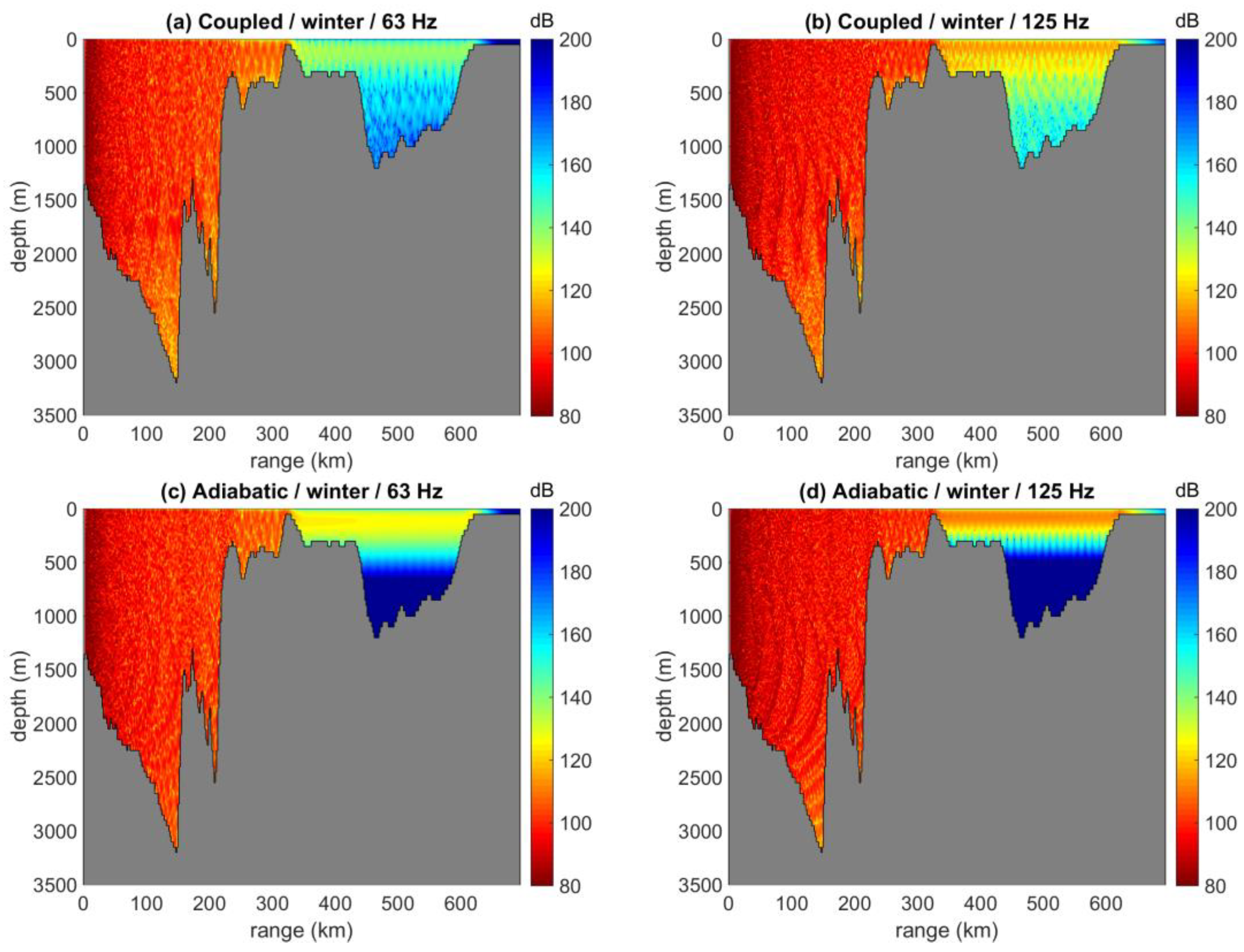
Figure 8 and Figure 9 show TL results along a nearly 700 km long transect in the Ionian Sea (CD transect in Figure 3, Table 1) assuming a shallow source (5 m depth) at the northern end (C). Again, this transect is characterized by strongly range-dependent bathymetry, starting with deep water, depth above 1500 m for the first 200 km, followed by much shallower water towards the south, including a shallow of 50 m at about 300 km range. As in the previous case, the acoustic field in winter is stronger than in summer due to the more efficient stimulation of low-order modes by the shallow source. After the shallow at 300 km, the coupled-mode calculation in winter predicts an acoustic field reaching the largest water depths of 1200 m, whereas the adiabatic calculation predicts a stronger acoustic field, which is, however, confined in the upper 500 m. This is because the coupled-mode calculation, unlike the adiabatic approximation, allows for energy exchange between modes and, thus, for repopulation/revival of higher-order modes extending to larger depths through energy transfer from low-order ones. The deepening of the low-order modes in summer causes an even weaker acoustic field after the shallow at 300 km range, where the adiabatic prediction is characterized by smaller transmission losses.

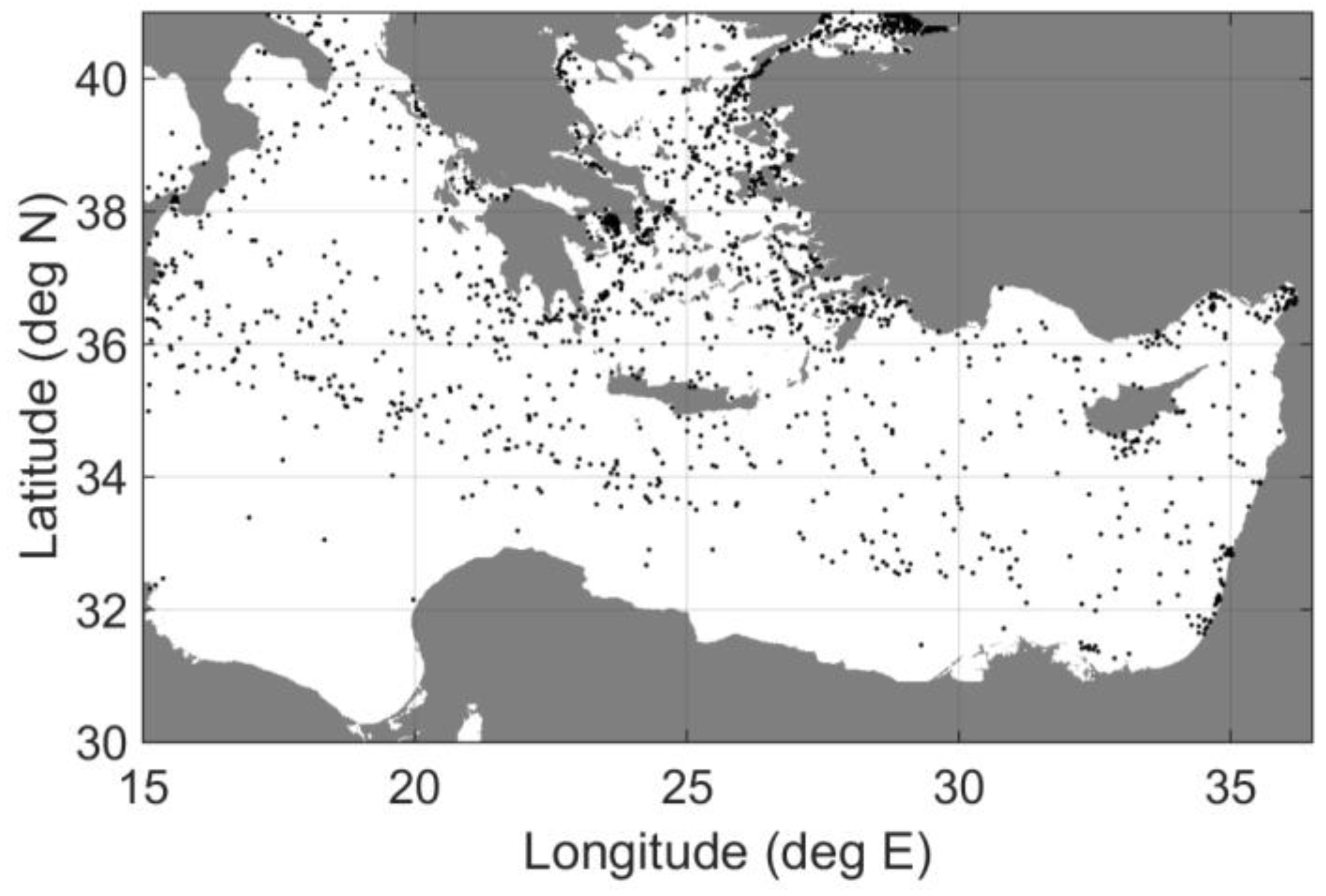
In the following, calculations of the noise field generated by a typical distribution of noise sources (1721 ships) in the Eastern Mediterranean Sea, shown in Figure 10, are carried out. Main shipping routes connecting the Strait of Sicily with the Adriatic Sea, the Aegean and Black Sea, and the Suez Canal can be recognized in Figure 10. All noise sources are assumed to be at a depth of 5 m and to have spectral emission levels of 165 dB re 1 μPa²/Hz @ 1 m at 63 Hz and 155 dB re 1 μPa²/Hz @ 1 m at 125 Hz, following the typical decreasing behavior of acoustic signatures [30]. Nearby acoustic sources are grouped and assigned to the closest grid point and the emission levels are accumulated. Then, the acoustic field of each grouped noise source is calculated along eight transects in the N, NE, E, SE, S, SW, W and NW directions, for locations other than the location of the source, and the results are interpolated in the azimuthal. The acoustic field of the grid point on which the acoustic source is located is assigned the intensity at a range equal to half grid spacing assuming spherical spreading. Increasing the number of transects would improve the azimuthal coverage at the cost of a heavier computational burden.

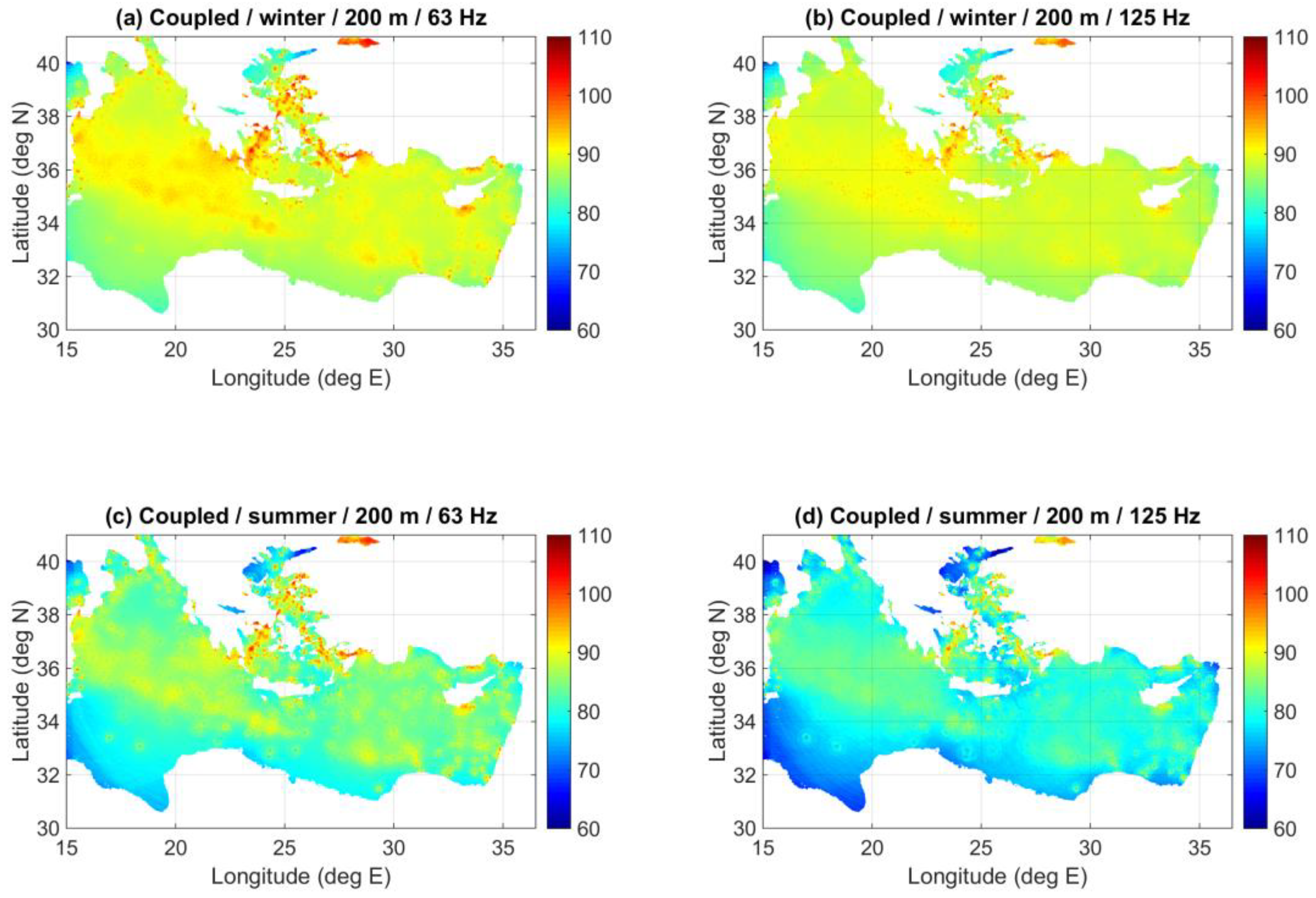
Figure 11 and Figure 12 show the predicted noise field and the spatial distribution of received noise levels (in dB re 1 μPa²/Hz) from the coupled-mode and adiabatic calculations, as well as the difference between the two at a depth of 50 m for the frequencies of 63 and 125 Hz for the winter and summer SVP, respectively. In general, the adiabatic approximation leads to slightly overestimated noise levels, with the differences being largest in areas of changing bathymetry away from the main shipping lanes, e.g., in the south Ionian Sea. This is reasonable, considering that the effect of range dependence cannot be sensed in the vicinity of a source but rather at a distance. It is noted that the noise field at 125 Hz in summer is weaker than at 63 Hz; this is due to a combination of the lower spectral source levels and the larger TL. In winter, the TL is smaller and the two effects nearly cancel out.

Regarding the seasonal effect, it is seen that, for the summer SVP, there is an overall drop in the received noise levels throughout the basin. This is due to the weak stimulation of low-order modes by the shallow-water source, as explained before, which leads to larger transmission losses. Consequently, the acoustic field of the individual noise sources is more localized in summer, revealing the actual source locations, especially in the coupled-mode prediction. In this context, likewise, the differences between the coupled-mode and adiabatic predictions are somewhat more concentrated (less diffused) compared with the corresponding differences in winter (Figure 11). In addition, the differences between the coupled-mode and adiabatic predictions in summer appear to be larger than those in winter. This is possibly due to the fact that the acoustic energy is trapped at a larger depth (the axial depth) in summer compared to that in winter, where bathymetry, range dependence and coupling all have larger influence.

Figure 13 shows coupled-mode predictions of the received noise levels at a depth of 200 m, due to the same ship distribution, at 63 and 125 Hz and for the winter and summer SVP, respectively. Comparison of the corresponding results at a depth of 50 m, Figure 11a,b and Figure 12a,b, respectively, reveals only minor differentiations of the noise field with respect to depth.

The shipping noise predictions presented above are based on propagation calculations from each source along azimuthal transects without any range limitation, i.e., the propagation calculations along each transect are carried out up to the range where land is encountered (water depth goes to zero). The range limitation in the propagation calculations is a common way to reduce the computational burden, especially when (computationally time-consuming) parabolic approximation models are used; in this case, the propagation calculations are carried out up to a range $R_{\max }$ from each source, after which the corresponding acoustic field is truncated. However, this limitation has an effect on the estimated noise levels.

To demonstrate this effect, coupled-mode calculations of the noise field at 63 Hz and 50 m depth were performed using the same source distribution and the same winter/summer SVPs as before, by applying a range limitation of 200 km and 300 km, respectively. The simulation results are presented in Figure 14. By comparing Figure 14a,b with Figure 11a, which describes the prediction without range limitation, it is apparent that the range limitation leads to a significant reduction in the predicted noise levels for the winter SVP. The same outcome can be observed when comparing Figure 14c,d with Figure 12a, corresponding to the predicted noise fields for the summer SVP.

To make the comparison clearer, the differences between the predictions with unlimited propagation range and those with truncated range are presented in Figure 15. As expected, the shorter the limiting range, the larger the differences. Nevertheless, even with a truncation at 300 km, there are significant differences reaching and exceeding 8 dB (up to 20 dB, colored dark red) away from the major shipping lanes, e.g., in the southwestern part of the Ionian basin; note that the color scale in Figure 15 focuses on differences up to 8 dB in order to better illustrate the differences in all marine areas of the entire modelled domain, and larger differences are cropped. Further, the differences are, in general, somewhat larger in winter than in summer. This is associated with the higher noise levels in winter compared to summer, for the same noise source distribution, cf. Figure 11a and Figure 12a, and is an indicator that shipping noise in winter survives longer distances than in summer due to the existence of the surface duct.

4. Discussion and Conclusions

A prediction model for shipping noise in range-dependent environments based on coupled-mode theory has been described. The proposed approach involves precalculation and storage of modal information for a set of local environments spanning the variability in the area of interest, as well as precalculation and storage of coupling matrices between local environments of subsequent discrete water depths. The limitation to consecutive depths, i.e., the avoidance of calculating and storing the coupling matrices between all possible combinations of water depths, reduces the computational burden and storage requirements significantly. Then, for the evaluation of the acoustic field, in cases of abrupt bathymetry changes, additional nodes are introduced and depth interpolation is performed, resulting in range segments of subsequent discrete depths for which coupling matrices are available.

The proposed scheme is used to make noise predictions and elucidate the influence of propagation conditions, frequencies of interest and range limitations on the noise distribution. The noise levels exhibit very small variability with receiver depth, and they are, in general, larger in winter than in summer for the same noise source (ship) distribution. This is because, on the one hand, the noise sources due to shipping are shallow (5–10 m) and, on the other hand, the (low-order) modes are deeper in summer than in winter (due to the larger depth of the channel axis). This causes stronger stimulation of low-order modes in winter than in summer. The higher-order modes are efficiently stimulated in summer since they extend towards the surface, but they are bottom-interacting too, which means that their energy suffers significant bottom losses. As a consequence, the noise level in summer is lower than that in winter. The effect is intensified with increasing frequency, i.e., the high noise levels in winter become higher with increasing frequencies, whereas the low noise levels in summer become lower with increasing frequencies. This happens because the shorter wavelengths, corresponding to the higher frequencies, follow the SVP details more closely, leading to propagating modes supported even closer to the surface at higher frequencies in winter and even further away from the surface at higher frequencies in summer.

It should be mentioned here that the predicted noise levels are substantially influenced by the depth of the noise source. Since the propagating modes vanish at the surface, their stimulation by a shallow source, and, thus, the induced acoustic field, depends on the source depth. Numerical results demonstrating this effect are beyond the scope of the present paper and are going to be part of a future work. Taking into account that cavitation, the primary ship noise-generation mechanism, is strongest on the propeller blades closest to the surface, the noise source should be placed in the upper propeller half, above the propeller shaft and probably close to the top of the propeller. Unfortunately, the propeller diameter, which, together with the ship draught, could provide an estimate for this depth, is not included in the static AIS data, which means that the source depth remains a source of uncertainty.

As regards the comparison between the adiabatic and the coupled-mode prediction, in general, the former leads to slightly overestimated noise levels, and the differences are larger in summer than in winter. This is because the summer SVP traps the acoustic energy about a larger depth (axial depth) and, thus, causes it to interact with the bottom (to ‘feel’ the bathymetry) more strongly. Additionally, the differences are observed mostly far away from the noise sources (shipping routes) rather than close to them. This can be explained by the fact that the adiabatic approximation is not expected to deviate from the coupled-mode solution at short distances from a source but rather at larger distances, where the effects of range dependence on propagation become significant. Finally, in environments with abrupt bathymetry changes from shallow to deep water, such as in the case of the transect CD, the adiabatic prediction is expected to perform poorly when coming to the deep-water part, since it cannot repopulate higher-order modes. This gives an additional argument for the use of coupled modes in areas of complicated bathymetry.

The computational cost of the coupled-mode evaluation of the acoustic field over the Eastern Mediterranean Basin following the proposed approach for the cases considered has been found to be 8–10% larger than that of the adiabatic approximation. This increase is mainly due to the introduction of additional range segments and the recurring calculation of the acoustic field within each new range segment using the coupling matrices. More specifically, to properly calculate the acoustic field, this scheme requires the introduction of additional grid points in areas of abrupt depth changes such that the differences between depths of adjacent range segments equals the depth resolution. On the other hand, the choice to limit mode coupling only when the bathymetry changes at subsequent grid points reduces both the computational cost and the storage requirement and complexity.

A common way to reduce the computational burden of the noise predictions is to apply range limitations in the propagation calculations, i.e., truncate the acoustic field of each noise source at a certain maximum range. However, such a limitation may lead to significant underestimation of the shipping noise footprint, as shown in the previous section, especially in marine areas away from main shipping lanes. In the absence of other noise-generating anthropogenic activity, the significance of this underestimation for a particular area depends on the noise level from natural sources, such as wind, waves and rain. In general, in order to assess the significance of the differences in the shipping noise prediction associated with parameter selections (source depth, cutoff range, etc.) or model assumptions (e.g., adiabatic vs. coupled-mode approach), the natural background noise should be accounted for. Thus, depending on the expected natural noise background, some of the finer differences might be actually obscured in practice, particularly in areas of low ship traffic away from main shipping lanes.

Although the range dependence of the environment in the examples presented here is only with respect to bathymetry, the proposed method can cope with spatially variable bottom and water-column characteristics as well. These can result from cluster analysis of available temperature and salinity data, e.g., from oceanographic models or measurements, and geological information. Such an analysis is currently underway, aiming to upgrade the existing noise-prediction model for the Eastern Mediterranean Sea, which is based on AIS data and adiabatic propagation modelling [49], by using better environmental data and a more complete propagation model.

Last but not least, it should be stressed that a further necessary step towards the development of a reliable shipping noise-prediction model is the comparison of model predictions with medium- to long-term measurements at selected locations. While models can reveal the sensitivity of the noise field with respect to parameters such as the depth of the noise sources and the propagation conditions, a series of dedicated noise measurements will allow for model assessment and calibration to establish a firm basis in support of relevant decision-making systems. The anticipated intensification of noise measurement campaigns in the Eastern Mediterranean Sea in the years to come, combined with advancements in the noise-prediction modeling (to result from better monitoring of marine traffic, reliable acoustic characteristics of ships, realistic environmental data and efficient propagation modelling) is expected to pave the way for meaningful comparison studies.