Feature-Based Place Recognition Using Forward-Looking Sonar

Abstract

Some structures in the harbour environment need to be inspected regularly. However, these scenarios present a major challenge for the accurate estimation of a vehicle’s position and subsequent recognition of similar images. In these scenarios, visibility can be poor, making place recognition a difficult task as the visual appearance of a local feature can be compromised. Under these operating conditions, imaging sonars are a promising solution. The quality of the captured images is affected by some factors but they do not suffer from haze, which is an advantage. Therefore, a purely acoustic approach for unsupervised recognition of similar images based on forward-looking sonar (FLS) data is proposed to solve the perception problems in harbour facilities. To simplify the variation of environment parameters and sensor configurations, and given the need for online data for these applications, a harbour scenario was recreated using the Stonefish simulator. Therefore, experiments were conducted with preconfigured user trajectories to simulate inspections in the vicinity of structures. The place recognition approach performs better than the results obtained from optical images. The proposed method provides a good compromise in terms of distinctiveness, achieving 87.5% recall considering appropriate constraints and assumptions for this task given its impact on navigation success. That is, it is based on a similarity threshold of 0.3 and 12 consistent features to consider only effective loops. The behaviour of FLS is the same regardless of the environment conditions and thus this work opens new horizons for the use of these sensors as a great aid for underwater perception, namely, to avoid degradation of navigation performance in muddy conditions.

1. Introduction

Harbour facilities include various structures such as quay walls and adjacent piles that need to be inspected for corrosion and damage. The inspection of these structures is normally carried out by divers and remotely operated vehicles (ROVs). However, this work is dangerous and ROVs use a cable that can restrict and complicate work in these semi-structured environments. Therefore, autonomous underwater vehicles (AUVs) have been used for these tasks. To perform an inspection, they must accurately navigate and recognise revisited places, also known as loop closure detection, to compensate for cumulative pose deviations [1]. In an image-only retrieval model, the decision of whether the sensor has reached a revisited scene during its movement is based on similarity measures between images stored on maps. However, due to perceptual limitations, navigation near structures is still a challenge. Deep learning is a powerful technique that is increasingly used in this field of research [2,3]. However, it requires a large amount of data and a long training phase, which is a complex task in these semi-structured and unknown scenarios. On the other hand, traditional machine learning techniques focus on identifying previous observations, which makes the navigation principles very stationary and dependent on the representativeness of the collected observations. Although it is challenging to make this decision independently of the environment, i.e., through unsupervised learning, it is important that the vehicle continuously learns the environment during the inspection mission in order to adapt its behaviour accordingly. Vision-based systems are an attractive environmental sensing solution for robust close-range operations because they work at distances of less than 3 m (metres), provide rich information and are easy to operate [4]. However, the underwater environment is dynamic and lacks structural features. In addition, this environment is often affected by turbidity or illumination (shallow waters), which often complicates the behaviour of navigation and mapping tasks performed by cameras, as the perception range of optical devices is severely limited in very poor visibility. Such conditions make the detection of loop closures difficult, and the vehicle may fail to detect some loops correctly or detect some erroneous loops so that the trajectory is not adjusted or adjusted incorrectly. In a previous study, the efficiency of a purely visual system for recognising similar images was analysed. This analysis showed that cameras are susceptible to strong haze and brightness conditions, achieving at best a 71% detection rate, even with enhancement techniques that provide more consistent keypoints [5]. Today, there is a new type of sonars (SOund Navigation And Ranging) known as active sonars. They can emit an acoustic wave and receive the backscatter, so they provide acoustic images that allow them to perceive the environment, i.e., they are also called imaging sonars [6]. Although these sensors suffer from distortion and occlusion effects due to their physical properties, they do not suffer from haze effects as the images are based on the emitted and returned sound. Therefore, this category of sonar is seen as a promising solution for these difficult environment conditions. Forward-looking sonar (FLS) and side scan sonar (SSS) are the most commonly used sonars for environment sensing. FLS is characterised by the fact that it provides a representation of the environment in front of the robot and allows overlapping images during movement. Image matching is the first problem to solve, as it is the crucial step for pose estimation or place recognition. Due to the characteristics of FLS data, namely, low signal-to-noise ratio, low/inhomogeneous resolution and weak feature textures, traditional feature-based registration methods are not yet used for acoustic images. In her work, Vilarnau [7] proposes a pairwise registration of FLS images for the mosaic pipeline based on a Fourier method that can provide robustness to some artefacts commonly associated with acoustic imaging and noise for all image contents. For the inspection of ship hulls with FLS images, a machine learning method for the detection of loop closures based on saliency was used in 2018. To deal with the sparse distribution of sonar images, it is based on the evaluation of the potential information gain and the estimated saliency of the sonar image [8]. Later, a loop closure detector was proposed for a semi-structured underwater environment using only acoustic images acquired by an FLS [9]. A topological relationship between objects in the scene is analysed based on a probabilistic Gaussian function. It is based on regions with higher acoustic intensity variations, i.e., segments. The method achieves a precision of 95.38% at best and a recall of 12.24%, which is dangerous for the navigation context as there are some false trajectory adjustments and also many adjustments fail. But the performance of these sonars has greatly improved and the resolution of their images continues to increase so that the FLS can provide comprehensive underwater acoustic images. Therefore, developing efficient approaches to extracting visual data from sonar images and understanding their performance remains critical to ensure that the FLS data are suitable for the vehicle’s perception of the environment. Furthermore, these data can later be matched with the camera data if required as environment conditions change. The matching algorithms can be based on feature points and region approaches, but given the FLS characteristics and real-time constraints of underwater operations, feature point matching is more appropriate. Given the need for viewpoint invariant feature descriptors, binary methods are increasingly being used for similarity detection. These features require less memory and computation time. Proof of this was provided in underwater scenes categorised by seabed features, turbidity and illumination. Here, the Oriented FAST and Rotated BRIEF (ORB) descriptor proved to be more effective for detection and matching with the least computational time [10]. Recently, its behaviour was also demonstrated for acoustic images using a performance comparison of different feature detectors, where ORB achieved the best overall performance [11]. For fast and effective loop closure based on visual appearance, the bag-of-words (BoW) algorithm is often used for data representation. In this approach, the local descriptors are usually clustered using the K-Means technique and a codebook of visual words is required. Each local descriptor is assigned to the nearest centroid and the representation is in the form of a histogram. Its efficiency through inverted index file and hierarchical structures is favourable [12,13].

In short, the inspection of some underwater structures is crucial but still a challenge as the vehicles need to perceive the environment and get close to the object that is to be inspected. Place recognition or loop closure detection is an important task to enable successful navigation while compensating for cumulative deviations in pose estimation. But it is also a challenge as it requires the effective identification of previously seen landmarks. Typically, visibility conditions in such underwater scenarios are poor, so FLS can be a promising solution for robust loop closure detection. There are some inherent problems that make it difficult to continuously perceive a vehicle’s surroundings, such as the low and inhomogeneous resolution, which affects the visual appearance of images with weak feature textures. In addition, inhomogeneous insonification associated with the angle of incidence or tilt can also lead to occlusion-related shadows and significant changes in visual appearance, especially in semi-structured environments. However, these sensors can also be used in cloudy environments.

Therefore, this paper proposes a feature-based place recognition using only the sonar images captured by FLS. The loop closure decision is based on a continuous learning approach, i.e., an unsupervised machine learning technique, so that the scenes are continuously modelled during the mission. The idea is to apply the knowledge of the visual to the acoustic data to evaluate whether it is effective in detecting loops at close range, and then utilise its potential in conditions where cameras can no longer provide such distinguishable information. To facilitate the variation of environment parameters and sensor configurations, and given the lack of online data to fulfil the requirements in this context, a harbour scenario based on the Stonefish simulator [14] was recreated.

The most important contributions of this work therefore include:

• An evaluation of the effectiveness of extracting visual data, i.e., features from sonar images;
• An understanding of the needs and behaviour of sonar deployed in the vicinity of structures;
• An evaluation of a proposed visual approach to place recognition from sonar data.

The paper is organised as follows: Section 2 describes the FLS basics and the Stonefish simulator used to capture underwater images and replicate real-world conditions. Section 3 describes the proposed algorithm for place recognition based on forward-looking sonar data. Section 4 describes in detail the performance metrics used. In addition, both the evaluation of the image description and matching techniques and the behaviour of the already-seen places for the different experiments performed are presented in detail. Finally, Section 5 describes the main conclusions and planned next steps of this work.

2. Background

In most cases, sensors normally used for outdoor navigation and mapping pose several challenges when used in an underwater environment. Underwater turbidity, poor lighting conditions and particles in the water make both visual and laser-based range sensors useless. Nevertheless, the vehicles must be able to recognise their surroundings. Attention is therefore turned to sonars, as sound propagates well in water and can travel thousands of metres without losing energy, even in murky water. Active sonars, namely, FLS, allow monitoring of the environment by generating an image of the scene in front of the robot with each scan. Therefore, it is important to understand the basics of FLS before we move on to the different steps of the place recognition pipeline.

Therefore, Section 2.1 describes the working principles of FLS devices, the generation of acoustic images and the main challenges in handling FLS images that may affect subsequent processes such as image matching and consequent decisions to close the loop. In addition, Section 2.2 introduces the Stonefish simulator that is used to replicate the intended scenario, which includes some environment parameters and the selected FLS geometry model.

2.1. Forward-Looking Sonar

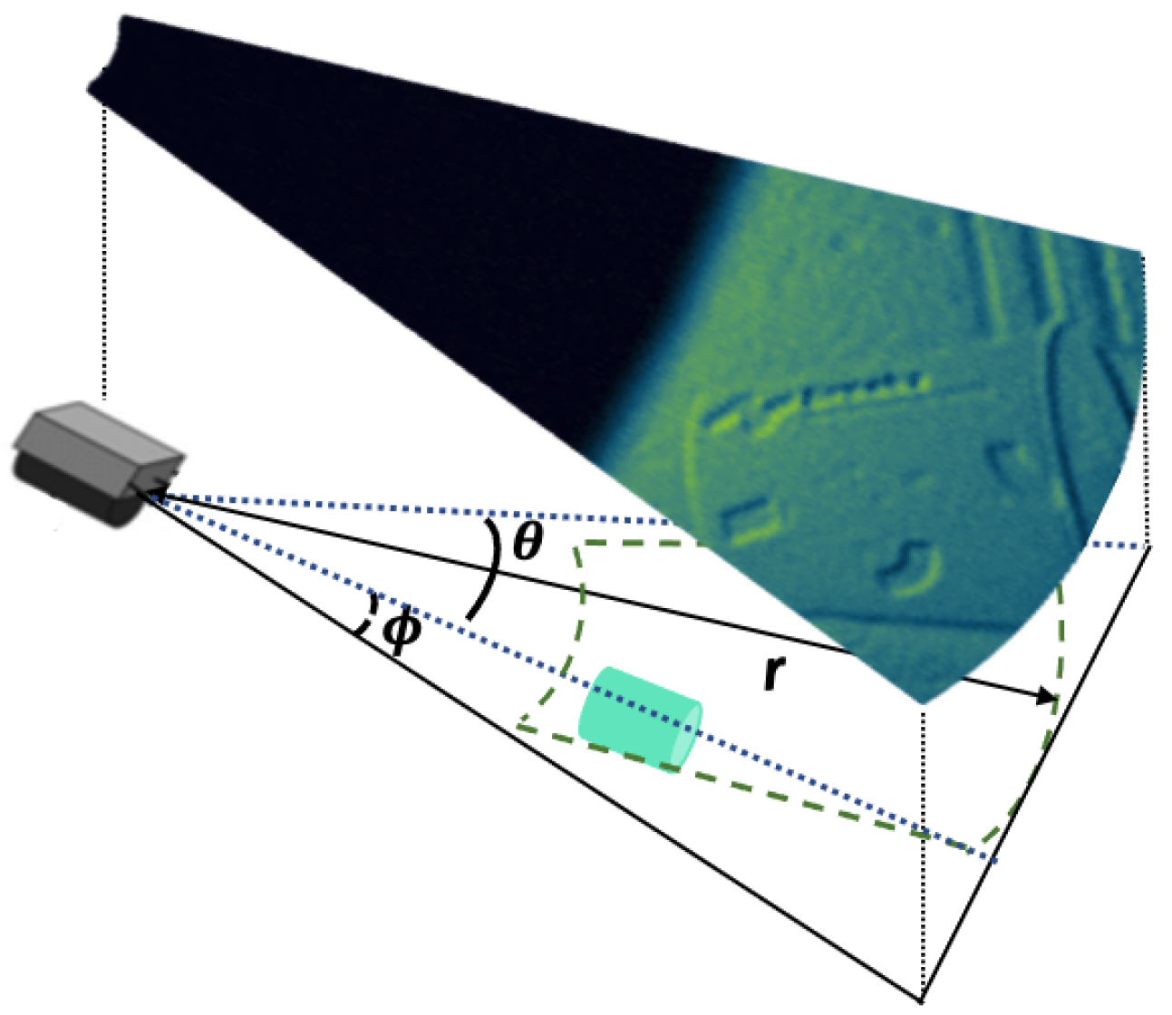
The two-dimensional (2D) FLS is a new category of sonar that can provide acoustic images at a high frame rate and is therefore also referred to as an acoustic camera. The various operating specifications, such as acoustic beam width, operating frequency, acquisition rate and beamforming, are always associated with the sensor models. However, the operation of sonars remains the same: the sonar emits acoustic waves that cover its field of view (FOV) in azimuth ($\theta$) and elevation ($\varphi$), and the intensity of the returning beam is then determined based on a range (r) and bearing ($\theta$), as shown in Figure 1.

FLS imaging projects a 3D scene into a 2D image, just like an optical camera; the depth of objects is not lost but on a sonar image it is not possible to uniquely determine the elevation angle at a given r and $\theta$, i.e., the reflected echo can originate from any point in the reference elevation arc. The images are arranged and mapped in polar coordinates. In this way, the measurements of a raw image correspond to the beams in the angular direction and the range samples in the distance axis. For easier interpretation, the resulting image is then mapped to two-dimensional Cartesian coordinates, resulting in images with uneven resolution. Acoustic images are able to see through murky environments, but at the cost of a much more difficult type of data. Therefore, there are some issues associated with this type of sonar imagery that can be challenging for inspection tasks, such as:

• Low resolution: Although FLSs are often categorised as high-resolution sonars, their image resolution falls far behind that of modern cameras, which typically have millions of pixels. Of course, the resolutions in the cross and down range are crucial for image quality and for distinguishing between closely spaced objects. However, the sparseness of the measurements increases with distance when they are displayed in Cartesian space. This leads to uneven resolution, which affects the visual appearance of images with weak feature textures;
• Low signal-to-noise ratio: Even with a large FOV, sonar images have a high noise level due to mutual interference from sampled acoustic echoes, underwater motors near the surface or other acoustic sensors;
• Inhomogeneous insonification: FLSs usually have a Time Varying Gain (TVG) mechanism with the aim of compensating for transmission losses so that similar targets located at different distances can be perceived with similar intensity. However, changing the angle of incidence or tilt can lead to variations in image illumination and other effects that depend on the varying sensitivity of the transducers or lens, which in turn depends on their position in the sonar’s FOV. These inhomogeneous intensities can influence the image matching step and, of course, the pose estimation and loop closure phases. It is recommended to configure the forward-looking sonar so that there is a small angle between the imaged plane and the bore line (grazing angle), as this allows the largest possible volume [15]. Of course, a small angle results in a larger area with no reflected echoes in the image (black area), reducing the effective imaging area, but this configuration allows the vehicles to perform inspection tasks for structures that require close-range navigation. This is due to the fact that it also avoids shadows in the images caused by occlusions and significant changes in visual appearance;
• Other artefacts: Interfering content can appear in the sonar images, which can lead to ambiguities during matching: acoustic reflections from the surface, artefacts due to reverberation or ghost artefacts. However, these interferences can usually be reduced by a suitable configuration and image composition.

2.2. Stonefish Simulator

For an initial evaluation of the feasibility of using FLS images to recognise visited places, the Stonefish simulator was used. Its main goal is to create realistic simulations of mobile robots in the ocean, taking into account the effects of scattering and light absorption. It is an open-source C++ library that makes it possible to change the position of the sun in the sky, simulate optical effects in water and also take into account the effects of suspended particles. In addition, it is possible to create specific scenarios, including one where so-called “static bodies” remain fixed at the origin of the world for the entire duration of the simulation; they are typically used for collision and sensor simulations. Static bodies include a simple plane, simple solids (obstacles), meshes and terrain.

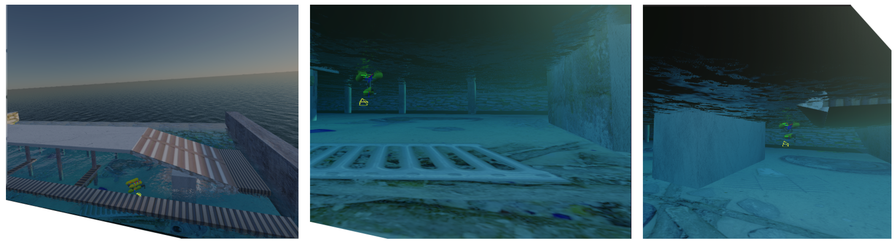
Therefore, a harbour scenario is recreated to simulate inspection operations in port infrastructures that replicate various structures: quay walls, piers and pillars, i.e., a berth area. The ground is also simulated and consists of some objects commonly found in harbour facilities, such as garbage, amphorae, anchors and metal grids. Figure 2 shows a wide view of the scenario of the simulated harbour facilities.

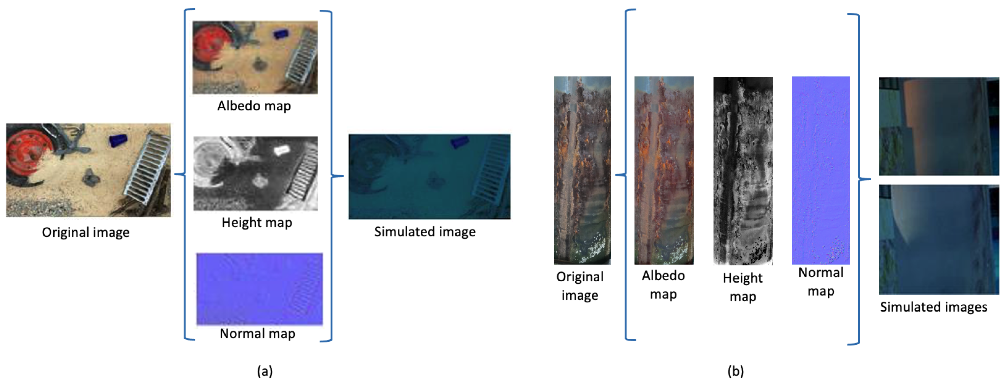
To create the real look of the structures and the seabed, a graphical material called “looks” must be created, which defines how the objects are rendered. All looks are parameterised by reflectance (colour), roughness, metallicity and reflection factor (0 for no reflection to 1 for mirror) to get a real simulation of the echoes returned by the sonar. All structures as well as the bottom are considered as rock (material) with a certain roughness and thus without metallicity factor and without reflections. To add texture to a material, both albedo and normal (or bump) maps are created based on original images to represent the appearance or texture of the scenes. Figure 3 illustrates the entire rendering process described. The correct setting of the individual maps is crucial for successful rendering, especially the strength of the bump map. By default, the visibility conditions caused by turbidity (called “waterType”) and the sun orientation (called “SunPosition”) are set so that the simulated scenario looks sufficiently realistic, i.e., without strict visibility conditions.

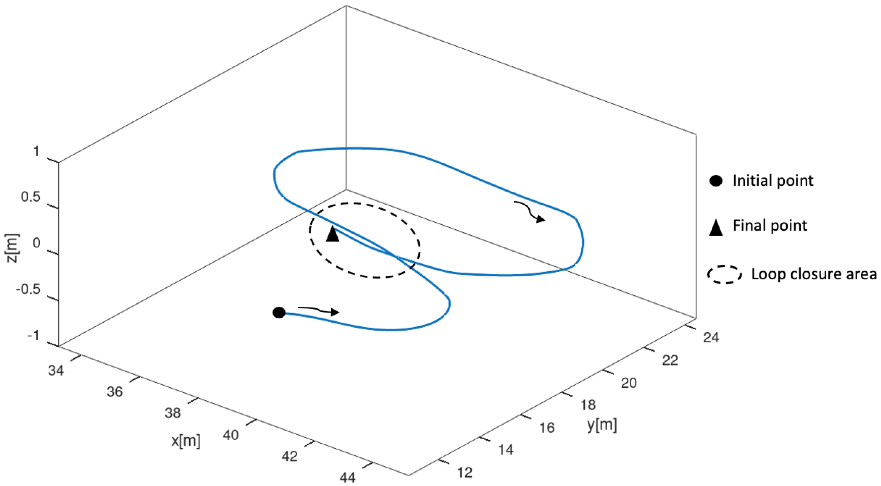
The simulated AUV—Girona 500—autonomously executes predefined trajectories between different waypoints. Thus, taking into account the propulsion system of Girona 500—five thrusters—a state machine was designed for the AUV to perform an appropriate motion according to the required control motion—e.g., straight ahead or change of direction, with a certain force for a smooth navigation to collect reliable data, but also sufficient to react to the difficulties of the underwater environment (waves, currents, wind, etc.) and even the payload of the vehicle. In this context, an FLS and an odometry sensor (ground truth data) were installed on the vehicle. Both sensors were set with an acquisition rate of about 7 Hz. To simulate a mission operation, a trajectory near structures (the vehicle moves about 2–3 m away from the structures) was performed by the AUV at a fixed height, with z set as default. The trajectory has a closed loop as the robot travels around the concrete wall and maintains the view angle as shown in Figure 4. It moves at a speed of 0.65 metres/second (m/s) and reduces its movement speed by 0.25 m/s as it approaches a certain waypoint. If the AUV needs to change its direction of movement to reach an intended waypoint, it turns at 0.4 m/s.

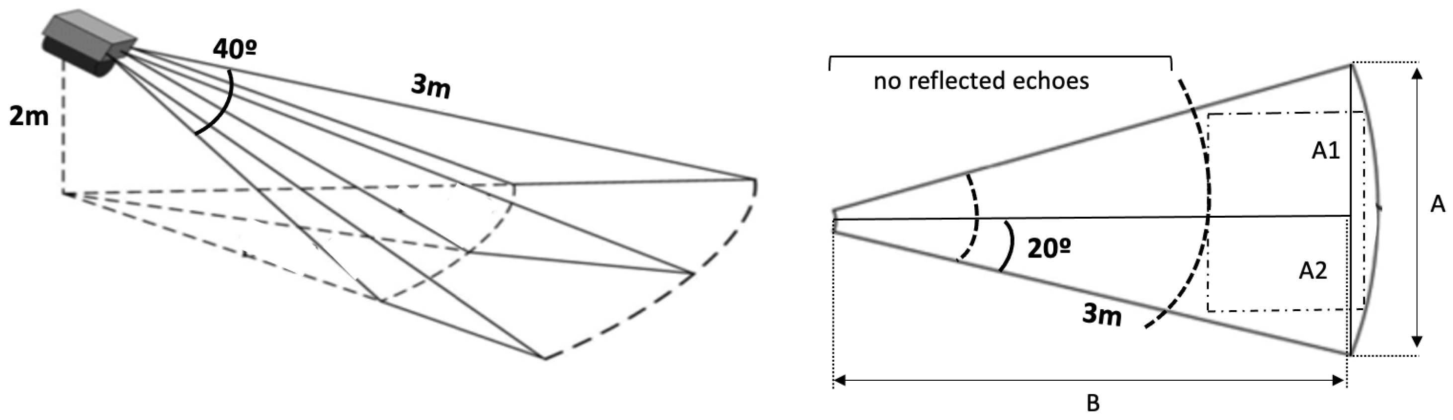
The FLS is a top-down sensor, and as it is intended to provide data about the ground close to the structures under inspection, its design and configuration have been adapted accordingly. It has been configured for a range of up to 3 m (maximum measured range) at a constant standard height of 2 m above the seabed. To create good imaging conditions, the sonar was tilted by 35° and had a horizontal FOV of 40°. In addition, the sonar measurements have 512 beams and 750 bins (range resolution of the sonar image) to mimic the Gemini 720ik sonar (Tritech International Limited, Westhill, Aberdeenshire, United Kingdom) that will be used later for real tests. Thus, each sonar image consists of 514 × 720 pixels. A total of 1067 images are taken during the trajectory of the mission. Once the simulation is complete, the images and the pose for each image are saved in a folder and in a text file. 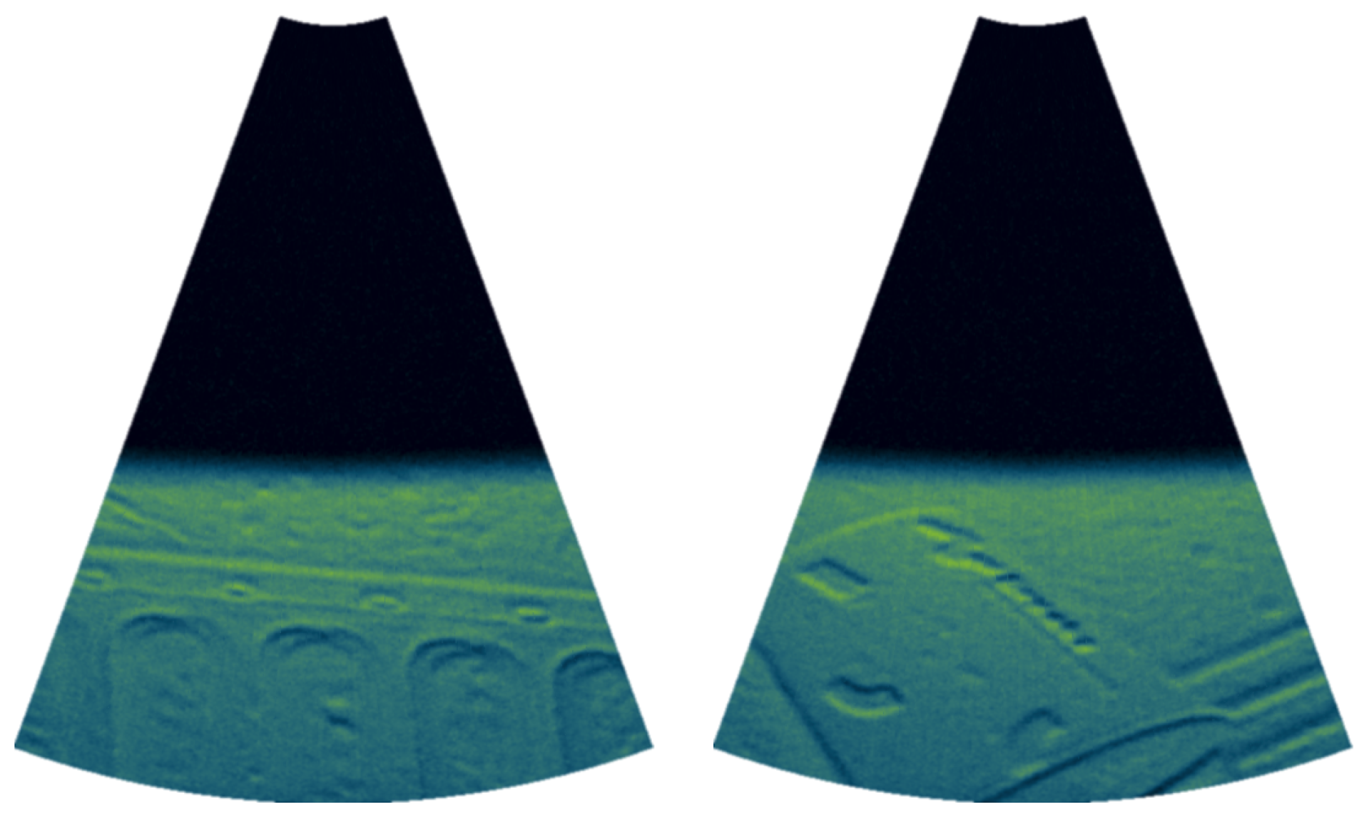Figure 5 shows an example of the output of the sonar images.

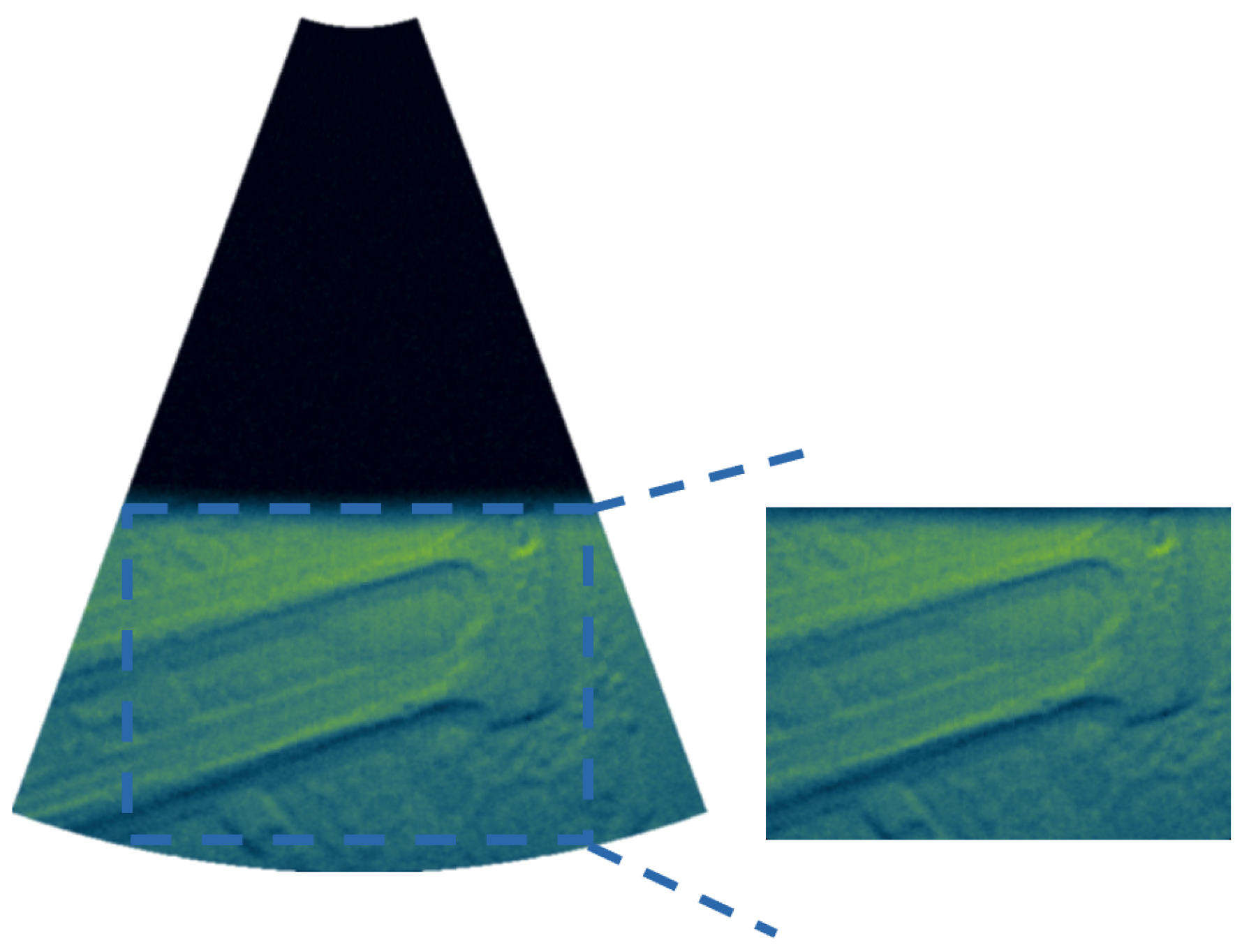
Based on the geometry model schematically shown in Figure 6, each FLS image covers a width of about 2 m (A) and a height of 3 m (B), i.e., it represents an area of about 6 m². However, there is an area without reflected echoes, which is shown as a black area in Figure 5. Therefore, for each FLS image, a region of interest (ROI) is selected to represent the effectively imaged area of the FLS output. Thus, a bounding box of 250 × 350 pixels is used, which means that each FLS image maps an area of approximately 1.5 m², as shown in Figure 7.

3. Acoustic-Based Place Recognition

In practise, place recognition is used to search an image database for images similar to a queried image in an image database. It is considered a key aspect for the successful localisation of robots, namely, to create a map of their surroundings in order to localise themselves (SLAM) [16]. This task is therefore also referred to as loop closure and takes place when the robot returns to a point on its trajectory. In this context, correct data association is required so that the robot can uniquely identify landmarks that match those previously seen and by which the loop closure can be identified. A place recognition system must therefore have an internal representation, i.e., a map with a set of distinguishable landmarks in the environment that can be compared with the incoming data. Next, the system must report whether the current information comes from a known place and if so, from which one. Finally, the map is updated accordingly. Since this is an image-only retrieval model, the map consists of the stored images, so appearance-based methods are most commonly used. These methods are seen as a potential solution that enables fast and efficient loop closure detection—content-based image retrieval (CBIR), as this scene information does not depend on pose and consequently on error estimation. So, “how can robots use an image of a place to decide whether it is a place they have already seen or not?”. In order to decide whether an image is a new or not (known) location, a matching is made between the queried and database images using a similarity measure. The extraction of features is therefore the first step in CBIR in order to obtain a numerical description. These features must then be aggregated and stored in a data structure in an abstract and compressed form (data representation) to facilitate the similarity search. These measures indicate which places (image content) are most similar to the current place. This is an important step that affects CBIR performance, as an inappropriate measure will recognise fewer similar images and reduce the accuracy of the CBIR system.

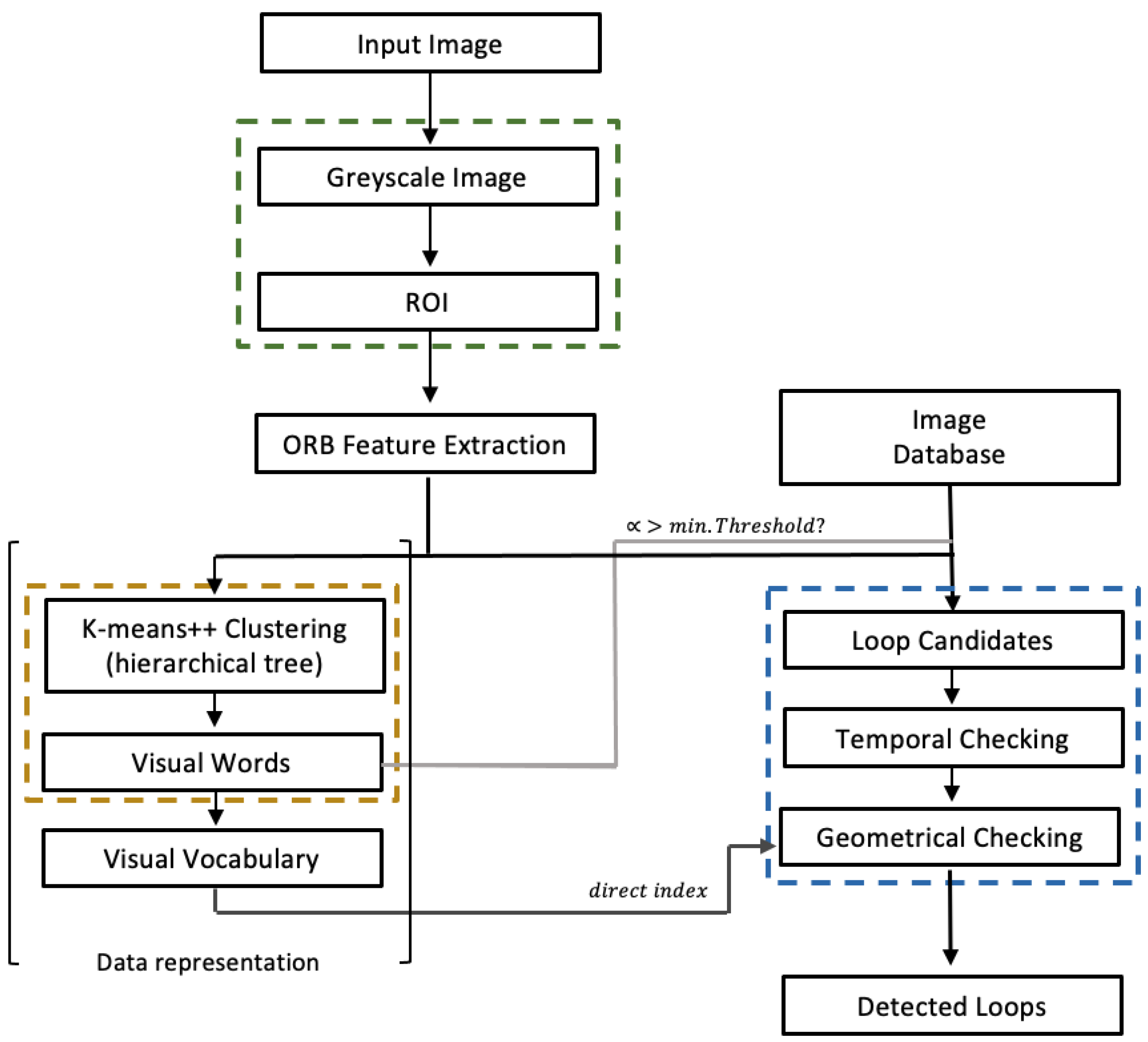
Therefore, a tree-based approach to similarity detection for the intended context is proposed, based on the DBoW21 and DLoopDetector2 libraries [17]. This method was introduced in [5] for optical images and is now adapted for acoustic images. Figure 8 shows the process of place recognition based on FLS images.

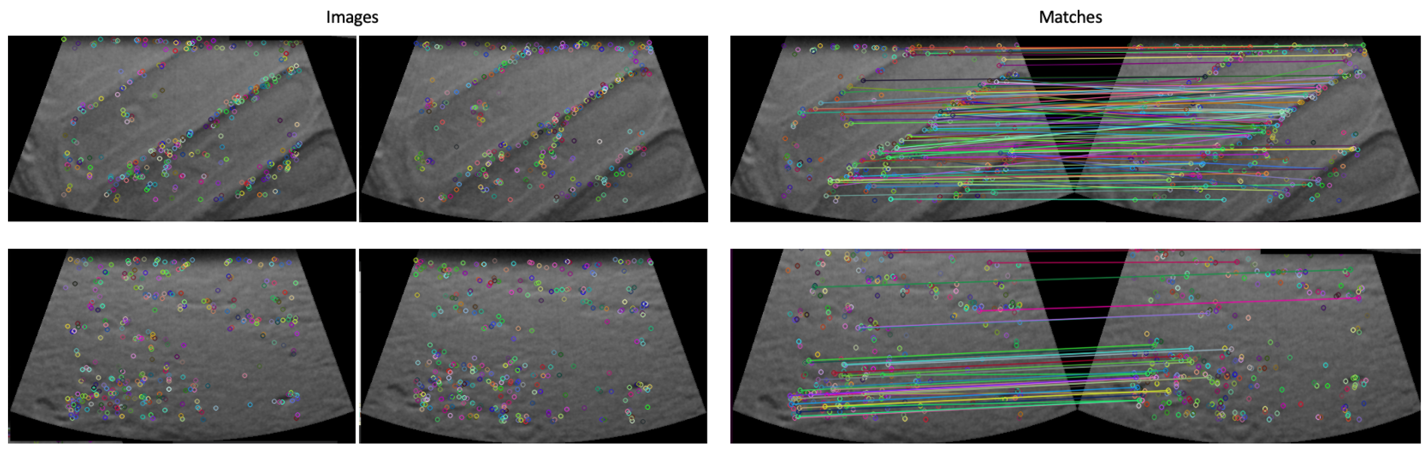
For each current image, an ROI is used to discard the area without reflected echoes. Thus, each input image is “clipped” in a rectangular region to account for the effective visual information captured by FLS, as described in Section 2.2. First, features and descriptors are extracted for each image. In this case, binary features are used, namely, ORB features. As mentioned in Section 1, the binary methods are used because the descriptors for the features must be view invariant. On the other hand, these features require less memory and computation time. Among these methods, ORB stands out as it achieves the best overall performance. More importantly, it proves to be more effective for detection and matching with the least computation time in underwater scenes captured with either cameras covering different environment conditions or acoustic images. It responds better to changes in the scene, especially in terms of orientation and lighting. Based on these features, an agglomerative hierarchical vocabulary is then created using the K-Means++ algorithm; based on the Manhattan distance, clustering steps are performed for each level. In this way, a tree with W leaves (the words of the vocabulary) is finally obtained, in which each word is weighted according to its relevance. Along the BoW, inverted and direct indices are maintained to ensure fast comparisons and queries, and then the vocabulary is stored (yellow block in Figure 8). Next, marked by the blue dashed line, the ROI for each input image is used to recognise similar places, and ORB features are extracted and converted into a BoW vector $v_t$ (based on Hamming distance). The database, i.e., the stored images of previously visited places, is searched for $v_t$ and based on the weight of each word and its score (L1 score, i.e., Manhattan distance) a list of matching candidates is created, represented by the light grey link. Only matches with a score higher than the similarity threshold $\alpha$ are considered. In addition, images that have a similar acquisition time are grouped together (islands) and each group is scored against a time constraint. In addition, each loop candidate must fulfil a geometric test in which RANSAC is supported by at least 12 correspondences, minFPnts. This value is a common default value for comparing two visual images with different timestamps and therefore possibly different perspectives, resulting in a small overlap area compared to consecutive images. These correspondences are calculated with the direct index using the vocabulary represented by the dark grey link.

To measure the robustness of the feature extraction/matching and similarity detection approaches between FLS images, appropriate performance metrics are calculated. Their descriptions can be found in Section 4.1 and Section 4.2.

4. Experimental Results

This section describes the operation of the algorithm for acoustic place recognition in an underwater harbour environment. For this purpose, a dataset with visibility constraints was created using the Stonefish3 simulator to perform the proposed experiments and evaluations. The performance measures used to evaluate ORB on FLS images and their effectiveness are described and illustrated in Section 4.1. In Section 4.2, the performance metrics used to evaluate the detection of binary loop closures are described. Their behaviour when detecting revisited places with different configurations is also shown. An Intel i7 7700K @ 4.5 GHz with 16 GB RAM and an NVIDIA GTX 1080 computer were used for the experiments.

4.1. Acoustic Features Effectiveness

Imaging sonars provide increasingly rich acoustic images that allow us to perceive the environment. However, inherent features such as weak textures, interfering content and low signal-to-noise ratio can affect the subsequent imaging phases, especially feature extraction and matching. Therefore, a functional analysis is considered to analyse the behaviour of the ORB on acoustic images based on the number of ORB keypoints (Kp), the number of matches (Nm) and inliers. The detected Kp on the input images are related to the visual content, as a higher value usually indicates a better description of the scene. Nevertheless, in some situations there may be pixels that are noisy, resulting in incorrectly recognised keypoints. Nm stands for the number of Kp of a query image that correspond to those in the current image, based on the Hamming distance. Finally, the inliers are the correct correspondences between two images. The RANdom SAmple Consenus (RANSAC) from the previously obtained matches [18] is used for this; the higher the value, the more similar the compared images are.

Different textures were tested under standard environmental conditions to analyse the behaviour of feature extraction and matching algorithms on FLS images. All experiments rely on up to 1500 features per image for the extraction step.

Table 1. Functional evaluation for grid and ground areas surveyed with FLS considering standard visual conditions.

		Grid Area		Bottom Area
Functional Evaluation	Kp	326
	Nm	326
	Inliers	90		41

shows the performance evaluation for each scenario. A set of 30 consecutive images is used, with each value determined by a simple arithmetic mean.

As you can see, the descriptor finds the same number of keypoints for grid and bottom areas. However, the effective matches are higher in the grid region, as the bottom region contains only a few stones, an area with low texture. An example of this behaviour for both scenarios can be found in Figure 9, which is illustrated by a high number of linear lines (correct matches).

Table 2. Functional evaluation for grid and ground areas captured by a camera considering standard viewing conditions.

		Grid Area	Bottom Area
Functional Evaluation	Kp	935	332
	Nm	914	313
	Inliers	643	151

shows the obtained functional evaluation considering optical images for both scenarios, based on the same sequence of 30 images. It is evident that optical images have more keypoints and correct matches between consecutive images when visibility is appropriate, as these sensors provide images with more details and have a stronger texture perception, since FLS images are based on emitted and returned sounds.

However, the cameras are sensitive to poor texture scenarios, as shown by the drop in all functional measures (bottom area). Indeed, the performance in such areas was not so far from that obtained with the acoustic images: only three times more instead of seven. Moreover, the FLSs do not suffer from visibility problems, while the cameras lose performance in such scenarios, as can be seen in

Table 3. Functional evaluation based on inliers for bottom areas detected with FLS and camera, considering turbidity conditions.

		Bottom Area
Inliers	FLS	41
	Camera	70

, where the camera detects about 80 fewer inliers under turbidity conditions. It was expected that the performance of the optical images would be worse than that of the acoustic images, but the turbidity set in the simulator was not severe. Our aim was to understand the impact of this effect on the performance of the optical image-based methods. Nevertheless, this suggests that this behaviour is not sufficient to obtain inliers between images acquired at different times, i.e., with different appearances, and thus to detect loops under these conditions.

On the other hand,

Table 4. Functional evaluation based on inliers for ground areas detected with FLS and camera, considering poor illumination conditions.

		Bottom Area
Inliers	FLS	41
	Camera	18

takes into account poor lighting conditions, and as can be seen, the cameras are also unable to provide many distinguishable features and thus find many matches between consecutive images. As expected, the FLS can fulfil these conditions without any loss of performance. This behaviour can be seen when looking at consecutive images which show that the cameras do not consider loop closures in such environment scenarios, i.e., in low-light conditions; the scene becomes darker or brighter, resulting in unstructured images.

4.2. Loop Closure Detection

Given this drop in performance of visual data compared to FLS images in poor visibility conditions based on successive images, it is being investigated whether this acoustic sensor can help in such situations to find similar images to recognise that the robot has already visited a certain place and thus provide a correct estimate of the vehicle position. Place recognition is an ill-defined problem and there is no inherently right or wrong answer to the question of whether two images show the same place or not [19]. To solve this problem, ground truth information is usually created to add additional constraints, e.g., based on the maximum allowed spatial distance of the camera positions or on the difference between the image indices. Therefore, to evaluate the behaviour of the proposed acoustic place detection algorithm, a set of ground truth loop closures was created for the port data described in Section 2.2. The pose file created as the ground truth of the trajectory uses a boundary of about 1 m to consider two images as the same place based on the effectively mapped FLS area. Also, a mechanism that takes frequency into account was added to prevent multiple loops from being detected in 1 s (second). Thus, 16 true loop closure situations were considered. To evaluate the performance of place recognition, the metrics precision and recall are used. Thus, true-positive (TP), false-positive (FP) and false-negative (FN) cases are considered for the evaluation against the ground truth. TP defines the cases in which the algorithm successfully recognises a query image as a known place, i.e., as a revisited location. FPs, on the other hand, are the cases in which the algorithm incorrectly recognises the queried image as a known place. FNs are the cases in which the method incorrectly fails to recognise a queried image as a revisited location, also known as unrecognised loops. For this purpose, each loop determined by the place recognition algorithm is compared with the defined ground truth based on a maximum allowable distance. If the detected end loop has a distance of less than 0.3 m, it is classified as TP. Otherwise, the loop is categorised as FP. The remaining loops that are considered true in the ground truth are then defined as FN, as the algorithm was unable to identify them.

The precision and recall metrics are therefore determined:

$$\mathrm{Precision}(\%)=\frac{\mathrm{TP}}{\mathrm{TP}+\mathrm{FP}}$$

(1)

$$\mathrm{Recall}(\%)=\frac{\mathrm{TP}}{\mathrm{TP}+\mathrm{FN}},$$

(2)

which means that precision represents the robustness of correct recognition of a place and recall determines the strength of error-free recognition of a place. In order to find a suitable combination of the two performance measures, the F1 score, i.e., the harmonic mean, is also determined:

$$\mathrm{F}1-\mathrm{score}(\%)=2\times \frac{\mathrm{Precision}\times \mathrm{Recall}}{\mathrm{Precision}+\mathrm{Recall}},$$

(3)

where a higher value indicates the most suitable combination.

For all experiments, a fully indexed vocabulary4 is created. The scenes are thus modelled continuously and then the behaviour of the recognition of revisited areas is analysed as an incremental learning approach. For all experiments, up to 1500 features per image are extracted. For visual images, a similarity threshold ($\alpha$) of 0.3 was used to assign images as loop candidates, as this value was best suited to avoid distant features being considered the same. Thus, if we also consider this similarity threshold to find loop candidates in FLS images, we can see the behaviour of the place detection method in Figure 10. As you can see, the algorithm does not recognise false loop closures, i.e., there is no FP. This means that the detected features are distinguishable, taking into account the similarity threshold used. However, the algorithm tends to lose loops along the trajectory as only six loop closures are correctly detected. This fact may mean that the similarity threshold for the appearance provided by the acoustic images can be very high.

Table 5. Performance of loop closure under standard visibility conditions when the similarity threshold $\alpha$ is varied.

	$\mathit{\alpha }$ = 0.3	$\mathit{\alpha }$ = 0.25	$\mathit{\alpha }$ = 0.2	$\mathit{\alpha }$  = 0.15
Precision (%)	100
Recall (%)	37.50	43.75	50.00	68.75
F1-Score (%)	54.55	60.87	66.67	81.48

shows the performance values achieved by the algorithm in place recognition considering different similarity thresholds. It achieves a precision of 100% in all cases, i.e., there is no FP, which is crucial in the navigation context. If you lower the similarity requirements, more situations where loops close are recognised. Nevertheless, the performance improvements between iterations are not very significant. Moreover, the best results are obtained with $\alpha$ = 0.15, which seems to be too low a threshold and leads to each image being wrongly considered as a loop candidate, since points far away from each other are treated as the same features. Nevertheless, the algorithm fails to close five loops, i.e., it presents five FNs and achieves a maximum recall of 68.75%. This behaviour probably indicates that the features are not robust enough to benefit from the benevolence of the requirements.

To decide whether an image (loop candidate) actually represents the same location of a database image, a geometric check is performed between image pairs, as described in Section 3. For optical images, this check must be supported by at least 12 correspondences. Since the inherent properties of FLS sonar can affect the visual appearance of the images (weak textures),

Table 6. Performance of loop closure under standard visibility conditions when varying the threshold for minimum correspondences, minFPnts.

	minFPnts = 10	minFPnts = 8	minFPnts = 6
Precision (%)	100
Recall (%)	62.50	81.25	87.50
F1-Score (%)	76.92	89.66	93.33

shows the effects of reducing the minimum number of correspondences, minFPnts, to consider two images as the same location. The method allows a minimum of five correspondences. A similarity threshold $\alpha$ of 0.3 is taken into account for all cases.

By reducing the number of inliers between the images of the query (loop candidate) and the database, the algorithm recognises more situations in which a loop closes. The best results are obtained when only six correspondences between images are considered. This is an unreasonable value for comparing images taken with different timestamps and considering that the method allows at least five correspondences as a lower limit. Figure 11 illustrates the behaviour of the algorithm for two initial cases (considering ten and eight correspondences). Above a certain value, however, the increase is no longer significant: 10, 13 or 14 loop closures are recognised correctly and there is still no major difference in the variation of this parameter. There are therefore no more matches that fulfil the requirements of RANSAC.

Comparing the results for $\alpha$ = 0.3 and using 12 or 10 as the minimum number of matches to consider the images as equally local, the performance of the algorithm increases; the number of unrecognised loop closures, i.e., 10 FN, becomes the number of correctly recognised loops, i.e., 10 TP. Therefore, it is important that the similarity threshold requirements are higher for images from different locations that are not recognised as similar. Geometric verification is a final check (like filtering) and therefore it is better to be a little more benevolent at this stage. Nevertheless, it is obvious that the features and matches are indistinguishable in order to benefit from the benevolence of the requirements. The simplification of the two conditions, i.e., similarity and correspondences, is impractical as distant features are considered as the same point and many images are wrongly considered as candidates for a loop. This leads to incorrect detection of a loop closure, which is dangerous for the navigation context as the trajectory is adjusted in an inappropriate way, resulting in incorrect pose estimation. Considering the experiments and some assumptions, the behaviour based on this parameterisation, i.e., based on $\alpha$ = 0.3 and minFPnts = 10, seems to be the most suitable for FLS images, achieving a precision of 100% and a recall of 62.50%.

Image Enhancement Procedure

To counter image degradation, i.e., poor visibility leading to missing image details on optical images, enhancement techniques are used to correct the lack of matching features. There are some common methods, but for underwater scenes, CLAHE has proven to be the better choice to extract additional information from low-contrast images, as studied in [5]. This technique emphasises the edges in certain regions and enhances the local contrast by dividing each image into different, non-overlapping sub-images or tiles. For each block, the histogram is cropped and reassigned to avoid excessive emphasis. To avoid block artefacts, a bilinear interpolation is then performed between neighbouring tiles [20]. There are therefore two key parameters that mainly ensure the quality of the image enhancement:

• The number of tiles (NT), which determines the number of blocks that divide the images into squares of equal size;
• The clip limit (CL), which controls the noise gain and is also known as the contrast factor.

If you increase the CL value, the resulting image will generally be brighter, as a higher CL value flattens the image histogram. A higher NT value increases the dynamic range and contrast of the image. However, selecting a suitable configuration of these parameters is a challenge as they are related to the resolution of the image and the content of the histogram.

The described experiments show that FLS has inherent properties that can degrade data and provide images with weak texture, i.e., features that are not very robust. Therefore, based on the background of optical images and using the OpenCV 3.4 (C++) library, CLAHE is applied to FLS images to understand whether these changes can improve image quality and consequently feature extraction and matching. For this purpose, each image is divided into blocks of 62,500 pixels, i.e., NT = [2, 3]. After applying an enhancer, the brightness and details of the images are expected to increase while maintaining the naturalness of the image, but this depends on the visual content. Therefore, CL = 1 and CL = 2 were tested. Figure 12 illustrates the changes in the appearance of the images by each CL, without and with texture, and shows that the CL increases the image contrast and the edges and details are improved. Consequently, the keypoints detected on the enhanced images are higher than on the original images in both cases.

But “are these features strong enough to improve the accuracy of the matching?” Therefore, considering the effect of CLAHE, the behaviour of the place detection method was tested for both CLs to understand whether the enhancement provides a better description of the images.

Table 7. Performance of loop closure under standard visibility conditions resorting to CLAHE using NT = [2, 3], varying CL and threshold for minimum correspondences, minFPnts.

	CL = 1		CL = 2
	minFPnts = 12	minFPnts = 10	minFPnts = 12	minFPnts = 10
Precision (%)	100
Recall (%)	87.50	81.25	75.00	87.50
F1-Score (%)	93.33	89.66	85.71	93.33

shows the performance achieved in recognising similar places, based on the same test conditions and assumptions from the experiments above. In this context, a similarity threshold $\alpha$ of 0.3 and only 12 or 10 correspondences (minFPnts) are considered the minimum value to consider two images as similar. As you can see, the algorithm achieves 100% of precision in every case, i.e., there are no misidentified loops. This means that CLAHE increases the image detail and maintains the distinctiveness of the features for the similarity threshold used. One would expect recall to increase with contrast, i.e., with the increase in CL. However, this is only at the expense of reducing the geometric test requirements, i.e., the minimum number of inliers to consider a candidate as an effective loop.

In addition, the algorithm achieves the same recall in two cases, but again with a lower value of inliers in CL = 2. This shows that more key points do not necessarily mean distinguishable points; the enhancer can generate points that are falsely recognised as key points because they may be noise, for example. So it seems that the algorithm shows a more stable behaviour when CL = 1 and minFPnts = 12 is used. It achieves a recall of 87.5%, recognises 14 loops and only fails two loops, as can be seen in Figure 13.

Next, NT = [4, 6] is used to find out whether more subdivision of the images, i.e., more detailed histograms, has an influence on the image description and improves the similarity detection behaviour of the algorithm.

Table 8. Performance of loop closure under standard visibility conditions resorting to CLAHE using NT = [4, 6], varying CL and threshold for minimum correspondences, minFPnts.

	CL = 1		CL = 2
	minFPnts = 12	minFPnts = 10	minFPnts = 12	minFPnts = 10
Precision (%)	100
Recall (%)	68.75	87.50	62.50	93.75
F1-Score (%)	81.48	93.33	76.92	96.75

shows the behaviour of the algorithm in detecting previously visited places, also based on a similarity threshold $\alpha$ of 0.3 and only 12 or 10 matches as minFPnts as the minimum value to consider two images similar.

In all cases, a precision of 100% is achieved, which means that the splitting of the images maintains the distinctiveness of the features. On the other hand, increasing CL only increases recall at the expense of decreasing the minimum matches for two images to be considered similar in content, as in the previous case. Considering CL, the behaviour with CL = 2 is better with minFPnts = 10, where another loop closure situation is detected. In this case, CL = 1 achieves the same performance as in the previous case, i.e., a recall of 87.50%, but taking into account 10 inliers for two images representing the same location, which leads us to assume that in this case increasing the number of subdivisions does not describe the image better. With CL = 2 and 10 inliers, the algorithm achieves a recall of 93.75% recall, with only one loop closure detection failing. The generated image with this value of the contrast threshold therefore does not provide robust key points.

For both experiments, i.e., Table 7 and Table 8, and considering CL = 1 and CL = 2, it is obvious that a better description of the image is obtained with NT = [2, 3] considering at least 12 inliers. On the other hand, the performance of the algorithm is higher when NT = [4, 6] and 10 inliers are taken into account to consider images as similar, and in both cases the difference is due to the detection of another loop closure.

5. Conclusions

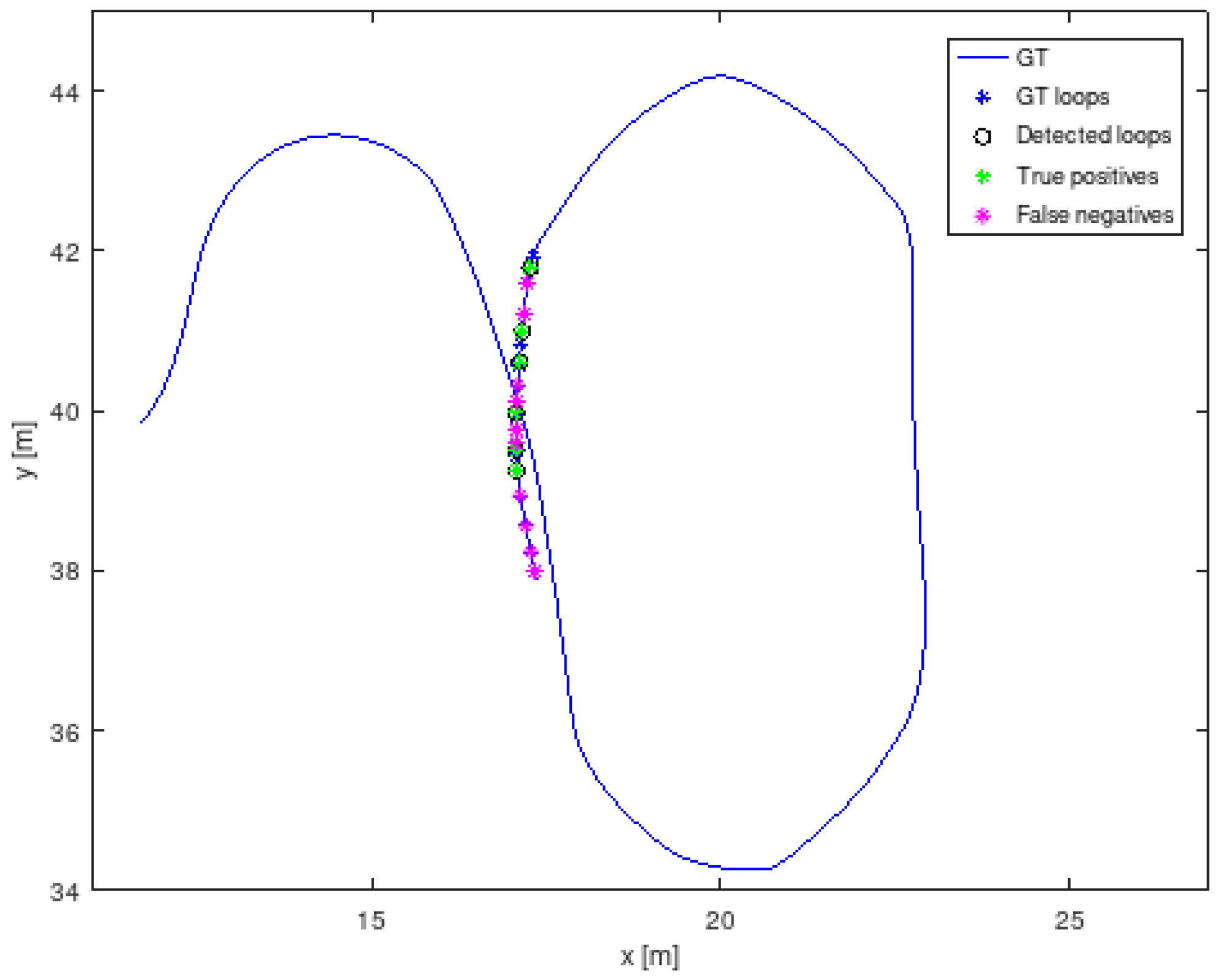
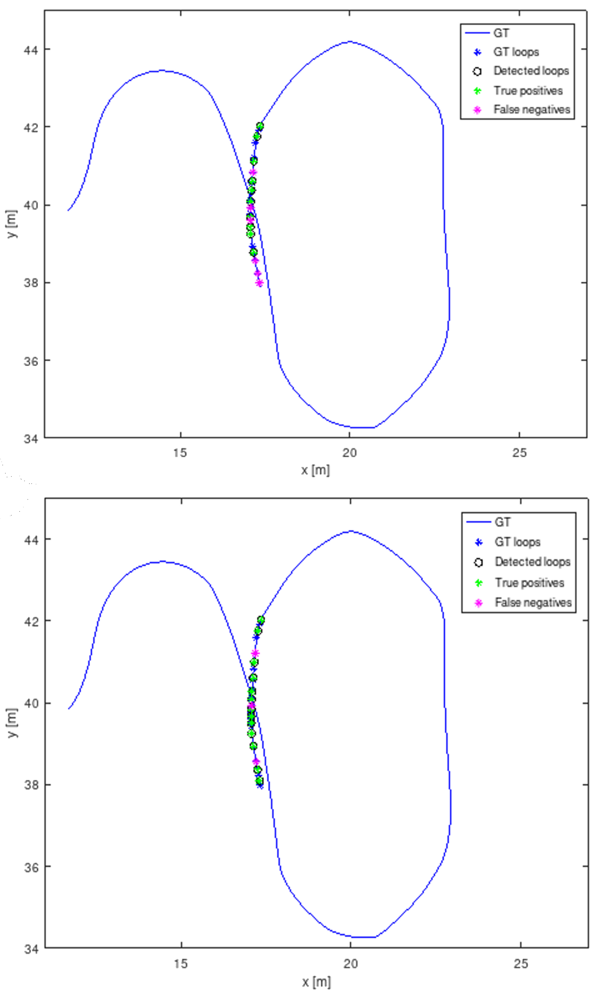
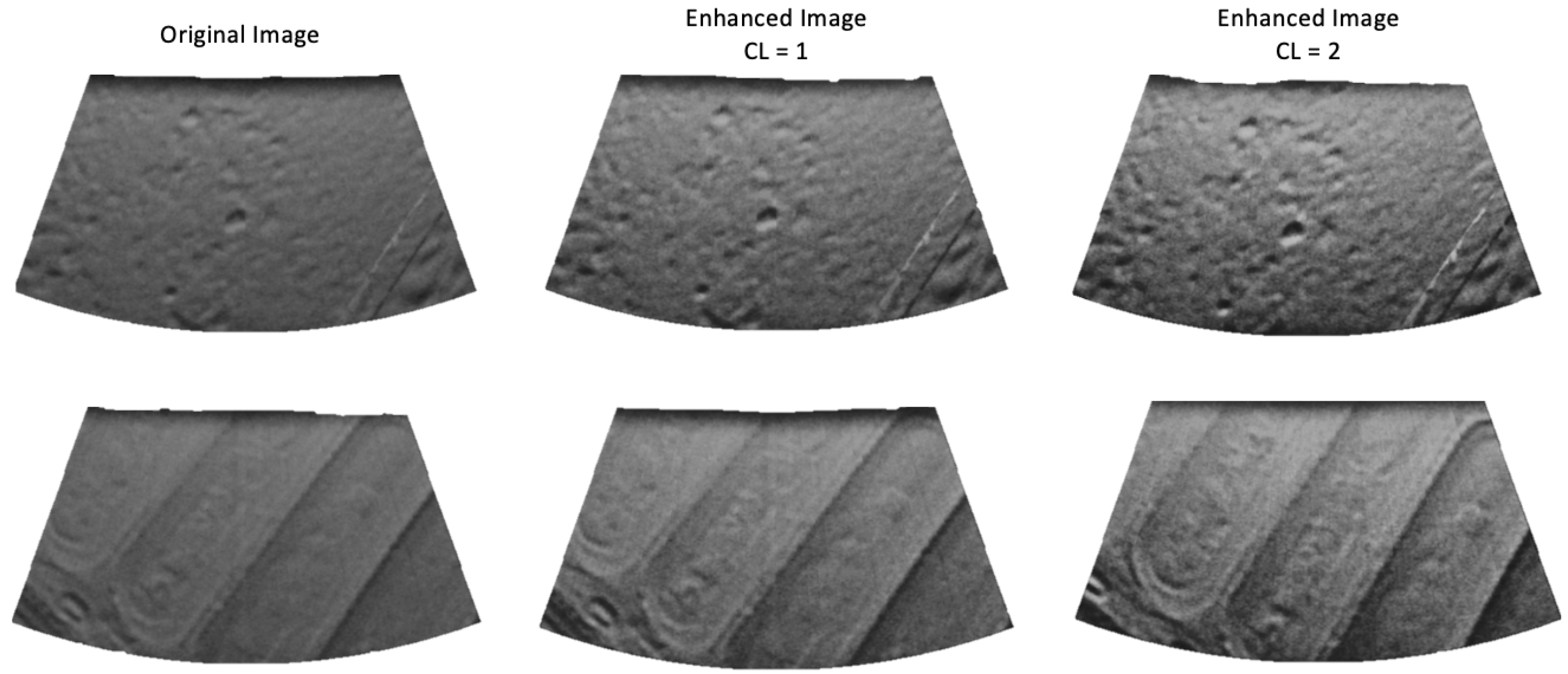
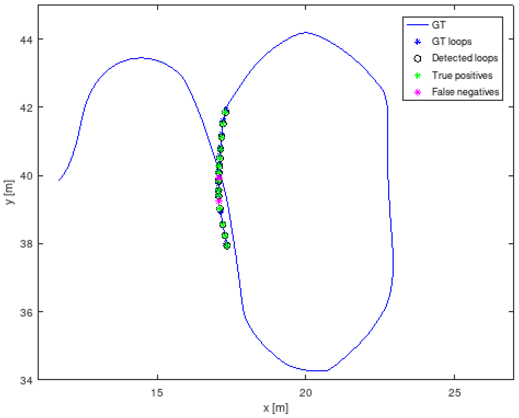
This paper presents a purely acoustic method for place recognition that can overcome the inherent limitations of perception in harbour scenarios. Poor visibility can complicate the behaviour of navigation and mapping tasks performed by cameras. Therefore, forward-looking sonars are a promising solution to extract information about the environment in such conditions as they do not suffer from these haze effects. These sensors suffer from distortion and occlusion effects. Their inherent characteristics include low signal-to-noise ratio and resolution, which is also inhomogeneous, and weak feature textures, so conventional feature-based techniques are not yet used for acoustic imaging. However, sonar performance has greatly improved and the resolution of these images is steadily increasing, allowing FLS to provide comprehensive underwater acoustic images. The proposed method aims to apply what is known about visual data to acoustic data to assess whether it is effective in detecting loops at close range, and then utilise its potential in conditions where cameras can no longer provide such distinguishable information. Given the lack of online data for these applications, and to allow for variations in environment parameters and sensor configurations, the Stonefish was utilised. Harbour facilities were simulated with this method to mimic the inspection work usually carried out in these areas. The autonomous vehicle performed a simple trajectory with a loop closure while the robot moved around the concrete wall. The vehicle navigated between waypoints close to structures, i.e., about 2–3 m, with the FLS facing the ground. Therefore, the sensor was adjusted accordingly and an odometry sensor was also used to obtain ground truth data. Considering the features that may affect the image quality and thus the subsequent imaging processes such as feature extraction and matching, the effectiveness of the acoustic features was evaluated. To this end, a functional analysis was performed to understand the performance of the ORB features. Thus, the ORB was quantified by measuring the number of detected keypoints on each image and the number of corresponding keypoints based on Hamming distance, since the features are binary. Finally, the effective matches between consecutive images, i.e., the inliers, were measured based on RANSAC, where the more similar the images are, the higher the value. The behaviour of the visual images was also measured based on these metrics to understand the performance of the acoustic images. In general, under normal viewing conditions, the sonar data provide fewer features than the camera images. However, when the visual images are made more difficult, the performance of the FLS remains the same, while that of the optical sensor decreases, reaching 18 points, of which the FLS can recognise 41 in low-light conditions. In order to understand the impact of turbidity values on the visual images, this parameter was increased in the simulator, but not for severe values. The matching performance between consecutive images decreases sharply; the algorithm detects about 80 fewer inliers compared to normal visibility conditions, suggesting that optical-based methods are sensitive to such severe conditions and may fail in detecting loop closures. Considering this degradation of visual data performance in poor visibility conditions, which is dangerous in a navigation context, it was investigated whether FLS can help find similar images in such conditions to recognise that the vehicle is already in a certain area and thus enable a correct estimation of the vehicle position. To measure the behaviour of the presented acoustic approach, the metrics precision and recall were calculated. Based on the standard thresholds commonly used for optical images, i.e., considering $\alpha$ = 0.3 and minFPnts = 12, the algorithm does not falsely recognise situations where a loop closes, i.e., FP = 0 and 100% precision. However, the strength of the algorithm is low as it tends to lose loops along the trajectory. It only recognises six situations where loops close, achieving 37.5% of recall. This performance is unsuitable for navigation purposes as there are no adjustments to the trajectory. Therefore, the requirements for the similarity threshold and the minimum number of inliers were analysed. The lower the similarity threshold, the more situations in which the loop closes are detected by the method. Nevertheless, the performance improvements are not very significant. If the minimum value of matches between the images is lowered so that they are considered to be the same location, it is obvious that the algorithm can recognise more loop closures. However, a balance must be found to achieve a quality trade-off. With 10 inliers as the minimum threshold and $\alpha$ = 0.3, the algorithm recognises 10 loops and achieves 62.5% recall and 100% precision. However, the experiments show that the features are not robust and therefore the matches are not distinguishable to benefit from the benevolence of the requirements. Therefore, the effect of an enrichment technique was evaluated to understand whether enrichment provides a better description of the images for acoustic image-based address place recognition. The CLAHE method was used as it was found to be the better choice for extracting additional information from low-contrast images. To improve the contrast and highlight the image edges, it depends on the parameterisation of two parameters: NT, which divides the images into equal square regions, and CL, which controls the noise enhancement. If we look at the resulting images, we can see that the contrast has been effectively increased and the details improved, so that more key points can be recognised compared to the original images. To understand whether there are any noisy pixels and whether these features are robust enough to increase the number of correct matches, we tested the behaviour of place detection for CL = 1 and CL = 2 as well as NT = [2, 3] and NT = [4, 6]. Initially, one would expect the recall to increase with contrast, but this only happens at the expense of reducing the geometric test requirements, i.e., by resorting to 10 inliers. Furthermore, the algorithm achieves the same maximum recall in two cases, but again with a lower value of inliers at CL = 2. Thus, it can be seen that more keypoints do not necessarily mean distinguishable points. Next, the number of image tiles was also increased, i.e., for NT = [4, 6], to find out whether the creation of more detailed histograms has an influence on the image description and consequently improves the similarity detection behaviour of the algorithm. In this case, increasing CL only increases recall at the expense of reducing the minimum matches for two images to be similar in content. Moreover, in this case with CL = 1, the algorithm achieves the same performance as in the previous case, but taking into account 10 inliers. It can therefore be assumed that an increase in the number of subdivisions is not accompanied by a better description of the images. In all cases, a precision of 100% is achieved, which means that there are no misidentified loops, i.e., CLAHE increases the image details and maintains the distinctiveness of the features for the similarity threshold used. Thus, the experiments show that increasing both parameters does not lead to a better description of the scene. Under the same assumptions, the most balanced result was obtained with CL = 1 and NT = [2, 3]. Under these conditions, the proposed FLS-based approach only fails for two loop closures and achieves a recall of 87.5%, which corresponds to an increase of 50% compared to the original result. The experiments show that the typically weak texture of FLS images contributes to the algorithm achieving a precision of 100% in all cases. Even if you lower the similarity threshold, this behaviour is not affected. This performance is crucial in a navigation context where the goal is to maximise recall at 100% precision, as this way no wrong trajectory adjustments are made which can lead to a wrong pose estimation of the vehicle. On the other hand, this fact complicates the strength of the algorithm not to miss any loops during the trajectory, as a minimum of consistent matches between images is required. Therefore, the enhancement technique improves the behaviour of the algorithm, i.e., it increases the image contrast and details (without noisy pixels) and more effective features are detected. For this reason, there are no features that could confuse the algorithm and thus affect its robustness in correctly recognising a place. Since the images of the FLS are based on emitted and returned sounds, the behaviour of the FLS is the same regardless of the environment conditions. This indicates that the FLS supports loop detection in poor visibility when the camera no longer provides detailed information.

In short, the place detection mechanism is therefore essential to avoid cumulative positioning errors. Indeed, visual loop detection is widely used because cameras provide a large amount of information and are very robust at short distances. However, these sensors are sensitive to visibility conditions. Considering that acoustic sensors do not suffer from these turbidity effects, this work has opened new horizons and showed that they can be of great help for underwater vehicles to perceive the environment in low-visibility conditions and thus not jeopardise the task of navigation near structures. Therefore, an adaptive navigation method can be interesting to improve the ability of vehicles to navigate in real underwater scenarios. The idea can be that the vehicle activates the most appropriate sensor depending on the conditions encountered during the mission. For example, when inspecting structures, i.e., close-range missions, the vehicle can navigate based on the camera to perceive the environment and activate the forward-looking sonar when visibility is insufficient (turbidity, darkness or brightness). If the area is poorly textured, a laser, i.e., a structured light system, can also be switched on.

New and more complex inspection trajectories are planned for the future to test the behaviour of FLS when the scene is viewed from different angles. Furthermore, other strategies to measure the similarity between images and data representation, i.e., indexing methods, will be evaluated to compare them with the performance of the proposed approach. Furthermore, it is planned to determine the conditions and limits of interaction between the two sensors—camera and FLS—in order to develop a hybrid solution for place recognition in underwater scenes. An evaluation of this approach in real harbour facilities is also planned.