
Navigating Energy Efficiency: A Multifaceted Interpretability of Fuel Oil Consumption Prediction in Cargo Container Vessel Considering the Operational and Environmental Factors


Abstract
:1. Introduction
1.1. Background of Study
1.2. Aim of the Study
- Build an accurate predictive model using a regression-based model to forecast vessel fuel oil consumption (FOC) based on operational and environmental variables. The model performance will be evaluated using metrics like R-squared, RMSE, and MAE.
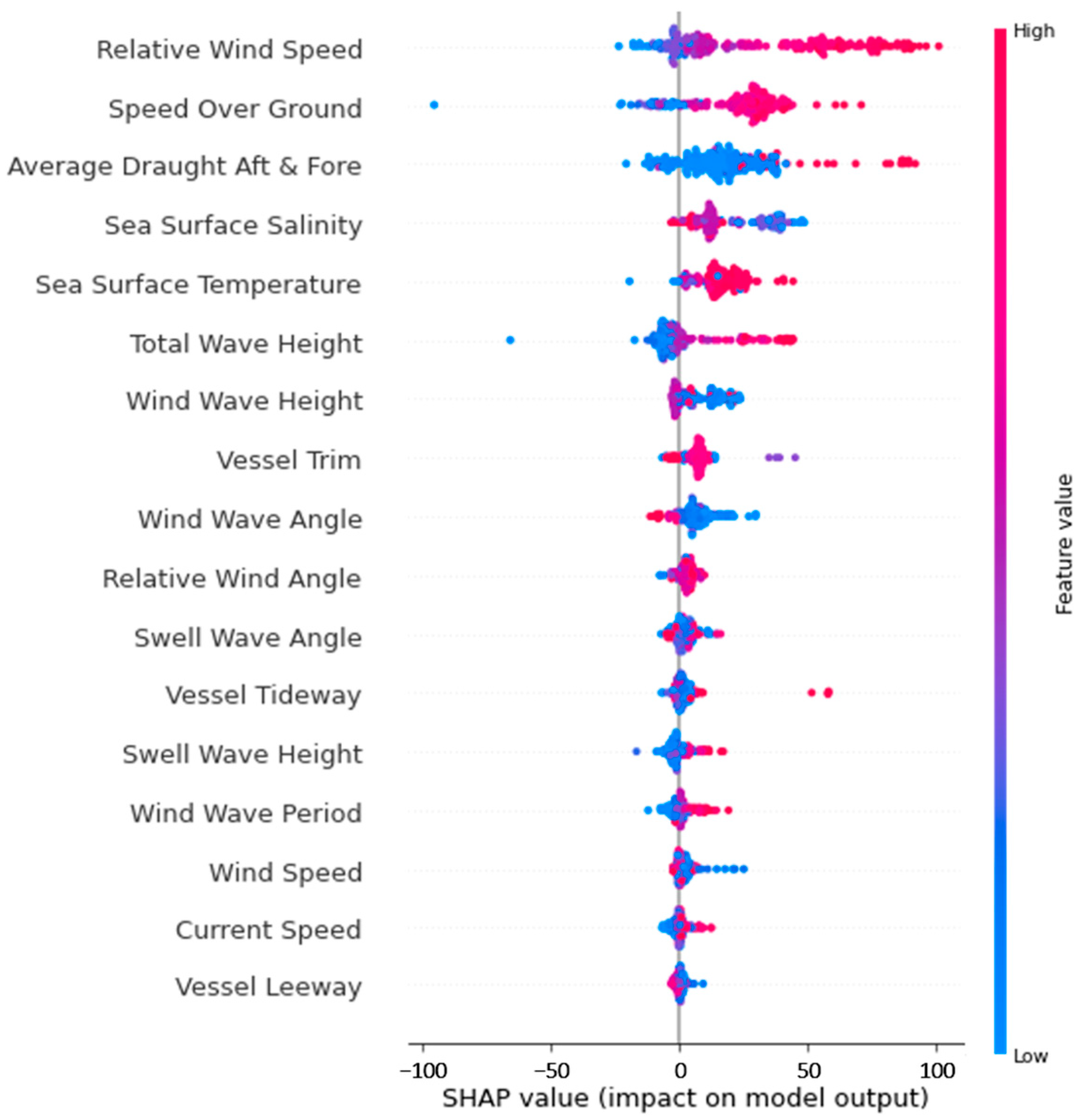
- Interpret the key drivers of the model’s predictions using SHAP values to understand how factors influence expected FOC under different conditions. This can reveal the most important controllable and uncontrollable factors overall.
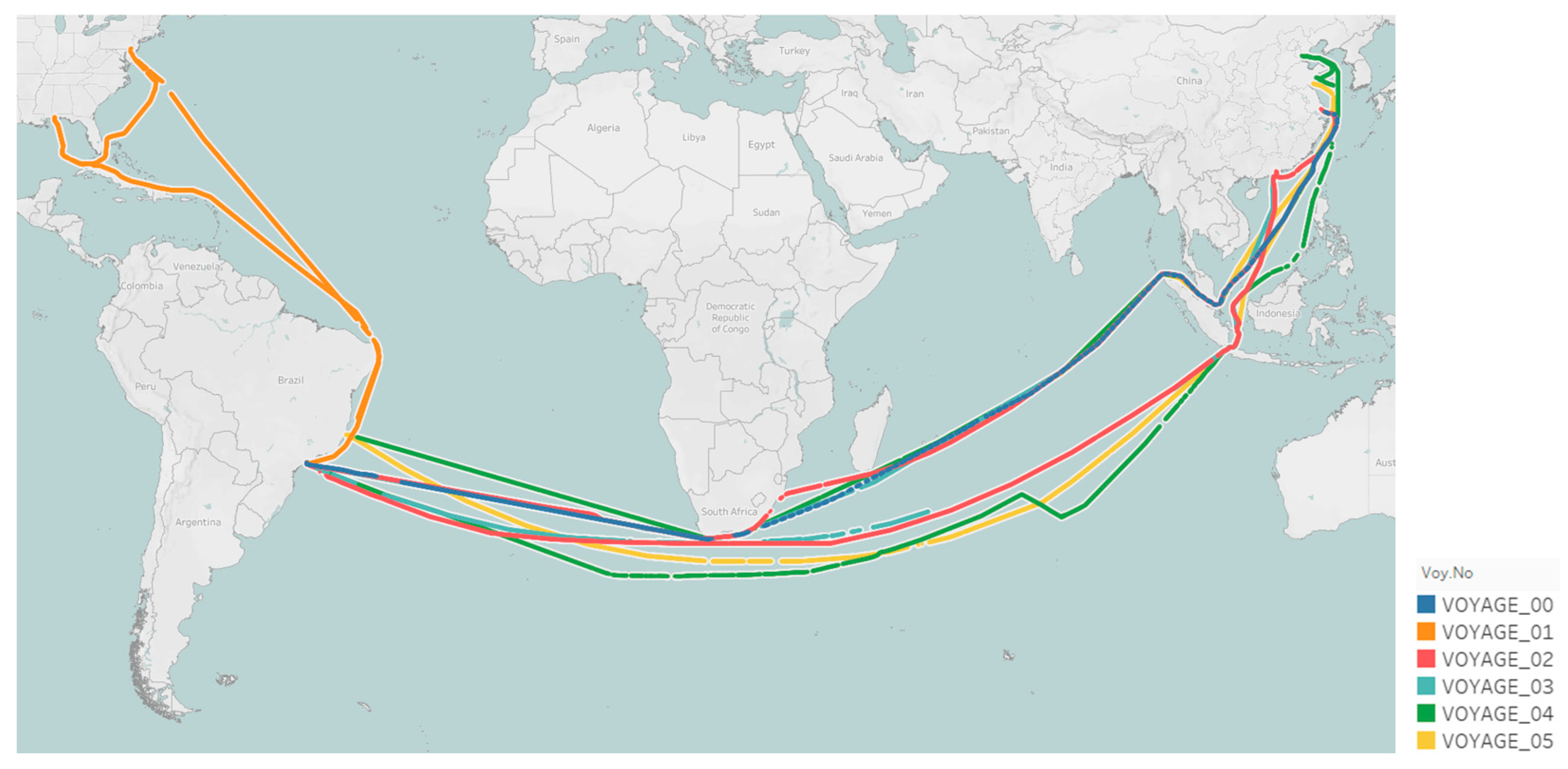
- Analyze regions or vessel routes where the model forecasts extremely high FOC and explore if differences exist in the factors’ relative importance rankings—identifying region-specific consumption drivers to guide context-specific optimizations.
- Provide recommendations for optimizing vessel operations, routing, and design based on the model interpretation. This includes suggestions for controlling influential operational parameters and mitigating uncontrollable factors where possible.
- Present findings in a way that helps stakeholders in the maritime industry enhance decision-making regarding energy efficiency improvements through better comprehension of complex FOC determinants.
2. Literature Review
2.1. Existing Research
2.2. Research Gaps and Contributions
3. Data and Methodologies
3.1. Data Overview
3.1.1. Data Acquisition
3.1.2. Feature Selection
3.2. Data Preprocessing
3.2.1. Data Filtering
3.2.2. Feature Transformation
3.3. Methodologies
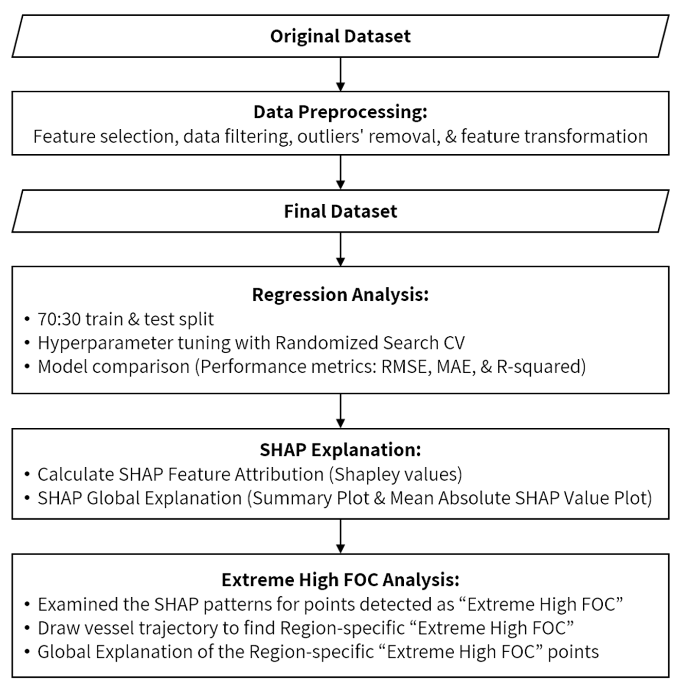
- Data Preprocessing: The dataset underwent data cleaning including filtering outliers and implausible values. Key features were also engineered from raw measurements, as explained in Section 3.2. This prepared the data for modeling.
- Regression Analysis: The preprocessed data was split 70% for model training and 30% for testing. This commonly used split ratio provides sufficient data for fitting while reserving an independent portion for unbiased evaluation. Three regressor models were tuned and trained. Its performance was evaluated on the test set using metrics like R-squared, RMSE, MAE, and MAPE to quantify predictive accuracy. The best regressor was developed to predict FOC using the training set.
- IQR Analysis: The interquartile range was determined to identify outlier FOC values above the third quartile, indicating potentially extreme consumption. Focusing interpretation on these points aimed to uncover dynamics in atypical usage scenarios.
- SHAP Explanation: Model explanations are crucial to support complex decision-making. SHAP values were computed to highlight the relative impact of each input on FOC predictions, increasing the comprehensibility of consumption determinants.
- Extreme High FOC Analysis: Further analysis specifically examined the SHAP patterns for points detected as extremely high FOC. Region-specific analyses then explored whether certain areas exhibited divergent input importance trends compared to overall patterns.
3.3.1. Fuel Oil Consumption Prediction
3.3.2. Extreme High Fuel Oil Consumption Detection
3.3.3. SHAP Model Explanation
4. Results and Discussion
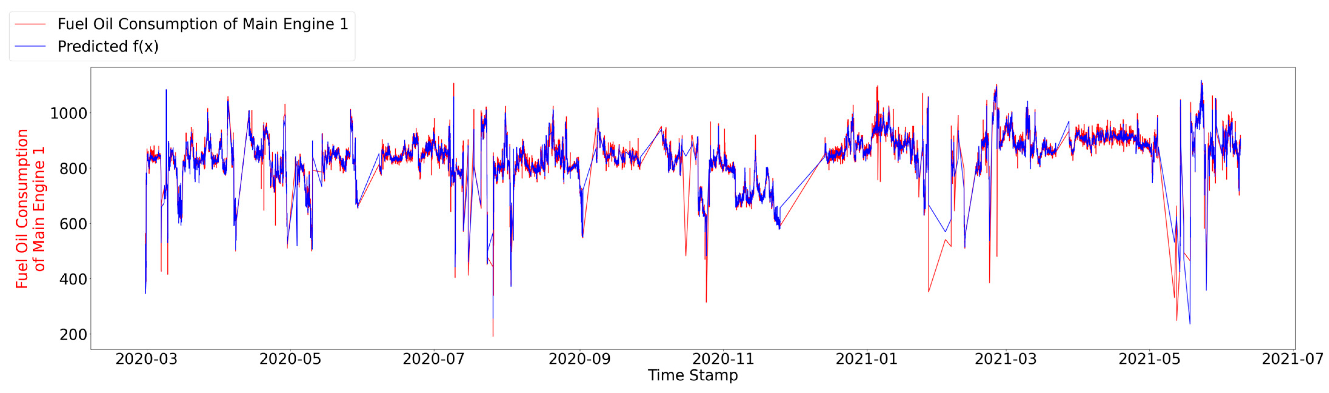
4.1. Fuel Oil Consumption Prediction
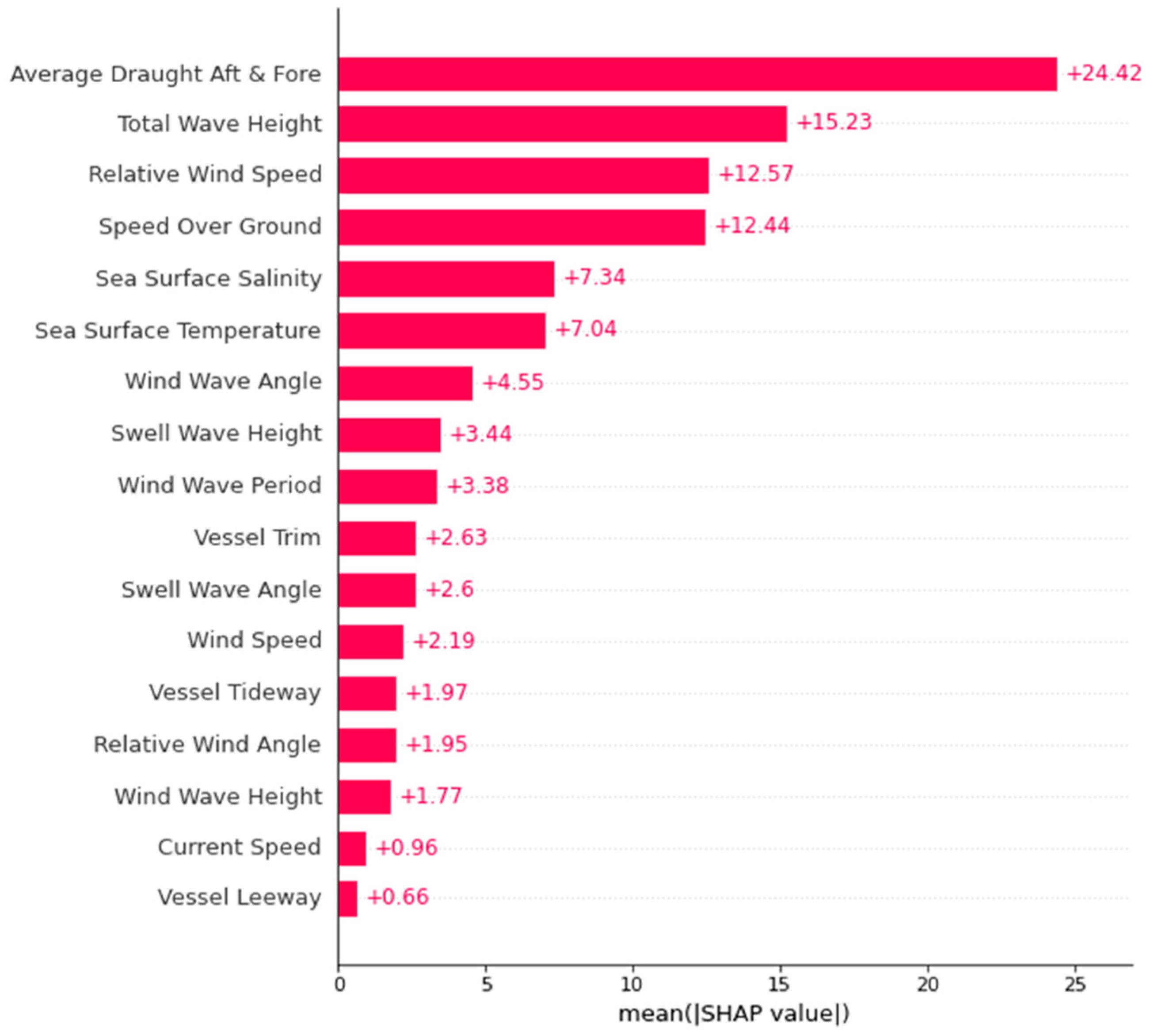
4.2. SHAP Global Explanation
4.2.1. Global Explanation of Overall Data
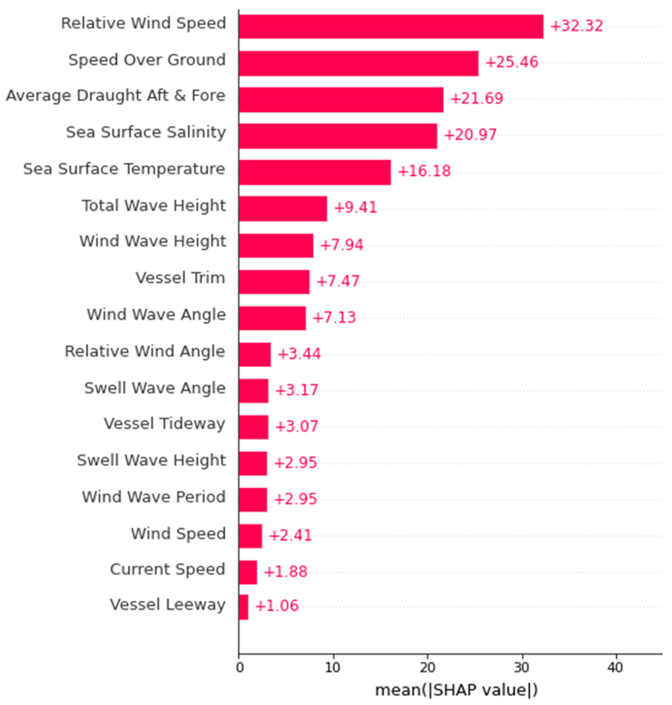
4.2.2. Global Explanation of Extremely High FOC
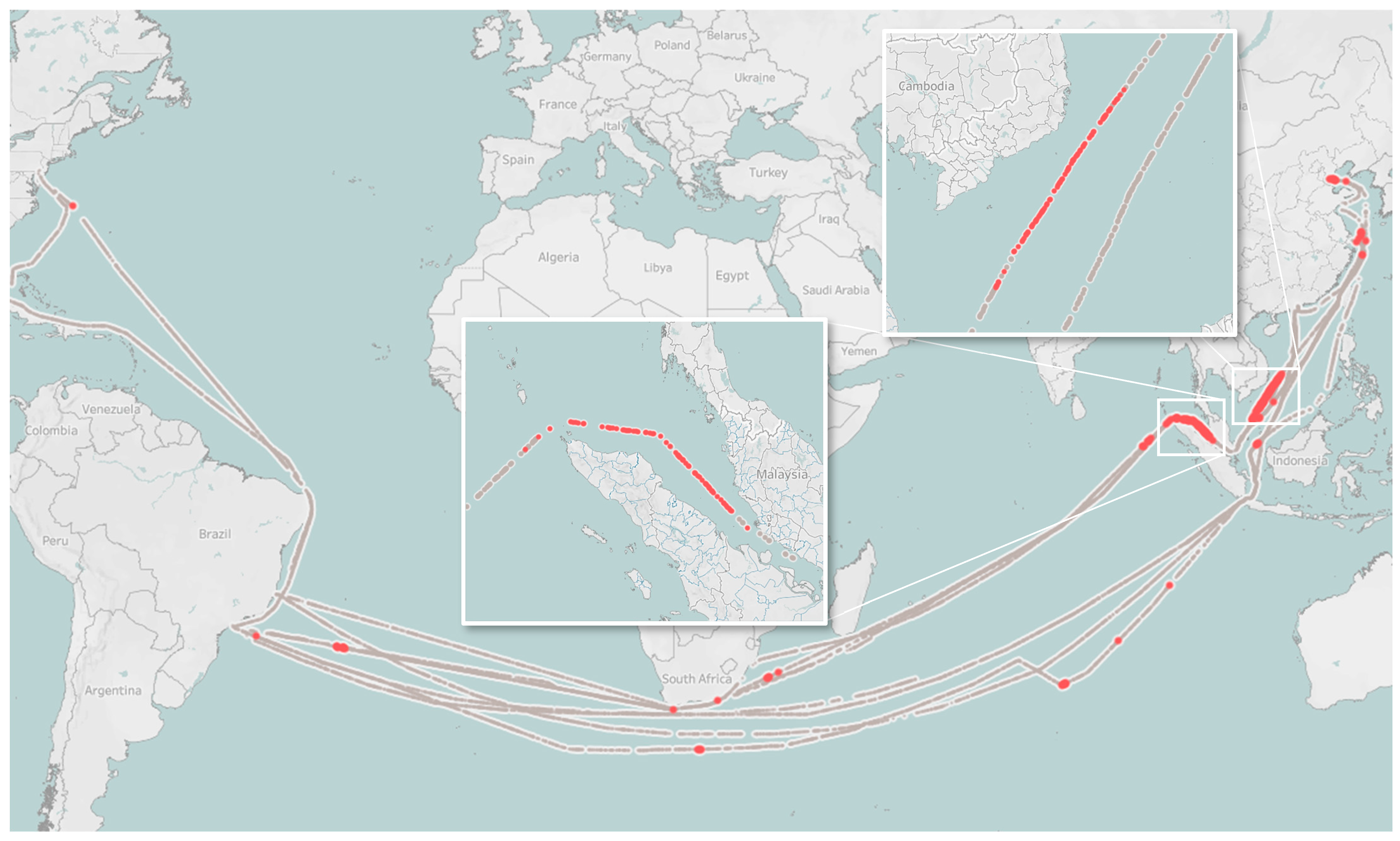
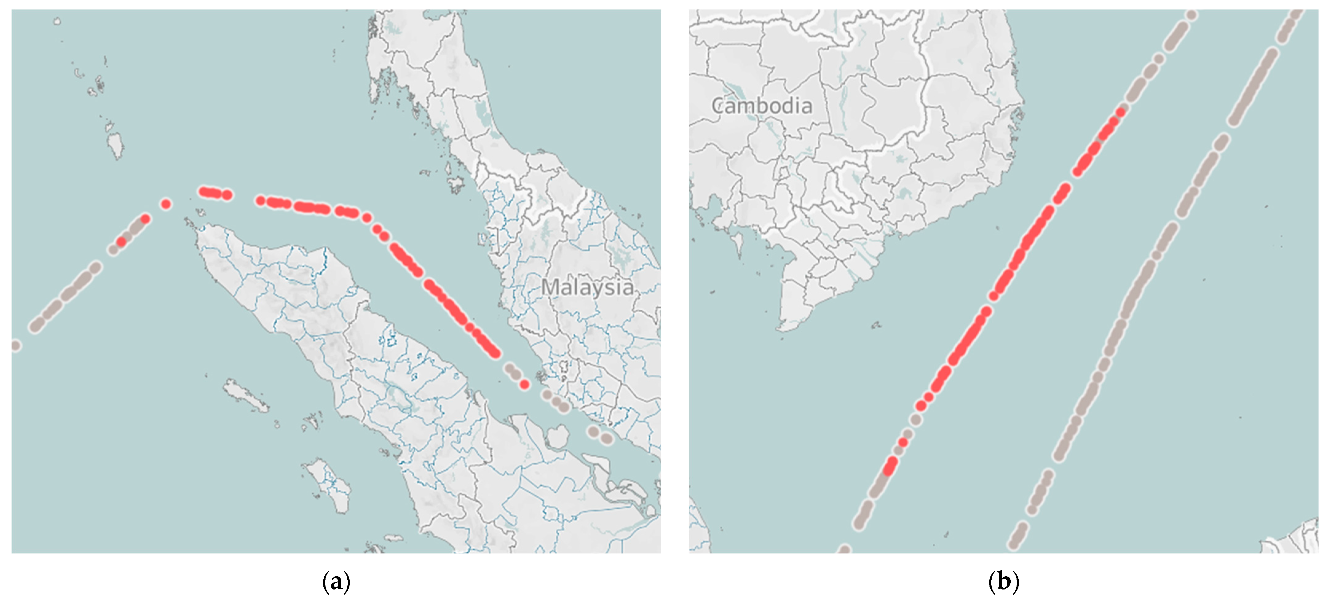
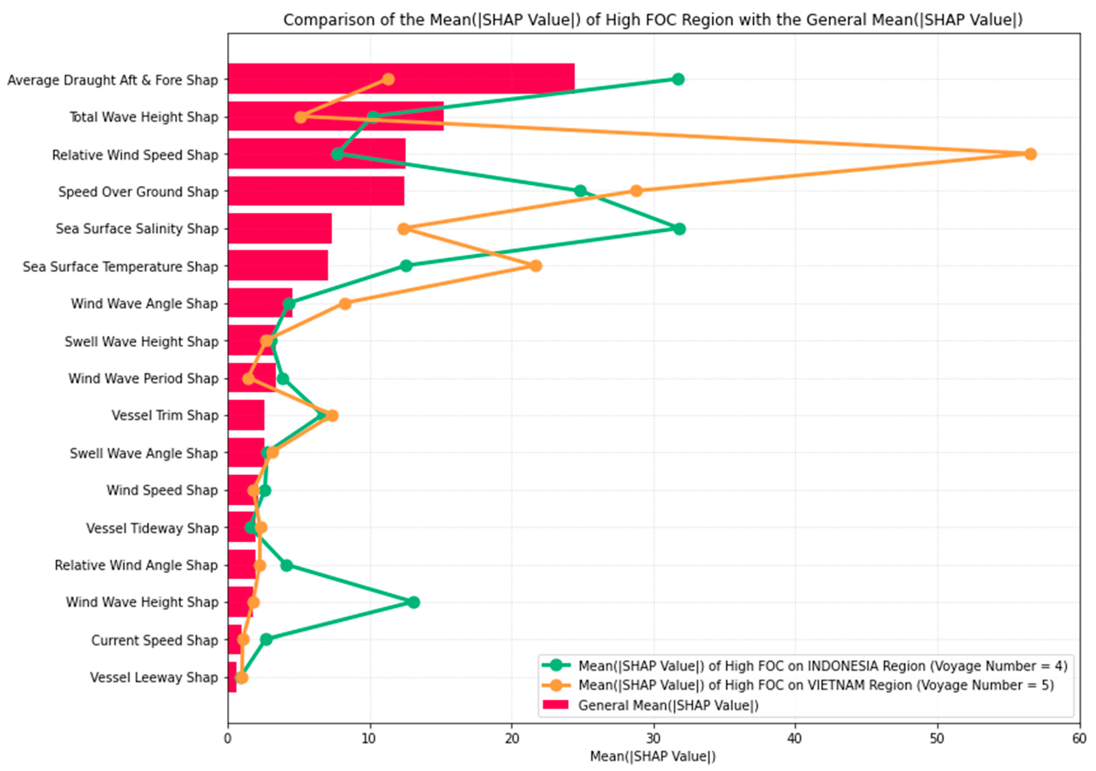
4.2.3. Region-Specific Extreme FOC Explanation
4.3. Discussion
4.3.1. Prediction Model Development
4.3.2. SHAP Global Explanation
- Fouling Influence: Higher sea surface temperatures and specific salinity levels can create more favourable conditions for the growth and distribution of fouling organisms. The accumulation of fouling on a ship’s hull and propeller increases hydrodynamic drag and leads to higher resistance, necessitating increased fuel consumption for the ship to maintain its operational efficiency. These conditions can also affect the kinematic viscosity of seawater, further elevating resistance.
- Kinematic Viscosity: The alteration of seawater properties by temperature and salinity influences kinematic viscosity, impacting the flow of water around the ship’s hull. Higher kinematic viscosity can result in elevated resistance, requiring more energy to propel the vessel. The pronounced effect of sea surface salinity and temperature on this viscosity may explain their high-ranking impact on fuel consumption.
4.3.3. Region-Specific Extreme FOC Explanation
5. Conclusions
Author Contributions
Funding
Institutional Review Board Statement
Informed Consent Statement
Data Availability Statement
Conflicts of Interest
References
- UNCTAD. Trade and Environment Review 2023: Building A Sustainable and Resilient Ocean Economy Beyond 2030; United Nations Conference on Trade and Development (UNCTAD): Geneva, Switzerland, 2023; Available online: https://unctad.org/system/files/official-document/ditcted2023d1_en.pdf (accessed on 15 May 2023).
- DNV AS. Energy Transition Outlook 2022: A Global and Regional Forecast to 2050; DNV: Oslo, Norway, 2022. [Google Scholar]
- IRENA. A Pathway to Decarbonise the Shipping Sector by 2050; International Renewable Energy Agency (IRENA): Abu Dhabi, United Arab Emirates, 2021; Available online: https://www.irena.org/-/media/Files/IRENA/Agency/Publication/2021/Oct/IRENA_Decarbonising_Shipping_2021.pdf (accessed on 15 May 2023).
- DNV GL AS. Energy Transition Outlook 2020: A Global and Regional Forecast to 2050; DNV: Oslo, Norway, 2020. [Google Scholar]
- Seddiek, I.S.; Ammar, N.R. Harnessing Wind Energy on Merchant Ships: Case Study Flettner Rotors Onboard Bulk Carriers. Environ. Sci. Pollut. Res. 2021, 28, 32695–32707. [Google Scholar] [CrossRef] [PubMed]
- IBarreiro, J.; Zaragoza, S.; Diaz-Casas, V. Review of Ship Energy Efficiency. Ocean Eng. 2022, 257, 111594. [Google Scholar] [CrossRef]
- Bayraktar, M.; Cerit, G.A. An Assessment on the Efficient Use of Hybrid Propulsion System in Marine Vessels. World J. Environ. Res. 2020, 10, 61–74. [Google Scholar] [CrossRef]
- Mansoursamaei, M.; Moradi, M.; González-Ramírez, R.G.; Lalla-Ruiz, E. Machine Learning for Promoting Environmental Sustainability in Ports. J. Adv. Transp. 2023, 2023, 2144733. [Google Scholar] [CrossRef]
- Akyuz, E.; Cicek, K.; Celik, M. A Comparative Research of Machine Learning Impact to Future of Maritime Transportation. Procedia Comput. Sci. 2019, 158, 275–280. [Google Scholar] [CrossRef]
- Li, H.; Yang, Z. Incorporation of AIS Data-Based Machine Learning into Unsupervised Route Planning for Maritime Autonomous Surfave Ships. Transp. Res. Part E Logist. Transp. Rev. 2023, 176, 103171. [Google Scholar] [CrossRef]
- Zis, T.P.V.; Psaraftis, H.N.; Ding, L. Ship Weather Routing: A Taxonomy and Survey. Ocean Eng. 2020, 213, 107697. [Google Scholar] [CrossRef]
- Li, X.; Sun, B.; Jin, J.; Ding, J. Speed Optimization of Container Ship Considering Route Segmentation and Weather Data Loading: Turning Point-Time Segmentation Method. J. Mar. Sci. Eng 2022, 10, 1835. [Google Scholar] [CrossRef]
- Du, Y.; Meng, Q.; Wang, S.; Kuang, H. Two-Phase Optimal Solutions for Ship Speed and Trim Optimization over a Voyage Using Voyage Report Data. Transp. Res. Part B Methodol. 2019, 122, 88–114. [Google Scholar] [CrossRef]
- Ksciuk, J.; Kuhlemann, S.; Tierney, K.; Koberstein, A. Uncertainty in Maritime Ship Routing and Scheduling: A Literature Review. Eur. J. Oper. Res. 2023, 308, 499–524. [Google Scholar] [CrossRef]
- Makridis, G.; Kyriazis, D.; Plitsos, S. Predictive Maintenance Leveraging Machine Learning for Time-Series Forecasting in the Maritime Industry. In Proceedings of the 2020 IEEE 23rd International Conference on Intelligent Transportation Systems (ITSC), Rhodes, Greece, 20–23 September 2020. [Google Scholar] [CrossRef]
- Petry, L.M.; Soares, A.; Bogorny, V.; Brandoli, B.; Matwin, S. Challenges in Vessel Behavior and Anomaly Detection: From Classical Machine Learning to Deep Learning. In Advances in Artificial Intelligence. Canadian AI 2020; Lecture Notes in Computer Science; Goutte, C., Zhu, X., Eds.; Springer: Cham, Switzerland, 2020; Volume 12109. [Google Scholar] [CrossRef]
- Laurie, A.; Anderlini, E.; Dietz, J.; Thomas, G. Machine Learning for Shaft Power Prediction and Analysis of Fouling Related Performance Deterioration. Ocean Eng. 2021, 234, 108886. [Google Scholar] [CrossRef]
- Kretschmann, L. Leading Indicators and Maritime Safety: Predicting Future Risk with a Machine Learning Approach. J. Shipp. Trade 2020, 5, 19. [Google Scholar] [CrossRef]
- Park, H.J.; Lee, M.S.; Park, D.I.; Han, S.W. Time-Aware and Feature Similarity Self-Attention in Vessel Fuel Consumption Prediction. Appl. Sci. 2021, 11, 11514. [Google Scholar] [CrossRef]
- Soleymani, A.; Sharifi, S.M.H.; Edalat, P.; Sharifi, S.M.M.; Zadeh, S.K. Linear Modelling of Marine Vessels Fuel Consumption for Ration of Subsidized Fuel. Int. J. Marit. Technol. 2018, 10, 7–13. [Google Scholar] [CrossRef]
- Uyanik, T.; Arslanoglu, Y.; Kalenderli, O. Ship Fuel Consumption Prediction with Machine Learning. In Proceedings of the 4th International Mediterranean Science and Engineering Congress, Antalya, Turkey, 25–27 April 2019; Available online: https://www.researchgate.net/profile/Tayfun-Uyanik/publication/332717845_Ship_Fuel_Consumption_Prediction_with_Machine_Learning/links/5ecd0608299bf12a632d479f/Ship-Fuel-Consumption-Prediction-with-Machine-Learning.pdf (accessed on 15 May 2023).
- Ren, F.; Wang, S.; Liu, Y.; Han, Y. Container Ship Carbon and Fuel Estimation in Voyages Utilizing Meteorological Data with Data Fusion and Machine Learning Techniques. Math. Program Eng. 2022, 2022, 4773395. [Google Scholar] [CrossRef]
- Uyanık, T.; Karatuğ, Ç.; Arslanoğlu, Y. Machine Learning Approach to Ship Fuel Consumption: A Case of Container Vessel. Transp. Res. Part D Transp. Environ. 2020, 84, 102389. [Google Scholar] [CrossRef]
- Wang, S.; Ji, B.; Zhao, J.; Liu, W.; Xu, T. Predicting Ship Fuel Consumption Based on LASSO Regression. Transp. Res. Part D Transp. Environ. 2018, 65, 817–824. [Google Scholar] [CrossRef]
- Peng, Y.; Liu, H.; Li, X.; Huang, J.; Wang, W. Machine Learning Method for Energy Consumption Prediction Of Ships in Port Considering Green Ports. J. Clean. Prod. 2020, 264, 121564. [Google Scholar] [CrossRef]
- Zhao, S.; Yin, Q.; Chen, X.; Zhao, F.; Zhao, K.; Zheng, J. Influence of Different Machine Learning Algorithms on Prediction Model of Fuel Consumption of Inland Ships. In Proceedings of the 2021 6th International Conference on Transportation Information and Safety (ICTIS), Wuhan, China, 22–24 October 2021. [Google Scholar] [CrossRef]
- Yan, R.; Wang, S.; Yuquan, D. Development of a Two-Stage Ship Fuel Consumption Prediction and Reduction Model for a Dry Bulk Ship. Transp. Res. Part E Logist. Transp. Rev. 2020, 138, 101930. [Google Scholar] [CrossRef]
- Yuan, J.; Nian, V. Ship Energy Consumption Prediction with Gaussian Process Metamodel. Energy Procedia 2018, 153, 655–660. [Google Scholar] [CrossRef]
- Moreira, L.; Vettor, R.; Soares, C.G. Neural Network Approach for Predicting Ship Speed and Fuel Consumption. J. Mar. Sci. Eng. 2021, 9, 119. [Google Scholar] [CrossRef]
- Bui-Duy, L.; Vu-Thi-Minh, N. Utilization of a Deep Learning-Based Fuel Consumption Model in Choosing a Liner Shipping Route for Container Ships in Asia. Asian J. Shipp. Logist. 2021, 37, 1–11. [Google Scholar] [CrossRef]
- Hu, Z.; Jin, Y.; Hu, Q.; Sen, S.; Zhou, T.; Osman, M.T. Prediction of Fuel Consumption for Enroute Ship Based on Machine Learning. IEEE Access 2019, 7, 119497–119505. [Google Scholar] [CrossRef]
- Arrieta, A.B.; Díaz-Rodríguez, N.; Ser, J.D.; Bennetot, A.; Tabik, S.; Barbado, A.; Garcia, S.; Gil-Lopez, S.; Molina, D.; Benjamins, R.; et al. Explainable Artificial Intelligence (XAI): Concepts, Taxonomies, Opportunities and Challenges toward Responsible AI. Inf. Fusion 2020, 58, 82–115. [Google Scholar] [CrossRef]
- Tiwari, R. Explainable AI (XAI) and Its Applications in Building Trust and Understanding in AI Decision-Making. Int. J. Sci. Res. Eng. Manag. 2023, 7, 1. [Google Scholar] [CrossRef]
- Angelov, P.P.; Soares, E.A.; Jiang, R.; Arnold, N.I.; Atkinson, P.M. Explainable artificial intelligence: An analytical review. Wiley Interdiscip. Rev. Data Min. Knowl. Discov. 2021, 11, e1424. [Google Scholar] [CrossRef]
- Samek, W.; Wiegand, T.; Müller, K.-R. Explainable Artificial Intelligence: Understanding, Visualizing and Interpreting Deep Learning Models. arXiv 2017, arXiv:1708.08296. [Google Scholar]
- Sarp, S.; Kuzlu, M.; Wilson, E.; Cali, U.; Guler, O. A Highly Transparent and Explainable Artificial Intelligence Tool for Chronic Wound Classification: XAI-CWC. Preprints 2021, 1. [Google Scholar] [CrossRef]
- Kim, D.; Handayani, M.P.; Lee, S.; Lee, J. Feature Attribution Analysis to Quantify the Impact of Oceanographic and Maneuverability Factors on Vessel Shaft Power Using Explainable Tree-Based Model. Sensors 2023, 23, 1072. [Google Scholar] [CrossRef]
- Kim, D.; Antariksa, G.; Handayani, M.P.; Lee, S.; Lee, J. Explainable Anomaly Detection Framework for Maritime Main Engine Sensor Data. Sensors 2021, 21, 5200. [Google Scholar] [CrossRef]
- Chen, T.; Guestrin, C. XGBoost: A Scalable Tree Boosting System. In Proceedings of the 22nd ACM SIGKDD International Conference on Knowledge Discovery and Data Mining, San Fransisco, CA, USA, 13–17 August 2016; pp. 787–794. [Google Scholar] [CrossRef]
- Ribeiro, M.T.; Singh, S.; Guestrin, C. “Why Should I Trust You?”: Explaining the Predictions of Any Classifier. In Proceedings of the KDD ’16: Proceedings of the 22nd ACM SIGKDD International Conference on Knowledge Discovery and Data Mining, San Fransisco, CA, USA, 13–17 August 2016. [Google Scholar] [CrossRef]
- Ribeiro, M.T.; Singh, S.; Guestrin, C. Anchors: High-Precision Model-Agnostic Explanations. In Proceedings of the AAAI Conference of Artificial Intelligence, New Orleans, LA, USA, 2–7 February 2018. [Google Scholar] [CrossRef]
- Lundberg, S.M.; Lee, S.-I. A Unified Approach to Interpreting Model Predictions. In Proceedings of the Advances in Neural Information Processing Systems 30 (NIPS 2017), Long Beach, CA, USA, 4–9 December 2017; Available online: https://proceedings.neurips.cc/paper_files/paper/2017/file/8a20a8621978632d76c43dfd28b67767-Paper.pdf (accessed on 15 May 2023).
- Lundberg, S.M.; Erion, G.; Chen, H.; DeGrave, A.; Prutkin, J.M.; Nair, B.; Katz, R.; Himmelfarb, J.; Bansal, N.; Lee, S.-I. From Local Explanations to Global Understanding with Explainable AI for Trees. Nat. Mach. Intell. 2020, 2, 56–67. [Google Scholar] [CrossRef] [PubMed]
- Shapley, L.S. A Value for N-Person Games. In Contribution to the Theory of Games II; Princeton University Press: Princeton, NJ, USA, 1953; pp. 307–317. [Google Scholar]
- Hart, S. Shapley Value. In Game Theory; Palgrave Macmillan: London, UK, 1989; pp. 210–216. [Google Scholar]


| Citation | Model | Number of Predictors | XAI | |||
|---|---|---|---|---|---|---|
| Operational | Environmental | Engine | Vessel Characteristics | |||
| [20] | Linear Regression | 3 | 0 | 0 | 2 | ✗ |
| [21] | Multiple Linear Regression | 1 | 3 | 1 | 0 | ✗ |
| [22] | Ridge Regression | 5 | 4 | 0 | 0 | ✗ |
| [23] | Support Vector Regressor | 3 | 0 | 16 | 0 | ✗ |
| [24] | Lasso Regression | 8 | 7 | 0 | 3 | ✗ |
| [25] | K-Nearest Neighbor Regressor | 11 | 0 | 0 | 4 | ✗ |
| [26] | Extra Tree Regressor | 2 | 4 | 0 | 0 | ✗ |
| [27] | Random Forest Regressor | 2 | 9 | 0 | 0 | ✗ |
| [28] | Gaussian Process Metamodel | 3 | 4 | 0 | 0 | ✗ |
| [29] | Artificial Neural Network (ANN) | 1 | 3 | 1 | 0 | ✗ |
| [30] | Deep Learning | 2 | 2 | 0 | 1 | ✗ |
| This Research | XGBoost Regressor | 5 | 13 | 0 | 0 | ✓ |
| Register | Capacity | Size | |||
|---|---|---|---|---|---|
| Type | General Cargo | Gross Tonnage | 41,416 | Length (m) | 201 |
| Year Built | 2020 | Summer DWT (t) | 62,321 | Breadth (m) | 34 |
| Feature Name | Unit | Description |
|---|---|---|
| Main Engine 1 FOC | kg/h | Fuel oil consumption of main engine 1 |
| Speed Over Ground | knots | Vessel speed relative to the ground |
| Draught Fore | m | Distance between the waterline and the bottom of the vessel at the bow (front) end |
| Draught Aft | m | Distance between the waterline and the bottom of the vessel at the stern (back) end |
| Current Speed | m/s | Directional movement of seawater driven by gravity, wind, and water density |
| Wind Speed | m/s | Speed of the geographic or ground wind, assuming no tidal flow |
| Relative Wind Speed | m/s | Wind speed adjusted for the speed at which the vessel is traveling |
| Sea Surface Salinity | PSU | Salt concentration of the ocean water at the surface |
| Sea Surface Temperature | °C | Measure of heat in degrees at the top layer of the surrounding sea |
| Total Wave Height | m | Vertical distance between trough and crest including all wave components |
| Swell Wave Height | m | Height of the long-period waves not affected by local winds |
| Wind Wave Height | m | Height of gravity waves on the sea surface directly generated, sustained by wind |
| Wind Wave Period | s | Time interval between appearances of the same phase of a wind wave |
| Ship Heading | ° | Direction the vessel’s pointed end is facing, in degrees from north |
| Course Over Ground | ° | Direction of progress over the ground actually covered, regardless of heading |
| Rudder Angle | ° | Measured position of the vessel’s side-to-side steering mechanism |
| Current Direction | ° | Compass orientation of the flowing ocean water movement |
| Total Wave Direction | ° | Direction from which the combined wind and swell waves are coming from |
| Swell Wave Direction | ° | Direction the long regular ocean swells are originating from. |
| Wind Wave Direction | ° | Orientation the wind-generated waves are coming from. |
| Wind Direction | ° | Direction of the geographic or ground wind |
| Relative Wind Direction | ° | Measured angle of the wind in relation to the heading of the moving ship. |
| Feature Name | Unit | Description |
|---|---|---|
| Average Draught Aft and Fore | M | Average of draught fore and draught aft |
| Vessel Trim | M | Difference between draught fore and draught aft |
| Vessel Leeway | ° | Difference between ship heading and course over ground |
| Vessel Tideway | ° | Difference between ship heading and current direction |
| Wind Wave Angle | ° | Difference between ship heading and wind wave direction |
| Swell Wave Angle | ° | Difference between ship heading and swell wave direction |
| Relative Wind Angle | ° | Difference between ship heading and relative wind direction |
| Model | Parameters | ||
|---|---|---|---|
| Grid Parameters | Grid Values | Best Values | |
| XGBoost Regressor | n_estimators | : [100, 200, 300, 400] | {‘n_estimators’: 400, |
| reg_lambda | : [0, 0.1, 0.5, 1.0] | ‘reg_lambda’: 0.5, | |
| reg_alpha | : [0, 0.1, 0.5, 1.0] | ‘reg_alpha’: 0, | |
| min_child_weight | : [1, 2, 3, 4] | ‘min_child_weight’: 2, | |
| max_depth | : [3, 4, 5, 6] | ‘max_depth’: 6, | |
| learning_rate | : [0.01, 0.1, 0.2, 0.3] | ‘learning_rate’: 0.2, | |
| gamma | : [0, 0.1, 0.2, 0.3] | ‘gamma’: 0, | |
| colsample_bytree | : [0.6, 0.7, 0.8, 0.9, 1.0] | ‘colsample_bytree’: 0.6} | |
| CatBoost Regressor | n_estimators | : [100, 200, 300, 400] | {‘n_estimators’: 400, |
| max_depth | : [3, 4, 5, 6] | ‘max_depth’: 6, | |
| learning_rate | : [0.01, 0.1, 0.2, 0.3] | ‘learning_rate’: 0.3, | |
| l2_lear_reg | : [1, 3, 5, 7] | ‘l2_leaf_reg’: 5, | |
| bagging_temperature | : [0.0, 1.0, 2.0, 3.0] | ‘bagging_temperature’: 2.0} | |
| Gradient Boost Regressor | n_estimators | : [100, 200, 300, 400] | {‘n_estimators’: 400, |
| min_samples split | : [2, 3, 4, 5] | ‘min_samples_split’: 5, | |
| min_samples_leaf | : [1, 2, 3, 4] | ‘min_samples_leaf’: 1, | |
| max_features | : [‘auto’, ‘sqrt’, ‘log2’] | ‘max_features’: ‘log2’, | |
| max_depth | : [3, 4, 5, 6] | ‘max_depth’: 6, | |
| loss | : [‘ls’, ‘lad’, ‘huber’] | ‘loss’: ‘huber’, | |
| learning_rate | : [0.01, 0.1, 0.2, 0.3] | ‘learning_rate’: 0.3, | |
| alpha | : [0.0, 0.1, 0.5, 1.0] | ‘alpha’: 0.5} | |
| Model | R2 Score | RMSE | MAE | |||
|---|---|---|---|---|---|---|
| Train | Test | Train | Test | Train | Test | |
| XGBoost Regressor | 0.99 | 0.95 | 9.47 | 19.12 | 7.09 | 11.62 |
| CatBoost Regressor | 0.96 | 0.94 | 16.04 | 21.03 | 11.5 | 13.69 |
| Gradient Boost Regressor | 0.96 | 0.93 | 16.77 | 22.89 | 8.79 | 13.68 |
| Grid Parameter | Grid Values | Best Value |
|---|---|---|
| n_estimator | : [100, 200, 300, 400, 500] | 300 |
| max_depth | : [2, 3, 5, 7, 10] | 10 |
| learning_rate | : [0.005, 0.01, 0.1, 0.3] | 0.1 |
| reg_alpha | : [0.1, 1, 10, 50, 100, 200] | 1 |
| min_child_weight | : [1, 5, 10, 25, 50] | 10 |
| subsample | : [0.5, 0.75, 1.0] | 1.0 |
| colsample_bytree | : [0.8, 0.9, 1.0] | 0.8 |
| reg_lambda | : [0.1, 1, 10, 50, 100, 200] | 1 |
| R2 Score | RMSE | MAE | |||
|---|---|---|---|---|---|
| Train | Test | Train | Test | Train | Test |
| 0.99 | 0.95 | 8.73 | 18.54 | 6.14 | 10.78 |
| Feature Importance | Ranking | Mean (|SHAP Value|) | Mean (SHAP Value) | |||
|---|---|---|---|---|---|---|
| All Data | High | All Data | High | All Data | High | |
| Relative Wind Speed | #03 | #01 | 12.57 | 32.32 | −0.30 | 29.92 |
| Speed Over Ground | #04 | #02 | 12.44 | 25.46 | −1.84 | 22.04 |
| Average Draft (Aft and Fore) | #01 | #03 | 24.42 | 21.69 | 3.64 | 19.88 |
| Sea Surface Salinity | #05 | #04 | 7.34 | 20.97 | −0.60 | 20.90 |
| Sea Surface Temperature | #06 | #05 | 7.04 | 16.18 | −0.03 | 15.97 |
| Total Wave Height | #02 | #06 | 15.23 | 9.41 | 0.52 | 2.36 |
| Wind Wave Height | #15 | #07 | 1.77 | 7.94 | −0.33 | 7.13 |
| Vessel Trim | #10 | #08 | 2.63 | 7.47 | 0.51 | 6.94 |
| Wind Wave Angle | #07 | #09 | 4.55 | 7.13 | −0.28 | 5.96 |
| Relative Wind Angle | #14 | #10 | 1.95 | 3.44 | −0.65 | 2.99 |
| Swell Wave Angle | #11 | #11 | 2.60 | 3.17 | −0.60 | 2.17 |
| Vessel Tideway | #13 | #12 | 1.97 | 3.07 | 0.00 | 2.38 |
| Swell Wave Height | #08 | #13 | 3.44 | 2.95 | −0.54 | −0.19 |
| Wind Wave Period | #09 | #14 | 3.38 | 2.95 | 0.05 | 0.90 |
| Wind Speed | #12 | #15 | 2.19 | 2.41 | −0.03 | 2.14 |
| Current Speed | #16 | #16 | 0.96 | 1.88 | −0.04 | 0.08 |
| Vessel Leeway | #17 | #17 | 0.66 | 1.06 | −0.01 | 0.46 |
| Feature Importance | Feature Importance Ranking | Mean (|SHAP Value|) | Mean (SHAP Value) | |||||||||
|---|---|---|---|---|---|---|---|---|---|---|---|---|
| Overall | High | ID | VN | Overall | High | ID | VN | Overall | High | ID | VN | |
| Average Draught (Aft and Fore) | #01 | #03 | #02 | #05 | 24.42 | 21.69 | 31.73 | 11.30 | 3.64 | 19.88 | 30.68 | 9.80 |
| Total Wave Height | #02 | #06 | #06 | #08 | 15.23 | 9.41 | 10.24 | 5.10 | 0.52 | 2.36 | 0.49 | −0.23 |
| Relative Wind Speed | #03 | #01 | #07 | #01 | 12.57 | 32.32 | 7.74 | 56.53 | −0.30 | 29.92 | 3.42 | 56.46 |
| Speed Over Ground | #04 | #02 | #03 | #02 | 12.44 | 25.46 | 24.84 | 28.76 | −1.84 | 22.04 | 21.04 | 26.25 |
| Sea Surface Salinity | #05 | #04 | #01 | #04 | 7.34 | 20.97 | 31.84 | 12.39 | −0.60 | 20.90 | 31.84 | 12.39 |
| Sea Surface Temperature | #06 | #05 | #05 | #03 | 7.04 | 16.18 | 12.57 | 21.67 | −0.03 | 15.97 | 12.55 | 21.20 |
| Wind Wave Angle | #07 | #09 | #09 | #06 | 4.55 | 7.13 | 4.32 | 8.25 | −0.28 | 5.96 | 1.93 | 8.25 |
| Swell Wave Height | #08 | #13 | #12 | #10 | 3.44 | 2.95 | 3.06 | 2.74 | −0.54 | −0.19 | 0.56 | −1.54 |
| Wind Wave Period | #09 | #14 | #11 | #15 | 3.38 | 2.95 | 3.88 | 1.45 | 0.05 | 0.90 | 0.04 | 0.86 |
| Vessel Trim | #10 | #08 | #08 | #07 | 2.63 | 7.47 | 6.68 | 7.38 | 0.51 | 6.94 | 6.44 | 7.15 |
| Swell Wave Angle | #11 | #11 | #13 | #09 | 2.60 | 3.17 | 2.79 | 3.12 | −0.60 | 2.17 | 1.42 | 2.30 |
| Wind Speed | #12 | #15 | #15 | #13 | 2.19 | 2.41 | 2.64 | 1.83 | −0.03 | 2.14 | 2.41 | 1.45 |
| Vessel Tideway | #13 | #12 | #16 | #11 | 1.97 | 3.07 | 1.59 | 2.29 | 0.00 | 2.38 | 0.84 | 1.51 |
| Relative Wind Angle | #14 | #10 | #10 | #12 | 1.95 | 3.44 | 4.10 | 2.27 | −0.65 | 2.99 | 3.54 | 2.05 |
| Wind Wave Height | #15 | #07 | #04 | #14 | 1.77 | 7.94 | 13.08 | 1.80 | −0.33 | 7.13 | 13.07 | −0.02 |
| Current Speed | #16 | #16 | #14 | #16 | 0.96 | 1.88 | 2.68 | 1.06 | −0.04 | 0.08 | −0.89 | 0.78 |
| Vessel Leeway | #17 | #17 | #17 | #17 | 0.66 | 1.06 | 0.92 | 1.02 | −0.01 | 0.46 | 0.56 | 0.10 |
| General Condition | Extreme High FOC | Strait of Malacca | South China Sea | |
|---|---|---|---|---|
| Operational Optimization | Draft and speed control and monitoring Load adjustments | Speed adjustment given the wind conditions | Speed adjustment on the region that is suspected to have busy marine traffic | Speed reduction in response to high wind speed |
| Environmental Mitigation | Minimize voyage through high waves | Rerouting in high wind conditions | Monitor the distribution of salinity around the strait and a narrow shallow water area | Investigate the regional wind pattern and Munson effect |
Disclaimer/Publisher’s Note: The statements, opinions and data contained in all publications are solely those of the individual author(s) and contributor(s) and not of MDPI and/or the editor(s). MDPI and/or the editor(s) disclaim responsibility for any injury to people or property resulting from any ideas, methods, instructions or products referred to in the content. |
© 2023 by the authors. Licensee MDPI, Basel, Switzerland. This article is an open access article distributed under the terms and conditions of the Creative Commons Attribution (CC BY) license (https://creativecommons.org/licenses/by/4.0/).
Share and Cite
Handayani, M.P.; Kim, H.; Lee, S.; Lee, J. Navigating Energy Efficiency: A Multifaceted Interpretability of Fuel Oil Consumption Prediction in Cargo Container Vessel Considering the Operational and Environmental Factors. J. Mar. Sci. Eng. 2023, 11, 2165. https://doi.org/10.3390/jmse11112165
Handayani MP, Kim H, Lee S, Lee J. Navigating Energy Efficiency: A Multifaceted Interpretability of Fuel Oil Consumption Prediction in Cargo Container Vessel Considering the Operational and Environmental Factors. Journal of Marine Science and Engineering. 2023; 11(11):2165. https://doi.org/10.3390/jmse11112165
Chicago/Turabian StyleHandayani, Melia Putri, Hyunju Kim, Sangbong Lee, and Jihwan Lee. 2023. "Navigating Energy Efficiency: A Multifaceted Interpretability of Fuel Oil Consumption Prediction in Cargo Container Vessel Considering the Operational and Environmental Factors" Journal of Marine Science and Engineering 11, no. 11: 2165. https://doi.org/10.3390/jmse11112165
APA StyleHandayani, M. P., Kim, H., Lee, S., & Lee, J. (2023). Navigating Energy Efficiency: A Multifaceted Interpretability of Fuel Oil Consumption Prediction in Cargo Container Vessel Considering the Operational and Environmental Factors. Journal of Marine Science and Engineering, 11(11), 2165. https://doi.org/10.3390/jmse11112165