Empirical Shape-Based Estimation of Settling Microplastic Particles Drag Coefficient

Abstract

Microplastics (MP) are found in nature in various forms. The transport and settling process of MP particles in water streams is highly influenced by particle size and shape. In order to investigate the impact of particle shape, an experimental analysis of settling behavior of flat square particles and 3D cubic particles in flowing water was conducted. The analysis is based on tracking the settling trajectories of particles of various size and using this information for calculating the drag coefficient $c_d$ in relation to the Reynolds number Re in the range of 80 to 280 for cubes and 50 to 110 for flat particles. The results were correlated with two shape parameters, sphericity $\varphi$ and a newly proposed shape descriptor dimensionality $\delta$. The final output is a model for particle shape-based $c_d$ estimation, mainly serving as an illustration of the potential of the proposed methodology.

1. Introduction

A growing worry regarding the influence of microplastics (MP) on aquatic ecosystems necessitates ongoing research to enhance our comprehension of the process, scope, and magnitude of their impact [1,2,3,4]. Rivers carry land-based plastics to the ocean, leading to ecological harm in river ecosystems and posing risks to human health due to plastic pollution [5,6,7]. In order to effectively control and mitigate the transport of plastic waste in aquatic environments, gaining a deeper insight into their behavior within water flows is essential. The transport and settling velocity of solid particles in stagnant or flowing fluids is significantly influenced by drag force [8,9,10,11]. For spherical particles, there is a well-defined correlation between the drag coefficient $c_d$ and Reynolds number Re [12,13,14,15]. However, since the drag coefficient generally depends on both Re and particle shape, the behavior of specific non-spherical particles represents a widely researched topic in numerous scientific fields [16,17,18].

To assess the impact of particle shape, various dimensionless shape descriptors are used in the literature [19,20,21]. Khatmullina and Isachenko [22] proposed the use of Corey shape factor ($csf$), which is one of the most commonly used parameters for estimating the deviation of particle shape from a perfect sphere. Moreover, the authors suggested the need for further experiments with MP of different shapes. Kowalski et al. [23] highlighted importance of conducting experimental studies to achieve a deeper understanding of the sinking behavior of MP particles and its correlation with particle shape. Bagheri and Bonadonna [24] used flatness and elongation as one of typical form factors that are used for describing particle shape. Flatness F is used to quantify the extent to which an object is close to being fully planar. It is defined as the ratio of shortest and intermediate length of the particle. Elongation e quantifies the extent to which an object is stretched or lengthened along a particular axis. It represents a ratio between the intermediate and longest particle length. Dioguardi et al. [16] introduced a shape factor which is defined as a ratio between sphericity $\varphi$ and circularity $\lambda$. Sphericity $\varphi$ is a measure of how much an object’s actual surface area deviates from the corresponding surface area of a sphere with the same maximum dimension. Circularity is defined as a ratio between the maximum projection perimeter of a particle and a perimeter of a circle with area equivalent to the maximum projection area of particle. Van Melkebeke et al. [25] compared multiple different drag models in which different shape descriptors were used and reported that sphericity is an adequate shape descriptor for the characterization of film particles, whereas circularity is an effective descriptor for fibrous MP particles.

MP found in aquatic environments comes in a variety of shapes and sizes such as fragments, fibers, microbeads, pellets, foam, and film particles [26,27,28,29,30]. The shape of MP can vary greatly depending on the type of plastic, the environmental conditions, and the manufacturing process. Previous experimental research regarding the sedimentation of MP particles were directed to shapes like: long cylinders [22], foams [31], and fragments [32]. Film particles are produced in the process of the fragmentation of plastic bags, plastic packaging, and low-density plastics [33,34]. Kuizenga et al. [35] investigated the rising and settling velocity of plastic foils of various surface areas and shapes. Four different models for calculating settling velocity were compared. All the existing models showed relatively large errors in the estimation of flat particle behavior. According to our best knowledge, there is a lack of experimental data for the settling velocity of film-shaped MP particles in flowing water.

This paper presents the results of an experimental analysis of settling behavior of flat square particles and 3D cubic particles in flowing water and their comparison. Geometrically speaking, these particles could be described as hypercubes of dimensions two and three. Flat square particles are introduced with the intention of modeling the settling behavior of MP shapes with two dominant dimensions like film. A new model is proposed for the assessment of the drag coefficient $c_d$ of MP particles of such shapes. For this purpose, the settling trajectories of hypercubic particles of various sizes are experimentally measured and used for calculating the drag coefficient $c_d$. The shapes of particles are quantitatively described by the use of sphericity $\varphi$ and a newly proposed shape descriptor. Finally, a new estimation of $c_d$, as related to the Reynolds number and particle shape, is given.

2. Materials and Methods

2.1. Particle Characteristics

The main MP particles used in the experiment were cubes (3D) and square plates (quasi-2D). The density of the plastic material used was measured by the use of a $1\times 1\times 1$ cm plastic cube, printed using the same high-precision printer which was then used for printing particle samples for the main experiment. Based on the measured weight of this cube, it was calculated that the density of the material used in the experiment was 1172 kg/m${}^3$. The density measurement was carried out due to fact that the producer-declared density of the printed MP was not precise enough for the purposes of this research.

Three different shapes were used in the experiment. Apart from cubes and plates, spheres were also used for validation. In order to enable a comparison of the behavior of 2D and 3D forms, the characteristic dimensions d of both forms were in the range of 1.5–3.0 mm (

Table 1. Specification of MP particles used in the experiment.

Particle Shape	Size d [mm]	Characteristic Geometric Ratio [-]	Reference Area ${\mathit{A}}_{\mathit{p}}$ [mm${}^2$]
Sphere	1.5, 2.0, 2.5, 3.0	1	1.77, 3.14, 4.9, 7.07
Cube	1.5, 2.0, 2.5, 3.0	1	2.25, 4.0, 6.25, 9.0
Plate	1.5, 2.0, 2.5, 3.0	3, 4, 5, 6	2.13, 3.25, 4.63, 6.25

).

Using relatively simple particle shapes was necessary due to the sensitivity of the experimental procedure and empirical analysis. Using MP particles of irregular and variable geometry (i.e., as they appear in the environment) would reduce reproducibility and weaken the analysis. However, in order to relate the used MP particles with real-life samples, dimensionless shape parameterization is used.

The plate particles were $d\times d$ squares. They were all 0.5 mm thick, which was the minimum thickness possible due to the technical limitations of the experimental procedure. The characteristic geometric ratio for spheres and cubes is defined as $d/d$, whereas for plates, it is calculated as $d/0.5$, with 0.5 representing the thickness of plate particles. Complex environment instabilities influencing particles settling in water flow produce inconstant particle trajectories; thus, statistical analysis was necessary for the interpretation of the results. For this reason, 40 particles of each type/size were made and used in the experiment.

2.2. Shape Parameterization

In this study, two parameters, namely sphericity and dimensionality, were used as shape descriptors [16,25]. Sphericity $\varphi$ is defined as:

$$\varphi =\frac{A_{sph}}{A_p},$$

(1)

where $A_{sph}$ represents the surface area of the equivalent sphere and $A_p$ represents the particle surface area. $A_{sph}$ is calculated by using the formula:

$$A_{sph}=\sqrt[3]{36{V_p}^2\pi },$$

(2)

where $V_p$ is particle volume. Sphericity varies from 0 to 1, being equal to 1 for a perfect sphere. It quantifies the difference of particle shape from a perfect sphere. Particle sphericity $\varphi$ is a particularly useful parameter because it is related to MP particles packing, their transport characteristics, and their behavior in various processes and environments.

Additionally, a shape descriptor called dimensionality is proposed. The dimensionality $\delta$ of a particle is defined as a ratio of the sum of all its characteristic orthogonal lengths and the largest of these lengths, i.e.,:

$$\delta =\frac{\sum L_i}{max{L}_i},$$

(3)

where $L_i$ represents one particular orthogonal length of the particle, i.e., its length in the i-th orthogonal axis. Dimensionality $\delta$ values range from 1 to 3. Particles with dimensionality values close to 1 can be characterized as quasi-1D, whereas values around 2 correspond to quasi-2D particles. Values for square plate particles range from 2.17 to 2.33, which confirms the assumption of using quasi-2D particles in the experimental study.

The sphericity and dimensionality values of the particles used in the experiments are given in

Table 2. Sphericity and dimensionality values for the MP particles used.

Particle Shape	d [mm]	$\mathit{\varphi }$ [-]	$\mathit{\delta }$ [-]
Sphere	3.0	1	3
	2.5	1	3
	2.0	1	3
	1.5	1	3
Cube	3.0	0.81	3
	2.5	0.81	3
	2.0	0.81	3
	1.5	0.81	3
Square plate	3.0	0.55	2.17
	2.5	0.59	2.20
	2.0	0.64	2.25
	1.5	0.69	2.33

.

2.3. Experimental Setup

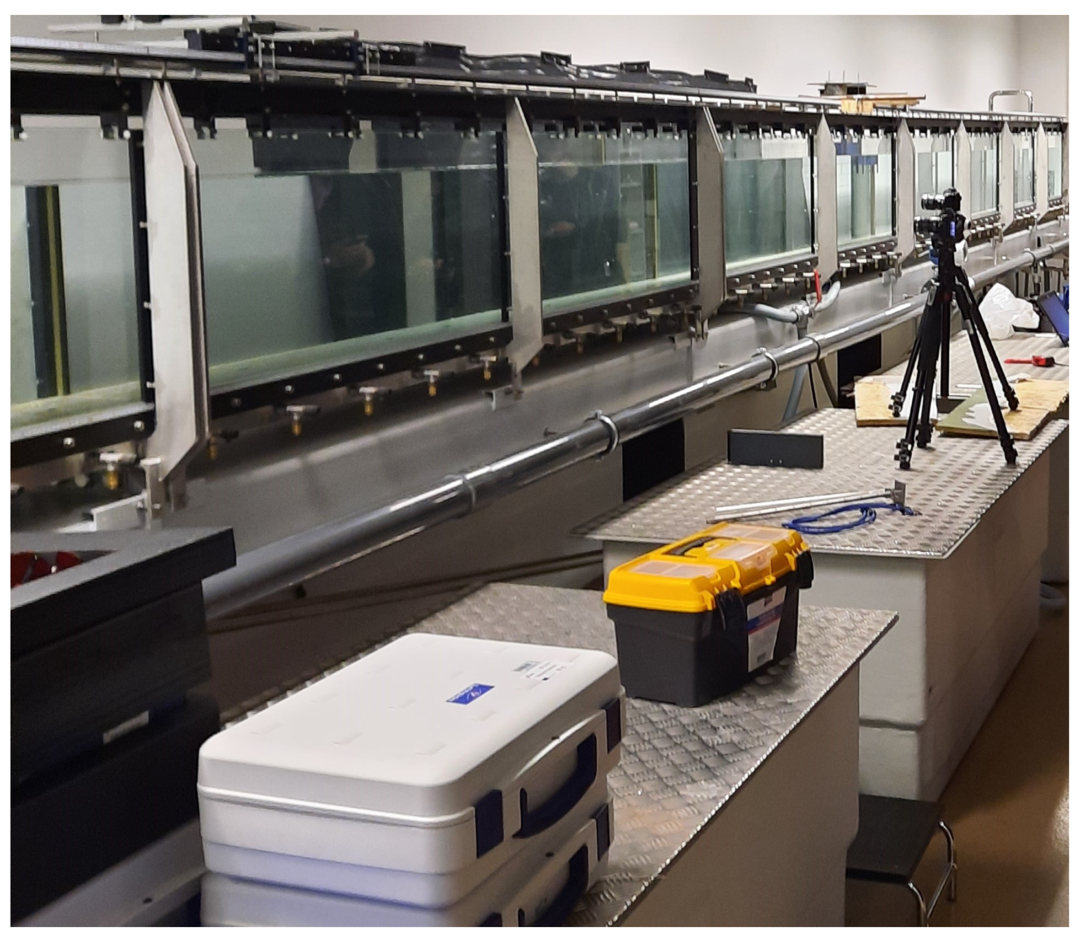
The experimental setup was the same as in our previous research Holjević et al. [36] with the experimental flume of the Hydrotechnical Laboratory of the Faculty of Civil Engineering University of Rijeka being used to measure the drag coefficient $c_d$ of MP particles settling in flowing water (Figure 1). The channel is 12.5 m long, with a rectangular cross-section of 0.309 m × 0.450 m. The flow rate in the channel was 72.0 m³/h, with a water depth approximately equal to 41 cm. The geometric and kinematic characteristics of the flow are controlled by a pump, a downstream weir, and the slope of the channel. The weir is positioned 12.0 m from the beginning of the flume and 7.5 m downstream from the dosing ramp. The slope of the experimental flume was set to zero.

The water used in the experiment was fresh water from the public water supply system, with a temperature of approximately 15 $°$C. In salt water like seas and oceans, MP particles would behave differently, since a higher density of media reduces the resultant weight force and, consequently, prolongs the particles’ total settling time. However, these effects do not influence the drag coefficient, the assessment of which is the aim of this research.

MP particles were produced by using a high-precision 3D printer with a minimum sample size of 0.4 mm and a precision of up to 32 microns. Using a printer for the production of MP particles ensures control over sample geometry and establishes the repeatability of the experiment. The same printer was also used to produce the dozing ramp, which was utilized for particle insertion into the water stream without significant linear and angular momentum and with minimized surface tension influence.

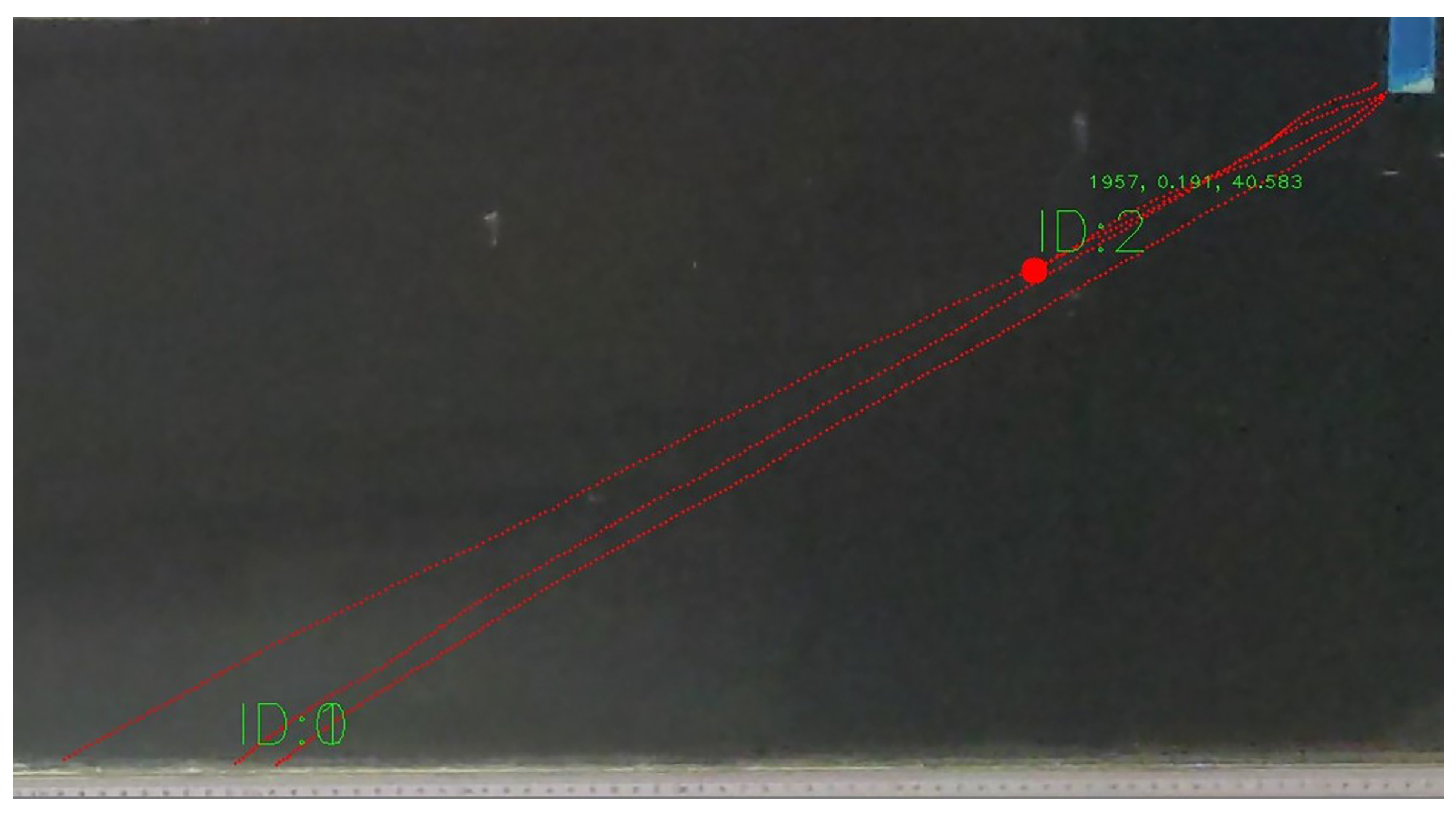
The entire particle settling process was recorded using video equipment and the analysis of video material was conducted using Open Source Computer Vision Library (OpenCV) version 4.5.5 for Python. OpenCV is an open-source computer vision and machine learning software library used for image and video processing. The video analysis was performed for the purpose of extracting the timed trajectory of each MP particle (Figure 2).

The videos of each experimental run were recorded at 30 frames per second in UHD (ultra high-definition) video quality using a Samsung A53 camera (Samsung Electronics Co. Ltd., Suwon, South Korea). The camera was positioned 2.4 m from the flume and oriented perpendicularly to the flume glass wall. The camera was managed remotely to minimize external influences on the camera due to manual handling.

Particle tracking in the video analysis was achieved by using Mixture of Gaussians 2 (MOG2) background subtractor algorithm for motion detection and the marking of shadows on the background model of MP particles. The MOG2 history parameter (the number of previous frames that affect the background model) was set to 100 for 3D particles (spheres and cubes) and 130 for 2D particles (plates). The VarThreshold parameter (defining the separation between a pixel and the model) was varied between 300 and 1100, depending on the size of the MP particle, with smaller values used for smaller shapes. Higher values were also used for 2D particles due to the smaller visible area of the particle registered by the camera. The particle coordinates obtained with the video analysis were then corrected for parallax and light refraction errors.

2.4. Drag Coefficient Model

The settling velocity of a particle in a fluid is influenced by both fluid properties (density and viscosity) and particle properties (density, size, shape, and surface texture). The functional relationship between these factors is generally not well quantified. Hence, empirical curves derived from laboratory experiments are typically proposed. When a particle is introduced into a Newtonian fluid with lower density, it will experience an initial acceleration driven by its own weight. The fluid’s resistance to deformation, which is transmitted to the particle through surface drag and pressure disparities across it, generates forces that resist the particle’s movement. These forces depend on the velocity and the acceleration of the particles [37].

The most influential forces on the MP settling process are buoyancy-adjusted particle weight $F_g$ and resistance force $F_d$, which can be written as:

$$\overrightarrow{F_g}=({\rho }_p-{\rho }_f)V_p\overrightarrow{g},$$

(4)

$$\overrightarrow{F_d}=\frac{1}{2}·c_d\left({\mathrm{Re}}_{\mathrm{p}}\right)·{\rho }_f·A_p·\overrightarrow{v_r}\left|\overrightarrow{v_r}\right|,$$

(5)

where ${\rho }_f$ is density of the fluid, ${\rho }_p$ is the density of solid particles, $V_p$ is particle volume, $\overrightarrow{g}$ is gravitational acceleration, $c_d$ is dimensionless particle drag coefficient, $R{e}_p$ is local Reynolds number, $A_p$ is the projection of the particle surface in the flow direction, and $\overrightarrow{v_r}$ is the relative velocity of the particle. Reynolds number Re depends on the relative magnitude of the inertial and viscous forces, which can in its local form be written as:

$${\mathrm{Re}}_{\mathrm{p}}=\frac{|\overrightarrow{v_r}|d}{\nu },$$

(6)

where d is characteristic particle length, $v_r$ is particle velocity relative to fluid velocity, and $\nu$ is kinematic fluid viscosity [9]. Taking into account Newton’s second law, the sum of the net forces can be written as:

$${\rho }_p{V}_p\overrightarrow{a_p}=\overrightarrow{F_g}+\overrightarrow{F_d},$$

(7)

with $\overrightarrow{a_p}$ being particle acceleration.

Disregarding the particle and fluid movement in the lateral axis y (perpendicular to both vertical axis and fluid flow direction axis) allows us to decompose the above equation into two equations corresponding to the two important dimensions, x and z:

$${\rho }_p{V}_p{a}_{p,x}=\frac{1}{2}·c_d\left({\mathrm{Re}}_{\mathrm{p}}\right)·{\rho }_f{A}_p·(v_{f,x}-v_{p,x})|v_{f,x}-v_{p,x}|,$$

(8)

and

$${\rho }_p{V}_p{a}_{p,z}=\frac{1}{2}·c_d\left({\mathrm{Re}}_{\mathrm{p}}\right)·{\rho }_f{A}_p·(v_{f,z}-v_{p,z})|v_{f,z}-v_{p,z}|+|\overrightarrow{F_g}|.$$

(9)

Combining the above two equations, we can express the drag coefficient as:

$$c_d=\frac{-2({\rho }_p-{\rho }_f)V_p\left|\overrightarrow{g}\right|}{{\rho }_f{A}_p·((v_{f,x}-v_{p,x})|v_{f,x}-v_{p,x}|·\frac{a_{p,z}}{a_{p,x}}-(v_{f,z}-v_{p,z})|v_{f,z}-v_{p,z}|)},$$

(10)

and the local particle Reynolds number can be calculated as:

$${\mathrm{Re}}_p=\frac{\sqrt{{(v_{f,x}-v_{p,x})}^2+{(v_{f,z}-v_{p,z})}^2}·d}{\nu },$$

(11)

where $v_{f,x}$ and $v_{f,z}$ are local fluid velocities in x and z direction and $v_{p,x}$ and $v_{p,z}$ are local particle velocities in x and z direction.

By capturing the complete particle settling process (namely particle positions $x\left(t\right)$ and $z\left(t\right)$), which was achieved by video recording and software analysis, and then using the Equations (10) and (11), it is possible to calculate the local values of the Reynolds number ${\mathrm{Re}}_p$ and drag coefficient $c_d$ along the entire trajectory of a particle.

2.5. Velocity Field

To calculate the local Reynolds number ${\mathrm{Re}}_p$ (11), it is necessary to know the difference between the velocity of the particle and the velocity of water. Therefore, it is required to determine velocity field for the water flowing in the experimental flume. For this purpose, a numerical simulation of the flow inside the flume was performed using OpenFOAM software (version v2012). CfMesh was used to create a numerical mesh, which includes refinements in zones near the particle input ramp and downstream ending weir. As part of the OpenFOAM software package, simpleFoam solver was used, which is commonly used for steady-state, incompressible turbulent flow simulations. The initial velocity at the inlet boundary was set to 0.17 m/s, which is the value measured by a flow meter during the experiments. The outlet boundary was represented with the Neumann boundary condition (zeroGradient in OpenFOAM). The top surface of the domain was treated as a free-slip boundary, whereas at the bottom, input ramp, and side wall surfaces, a no-slip condition was applied. The simulation of turbulence flow was computed using the k-epsilon turbulence model as implemented in OpenFOAM.

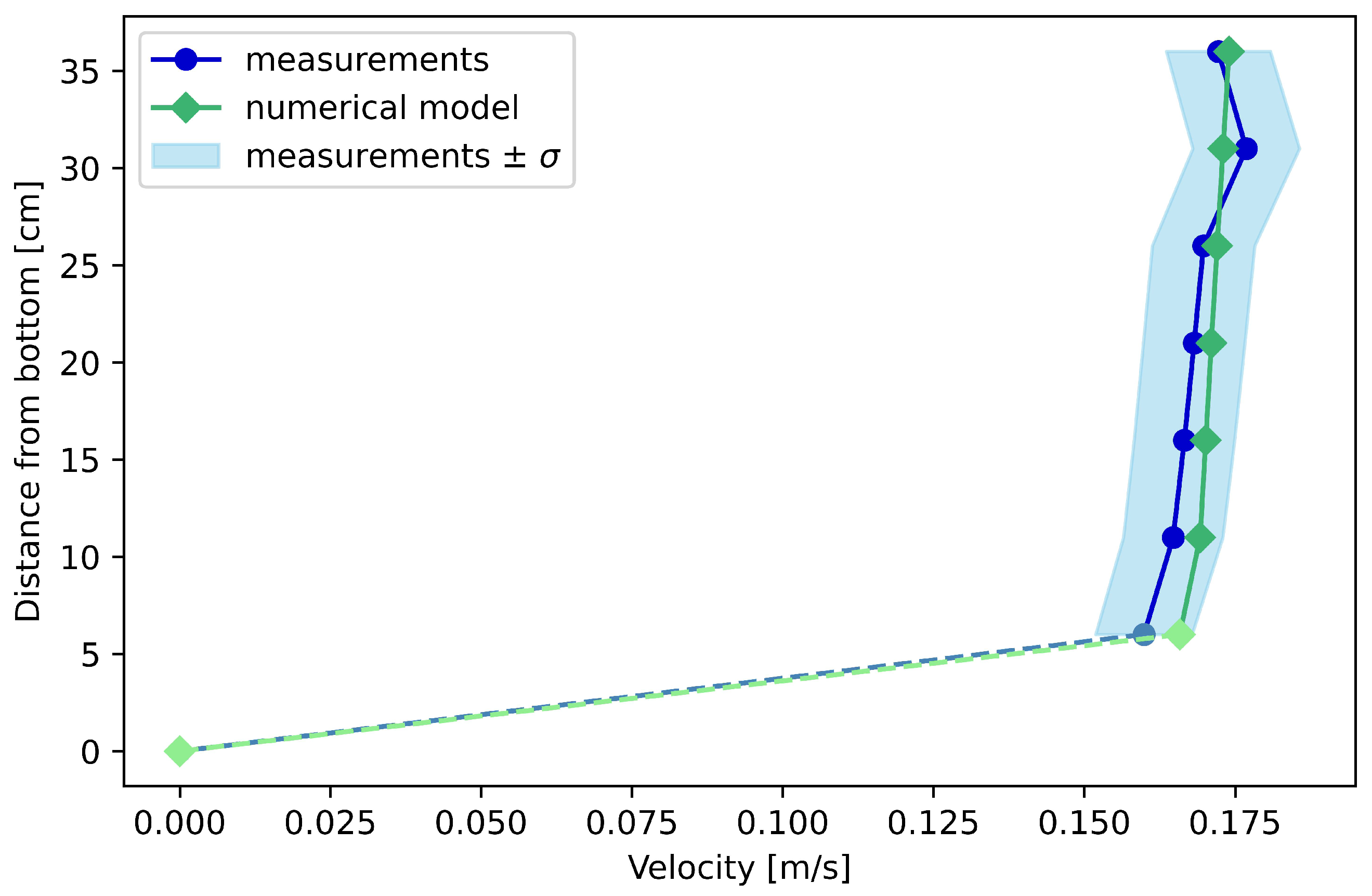
The resulting velocity field obtained by the numerical model was compared with the results of the experimental measurements, which were collected using a Nortek Vectrino velocimeter [36]. The measurement was performed on a total of 7 vertically distributed points in the central axis of the flume (vertical points at a distance of 5 mm from each other, starting with a point at 5 mm from the bottom of the flume). The comparison of velocity profiles is given in (Figure 3). Due to technical limitations of the Vectrino device, the flow velocity near the bottom could not be measured, so it was linearly extrapolated, conforming to the bottom no-slip condition. From the data obtained with the numerical model (

Table 3. Measured and simulated flow velocity in the experimental flume, 0.5 m downstream of the input ramp.

Distance from Bottom [cm]	Measurements		Numerical Model
	${\mathit{v}}_{\mathit{f},\mathit{x}}$ [m/s]	$\mathit{\sigma }$ [m/s]	${\mathit{v}}_{\mathit{f},\mathit{x}}$ [m/s]
36	0.172234	0.00861	0.173998
31	0.17684	0.00884	0.173006
26	0.169773	0.00848	0.172026
21	0.16821	0.00841	0.171069
16	0.16659	0.00832	0.170149
11	0.164735	0.00823	0.169191
6	0.159888	0.00799	0.165824

), it can be observed that the differences between the measured and computed velocity values are smaller than the standard deviation of the measurements.

Due to the fact that the deviations between the velocity measurements and numerical model are within the limits of standard deviation, the estimation of the particle drag coefficient was conducted by using the velocity field obtained with the OpenFOAM numerical model.

3. Results and Discussion

The trajectories of the spheres, cubes, and square plate settling particles were recorded, and on the basis of this data, $c_d$ and ${\mathrm{Re}}_p$ values were calculated using formulae (10) and (11). Since these formulae use particle velocities $\overrightarrow{v_p}$ and accelerations $\overrightarrow{a_p}$, those were computed analytically (as first and second time derivatives) from the mean of the polynomial regressions of the trajectories of all particles in a shape/size group. The measured trajectories needed to be statistically stabilized to provide balance with the steady (i.e., time-averaged) flow velocity field used in the formulae, and mean regression was used as an averaging tool for this purpose. Furthermore, it should be noted that the used experimental technique cannot detect lateral movements of particles (in the direction of the y axis, i.e., orthogonal to the x-z plane), and as a result, particle trajectories are not captured entirely accurately. Trajectories are observed only in the x-z plane; therefore, the condition of balance of forces in (7) is not fully satisfied. There are also limitations of the particle tracking method precision manifesting through the discretization of the measured trajectories in the spatial and temporal domain, as well as through the imperfections of the OpenCV video analysis of the particle motion.

Significant improvements regarding the $c_d$ assessment methodology could only be made by using additional video camera(s) and recording particle movement in both the x-z and x-y planes. This would allow the detection of lateral particle movement and the addition of the velocity components in the y direction in the $c_d$ calculation procedure (8) and (9). However, this would not produce a significant increase of $c_d$ assessment accuracy per se, since trajectory recording would need to be coupled with synchronous unsteady 3D measurements of the velocity field, which was entirely unfeasible in context of this research.

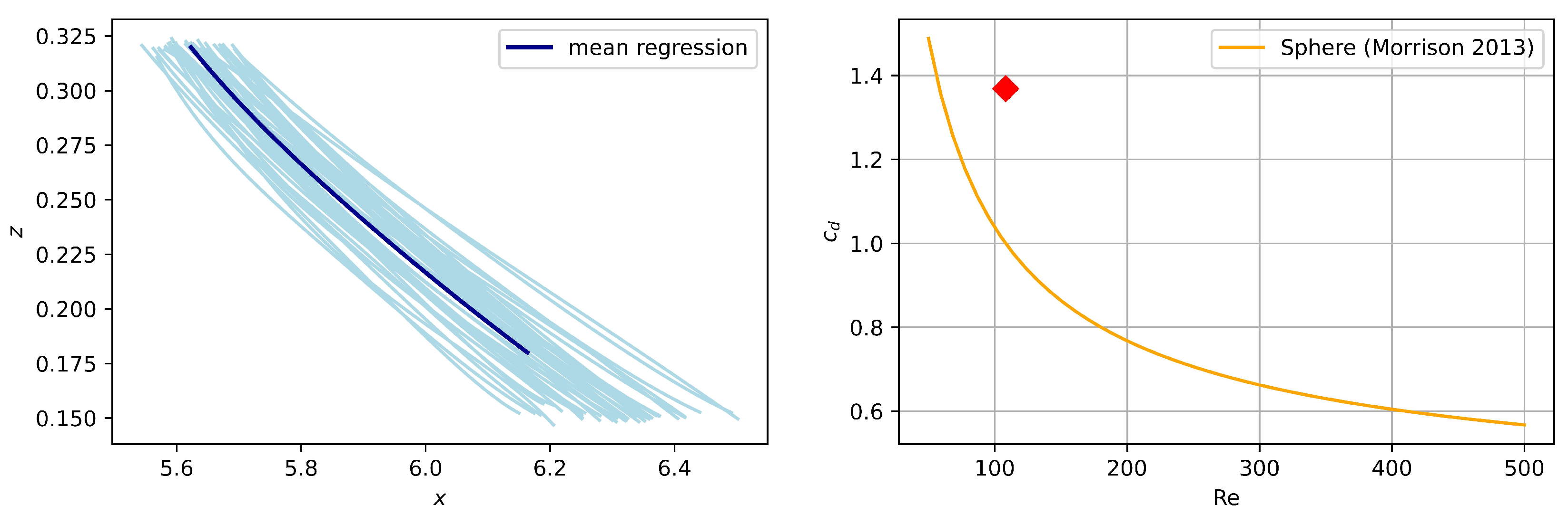
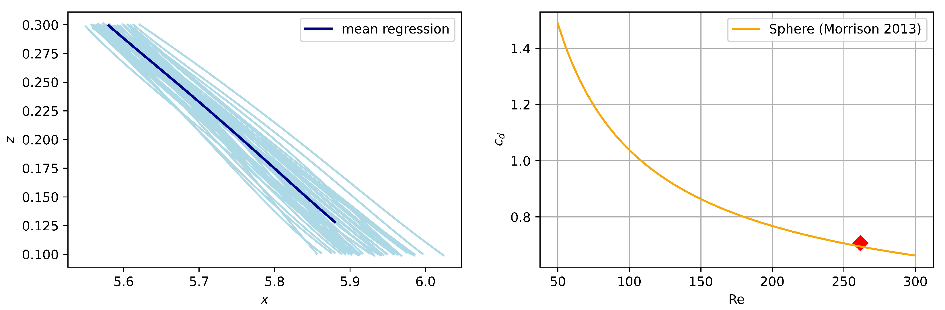
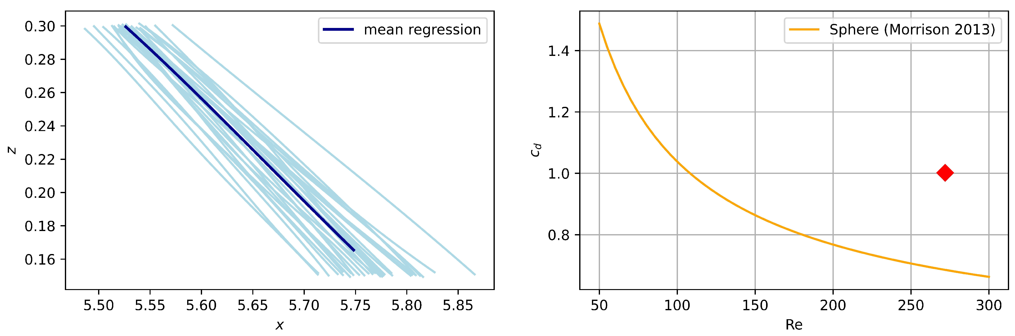
Due to all of the above, statistical analysis was necessary for the calculation of the drag coefficient. For each particle size/shape type, 40 trajectories were smoothed using regression on the data obtained by OpenCV analysis, and mean regression trajectory was adopted for further calculation. Of all calculated $({\mathrm{Re}}_p,c_d)$ values corresponding to the points of the mean regression trajectory, the median one (red diamond in figures below) is taken as representative.

The regressions of the trajectories and the calculated $c_d\left(\mathrm{Re}\right)$ values are displayed in Figure 4 (spheres), Figure 5 (cubes), and Figure 6 (plates) for particles with the characteristic length $d=3$ mm.

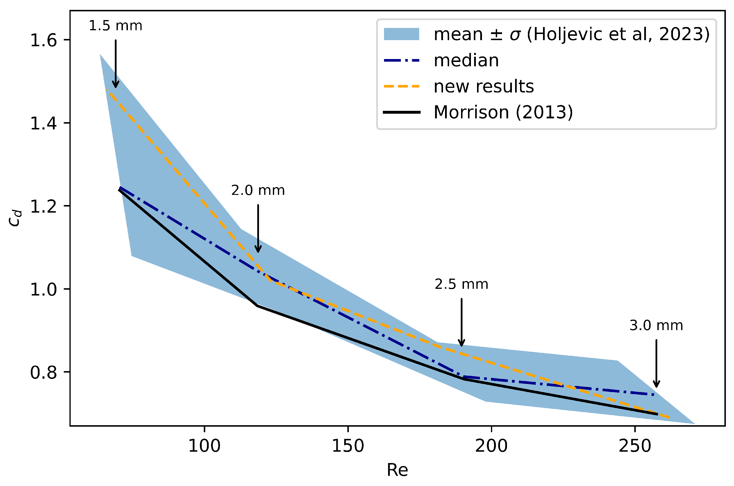
Trajectory-based $c_d\left({\mathrm{Re}}_p\right)$ values for spheres, obtained from the experimental data and the proposed formulae, were compared with previous results [36,38] for validation. The comparison given in Figure 7 includes the $c_d\left({\mathrm{Re}}_p\right)$ curve according to [38], shown with a black line; the results of previous research [36], presented with a blue dash-dotted line, with the light blue area representing $c_d\left({\mathrm{Re}}_p\right)$ in the range of the mean value ± standard deviation $\sigma$; whereas the dashed orange line shows the results of newly proposed empirical model. This result shows good agreement with both previous results and the literature [38] and, as such, allowed for a conclusion that the proposed empirical model is a valid method of experimental drag coefficient assessment. Further analyses were conducted with the use of the validated empirical model.

Finally, the complete results of the experimental assessment of ($c_d,{\mathrm{Re}}_p$) values for the three used MP particle shapes are given in

Table 4. ${\mathrm{Re}}_p$ and $c_d$ values for MP particles in the shapes of sphere, cube, and square plate.

Particle Shape	d [mm]	Median ${\mathbf{Re}}_{\mathit{p}}$ [-]	Median ${\mathit{c}}_{\mathit{d}}$ [-]
Sphere	3.0	262	0.69
	2.5	182	0.86
	2.0	123	1.02
	1.5	66	1.48
Cube	3.0	276	0.97
	2.5	207	1.01
	2.0	133	1.31
	1.5	78	1.60
Square plate	3.0	106	1.37
	2.5	93	1.39
	2.0	72	1.4
	1.5	54	1.5

.

The obtained median values of Re and $c_d$ for the examined particle shapes were used for establishing the regression models shown in Figure 8. The values of the calculated drag coefficient for 3D particles (sphere and cube) range from 0.69 to 1.48 for sphere and from 0.97 to 1.60 for cubic particles, with the Reynolds number ranging from 66 to 276. As expected, the concave shape of the curve is preserved for both sphere and cubic particles. An increase in $c_d$ values for cube particles when compared to $c_d$ values for spheres is an expected consequence of less efficient hydro-dynamical properties. The results for plate shape particles span a relatively small range of Re numbers, from 54 to 106, with $c_d$ values ranging from 1.37 to 1.5, and, as such, do not allow for strong conclusions. Certainly, it can be noted that they show $c_d$ values greater than those of spheres, which is expected. A relative increase in $c_d$ is stronger for cube particles (3D) than for plate shape particles (2D), which can also be noted in the linear coefficient of the regression function: its value for the cubes ($-1.29\times {10}^{-2}$) is greater than for plates ($-9.6\times {10}^{-3}$), which is manifested in the steepness of the regression curve.

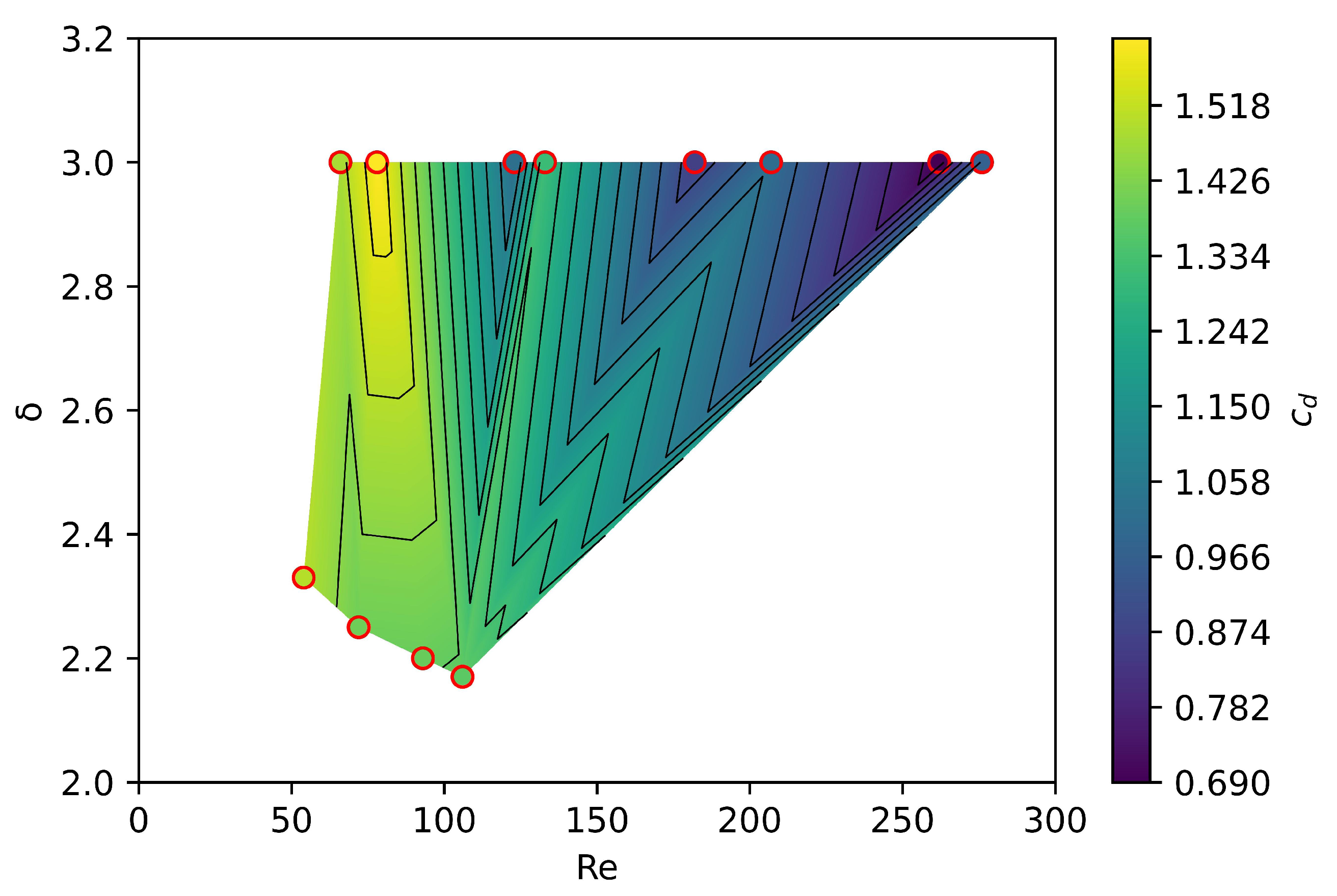
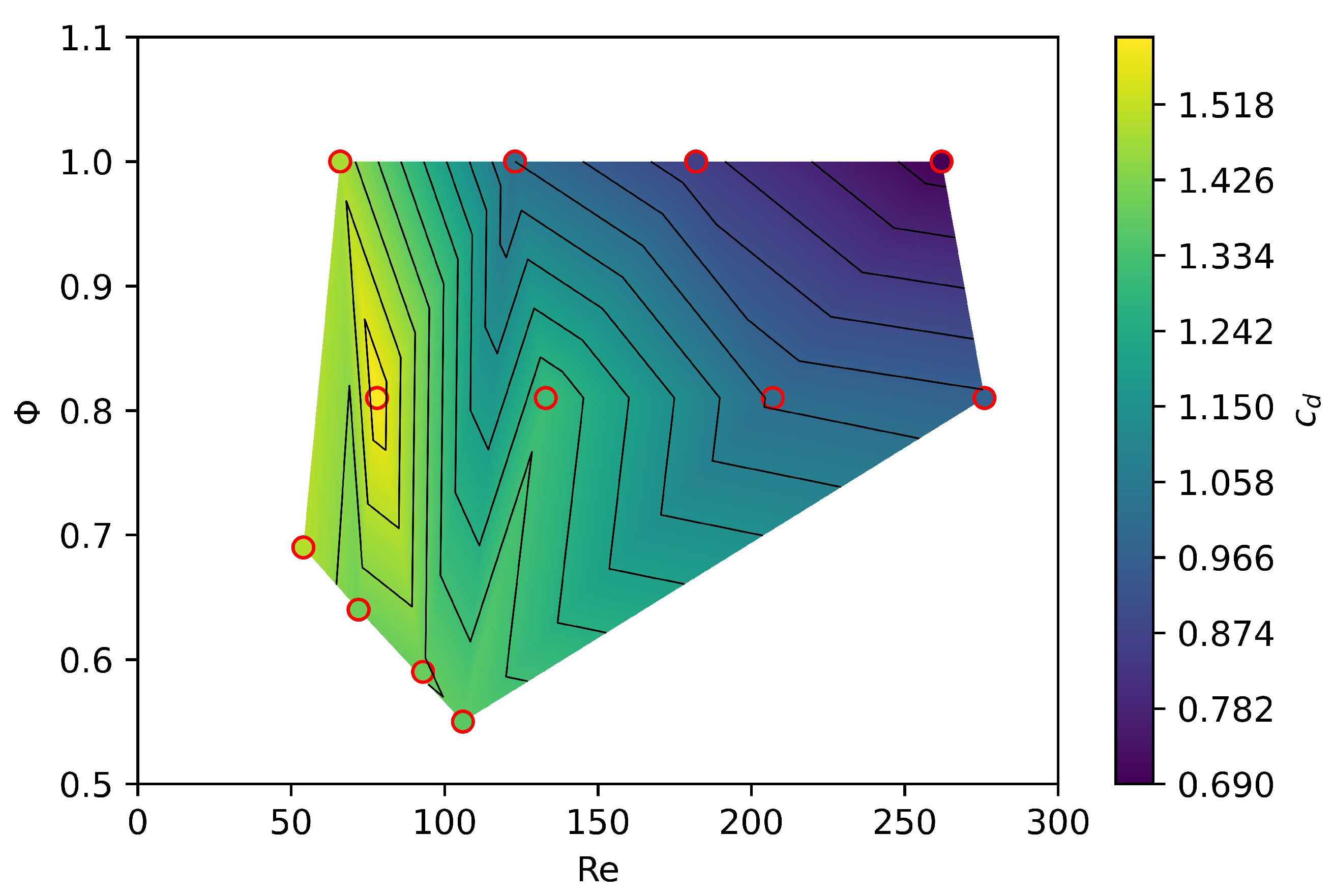
Shape Parameterization Based Drag Coefficient Model

The results given in Table 4 were used to produce a model for estimating the drag coefficient $c_d$ on the basis of shape parameters. For this purpose, particle dimensionality $\delta$ (Figure 9) and particle sphericity $\varphi$ (Figure 10) were put in relation to the obtained $c_d\left({\mathrm{Re}}_p\right)$ values for all sphere, cube, and plate particles (12 points in total). In these figures, the drag coefficient $c_d$ values are represented with a color gradient.

Sphericity $\varphi$ shows better practical implementation due to the fact that it can distinguish between 3D objects of different shapes like spheres ($\varphi =1$) and cubes ($\varphi =0.81$). Dimensionality $\delta$, however, showed a lack of ability to differentiate such shapes and, therefore, it appears to be of limited use for this type of functional representation. This is clearly visible in Figure 9, which shows a rather inconsistent $c_d({\mathrm{Re}}_p,\delta )$ model for $\delta \approx 3$.

The model given in Figure 9 and Figure 10 should be primarily understood as the demonstration of a possibility of forming shape-based models for drag coefficient estimation. With this in mind, it should be noted that, for them to be more useful, such models should be founded on a larger data set.

As a further illustration of the potential usefulness of these models, a regression model was fitted to the experimental data. The resulting empirical formula, using Re and $\varphi$ as parameters for producing $c_d$ values, is:

$$c_d(\mathrm{Re},\varphi )=0.00001{\mathrm{Re}}^{2.03752}+0.97108{\varphi }^{0.51593}-0.00839\mathrm{Re}\varphi +1.01877.$$

(12)

The formula should be used for Re values in the range of 50 to 280 and $\varphi$ values in the range of 0.55 to 1. The root mean square error (RMSE) of the $c_d$ values produced by this regression model is 0.072.

These results suggest the need for further research of the settling behaviour of MP particles of various shapes, where a greater number of different asymmetrical cuboid particle shapes should be taken into account. In planned continuation of this research, plate particles with different thickness will be observed and, consequently, a wider range of shape parameter values will be covered.

Both used shape descriptors show reasonably good practicality for the analyzed particle shapes, with some limitations present for both parameters. It should be taken into account that the choice of an adequate shape descriptor can vary significantly with respect to type of MP analyzed. Different types of MP can result in various particle shapes, thus imposing the need for different or additional shape descriptors. These might include parameters like aspect ratio, circularity, or the fractal dimension. It is also important to consider the limitations and potential sources of model error associated with each shape descriptor. For a more comprehensive analysis, future research should test the usage of other specific shape descriptors in combination with sphericity and dimensionality.

4. Conclusions

The transport and settling process of microplastics (MP) is highly influenced by particle size and shape. The shape of MP is particularly interesting due to the fact that MP particles in nature appear in various forms, with film (plate) particles being one of the most common shapes of MP in aquatic environments. The influence of shape in the transport and settling of MP particles is modeled through the drag coefficient $c_d$; thus, an empirical methodology for its assessment was proposed in this paper.

An experimental analysis of the settling behavior of flat square particles and 3D cubic particles in flowing water was conducted, in which the settling trajectories of such particles of various sizes were experimentally measured and used for calculating the drag coefficient $c_d$ in relation to the Reynolds number Re. The water velocity field needed for this calculation was reconstructed as a combination of the CFD model and experimental measurements performed with a Nortek Vectrino velocimeter. The resulting $c_d\left({\mathrm{Re}}_p\right)$ values were correlated with two shape parameters, sphericity $\varphi$ and a newly proposed shape descriptor, dimensionality $\delta$, in an easy-to-use model for shape-based $c_d$ estimation. Sphericity $\varphi$ has shown to be a more useful parameter for this kind of analysis, whereas other parameterization methods still need to be explored.

The used methodology produces good agreement with previous research and illustrates the capabilities of the proposed experimental approach for the precise calculation of local Re and $c_d$. The resulting shape sphericity-based model for MP particle $c_d$ estimation shows potential for practical utility, although it is obvious that further research regarding cuboid-shape particles with different thicknesses is needed.

Future studies should also consider the use of additional or different shape descriptors for various types of microplastics. Such dimensionless shape parameters enable the comparison of different MP particle shapes, regardless of their size. In order to investigate the impact of morphology on the MP particles’ behavior in water, we should quantify their morphology in a standardized way. Another approach, alternative to the one used in this research and also worth exploring, would be to normalize the total area of the particle, as it is one of the most important parameters influencing MP behavior and ecotoxicological effects.