


Power Prediction Method for Ships Using Data Regression Models


Abstract
:1. Introduction
2. Methods
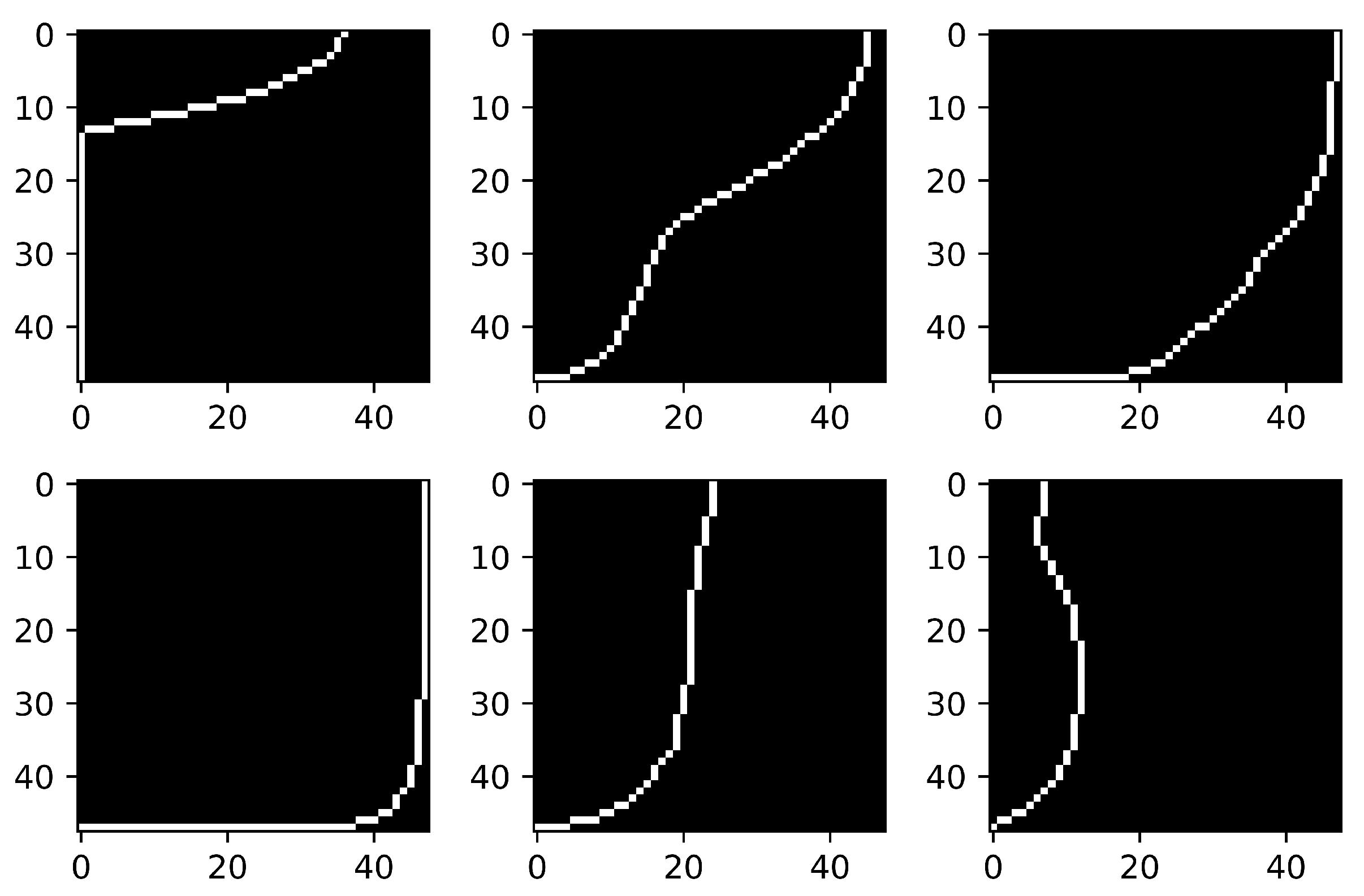
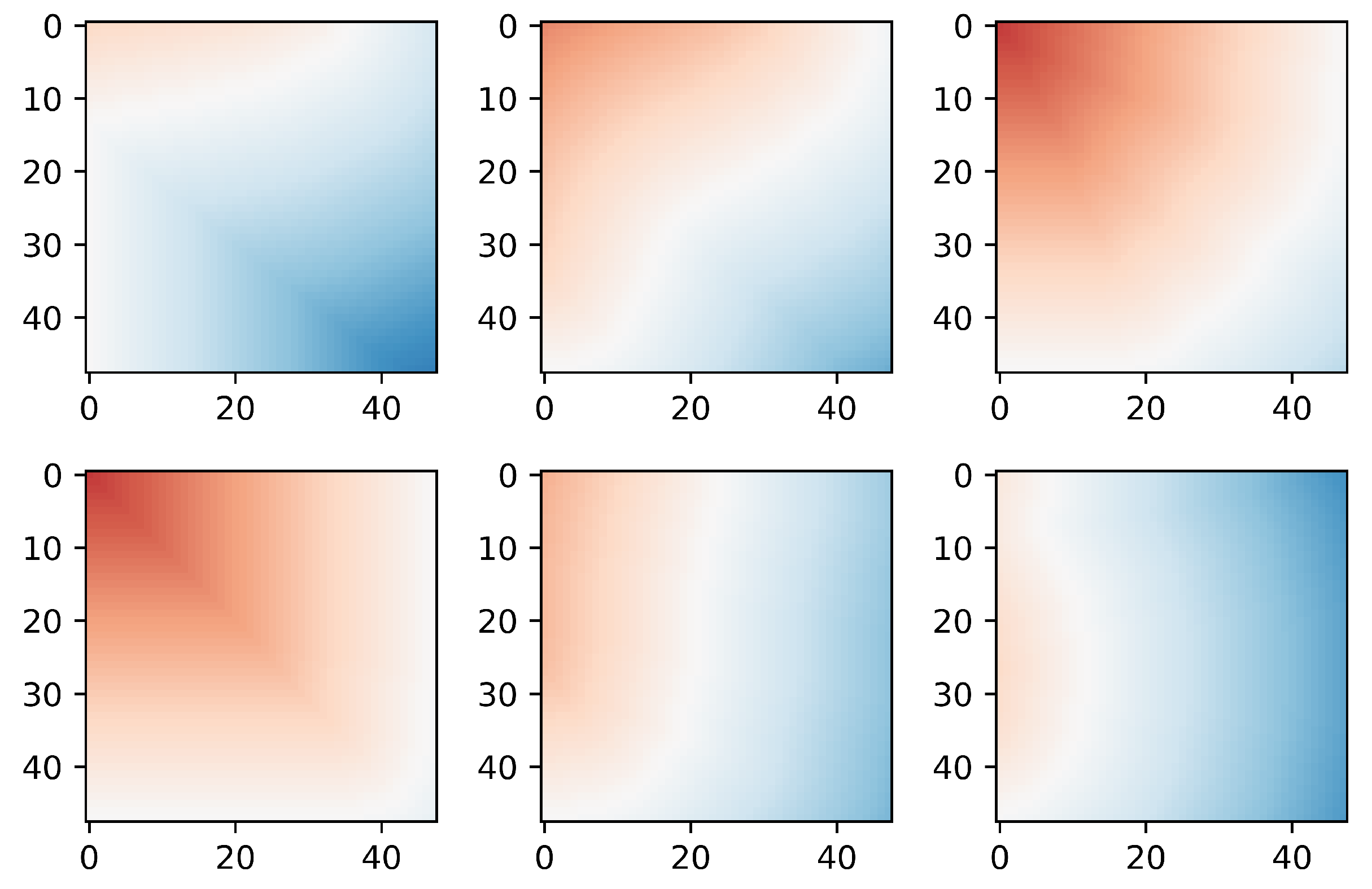
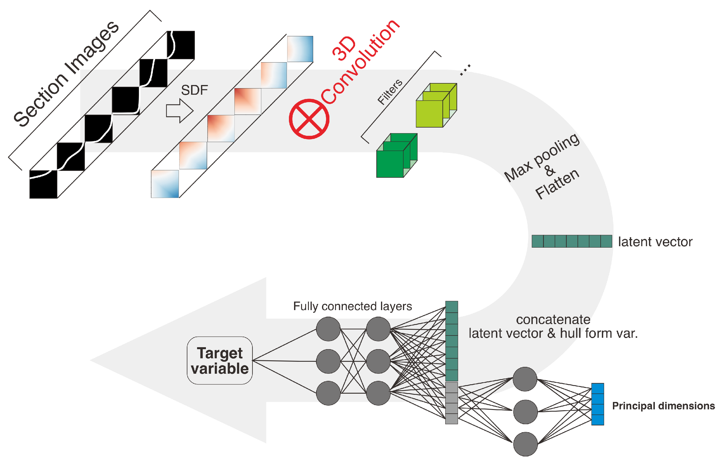
2.1. Hull Geometry Representation
2.2. Model Construction
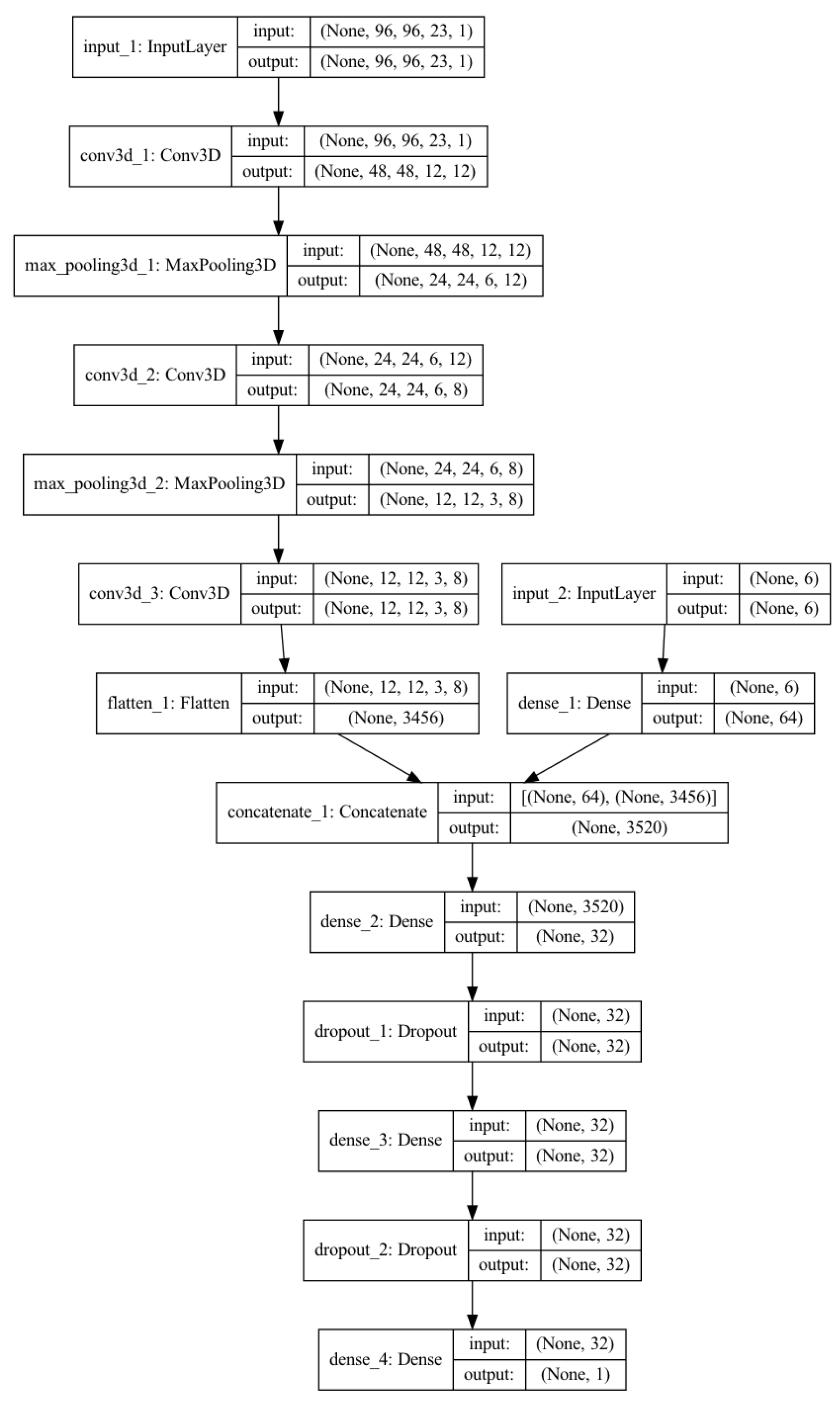
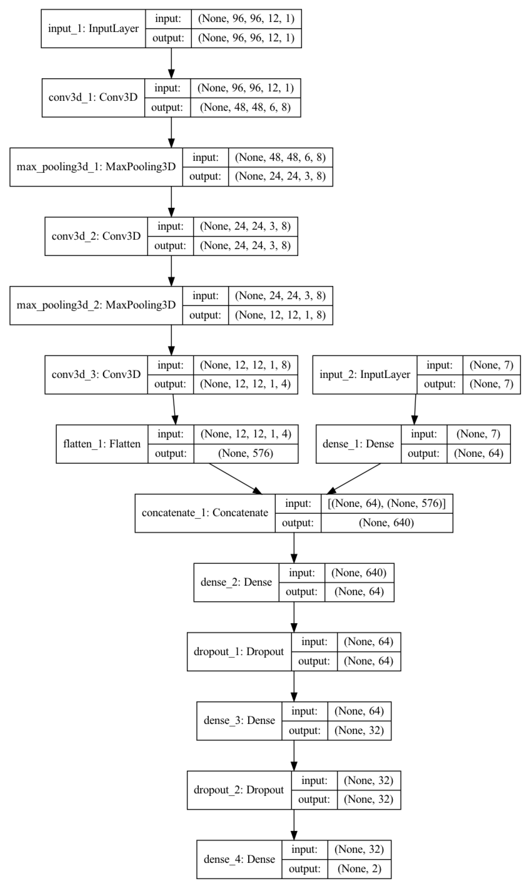
2.2.1. CNN Model
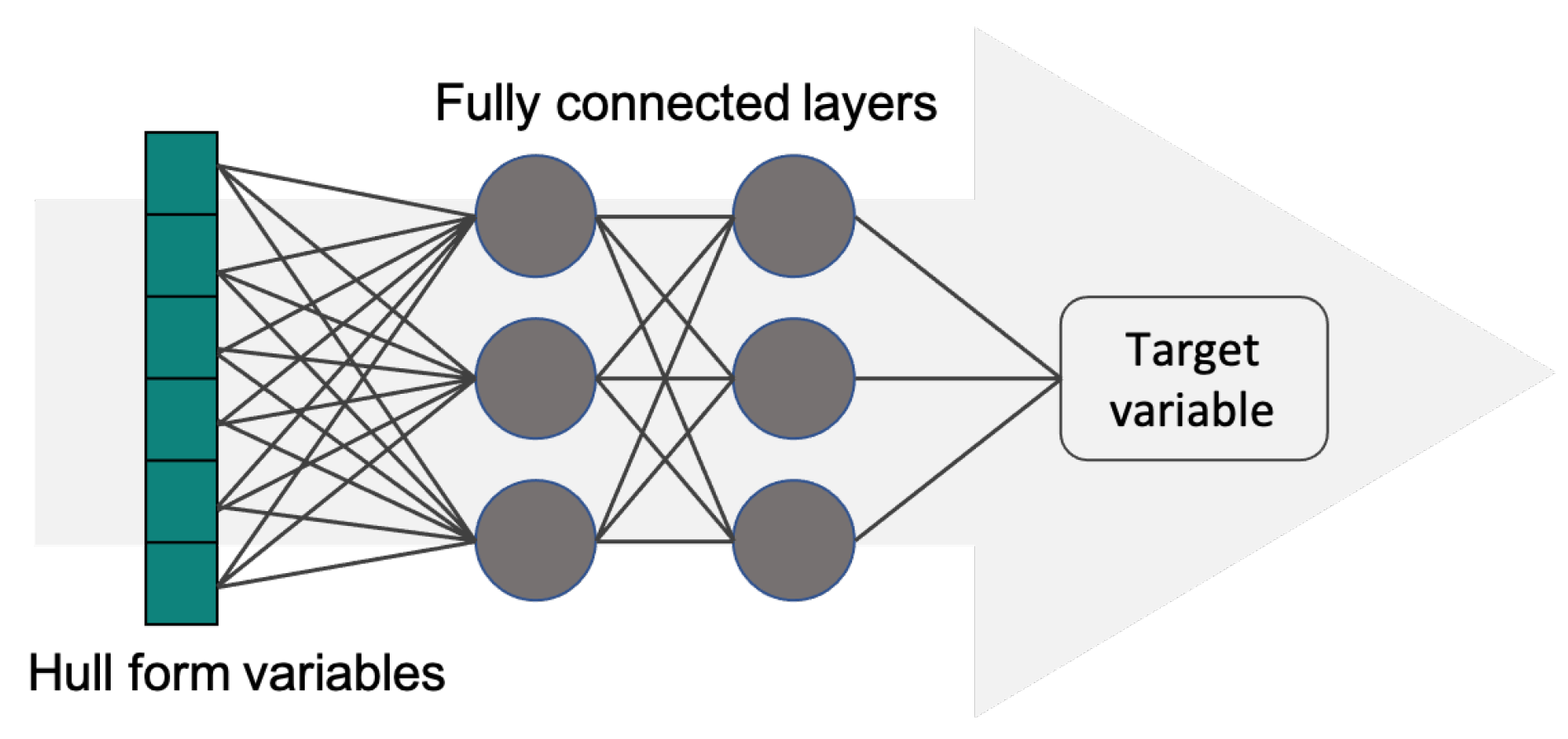
2.2.2. MLP Model
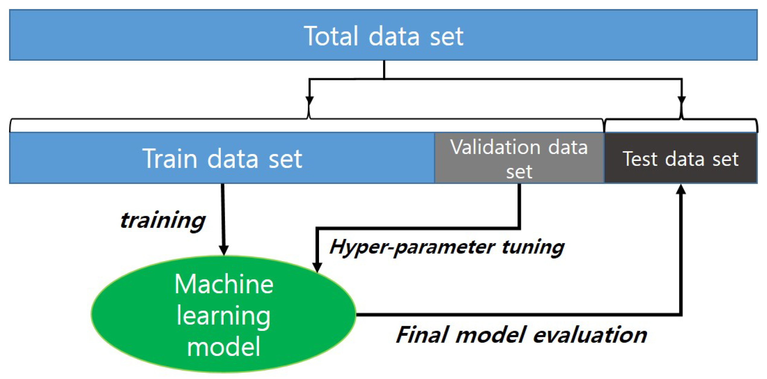
2.3. Training Data
3. Prediction Results Regarding the Ship Hydrodynamic Characteristics
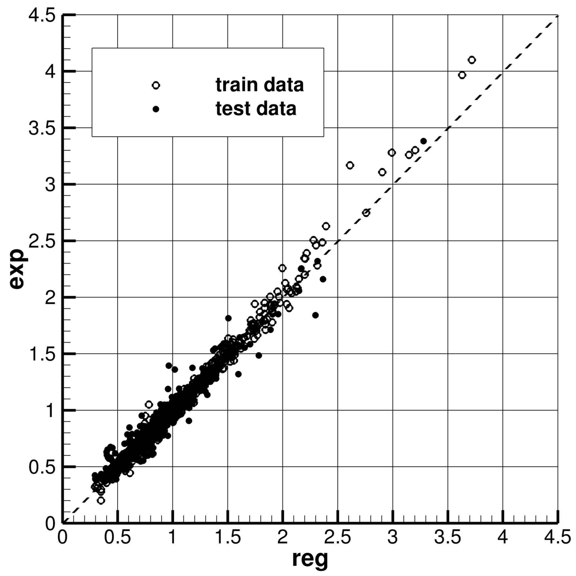
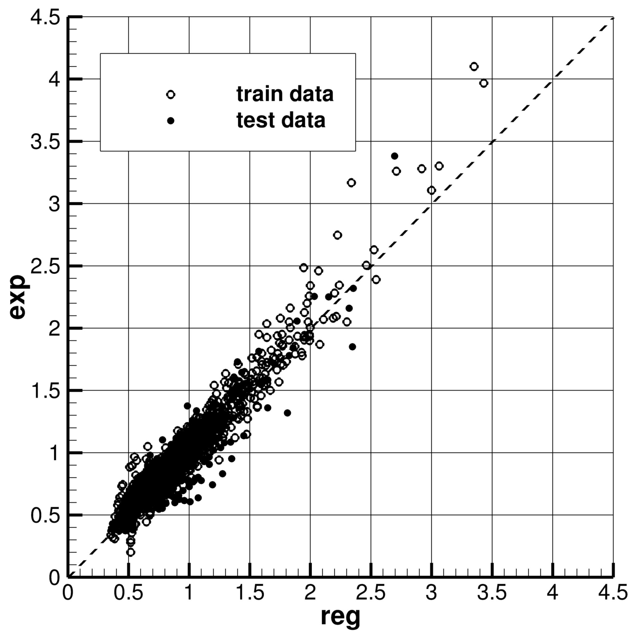
3.1. Residuary Resistance Coefficient
3.1.1. CNN Model
3.1.2. MLP Model
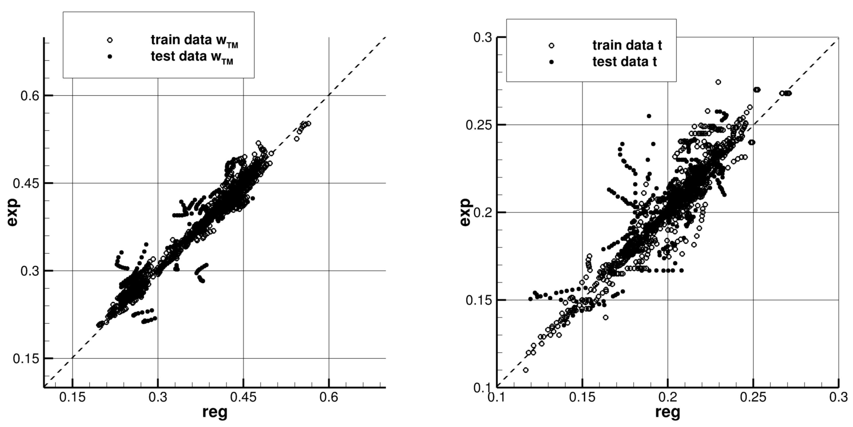
3.2. Wake and Thrust Deduction Fractions
3.2.1. CNN Model
3.2.2. MLP Model
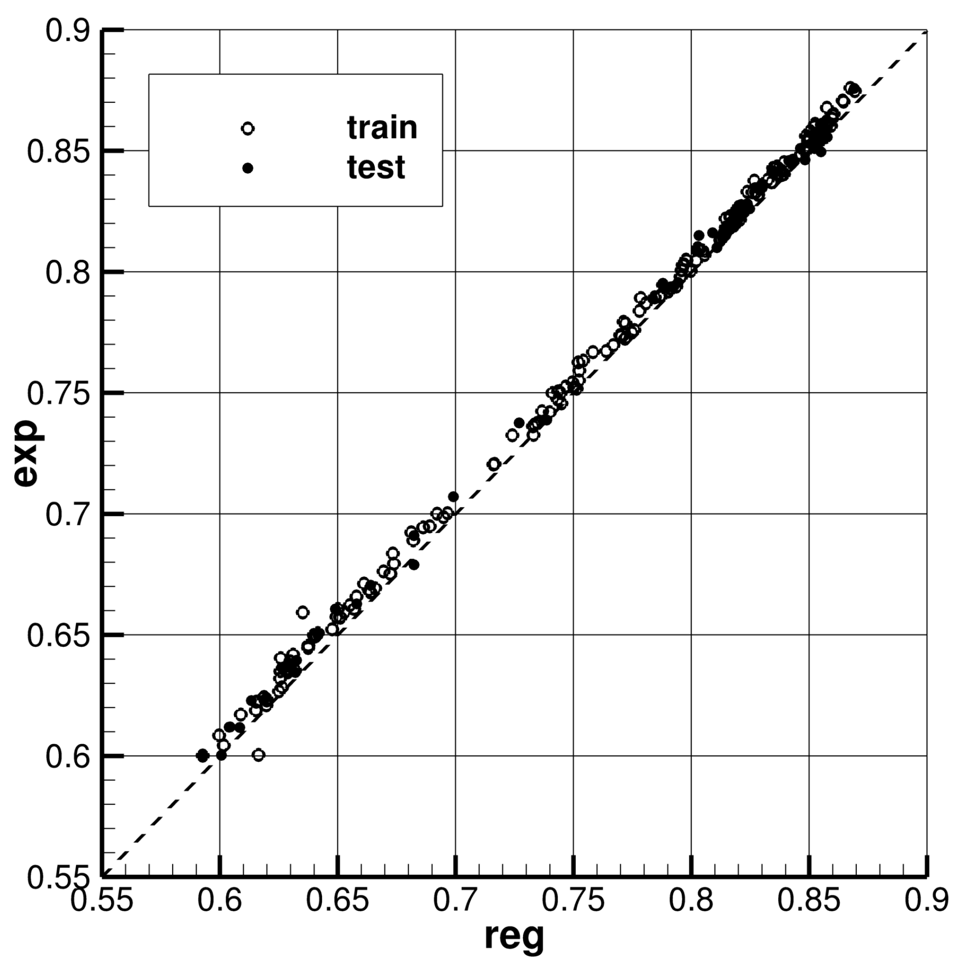
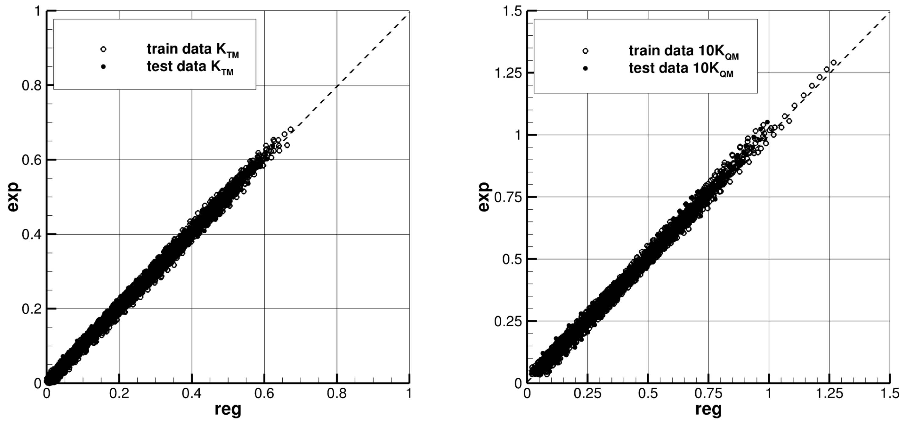
3.3. POW Characteristics
3.4. Summary of the Final Models
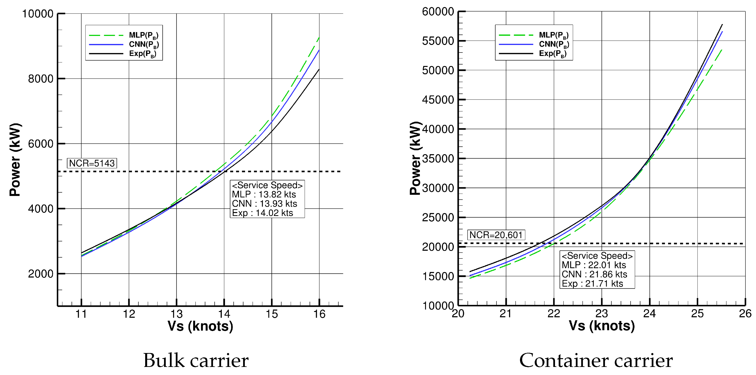
4. Power Prediction
4.1. Performance Prediction Method
4.2. Case Study
5. Concluding Remarks
- Development of MLP models for , , and t
- Development of CNN models for , , and t
- -
- Image-based hull form representation using a signed distance function
- Development of MLP models for and
- Development of power prediction method using the developed regression models
Author Contributions
Funding
Institutional Review Board Statement
Informed Consent Statement
Data Availability Statement
Conflicts of Interest
Nomenclature
| L | L indicates (Length between perpendiculars) |
| B | Breadth |
| T | Draught |
| Block coefficient | |
| Block coefficient of after body | |
| Longitudinal center of buoyancy | |
| ∇ | Displacement volume |
| Bulbous bow length | |
| Propeller diameter | |
| Z | Number of propeller blades |
| Expanded blade area ratio | |
| Pitch ratio at 0.7R | |
| Mean pitch ratio | |
| Wetted surface area of bare hull | |
| Bilge keel area | |
| Projected area of ship above the water line to the transverse plane | |
| Mass density of air | |
| Mass density of water | |
| Froude number | |
| Reynolds number | |
| J | Propeller advance ratio |
| Residuary resistance coefficient | |
| Wake fraction | |
| t | Thrust deduction fraction |
| Thrust coefficient | |
| Torque coefficient | |
| Total resistance | |
| Total resistance coefficient | |
| Frictional resistance coefficient | |
| Incremental resistance coefficient for model ship correlation | |
| Air or wind resistance coefficient | |
| Brake power | |
| Relative rotative efficiency | |
| Transmission efficiency | |
| n | Propeller frequency of revolution |
| Symbols for subscript | M: model, S: ship |
References
- Taylor, D.W. Speed and Power of Ships; Press of Ransdell: Washington, DC, USA, 1933. [Google Scholar]
- Gertler, M. A Reanalysis of the Original Test Data for the Taylor Standard Series; Navy Department the David W. Taylor Model Basin, Report 806; US Government Printing Office: Washington, DC, USA, 1954.
- Lap, A.J.W. Resistance (Fundamentals of ship resistance and propulsion). Int. Shipbuild. Prog. 1956, 3, 441. [Google Scholar] [CrossRef]
- Guldhammer, H.E.; Harvald, S.A. Ship Resistances Effect of Form and Principal Dimensions; Akademisk, Forlag: Copenhagen, Denmark, 1965. [Google Scholar]
- Holtrop, J.; Mennen, G.G.J. A statistical power prediction method. Int. Shipbuild. Prog. 1978, 25, 253. [Google Scholar] [CrossRef]
- Holtrop, J.; Mennen, G.G.J. An approximate power prediction method. Int. Shipbuild. Prog. 1982, 29, 166–170. [Google Scholar] [CrossRef]
- Holtrop, J. A statistical re-analysis of resistance and propulsion data. Int. Shipbuild. Prog. 1984, 31, 272–276. [Google Scholar]
- Kim, Y.C.; Kim, M.S.; Yang, K.K.; Lee, Y.Y.; Yim, G.T.; Kim, J.; Hwang, S.H.; Kim, K.S. Prediction of residual resistance coefficient of low-speed full ships using hull form variables and model test results. J. Soc. Nav. Arch. Korea 2019, 56, 448–457. [Google Scholar]
- Kim, Y.C.; Yang, K.K.; Kim, M.S.; Lee, Y.Y.; Kim, K.S. Prediction of residual resistance coefficient of low-speed full ships using hull form variables and machine learning approaches. J. Soc. Nav. Arch. Korea 2020, 57, 311–321. [Google Scholar]
- Cho, Y.I.; Oh, M.J.; Seok, Y.S.; Lee, S.J.; Roh, M.I. Resistance estimation of a ship in the initial hull design using deep learning. Korean J. Comput. Des. Eng. 2019, 24, 203–210. [Google Scholar] [CrossRef]
- Bertram, V.; Mesbahi, E. Estimating resistance and power of fast monohulls employing artificial neural nets. In Proceedings of the International Conference High Performance Marine Vehicles, Rome, Italy, 27–29 September 2004. [Google Scholar]
- Couser, P.; Mason, A.; Mason, G.; Smith, C.R.; von Konsky, B.R. Artificial neural networks for hull resistance prediction. In Proceedings of the Compit 2004, Siguenza, Spain, 9–12 May 2004. [Google Scholar]
- Yang, Y.; Tu, H.; Song, L.; Chen, L.; Xie, D.; Sun, J. Research on accurate prediction of the container ship resistance by RBFNN and other machine learning algorithms. J. Mar. Sci. Eng. 2021, 9, 376. [Google Scholar] [CrossRef]
- Cepowski, T. The prediction of ship added resistance at the preliminary design stage by the use of an artificial neural network. Ocean Eng. 2020, 195, 106657. [Google Scholar] [CrossRef]
- Liu, S.; Papanikolaou, A. Fast approach to the estimation of the added resistance of ships in head waves. Ocean Eng. 2016, 112, 211–225. [Google Scholar] [CrossRef]
- Liu, S.; Papanikolaou, A. Regression analysis of experimental data for added resistance in waves of arbitrary heading and development of a semi-empirical formula. Ocean Eng. 2020, 206, 107357. [Google Scholar] [CrossRef]
- Liu, S.; Papanikolaou, A. Improvement of the prediction of the added resistance in waves of ships with extreme main dimensional ratios through numerical experiments. Ocean Eng. 2023, 273, 113963. [Google Scholar] [CrossRef]
- Martić, I.; Degiuli, N.; Majetić, D.; Farkas, A. Artificial neural network model for the evaluation of added resistance of container ships in head waves. J. Mar. Sci. Eng. 2021, 9, 826. [Google Scholar] [CrossRef]
- Martić, I.; Degiuli, N.; Grlj, C.G. Prediction of added resistance of container ships in regular head waves using an artificial neural network. J. Mar. Sci. Eng. 2023, 11, 1293. [Google Scholar] [CrossRef]
- Yidiz, B. Prediction of residual resistance of a trimaran vessel by using an artificial neural network. Brodogradnja 2022, 73, 127–140. [Google Scholar] [CrossRef]
- Ichinose, Y.; Taniguchi, T. A curved surface representation method for convolutional neural network of wake field prediction. J. Mar. Sci. Technol. 2022, 27, 637–647. [Google Scholar] [CrossRef]
- Zhang, S. Research on the deep learning technology in the hull form optimization problem. J. Mar. Sci. Eng. 2022, 10, 1735. [Google Scholar] [CrossRef]
- Scholcz, T.; van Daalen, E. Surrogate-based multi-objective optimisation for powering and seakeeping. In Practical Design of Ships and Other Floating Structures; Springer: Singapore, 2021; pp. 477–492. [Google Scholar]
- Guerrero, J.; Cominetti, A.; Pralits, J.; Villa, D. Surrogate-based optimization using an open-source framework: The bulbous bow shape optimization case. Math. Comput. Appl. 2018, 23, 0060. [Google Scholar] [CrossRef]
- Bresenham, J.E. Algorithm for computer control of a digital plotter. IBM Syst. J. 1965, 4, 25–30. [Google Scholar] [CrossRef]
- Guo, X.; Li, W.; Iorio, F. Convolutional neural networks for steady flow approximation. In Proceedings of the 22nd ACM SIGKDD International Conference on Knowledge Discovery and Data Mining, San Francisco, CA, USA, 13–17 August 2016. [Google Scholar]
- He, K.; Zhang, X.; Ren, S.; Sun, J. Delving Deep into Rectifiers: Surpassing Human-Level Performance on ImageNet Classification. arXiv 2015, arXiv:1502.01852. [Google Scholar]
- Ruder, S. An overview of gradient descent optimization algorithms. arXiv 2016, arXiv:1609.04747. [Google Scholar]
- Frazer, P.I. A tutorial on Bayesian optimization. arXiv 2018, arXiv:1807.02811. [Google Scholar]
- Degiuli, N.; Martić, I.; Farkas, A.; Buča, M.P.; Dejhalla, R.; Grlj, C.G. Experimental assessment of the hydrodynamic characteristic of a bulk carrier in off-design conditions. Ocean Eng. 2023, 280, 114936. [Google Scholar] [CrossRef]


| Residuary | Wake & Thrust Deduction | POW | |||
|---|---|---|---|---|---|
| Resistance Coeff. | Fraction | Characteristics | |||
| CNN | MLP | CNN | MLP | MLP | |
| Hull geom. | 23 stations w/ | 12 stations w/ | |||
| 96 × 96 image | - | 96 × 96 image | - | - | |
| (23 × 96 × 96) | (12 × 96 × 96) | ||||
| Input var. | , , , , | J, Z, | |||
| , | , | , | |||
| CNN layer | [12-8-8] w/ | - | [8-8-4] w/ | - | - |
| kernel size 3 | kernel size 3 | ||||
|
MLP layer for input var. | [64] | [128-64 | [64] | [128-64 | [48] |
| -32] | -32] | ||||
|
MLP layer for concat. | [32-32] | - | [64-32] | - | - |
| Bulk | Container | LPGC | Tanker | ||
|---|---|---|---|---|---|
| L (m) | 176.00 | 206.55 | 165.00 | 320.00 | |
| B (m) | 30.0 | 30.6 | 28.0 | 60.0 | |
| T (m) | 9.5 | 10.2 | 10.4 | 21.0 | |
| (%) | +2.4 | −1.5 | +0.75 | +3.5 | |
| Hull | (-) | 0.798 | 0.650 | 0.75 | 0.825 |
| Scale ratio (-) | 24.4 | 30.0 | 26.0 | 39.6 | |
| (m) | 4.3 | 6.2 | 5.7 | 6.5 | |
| () | 7362.1 | 8165.0 | 6750.7 | 28,873.0 | |
| () | 574.4 | 900.4 | 524.8 | 1200.0 | |
| (m) | 6.1 | 7.5 | 6.5 | 9.9 | |
| Z (-) | 4 | 5 | 4 | 4 | |
| Propeller | (-) | 0.486 | 0.710 | 0.525 | 0.485 |
| (-) | 0.768 | 0.971 | 0.897 | 0.743 | |
| (-) | 0.755 | 0.943 | 0.850 | 0.727 |
| Model | Bulk | Container | LPGC | Tanker |
|---|---|---|---|---|
| MLP | 1.43% | 1.38% | 2.97% | 0.31% |
| CNN | 0.64% | 0.69% | 0.71% | 1.12% |
| Exp | 14.02 kts. | 21.71 kts. | 16.82 kts. | 16.11 kts. |
| Model | Bulk | Container | LPGC | Tanker |
|---|---|---|---|---|
| MLP | 5.5% | 4.9% | 9.3% | 1.2% |
| CNN | 3.5% | 1.9% | 2.6% | 2.7% |
Disclaimer/Publisher’s Note: The statements, opinions and data contained in all publications are solely those of the individual author(s) and contributor(s) and not of MDPI and/or the editor(s). MDPI and/or the editor(s) disclaim responsibility for any injury to people or property resulting from any ideas, methods, instructions or products referred to in the content. |
© 2023 by the authors. Licensee MDPI, Basel, Switzerland. This article is an open access article distributed under the terms and conditions of the Creative Commons Attribution (CC BY) license (https://creativecommons.org/licenses/by/4.0/).
Share and Cite
Kim, Y.-C.; Kim, K.-S.; Yeon, S.; Lee, Y.-Y.; Kim, G.-D.; Kim, M. Power Prediction Method for Ships Using Data Regression Models. J. Mar. Sci. Eng. 2023, 11, 1961. https://doi.org/10.3390/jmse11101961
Kim Y-C, Kim K-S, Yeon S, Lee Y-Y, Kim G-D, Kim M. Power Prediction Method for Ships Using Data Regression Models. Journal of Marine Science and Engineering. 2023; 11(10):1961. https://doi.org/10.3390/jmse11101961
Chicago/Turabian StyleKim, Yoo-Chul, Kwang-Soo Kim, Seongmo Yeon, Young-Yeon Lee, Gun-Do Kim, and Myoungsoo Kim. 2023. "Power Prediction Method for Ships Using Data Regression Models" Journal of Marine Science and Engineering 11, no. 10: 1961. https://doi.org/10.3390/jmse11101961
APA StyleKim, Y.-C., Kim, K.-S., Yeon, S., Lee, Y.-Y., Kim, G.-D., & Kim, M. (2023). Power Prediction Method for Ships Using Data Regression Models. Journal of Marine Science and Engineering, 11(10), 1961. https://doi.org/10.3390/jmse11101961