Article

Deep Learning-Based Ship Speed Prediction for Intelligent Maritime Traffic Management

1
Équipe AMIPS, Ecole Mohammadia d’Ingénieurs, Mohammed V University in Rabat, Rabat 10090, Morocco
2
Département Sciences de la Gestion, Université du Québec à Rimouski, Lévis, QC G6V 0A6, Canada
3
Xpert Solutions Technologiques Inc., Lévis, QC G6W 1J6, Canada
*
Author to whom correspondence should be addressed.
J. Mar. Sci. Eng. 2023, 11(1), 191; https://doi.org/10.3390/jmse11010191
Submission received: 16 December 2022 / Revised: 3 January 2023 / Accepted: 10 January 2023 / Published: 12 January 2023
(This article belongs to the Section Ocean Engineering)

Abstract

:
Improving maritime operations planning and scheduling can play an important role in enhancing the sector’s performance and competitiveness. In this context, accurate ship speed estimation is crucial to ensure efficient maritime traffic management. This study addresses the problem of ship speed prediction from a Maritime Vessel Services perspective in an area of the Saint Lawrence Seaway. The challenge is to build a real-time predictive model that accommodates different routes and vessel types. This study proposes a data-driven solution based on deep learning sequence methods and historical ship trip data to predict ship speeds at different steps of a voyage. It compares three different sequence models and shows that they outperform the baseline ship speed rates used by the VTS. The findings suggest that deep learning models combined with maritime data can leverage the challenge of estimating ship speed. The proposed solution could provide accurate and real-time estimations of ship speed to improve shipping operational efficiency, navigation safety and security, and ship emissions estimation and monitoring.

1. Introduction

Maritime transport plays an important role in the global supply chain, covering over 80% of the international trade volume. Therefore, improving maritime operation efficiency can help tackle global supply chain challenges. Although technology innovations support vessel traffic and port terminal operations management, they are still affected by disruptions and uncertainties related to the need for more reliable information and forecasting. Machine learning methods and maritime data can help build intelligent systems to improve shipping operations performance [1]. Fortunately, port-related information systems and the technologies supporting them provide multiple data sources [2], including the national single window, port community systems, VTS, and terminal operating systems as well as systems related to the management of gates, yards traffic, and intermodal transport. In addition to the information exchanged and stored by different port actors, other sources include the Automatic Identification System (AIS) and the Long Range Identification and Tracking (LRIT) system provide historical ship trajectories data. All these data sources have supported the development of new solutions for maritime transport challenges.
Ship speed is crucial information in planning shipping operations. It is considered to be an input or a decision variable in various optimization models, such as fleet deployment, ship routing and scheduling, and cruising speed selection [3]. It is used in computing sailing times and operations costs, but is usually considered a fixed and known value. A good estimation of ship speed can improve the determination of optimal ship routes, calculating ship arrival times to destinations, monitoring ship traffic, and evaluating fuel consumption and emissions estimation from ships. A common technique to estimate ship speed relies on physical models using weather forecasts and ship performance simulation [4]. However, such models can entail complex computations due to the difficulties of modeling weather conditions and estimating the total energy system of a ship. Data-driven approaches and machine learning methods can reduce the complexity of physical models and support their development. For instance, a machine learning-based predictive model for wind speed and water depth can provide inputs to calculate ship resistance and to find the optimal engine speed that minimizes fuel consumption [5]. The problem of ship speed prediction can also be addressed using machine learning methods and the available data on ship traffic. If large historical data are available, machine learning methods can model the relationship between ship speed and the influencing factors. This approach offers the ability to estimate ship speed in real-time, which can significantly improve the optimization of shipping operations. As will be discussed in the next section, studies using machine learning models to predict ship speed have tackled this problem from a ship perspective and have proposed models to predict the speed for a particular vessel or fleet. However, to the best of our knowledge, there have been no studies on ship speed prediction from a shore perspective on a larger scale using a deep learning sequence modeling approach.
This study addresses the ship speed prediction problem from the perspective of VTS. It focuses on the St. Lawrence Seaway from the Atlantic area to the port of Montreal. The St. Lawrence marine corridor connecting the North Atlantic Ocean to the Great Lakes of North America is a complex route with multiple challenges caused by the environmental conditions (currents, ice, etc.) and its physical and dynamic attributes. Being a busy seaway, optimizing ship traffic is key to ensuring safe and efficient maritime operations in that region [6]. The objective of this study is to improve the estimation of ship speed compared to the baseline values used by VTS. The aim is to build a single predictive model for different routes and vessel types to provide real-time predictions of ship speed at different steps of the ship voyage. To address this challenge, this study employs a deep learning sequence modeling approach to deal with the sequential nature of data. Deep learning sequence models are very popular for voice recognition, natural language processing, and time-series prediction. Nevertheless, they have also been employed in the shipping context to solve the problem of ship trajectory prediction [7,8,9,10,11] and Estimated Time of Arrival prediction for vessels [12]. The proposed solution can significantly contribute to enhancing the role of VTS to provide precise and transparent information to all maritime actors in the area. This solution provides an important opportunity to improve ports and navigation operational efficiency, ship traffic safety and security, and ship emission evaluation and monitoring.
This paper is organized as follows. A review of the relevant studies on machine learning applications and ship speed prediction is presented in the next section (Section 2). Section 3 provides the problem formulation, data description and preparation, and the sequence method description. Section 4 presents the experimental results and discusses the practical implications of the proposed solution. Finally, the conclusions of this work are presented in Section 5.

2. Literature Review

Machine learning and deep learning techniques have been applied recently to solve practical problems in shipping [13,14]. Applications involve improving ship operation efficiency and safety by predicting ship trajectory, speed, and energy efficiency, as well as detecting anomaly and collision risks. Such emerging approaches can support typical shipping optimization problems. In ship path planning, for instance, the collision risk assessment or the estimation of arrival times utility [15] could be enhanced, respectively, by using machine learning techniques for obstacle detection [16,17] and speed prediction. A special application in which machine learning techniques are significant concerns search and rescue operations in maritime migration, [18] which can be further enhanced by deep learning techniques for visual detection and speech recognition [19]. The rising use of machine learning and deep learning techniques in maritime transport research was enabled by different maritime data sources [13]. However, some sources provided by sensors might suffer from quality issues and can be unreliable because of failures ascribed to human error, equipment malfunction, programming mistakes, or wrong installation and configuration [20]. As technology improves, some solutions can be considered to overcome data issues [14,21,22]. Therefore, particular attention should be applied to data cleaning and preprocessing before undertaking any analysis. Aside from using navigation data about historical ship voyages, such as the AIS and ship sailing records, deep learning methods based on convolutional neural networks can be applied to satellite and remote sensing images for ship detection tasks to improve maritime traffic management and safety [23,24,25,26,27].
Machine learning methods have also been applied to solve the ship speed prediction problem. The authors in [28] investigated the statistical relationship between the speed, ships’ propeller revolutions per minute (RPM), and environmental factors. They compared Linear Regression, First-Order Autoregressive Analysis, and the Mixed-Effect models using the measurements of a container ship over a year. The authors in [29] proposed a model for ship motion forecasting as a time series, including the speed. They used a Nonlinear Autoregressive Exogenous network and a Neural Network-based model with feedback connections. They proposed models based on historical input variables from ship sensor data for each variable to produce multi-step outputs. The authors in [30] predicted ships’ speeds in inland waterways using a Multi-Layer Perceptron (MLP)-based model and input data about ships’ positions and speeds from the AIS. They compared the proposed model to a Finite Impulse Response model and an Auto-Regressive Model. The authors in [31] used the AIS data and noun report weather data of 14 tankers and 62 cargo ships. They predicted the speed using a set of inputs comprising a collection of weather information, the ship course, draught, and Gross Tonnage. They compared Linear Regression, Polynomial Regression, Decision Tree, and Ensemble tree methods. The authors in [32] used simulated data from routing software for a trans-Atlantic route of a specific container ship with a 30 nm frequency with Bayesian Networks to predict the ship’s speed. They employed as inputs the significant wave height, the peak period of waves, the main engine output, the RPM of the shaft, and the relative angle of the wave encounter. The authors in [33] proposed an MLP model based on simulated data from routing software to predict the vessel’s speed under different operational conditions. The inputs were the main engine’s output torque, the propulsion shaft’s RPM, the significant wave height, the waves’ peak period, and the relative wave encounter angle. They also showed that a speed prediction could be performed with good performance using only environmental factors and disregarding RPM and torque from the engine. The experiments considered four simulated datasets, each corresponding to an eastward or westward voyage in the North Atlantic over four months. For each dataset, the consecutive observations were located 30 NM apart.
The presented works so far have used machine learning methods to predict ship speed from historical data. Other works considered hybrid methods combining physical and machine learning models to determine ships’ speeds. The benefit of such an approach is the interpretability of physical models. However, they can entail expensive and complex computations that can be eased using machine learning methods. The authors in [34] proposed a hybrid architecture combining a Long Short-Term Memory (LSTM) neural network and physical models to express the dynamics of a patrol ship. The physical model combines first principles, a set of differential equations derived from Newton’s second law of motion, and a regression model. The regression component is fitted on the residual of the first-principles model. If no first-principles component is used, the regression predicts the ship’s state, including the speed. They used simulated data from a maneuvering model of a patrol ship. They predicted the ship’s state variables, sway, roll, and yaw. The LSTM network was used to predict the residual error of the physical model and to correct the predictions. The authors in [35] proposed a ship’s speed prediction model using Gaussian Processes and Polynomial Regression models. They have considered as inputs the engine’s Rotational Propeller Speed (RPS), trim, draft, head-wave, head-wind, and rudder angle. They incorporated the domain knowledge of ship propulsion as a regularization term in the loss function using the relationship between the ship’s speed and the engine RPS.
The literature review shows that the existing studies on ship speed prediction using machine learning methods focused on predicting the ship’s state at a particular moment, i.e., the instantaneous speed. The main objective has been in analyzing how the ship’s performance changes under different operational settings and weather conditions. In addition, prior studies have investigated the prediction of ship speed for the short-term horizon, mainly the speed of the next time step. Moreover, most of the previous works built models for specific ships or particular types. This study addresses ship speed prediction from a different perspective. It investigates the prediction of the speed rate for a ship to navigate from one point to the following on a planned trajectory. This study uses historical ship trip data on different ship types and routes and deep learning sequence modeling methods.

3. Methodology

3.1. Research Context and Overview

The VTS provide services to ships within a given zone to ensure efficient and safe navigation. The services can range from delivering simple information to ships about the traffic situation and weather conditions to managing and monitoring ship traffic [36]. In this study context, the VTS determines each ship’s optimal route expressed as a sequence of reference points that should be followed from the departure point to the destination point. The VTS has established fixed speed values between consecutive reference points. The speed values are, for instance, used to determine the travel time to destinations. The same value is used regardless of the vessel type, weather conditions, or route sequence, leading to inaccurate estimations. The difference between the baseline and the realized speeds of ships is depicted in Figure 1. The different colors indicate different ship types.
The objective of this study is to predict the speed rate required to reach the next reference point on the ship route. The problem of ship speed prediction is formulated as a supervised machine learning task. Given a dataset of n ship trips, each trip V k can be defined as a sequence of data points V k = x 1 , , x T , where T is the trip length and x i is an m dimensional feature vector containing information such as the ship position, course, type, etc. The output is a sequence of T real values y 1 , , y T , where each value represents the ship speed rate between the actual point and the next one. The sequence models described in Section 3.3 can deal with the sequential nature of the ship trip data. The sequence model reads the input sequence of the planned trip and returns an output sequence of speeds.
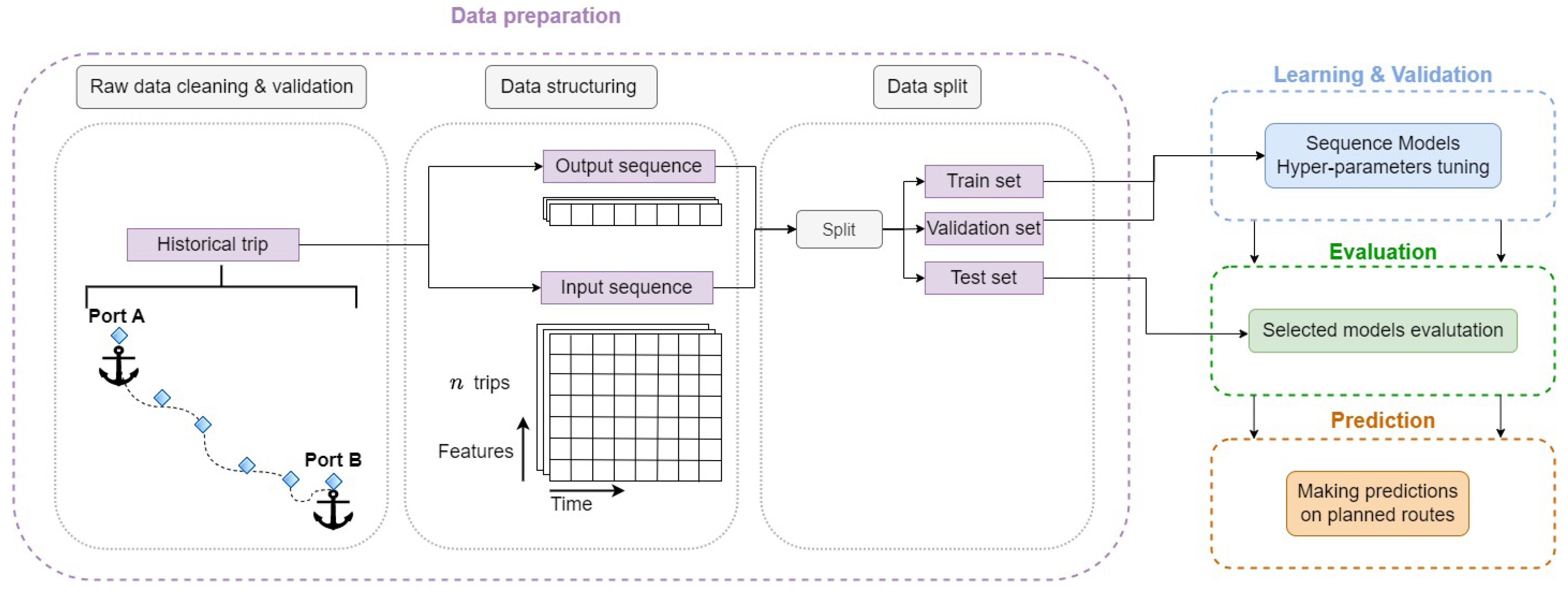
The methodology overview is represented by Figure 2 and shows the four fundamental steps deployed in this study as follows:
  • Data preparation: This step consists of transforming raw data into a suitable form for modeling. This study considers three main preparation operations. The first operation’s objective is to improve the data quality by applying data cleaning and validation techniques. The second operation structures data into input and output sequences for each ship trip. The last operation splits the input and output sequences into training, validation, and test sets. The details of the different operations are provided in Section 3.2
  • Learning and Validation: In the learning phase, the sequence models are trained using the training dataset, composed of input sequences, and the corresponding output sequences to predict the ship speed values that are close to the actual outputs. Hyperparameter optimization is performed according to a validation dataset. The configuration of hyperparameters providing the lowest validation error is selected.
  • Evaluation: The selected models are evaluated using an unseen test dataset for a neutral assessment of their performance. The model with the lowest test error should be selected for the prediction step.
  • Prediction: The best model represents the final solution and can be used to provide ship speed predictions on planned ship trips.

3.2. Data Description and Preparation

This study is based on three years of historical data, spanning the period from January 2019 to December 2020, on ship trips in the area of the Saint Lawrence Seaway from the Atlantic to the port of Montreal. The final dataset used for the training and validation of the predictive models includes 83,993 data points. A data point is a vector composed of the following features:
  • Trip identification number.
  • Ship’s current position latitude (Degrees).
  • Ship’s current position longitude (Degrees).
  • Ship’s next position latitude (Degrees).
  • Ship’s next position longitude (Degrees).
  • Distance between the ship’s current and the following positions (NM).
  • Max draft (Meters).
  • Length overall (Meters).
  • Beam (Meters).
  • Deadweight (Tons).
  • Net tonnage (Tons).
  • Gross tonnage (Tons).
  • Max power (Kilowatts).
  • Age (Years).
  • Vessel type.
The “vessel type” feature is categorical and includes 26 different types of merchant vessels (tankers, bulkers, containerships, etc.), barges, and tug boats.
While many opportunities arise from using real-world data, many challenges also emerge. The data employed in this study are drawn from human and sensor records and, therefore, they have quality issues such as erroneous entries, incomplete values, and outliers. The initial dataset was composed of 190,839 data points. The following cleaning and validation operations were carried out to improve the data quality:
  • Remove duplicate trips.
  • Remove trips with outlier values. A plot of the positions can highlight some position outliers, such as the example in Table 1, which shows two unlikely consecutive points in a trip. The descriptive statistics also indicate the presence of noisy values in the dataset in the distance, travel time, and baseline speed between two consecutive positions. A filtering strategy based on domain knowledge was established to remove trips containing outliers.
  • Impute missing values in vessel particulars using mean values: length, width, deadweight, net tonnage, gross tonnage, max power, and vessel age.
  • Transform the categorical data of “vessel types” into numeric representations using one-hot encoding.
For each point in a trip, the label is the average speed to reach the next point and it is obtained by dividing the distance to the next point by the travel time provided by the difference between the timestamps. The dataset is organized as a collection of ship trips, each formed by a sequence of input data points and the corresponding output sequence. The data from 2019 and 2020 are used for training, the validation is performed on data from the first six months of 2021, and the test performance is evaluated using the the second half of 2021.

3.3. Sequence Models

The machine learning task addressed in this study deals with sequential data, which can be modeled using deep learning sequence models. We briefly review the different types of sequence models used in this study.

3.3.1. Recurrent Neural Networks

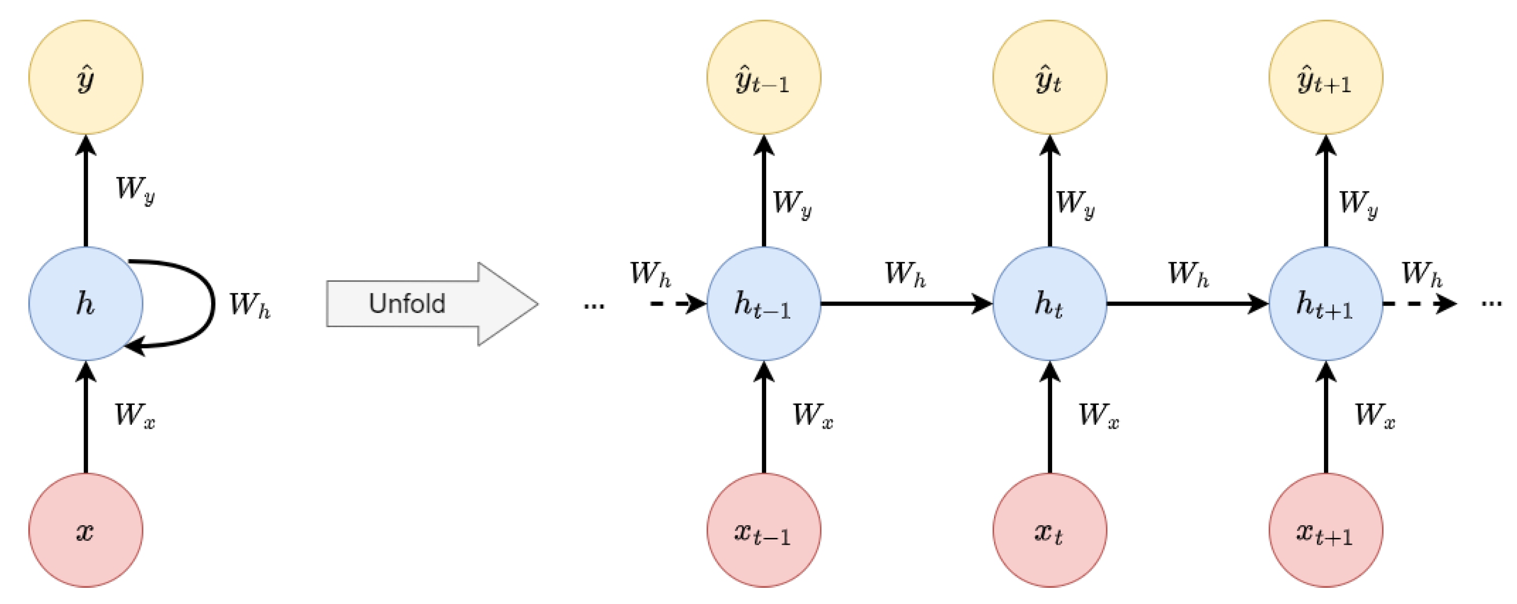
Recurrent Neural Networks (RNNs) are a class of deep learning designed for sequence data; they have been widely used, particularly for natural language text processing. At each step t of the sequence, the RNN performs the same function with the same parameters to predict the value y ^ t using both the current input x t and the previous hidden state h t 1 . This study considers a type of RNN producing an output at each step and having recurrent connections between hidden units, as illustrated by an unfolded representation in Figure 3. The RNN maps an input sequence to an output sequence of the same length. The forward propagation in the RNN is provided by the following Equations (1)–(3). The input to the hidden connections is parameterized by the weight matrix W x , the recurrent connections between hidden units by the weight matrix W h , and the hidden-output connections by the weight matrix W y . The bias vectors are b h and b y . The loss L measures the difference between the RNN’s output y ^ and the true target y of all the time steps.
The activation function σ h of the hidden units is usually the hyperbolic tangent function. As the target y t is continuous and positive, we use a Rectified Linear Unit (ReLU) as the activation function σ y of the output layer. The total loss for a sequence is the sum of the losses over all the time steps and the Back-Propagation Through Time algorithm is used for parameters optimization.
h t = σ h ( W x x t + W h h t 1 + b h )
y ^ t = σ y ( W y h t + b y )
L ( y ^ , y ) = t = 1 T L ( y ^ t , y t )
Learning long-term dependencies is a challenge in RNNs. The propagation of gradients over many stages tends to vanish or explode. Gated RNNs were created to overcome these problems, including the LSTM networks [37], which are better at learning long-term dependencies than normal RNNs. Cells in LSTM networks replace the hidden units of the ordinary RNNs and are connected recurrently to each other. In addition to the input and output of a normal RNN, LSTM networks also have other parameters and a system of gating units to control the information flow. The LSTM cell graph is depicted in Figure 4. LSTM networks use a forget gate f t (4), an input gate i t (5), and an output gate o t (6). A forward pass of an LSTM cell is expressed by the following equations:
f t = σ g ( W f x t + U f h t 1 + b f )
i t = σ g ( W i x t + U i h t 1 + b i )
o t = σ g ( W o x t + U o h t 1 + b o )
c ˜ t = t a n h ( W c ˜ x t + U c ˜ h t 1 + b c ˜ )
c t = f t c t 1 + i t c ˜ t
h t = o t t a n h ( c t )
where σ g is the sigmoid activation function, c ˜ t (7) and c t (8) are the cell states vectors, W and U are weight matrices, b bias vectors, and h t (9) is the output vector of the LSTM layer.
The RNNs discussed so far have a causal structure where the output prediction of a step t depends only on past information. In our application, y ^ t might depend on the whole input sequence. For instance, the average speed needed to reach the next point on the trajectory might depend on the following points in the voyage. This can be addressed using Bidirectional RNNs [38], combining an RNN moving forward and an RNN moving backward. The output at each time step depends on the hidden units of both RNNs accounting for past and future information in the ship trip.

3.3.2. Transformers

The encoder–decoder sequence-to-sequence architecture was proposed to enable an RNN to map an input sequence to an output sequence of different lengths. This architecture is based on an encoder RNN to process the input sequence and a decoder RNN to generate the output sequence. The attention mechanism for encoder–decoder models was first proposed by [39]. The mechanism focuses on particular elements of the input sequence to produce an output at each time step. Transformers [40] are an effective encoder–decoder model based on attention mechanisms without any convolutional or recurrent layers. Transformers have become popular thanks to their ability to handle long sequences using less memory and computational requirements than RNNs. Transformers were initially proposed for text data, but they have been effective in many applications, including vision and speech [41]. The transformer model depicted in Figure 5 has an encoder block preceded by an input layer and a positional encoding layer. The input layer is a fully connected feed-forward network that transforms the input sequence to have d m o d e l features per step. The transformed input sequence is added with positional encoding and fed into the encoder. The encoder block is a stack of l identical encoder layers, each with two sub-layers of multi-head self-attention and position-wise feed-forward networks. The single attention mechanism in the transformer (10) is based on computing the dot product of the query Q with all keys K, dividing by d k , and applying the s o f t m a x function to obtain the weights on the values V:
A t t e n t i o n ( Q , K , V ) = s o f t m a x ( Q K T d k ) V
where d k is the queries and keys dimension.
The multi-head self-attention mechanism consists of linearly projecting the queries, keys, and values h times, with different learnable projections. The single attention mechanism is then performed on each projection, in which the outputs are concatenated and projected again to obtain the final value. Both sub-layers of the encoder use residual connections and are followed by a normalization layer. The output of the encoder is a vector representation of dimension d m o d e l for each position in the input sequence. The encoder output is fed into a feed-forward layer with ReLU activation to produce the output prediction sequence.

4. Experiment

4.1. Experimental Setting and Hyperparameters Optimization

We compare the sequence models of LSTM, BiLSTM, and Transformer networks with the baseline fixed speed rate. The models are implemented using the machine learning library Pytorch [42] and trained on an Nvidia Tesla T4 GPU. The experimental tracking and hyperparameter optimization are performed using the Weights & Biases platform [43]. The implementation templates are available here https://github.com/saraelmekkaoui/seq-models (accessed on 15 October 2022).
The training of the models is performed using the L1-norm loss function (11) and Adam optimizer [44]. The performances of the models are evaluated using the Mean Absolute Error (MAE) (12) and the Mean Squared Error (MSE) (13). The MAE indicates the mean overall observations of the absolute errors between the observations y i and the predictions y ^ i . The MSE expresses the mean of the squared errors vector to the number of samples. In the regression setting, the lower the MAE and MSE values, the higher the model’s accuracy.
L = i = 1 n | y i y ^ i |
M A E = 1 n i = 1 n | y i y ^ i |
M S E = 1 n i = 1 n ( y i y ^ i ) 2
When building machine learning models, the challenge is in finding a model with an appropriate capacity for the task’s complexity and the available training data [45]. The objective is to find a generalizable machine learning model that performs well on training and unseen data. This model should not be overfitting, meaning it has a significant gap between the training data and test data performances. It should also not be underfitting, meaning it has a significant error in the training data. To control the model’s ability for overfitting or underfitting, we alter its capacity, i.e., its ability to fit a wide variety of functions using the hyperparameters. In the case of deep learning models, these hyperparameters can be, for instance, the number of hidden layers, the number of neurons per layer, and the learning rate.
Deep learning models are prone to overfitting because they learn a vast number of parameters to build the model. They are parametric methods, which means they have parameters controlling their behavior. They learn the parameters that minimize the training error using the training data. In order to tune the hyperparameters that control the model’s capacity, we use a validation dataset to estimate the generalization error. The test set is a separate dataset from the training and validation data to evaluate the performance of the model on unseen data. Fitting a deep learning model is time-consuming, as we have many hyperparameters to optimize. The training of the model as well can become longer as we augment the model’s capacity. In order to avoid overfitting, we apply the regularization techniques of dropout, early stopping, and L1 weight decay. Hyperparameters optimization is performed using a random search [46] and the maximum number of iterations is 500. Table 2 reports the values and marginal distributions for all the model-tuned hyperparameters.

4.2. Results and Discussion

For each network type, we train 120 different random configurations of hyperparameters and choose the models with the lowest validation error. The errors between the models’ predictions and targets are measured using the MAE and MSE. The Monte Carlo Dropout technique [47] is used to estimate the uncertainty by considering 50 experimental runs per model and the mean and standard deviation of the MAEs and MSEs over the experiments are reported in Table 3. The comparison of the three sequence models’ predictive accuracy with the baseline speed rates shows the effectiveness of machine learning-based methods in addressing the problem of ship speed prediction.
The results show that the BiLSTM and Transformer models, which account for the information along the ship trip to estimate the ship speed at a particular point, are more accurate than the LSTM model, which considers only the past information from the sequence data to produce a prediction at each point. It also appears that for the Transformer model to be efficient, it needs to be deeper than the corresponding LSTM-based architectures. The importance of hyperparameters with respect to the validation error is depicted in Figure 6. This suggests the hyperparameters to consider for a further tuning of the models. Considering the accuracy, the Transformer model seems to be a promising solution that could be further investigated. The results of this study demonstrate the potential of deep learning models to provide a closer estimate of ship speed to the actual values. The proposed model’s performance, however, should be improved by considering more training data, other inputs such as weather information, or a different modeling perspective to consider the spatial interactions of ships.

4.3. Practical Implications

An accurate estimation of ships’ speeds can improve maritime transport performance, causing it to be more efficient and competitive. First, the prediction of ship speed can improve maritime and logistics stakeholders’ operational and commercial performances. Predicting ships’ speeds can provide reliable ship arrival times to destinations that are not aligned with the efficient planning and scheduling of maritime operations. The benefits could be to shorten vessels’ turnaround times, reduce ship and inland transportation congestion, optimize equipment and resource utilization, and improve inventory management. Supply chain management can also be positively impacted by improving the visibility of the supply chain and the reliability of information transmitted to customers. This can contribute to facilitating the adoption of best practices between the various actors for the better management of cargo flows. The commercial performance of the maritime actors can therefore be enhanced by increasing communication transparency and providing accurate information to clients.
Another promising aspect of ship speed prediction is improving navigation security and safety. An accurate estimation of ship speed can allow for the rigorous monitoring of ships’ movements and support the VTS and concerned authorities’ role to supervise traffic better and prevent possible accidents. It can also help in detecting abnormal ship behavior for security reasons. Ship speed prediction can also help with collision risk assessment. Predicting when ships will arrive at specific points can determine the risk indicators of collision.
Finally, from an environmental perspective, improving port operations, maritime navigation, and supply chain management through the accurate prediction of ship speed could reduce ship emissions. Indeed, the reliable planning of ship routes and port and logistics operations could facilitate the adoption of the “virtual arrival” or “just-in-time” policy. This policy is based on the idea of adjusting a ship’s speed to arrive at its destination at a specified time when the berth is available. As a result, ships can optimize their speed and fuel consumption, thereby reducing emissions [48]. The virtual arrival policy also has other benefits, such as lowering ship waiting times, port congestion, and pollution near ports. In a trial [49], this practice reduced a ship’s fuel consumption by 23% during a particular voyage.

5. Conclusions

Maritime transport is a complex system in which many actors interact to achieve global supply chain connectivity. Given the economic and environmental impact of the maritime industry, digitization is a way of addressing the sector’s challenges and enhancing its performance. Therefore, machine learning methods can extract insights from maritime data to support the sector’s compliance with the regulations and to maintain sustainable growth.
The aim of this study is to build a predictive model for ship speed estimation based on historical ship trip data provided by the VTS for a specific area. The challenge is to produce a predictive model to accommodate different ship types navigating between different origins and destinations. This challenge is addressed using deep learning sequence models to deal with the sequential nature of ship trip data. The problem is formulated as a regression task to predict the value of the speed rate needed at each step in a ship trip to reach the following one. The results show that the proposed models outperform the usual baseline speed rate used by VTS. This work’s outcome could improve the area’s planning and scheduling of maritime operations. This work could enhance maritime transport performance in several ways, including ameliorating the logistics operations efficiency and supply chain performance, ensuring navigation safety and security, and reducing ship emissions.
Although the proposed predictive models are more accurate than usual practice, their performance should be further improved for an effective application. It is also worth highlighting that hyperparameter optimization in deep learning models is among the most critical tasks. The hyperparameters control both the training performance of the model and the quality of the test results. This study considered a random search to determine the best configuration. Other methods could be investigated, such as the Taguchi method [50,51] or the Teaching–Learning-Based Optimization technique [52,53]. Another challenge concerns the lack of interpretability of deep learning models. Future research to improve models’ performances will investigate the effects of weather data integration, data augmentation, and other deep learning model types to capture the spatiotemporal information of ship movements. In addition, further research regarding the interpretation of sequence models should be performed to enhance the reliability of models in managing the risks related to shipping activity.

Author Contributions

Conceptualization, S.E.M. and L.B.; Formal analysis, S.E.M.; Methodology, S.E.M., L.B. and A.B.; Resources, S.C.; Supervision, L.B. and A.B.; Validation, L.B., S.C. and A.B.; Writing—original draft, S.E.M.; Writing—review and editing, S.E.M. All authors have read and agreed to the published version of the manuscript.

Funding

This research received no external funding.

Institutional Review Board Statement

Not applicable.

Informed Consent Statement

Not applicable.

Data Availability Statement

Data sharing is not applicable.

Conflicts of Interest

The authors declare no conflict of interest.

References

  1. Heilig, L.; Stahlbock, R.; Voß, S. From Digitalization to Data-Driven Decision Making in Container Terminals. In Handbook of Terminal Planning; Böse, J.W., Ed.; Springer International Publishing: Cham, Switzerland, 2020; pp. 125–154. [Google Scholar] [CrossRef]
  2. Heilig, L.; Voß, S. Information Systems in Seaports: A Categorization and Overview. Inf. Technol. Manag. 2017, 18, 179–201. [Google Scholar] [CrossRef]
  3. Christiansen, M.; Fagerholt, K.; Nygreen, B.; Ronen, D. Maritime Transportation. In Handbooks in Operations Research and Management Science; Barnhart, C., Laporte, G., Eds.; Elsevier: Amsterdam, The Netherlands, 2007; Volume 14, pp. 189–284. [Google Scholar] [CrossRef]
  4. Prpić-Oršić, J.; Vettor, R.; Faltinsen, O.M.; Guedes Soares, C. The Influence of Route Choice and Operating Conditions on Fuel Consumption and CO2 Emission of Ships. J. Mar. Sci. Technol. 2016, 21, 434–457. [Google Scholar] [CrossRef] [Green Version]
  5. Wang, K.; Yan, X.; Yuan, Y.; Li, F. Real-time Optimization of Ship Energy Efficiency based on the Prediction Technology of Working Condition. Transp. Res. D Transp. 2016, 46, 81–93. [Google Scholar] [CrossRef]
  6. ClearSeas. Navigating the St. Lawrence: Challenging Waters, Rich History and Bright Future. 2020. Available online: https://clearseas.org/en/blog/navigating-the-st-lawrence-challenging-waters-rich-history-and-bright-future/ (accessed on 15 October 2022).
  7. Nguyen, D.D.; Le Van, C.; Ali, M.I. Vessel Trajectory Prediction Using Sequence-to-Sequence Models over Spatial Grid. In Proceedings of the 12th ACM International Conference on Distributed and Event-Based Systems, Hamilton, New Zealand, 25–29 June 2018; Association for Computing Machinery: New York, NY, USA, 2018; pp. 258–261. [Google Scholar] [CrossRef]
  8. Forti, N.; Millefiori, L.M.; Braca, P.; Willett, P. Prediction of Vessel Trajectories From AIS Data Via Sequence-To-Sequence Recurrent Neural Networks. In Proceedings of the ICASSP 2020—2020 IEEE International Conference on Acoustics, Speech and Signal Processing (ICASSP), Barcelona, Spain, 4–8 May 2020; pp. 8936–8940. [Google Scholar] [CrossRef]
  9. Suo, Y.; Chen, W.; Claramunt, C.; Yang, S. A Ship Trajectory Prediction Framework Based on a Recurrent Neural Network. Sensors 2020, 20, 5133. [Google Scholar] [CrossRef]
  10. You, L.; Xiao, S.; Peng, Q.; Claramunt, C.; Han, X.; Guan, Z.; Zhang, J. ST-Seq2Seq: A Spatio-Temporal Feature-Optimized Seq2Seq Model for Short-Term Vessel Trajectory Prediction. IEEE Access 2020, 8, 218565–218574. [Google Scholar] [CrossRef]
  11. Capobianco, S.; Millefiori, L.M.; Forti, N.; Braca, P.; Willett, P. Deep Learning Methods for Vessel Trajectory Prediction Based on Recurrent Neural Networks. IEEE Aerosp. Electron. Syst. 2021, 57, 4329–4346. [Google Scholar] [CrossRef]
  12. El Mekkaoui, S.; Benabbou, L.; Berrado, A. Deep Learning Models for Vessel’s ETA Prediction: Bulk Ports Perspective. Flex. Serv. Manuf. 2022, 1–24. [Google Scholar] [CrossRef]
  13. Yan, R.; Wang, S.; Zhen, L.; Laporte, G. Emerging Approaches Applied to Maritime Transport Research: Past and Future. Commun. Transp. Res. 2021, 1, 100011. [Google Scholar] [CrossRef]
  14. Tu, E.; Zhang, G.; Rachmawati, L.; Rajabally, E.; Huang, G.B. Exploiting AIS Data for Intelligent Maritime Navigation: A Comprehensive Survey From Data to Methodology. IEEE Trans. Intell. Transp. Syst. 2018, 19, 1559–1582. [Google Scholar] [CrossRef]
  15. Alessandrini, A.; Mazzarella, F.; Vespe, M. Estimated Time of Arrival Using Historical Vessel Tracking Data. IEEE Trans. Intell. Transp. Syst. 2019, 20, 7–15. [Google Scholar] [CrossRef]
  16. Öztürk, Ü.; Akdağ, M.; Ayabakan, T. A Review of Path Planning Algorithms in Maritime Autonomous Surface Ships: Navigation Safety Perspective. Ocean Eng. 2022, 251, 111010. [Google Scholar] [CrossRef]
  17. Sharma, K.; Swarup, C.; Pandey, S.K.; Kumar, A.; Doriya, R.; Singh, K.; Singh, T. Early Detection of Obstacle to Optimize the Robot Path Planning. Drones 2022, 6, 265. [Google Scholar] [CrossRef]
  18. Hoffmann Pham, K.; Boy, J.; Luengo-Oroz, M. Data Fusion to Describe and Quantify Search and Rescue Operations in the Mediterranean Sea. In Proceedings of the 2018 IEEE 5th International Conference on Data Science and Advanced Analytics (DSAA), Turin, Italy, 1–3 October 2018; pp. 514–523. [Google Scholar] [CrossRef]
  19. Sharma, K.; Doriya, R.; Pandey, S.K.; Kumar, A.; Sinha, G.R.; Dadheech, P. Real-Time Survivor Detection System in SaR Missions Using Robots. Drones 2022, 6, 219. [Google Scholar] [CrossRef]
  20. Harati-Mokhtari, A.; Wall, A.; Brooks, P.; Wang, J. Automatic Identification System (AIS): Data Reliability and Human Error Implications. J. Navig. 2007, 60, 373–389. [Google Scholar] [CrossRef]
  21. Masnicki, R.; Mindykowski, J. Case Study—Based ZigBee Network Implementation for Maritime On-Board Safety Improvement. In Proceedings of the 2019 IMEKO TC-19 International Workshop on Metrology for the Sea, Genova, Italy, 3–5 October 2019; pp. 3–5. [Google Scholar]
  22. AlShuhail, A.S.; Bhatia, S.; Kumar, A.; Bhushan, B. Zigbee-Based Low Power Consumption Wearables Device for Voice Data Transmission. Sustainability 2022, 14, 10847. [Google Scholar] [CrossRef]
  23. Zhang, S.; Wu, R.; Xu, K.; Wang, J.; Sun, W. R-CNN-Based Ship Detection from High Resolution Remote Sensing Imagery. Remote Sens. 2019, 11, 631. [Google Scholar] [CrossRef] [Green Version]
  24. Rostami, M.; Kolouri, S.; Eaton, E.; Kim, K. Deep Transfer Learning for Few-Shot SAR Image Classification. Remote Sens. 2019, 11, 1374. [Google Scholar] [CrossRef] [Green Version]
  25. Zhang, Y.; Guo, L.; Wang, Z.; Yu, Y.; Liu, X.; Xu, F. Intelligent Ship Detection in Remote Sensing Images Based on Multi-Layer Convolutional Feature Fusion. Remote Sens. 2020, 12, 3316. [Google Scholar] [CrossRef]
  26. Wu, Y.; Ma, W.; Gong, M.; Bai, Z.; Zhao, W.; Guo, Q.; Chen, X.; Miao, Q. A Coarse-to-Fine Network for Ship Detection in Optical Remote Sensing Images. Remote Sens. 2020, 12, 246. [Google Scholar] [CrossRef] [Green Version]
  27. Li, L.; Zhou, Z.; Wang, B.; Miao, L.; An, Z.; Xiao, X. Domain Adaptive Ship Detection in Optical Remote Sensing Images. Remote Sens. 2021, 13, 3168. [Google Scholar] [CrossRef]
  28. Mao, W.; Rychlik, I.; Wallin, J.; Storhaug, G. Statistical Models for the Speed Prediction of a Container Ship. Ocean Eng. 2016, 126, 152–162. [Google Scholar] [CrossRef]
  29. Li, G.; Kawan, B.; Wang, H.; Zhang, H. Neural-Network-based Modelling and Analysis for Time Series Prediction of Ship Motion. Ship Technol. Res. 2017, 64, 30–39. [Google Scholar] [CrossRef] [Green Version]
  30. Gan, S.; Liang, S.; Li, K.; Deng, J.; Cheng, T. Long-Term Ship Speed Prediction for Intelligent Traffic Signaling. IEEE Trans. Intell. Transp. Syst. 2017, 18, 82–91. [Google Scholar] [CrossRef]
  31. Abebe, M.; Shin, Y.; Noh, Y.; Lee, S.; Lee, I. Machine Learning Approaches for Ship Speed Prediction towards Energy Efficient Shipping. Appl. Sci. 2020, 10, 2325. [Google Scholar] [CrossRef] [Green Version]
  32. Krata, P.; Vettor, R.; Soares, C.G. Bayesian Approach to Ship Speed Prediction based on Operational Data. In Developments in the Collision and Grounding of Ships and Offshore Structures; Taylor & Francis Group: London, UK, 2020; pp. 384–390. [Google Scholar]
  33. Moreira, L.; Vettor, R.; Guedes Soares, C. Neural Network Approach for Predicting Ship Speed and Fuel Consumption. J. Mar. Sci. Eng. 2021, 9, 119. [Google Scholar] [CrossRef]
  34. Baier, A.; Boukhers, Z.; Staab, S. Hybrid Physics and Deep Learning Model for Interpretable Vehicle State Prediction. arXiv 2021, arXiv:abs/2103.06727. [Google Scholar]
  35. Yoo, B.; Kim, J. Probabilistic Modeling of Ship Powering Performance using Full-Scale Operational Data. Appl. Ocean Res. 2019, 82, 1–9. [Google Scholar] [CrossRef]
  36. IMO. Vessel Traffic Services. 2019. Available online: https://www.imo.org/en/OurWork/Safety/Pages/VesselTrafficServices.aspx (accessed on 16 October 2022).
  37. Hochreiter, S.; Schmidhuber, J. Long Short-Term Memory. Neural Comput. 1997, 9, 1735–1780. [Google Scholar] [CrossRef]
  38. Schuster, M.; Paliwal, K. Bidirectional Recurrent Neural Networks. IEEE Trans. Signal. Inf. Process. 1997, 45, 2673–2681. [Google Scholar] [CrossRef] [Green Version]
  39. Bahdanau, D.; Cho, K.; Bengio, Y. Neural Machine Translation by Jointly Learning to Align and Translate. In Proceedings of the 3rd International Conference on Learning Representations, ICLR 2015, San Diego, CA, USA, 7–9 May 2015. [Google Scholar]
  40. Vaswani, A.; Shazeer, N.; Parmar, N.; Uszkoreit, J.; Jones, L.; Gomez, A.N.; Kaiser, L.; Polosukhin, I. Attention is All you Need. In Proceedings of the Advances in Neural Information Processing Systems, Long Beach, CA, USA, 4–9 December 2017. [Google Scholar]
  41. Lin, T.; Wang, Y.; Liu, X.; Qiu, X. A Survey of Transformers. AI Open 2022, 3, 111–132. [Google Scholar] [CrossRef]
  42. Paszke, A.; Gross, S.; Massa, F.; Lerer, A.; Bradbury, J.; Chanan, G.; Killeen, T.; Lin, Z.; Gimelshein, N.; Antiga, L.; et al. PyTorch: An Imperative Style, High-Performance Deep Learning Library. In Proceedings of the Advances in Neural Information Processing Systems, Vancouver, BC, Canada, 8–14 December 2019. [Google Scholar]
  43. Biewald, L. Experiment Tracking with Weights and Biases. Available online: https://www.wandb.com/ (accessed on 9 October 2022).
  44. Kingma, D.P.; Ba, J. Adam: A Method for Stochastic Optimization. In Proceedings of the 3rd International Conference on Learning Representations, ICLR 2015, San Diego, CA, USA, 7–9 May 2015. [Google Scholar]
  45. Goodfellow, I.; Bengio, Y.; Courville, A. Deep Learning; MIT Press: Cambridge, MA, USA, 2016; Available online: http://www.deeplearningbook.org (accessed on 27 September 2022).
  46. Bergstra, J.; Bengio, Y. Random Search for Hyper-Parameter Optimization. J. Mach. Learn. Res. 2012, 13, 281–305. [Google Scholar]
  47. Gal, Y.; Ghahramani, Z. Dropout as a Bayesian Approximation: Representing Model Uncertainty in Deep Learning. In Proceedings of the 33rd International Conference on Machine Learning, New York, NY, USA, 20–22 June 2016. [Google Scholar]
  48. PortXchange. How Just-In-Time Arrivals Can Reduce Shipping Emissions. 2022. Available online: https://port-xchange.com/blog/just-in-time-arrivals-cutting-emissions-today/ (accessed on 26 October 2022).
  49. IMO. Desktop Just-In-Time Trial Yields Positive Results in Cutting Emissions. 2019. Available online: https://www.imo.org/en/MediaCentre/Pages/WhatsNew-1326.aspx (accessed on 11 October 2022).
  50. Rahman, M.A.; chandren Muniyandi, R.; Albashish, D.; Rahman, M.M.; Usman, O.L. Artificial Neural Network with Taguchi Nethod for Robust Classification Model to Improve Classification Accuracy of Breast Cancer. PeerJ Comput. Sci. 2021, 7, e344. [Google Scholar] [CrossRef] [PubMed]
  51. Huynh, N.T.; Nguyen, T.V.T.; Nguyen, Q.M. Optimum Design for the Magnification Mechanisms Employing Fuzzy Logic–ANFIS. Comput. Mater. Contin 2022, 73, 5961–5983. [Google Scholar] [CrossRef]
  52. Ang, K.M.; El-kenawy, E.S.M.; Abdelhamid, A.A.; Ibrahim, A.; Alharbi, A.H.; Khafaga, D.S.; Tiang, S.S.; Lim, W.H. Optimal Design of Convolutional Neural Network Architectures Using Teaching & Learning-Based Optimization for Image Classification. Symmetry 2022, 14, 2323. [Google Scholar] [CrossRef]
  53. Wang, C.N.; Yang, F.C.; Nguyen, V.T.T.; Vo, N.T.M. CFD Analysis and Optimum Design for a Centrifugal Pump Using an Effectively Artificial Intelligent Algorithm. Micromachines 2022, 13, 1208. [Google Scholar] [CrossRef]
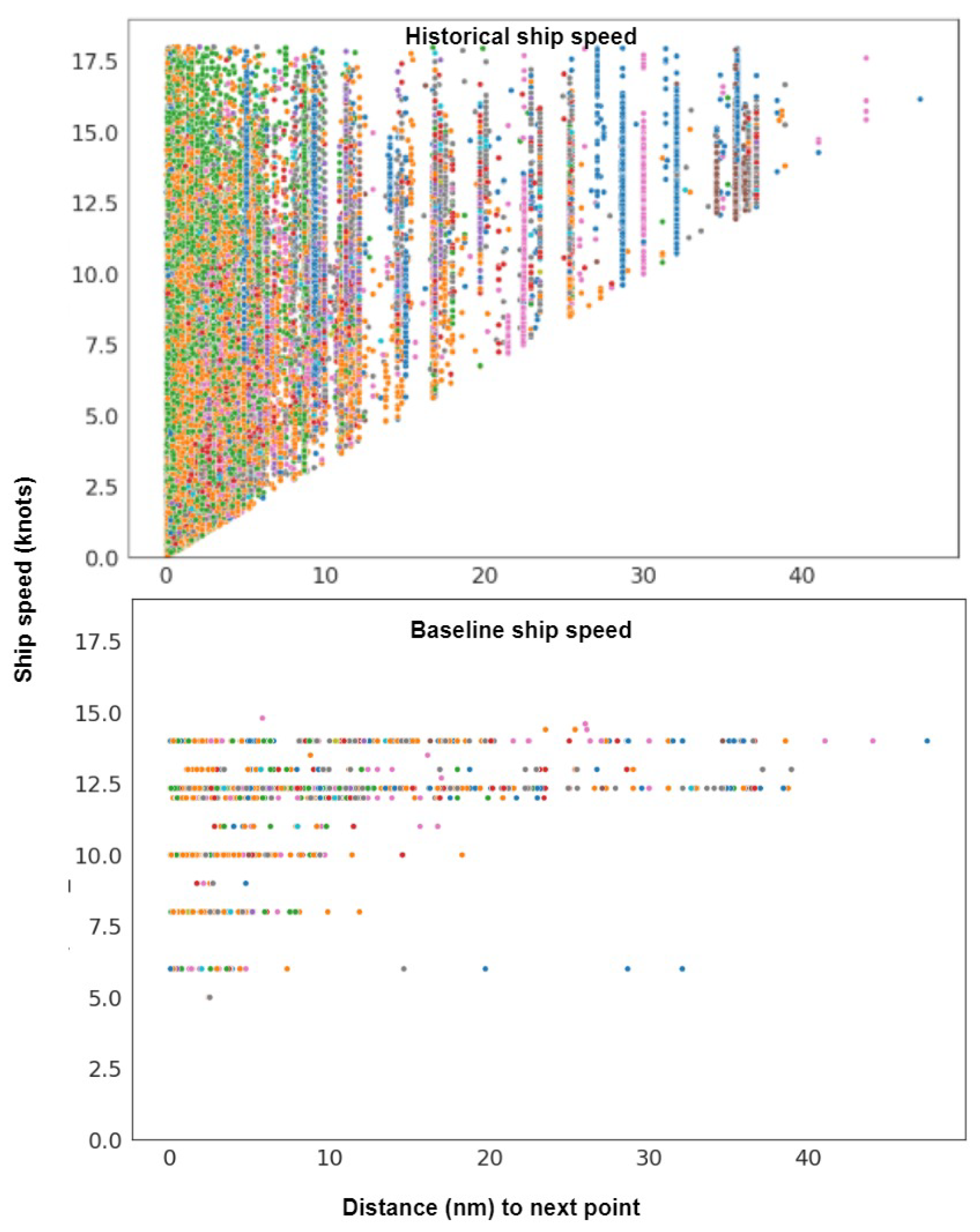
Figure 1. Visualization of the baseline speed and the actual speed per distance between two consecutive trajectory points.
Jmse 11 00191 g001
Figure 2. Overview of the methodology for ship speed prediction.
Jmse 11 00191 g002
Figure 3. A representation of Recurrent Neural Networks.
Jmse 11 00191 g003
Figure 4. A representation of the LSTM cell.
Jmse 11 00191 g004
Figure 5. The architecture of the Transformer model.
Jmse 11 00191 g005
Figure 6. Hyperparameters importance with respect to the validation error.
Jmse 11 00191 g006
Table 1. An example of a position outlier.
Timestamp (UTC)Position Latitude (Degrees)Position Longitude (Degrees)Distance (NM)
22 August 2019 18:03:0048.60−62.45487.32
22 August 2019 19:17:0040.89−66.0440.89
Table 2. Hyperparameters search space.
HyperparameterLSTM and Bi-LSTMTransformer
Learning rateUniform distribution on a log scale between −1 and −5Uniform distribution on a log scale between −1 and −5
Weight decayUniform distribution on a log scale between −4 and −2Uniform distribution on a log scale between −4 and −2
Batch size *[64, 128, 256][64, 128, 256]
Layers *[1, 2]-
DimensionIntegers between 32 and 160 with evenly distributed logarithms-
d m o d e l -Integers between 20 and 80 with evenly distributed logarithms
Encoder feed-forward dimension-Integers between 32 and 256 with evenly distributed logarithms
Dropout *-[0.1, 0.2, 0.3, 0.4]
Number of heads *-[2, 4, 6]
Number of layers *-[1, 2, 3, 4, 5]
* Selection with an equal probability between predefined values.
Table 3. Mean Error (knots) on test data of the selected models.
ModelsLSTMBiLSTMTransformerBaseline
MAE2.43 +/− 0.012.12 +/− 0.011.80 +/− 0.0035.58
MSE11.94 +/− 0.109.47 +/− 0.067.99 +/− 0.0346.71
Number of parameters44,33543,841745,842-
Runtime10 m 8 s24 m 9 s42 m 16 s-
Disclaimer/Publisher’s Note: The statements, opinions and data contained in all publications are solely those of the individual author(s) and contributor(s) and not of MDPI and/or the editor(s). MDPI and/or the editor(s) disclaim responsibility for any injury to people or property resulting from any ideas, methods, instructions or products referred to in the content.