Article

Trajectory Planning of USV: On-Line Computation of the Double S Trajectory Based on Multi-Scale A* Algorithm with Reeds–Shepp Curves

Laboratory of Marine Simulation and Control, Dalian Maritime University, Dalian 116026, China
*
Author to whom correspondence should be addressed.
J. Mar. Sci. Eng. 2023, 11(1), 153; https://doi.org/10.3390/jmse11010153
Submission received: 28 November 2022 / Revised: 25 December 2022 / Accepted: 5 January 2023 / Published: 8 January 2023
(This article belongs to the Section Ocean Engineering)

Abstract

:
Trajectory planning aims to provide a time-related control target that contains the concerned states. For an underactuated surface vehicle (USV), planning challenges include limitations on curvature, speed, acceleration, and jerk. These challenges are relevant for the precise control of USVs. To solve these problems, an on-line double S method and multi-scale A* trajectory planning algorithm is proposed by integrating Reeds–Shepp curves (RSC), where a quad-tree-based graph is used for path planning and collision detection. Simulations illustrate that the proposed method has a better performance than the smooth rapid-exploration random tree (smooth-RRT) method and jump point search (JPS) method, and that path length and the state limitations are satisfied.

1. Introduction

The planning of suitable trajectories is a key process in order to avoid undesired effects such as vibrations or even damage to the mechanical structure of USVs. This paper deals with problems related to global trajectories for the actuation system of USVs.
Commonly used planning methods are the line-of-sight (LOS) method [1], dynamic virtual ship (DVS) method [2,3], and coordinate transformation method [4,5]. They deal with local planning to avoid collisions and provide motion guidance. Generally, local planning is based on a pre-designed global path, derived using methods such as A*, RRT*, and ant colony algorithms. Besides finding a path, the satisfaction of constraints including smoothness and other limitations are also important for path or trajectory planning. In [6], an improved A* algorithm was proposed for USVs to solve map resolution constraints and increase the path smoothness. Reference [7] increased the number of neighboring nodes in an A* algorithm so that smoothness was improved. These research papers explored the configuration of the A* algorithm, but their computational load was relatively heavy. More commonly adopted methods are other variants of the A* algorithm such as the Theta* algorithm [8] or JPS algorithm [9]. Their searching speed is much faster. Reference [10] proposes a hybrid A* algorithm, which allows a continuous state association between grids and guarantees the feasibility of path tracking. In [11] and [12], a smooth-RRT* and an ant colony algorithm were used. The two methods introduced random searching in the scheme, which were efficient for general situations, but unsuitable for areas with narrow connections, such as dumbbell-shaped areas.
There are two main factors of concern in global planning: motion constraints and searching speed. Motion constraints of a USV consist mainly of kinodynamic constraints and non-holonomic constraints. In [13], an admissible velocity propagation method was proposed, that enabled path-velocity decomposition to discover truly dynamic motions. In [14], a framework was presented to extend a RRT algorithm to plan the motion of a wheeled robot under kinodynamic constraints. In [15], the double S trajectory planning method was proposed, which guaranteed a smooth change of speed and acceleration. For non-holonomic constraints, Reeds–Shepp curves [16] or Dubins curves [17] are commonly used. By setting a maximum curvature, the whole path meets the holonomic constraints.
As the demand for precision is different in different positions and environments, multi-scale algorithms are widely applied for searching speed improvements. Reference [18] clarified how to build a quad-tree-based multi-scale map. References [19,20] used multi-scale methods to build maps for unmanned aerial vehicles (UAVs) and wheeled robots, respectively. Reference [21] used a multi-scale Theta* algorithm to plan a path across the Singapore Strait for a USV. They all achieved good planning results.
Based on the methods and analysis above, the main contributions of this research are given as follows: (1) a multi-scale planning graph is established through a quad-tree method, resulting in fast searching. (2) Trajectories can be planned with only initial and final states; curvature constraints are satisfied by Reeds–Sheep curves (RSC), and kinodynamic constraints are satisfied by an on-line double S planning method.

2. Establishment of Multi-Scale Graph

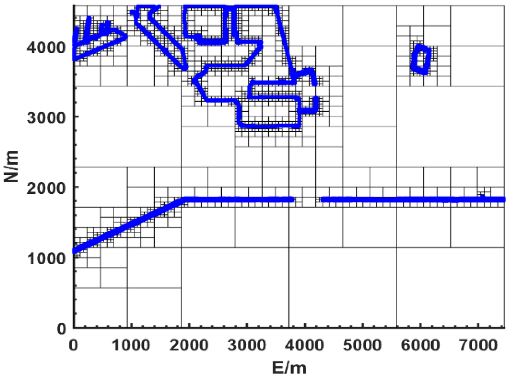
In this research, a quad-tree method is applied to build a graph with finite rectangular regions. The basic idea of the quad-tree is to recursively divide geographic space into different levels of the tree structure. It divides the space of the known range into four equal subspaces, and recurses until the tree reaches a certain depth or does not contain any obstacles. The structure of the quad-tree is simple, and has a high efficiency for spatial data insertion and query. The structure of a regular quad-tree is shown in Figure 1. Geospatial objects are stored on leaf nodes, while internal nodes do not store geospatial objects.
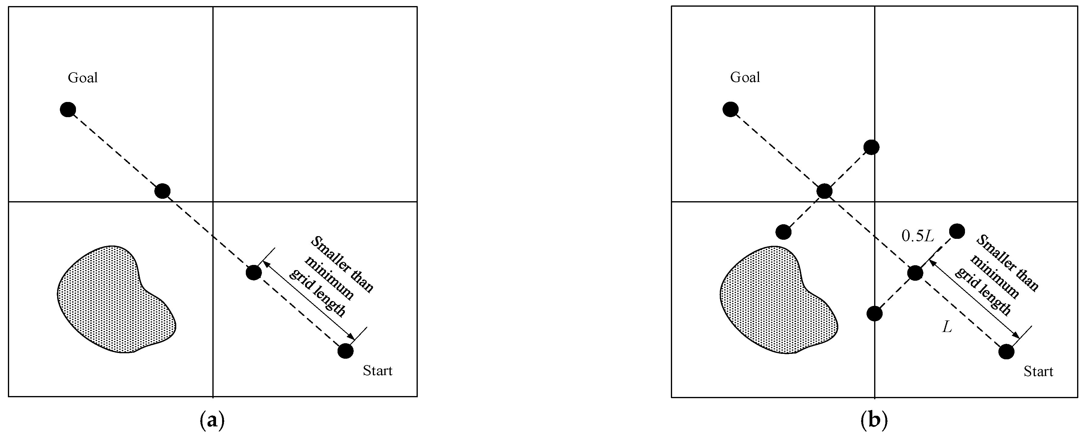
There are several functions that can be achieved through quad-tree. For example, to find which region a point belongs to, the search moves down the tree until it reaches a leaf node, or the lowest level of the tree. This node defines the smallest region in the graph that contains the point. All other points that fall within this region have the same representation in the tree. To find the nodes of neighboring regions of a region on a multi-scale map, a grid of points around the search point can be constructed. After removal of duplicates, the quad-tree regions that contain these points are the neighbors of the initial region. To test for obstacles through the LOS method, sight lines are replaced by a series of points on the line or lines. In practice, generally discretization with small steps on the sight line is enough (Figure 2a). If one needs an assured detection in spite of the possibility of obtaining a longer path, the parallel lines as in Figure 2b should be tested as well. Figure 2 illustrates how the two LOS detection schemes work. If a test point belongs to an obstacle node, this sight line is seen as blocked.
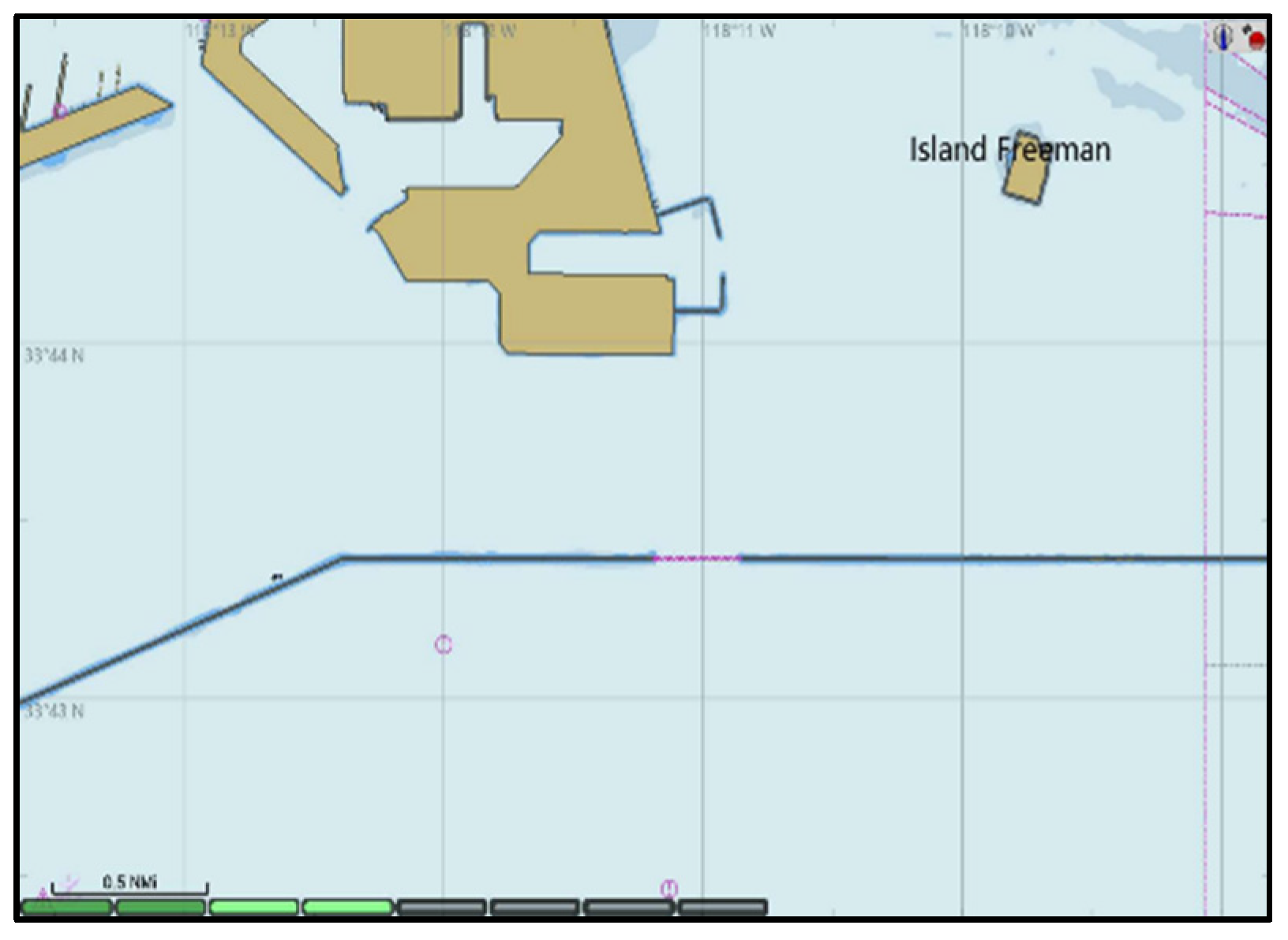
In this research, a part of Long Beach Harbor is taken as the planning environment. The land and obstacles are transferred into points by image processing, so that the quad-tree decomposition can be carried out. Figure 3 is the original navigation chart; Figure 4 is the corresponding multi-scale graph. The nodes containing the colored points are defined as obstacle nodes. Others are traversable nodes. Note, however, that the nodes surrounded by obstacle nodes are untraversable. For this reason, points inside the seashore are not defined as obstacles, to avoid unnecessary calculations.

3. Path Planning Based on Multi-Scale A* Algorithm and RSC

With the established multi-scale graph and neighboring region-searching method, the A* algorithm can be used directly. The implementation of the A* algorithm is given as Algorithm 1, where N is a node, F(N) is the cost of the node, which consists of g(N), the moving cost from start point to node N, and h(N) the heuristic cost.
F ( N )   =   g ( N )   +   h ( N )
Algorithm 1 A* algorithm
1
2
3
4
5
6
7
8
9
10
11
12
13
14
15
16
17
OPEN //the set of nodes to be evaluated
CLOSED //the set of nodes already evaluated
 add the start node to OPEN
 loop
  current=node in OPEN with the lowest cost F(N)
  remove current from OPEN
  add current to CLOSED
  if current is the target node //path has been found
 return
  foreach neighbor of the current node
 if neighbor is not traversable or neighbor is in CLOSED
 skip to the next neighbor
  if new path to neighbor has smaller f_cost or neighbor is not in OPEN
 set f_cost of neighbor
 set parent of neighbor to current
 if neighbor is not in OPEN
 add neighbor to OPEN
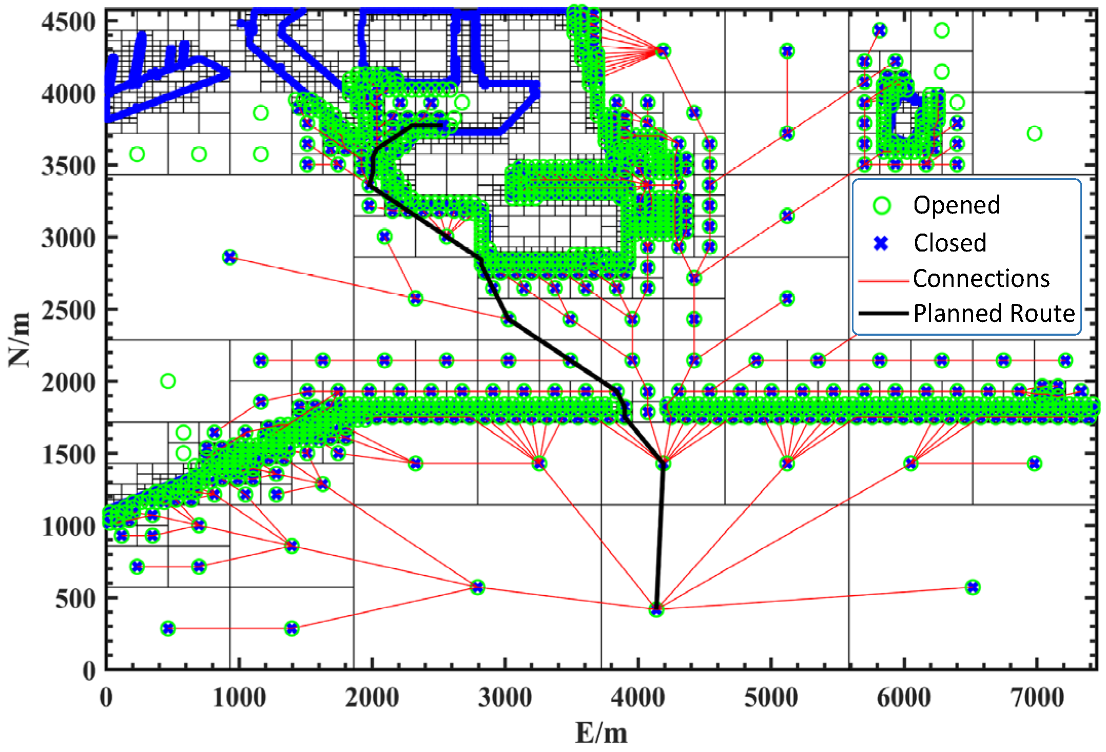
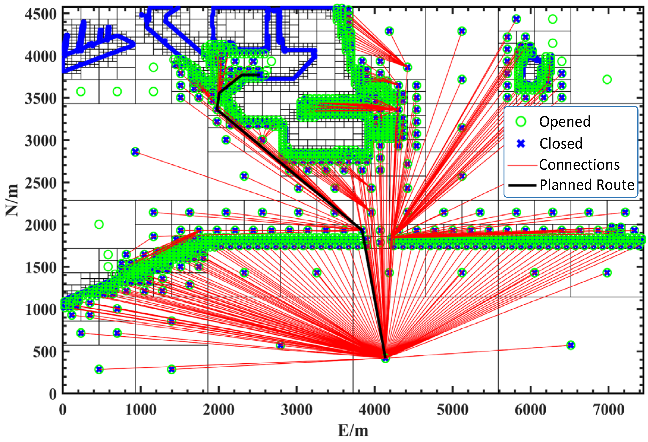
By the direct use of the multi-scale A* algorithm, the node connections and path planning result are shown as Figure 5.
From Figure 5, it can be concluded that the pure A* algorithm causes unnecessary zig-zag paths. This problem may be not that serious in a normal grid-based A* algorithm because it has more nodes than a multi-scale A* algorithm, and the path it produces can easily be corrected with a smoothing algorithm. However, in the multi-scale scheme, some nodes are large in size, meaning that the zig-zags in the path cannot be smoothed easily. To resolve this problem, at each step before checking whether the neighbor of a node is traversable or not by the LOS method in the quad-tree, the parent to the neighbor is checked first. If it is traversable, the parent node of the current node is set as the parent of this neighbor, and corresponding operations are made thereafter. Modifications can be inserted between line 9 and line 10 as:
1
2
3
4
5
6
7
8
 foreach neighbor of the current node
 if neighbor is not traversable from its parent or neighbor is in CLOSED
 skip to the next neighbor
 if new path to neighbor has smaller f_cost or neighbor is not in OPEN
 set f_cost of neighbor
 set parent of neighbor to parent
 if neighbor is not in OPEN
 add neighbor to OPEN
The effect of this modification is shown in Figure 6. Unnecessary zig-zags are avoided after modification.
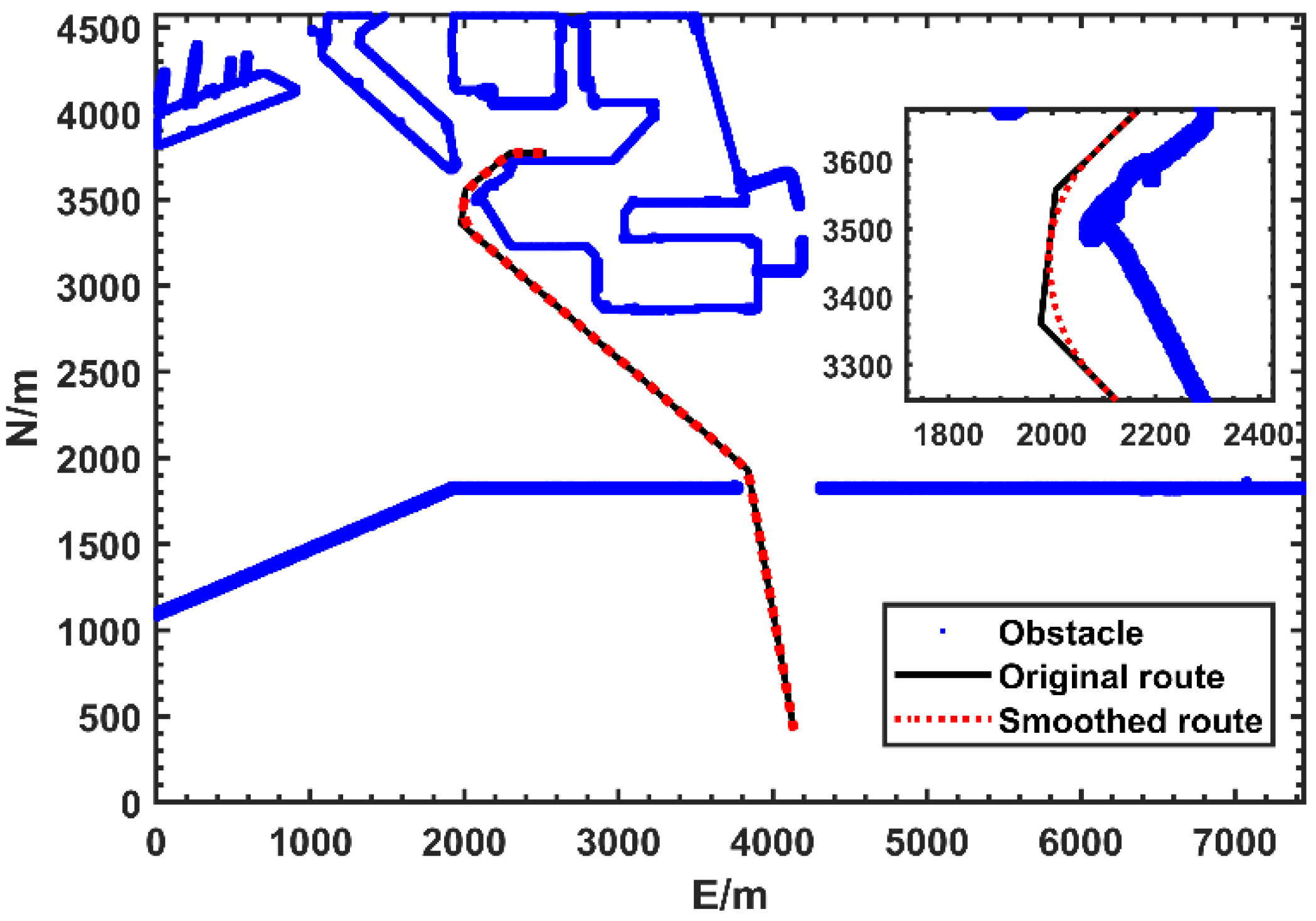
The path under this modified A* algorithm has a much better performance in path length and turnings. Then, the path is smoothed by the G2CBS path-smoothing algorithm [22], as shown in Figure 7. By now, this path can be seen as a satisfactory one for vehicles without non-holonomic constraints. However, for a USV, because the initial and end states are not arbitrary, this path is still not suitable.
RSC [23] refers to the shortest path with, at most, two cusps or reversals, where the direction of the starting point and the end point and the maximum curvature of the path are specified. As long as there is a collision-free path between two nodes, there will be a collision-free RSC between the two nodes. In [10], this method is used to plan the arrival part of the path for a hybrid A* algorithm with impressive results. In light of their thinking, this research applied RSC at the beginning and end parts of the path to facilitate the berthing process. When using this method, penalties should be adjusted from pure distance to weighted distance, so that long backward motions are avoided.
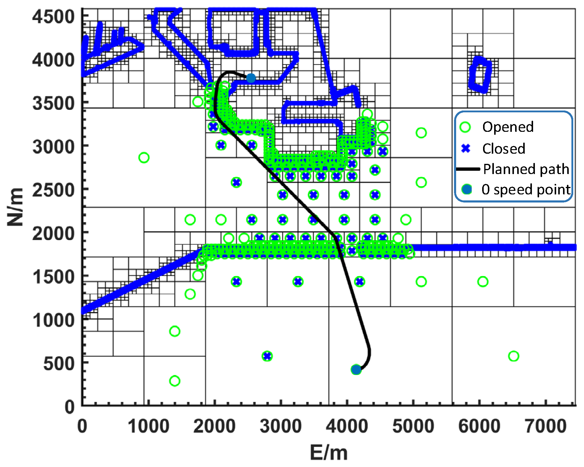
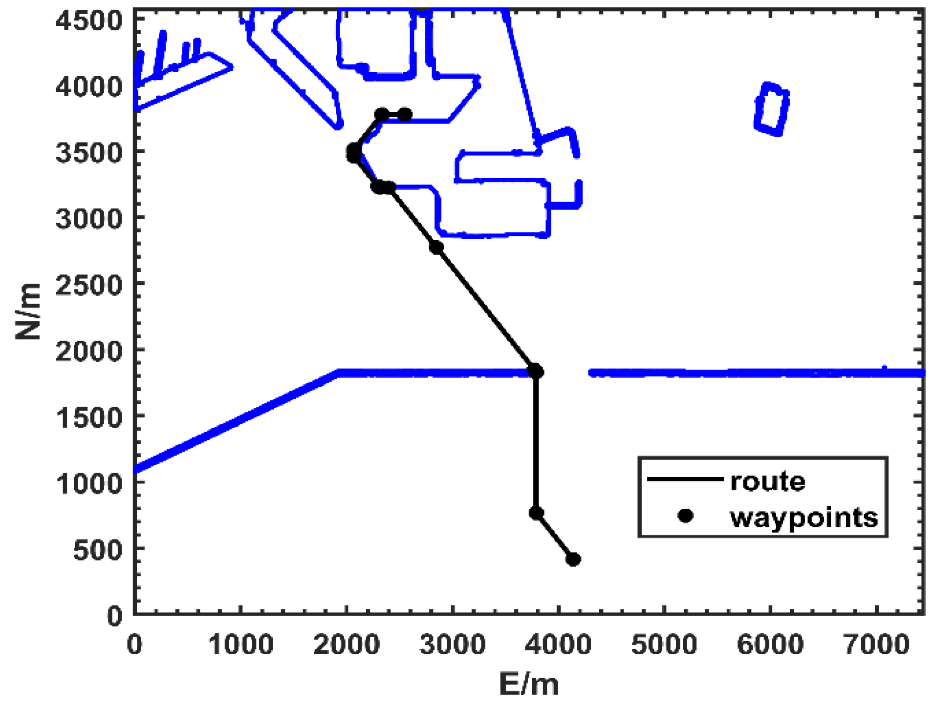
With these methods, and setting the maximum curvature as 0.005, initial pose as [x0, y0, Ψ0] = [4138, 417, 0], and final pose as [x1, y1, Ψ1] = [2548, 3777, 0], the path-planning result is shown in Figure 8. The hollow circles denote nodes that are added once into the open set, and crosses correspond to the closed set. The benefits of the multi-scale method are visible, in that the number of opened nodes is small in spite of the large covered region. Solid circles denote zero-speed points, which are used to denote points where the direction of motion changes in a complex route.
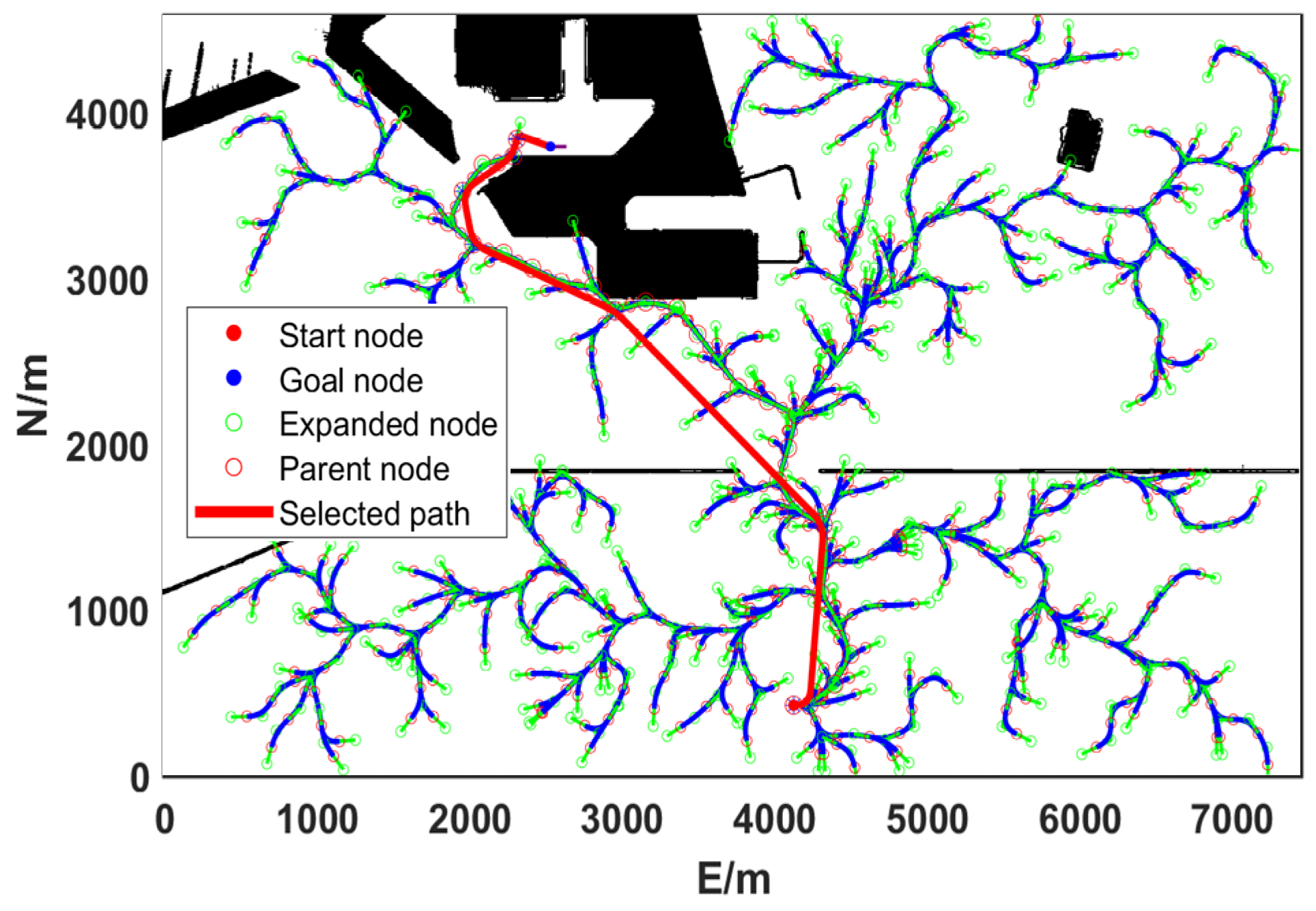
Smooth-RRT and JPS are widely used path-planning methods. Figure 9 and Figure 10 illustrate the plans they generate for the same problem; evaluation metrics are summarized in Table 1 for comparison. The three algorithms were executed using the same devices, so the comparison reflected their complexity. It can be concluded that the proposed method is much faster than smooth-RRT and is close to the speed of JPS (grid size 10 m). JPS is the fastest method, but the constraints are not satisfied. Notably, JPS can only find paths on regular grid maps, and the nodes or edges on the map cannot be weighted. As a result, the path is next to the seashore and increases the risk of collision. Compared to JPS, the route obtained by the proposed method is a bit longer, but it is completely within the safety margin. Expansions are the nodes checked during path planning, and the amount of them directly effects the speed of path planning. Multi-scale A* only uses 12.4% of the nodes used in smooth-RRT. JPS uses 3.8% of the nodes of smooth-RRT, but the constraints are not satisfied.

4. On-Line Computation of the Double S Trajectory

On-line computation of double S trajectories is suitable for paths that include several double S segments, and it is defined in discrete time. At each step the parameters are calculated based on current states, so this trajectory calculation is called on-line. Let
{ q ( t = k T s ) = q k q ˙ ( t = k T s ) = q ˙ k q ¨ ( t = k T s ) = q ¨ k q ( t = k T s ) = q k
denote the values of position, velocity, acceleration, and jerk at the k-th time instant, respectively, and let Ts denote the sampling period. The structure of the trajectory planner is shown in Figure 11. Given the initial and final values of position, velocity, and acceleration and their constraints (vmax, vmin, amax, amin, jmax, jmin), recursion to the next time step is computed as Equation (3). During the planning process, jerk is only selected from three values, jmax, jmin, and 0, to approach all the desired constraints and values.
q ¨ k = q ¨ k 1 + T s 2 ( q k 1 + q k ) q ˙ k = q ˙ k 1 + T s 2 ( q ¨ k 1 + q ¨ k ) q k = q k 1 + T s 2 ( q ˙ k 1 + q ˙ k )
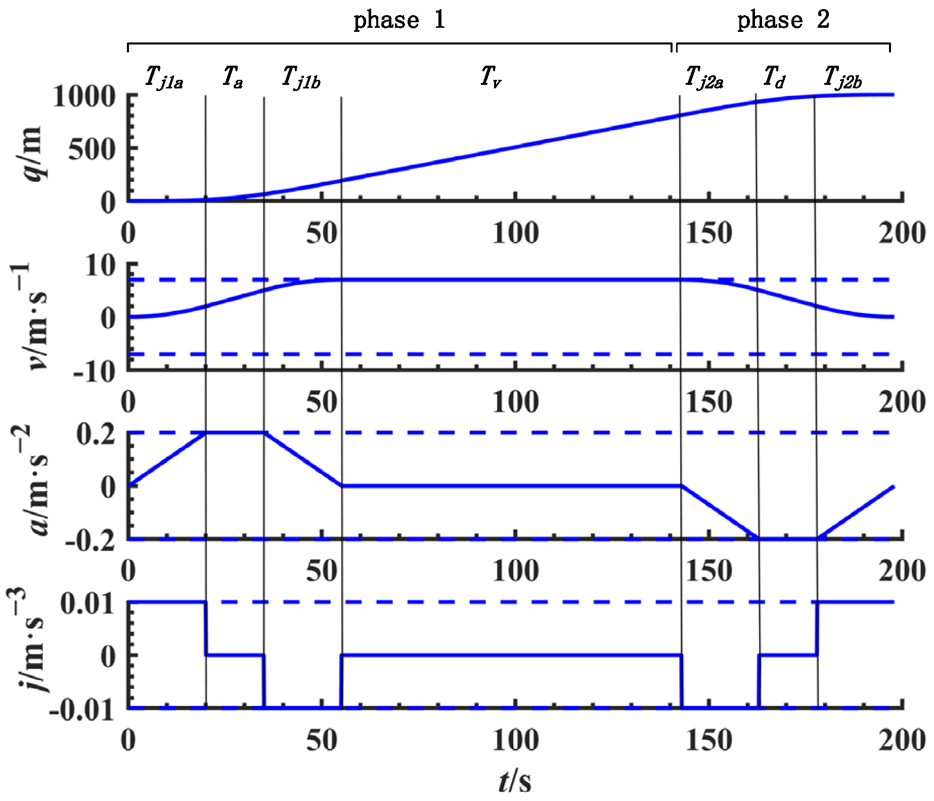
The computation of the trajectory is composed of two phases [15]; Figure 12 is an intuitive illustration of the process.
Phase 1: Acceleration and constant velocity phase
An acceleration profile is computed with the classical trapezoidal acceleration, possibly followed by a constant maximum velocity phase. The jerk is calculated as
q k = { j max ,   if   q ˙ k q ¨ k 2 2 j min < v max and q ¨ k < a max 0 ,   if   q ˙ k q ¨ k 2 2 j min < v max and q ¨ k a max j min ,   if   q ˙ k q ¨ k 2 2 j min v max and q ¨ k > 0 0 ,   if   q ˙ k q ¨ k 2 2 j min v max and q ¨ k 0
Phase 2: Deceleration phase
During the motion, at each time instant kTs it is checked to determine whether deceleration from the current velocity q ˙ k to the final one v1 is possible with the constraints on q ¨ k and q k , and with the goal to reach exactly q1. To verify this, the position displacement produced by the acceleration and velocity profiles is obtained as
h k = 1 2 q ¨ k T d 2 + 1 6 ( j min T j 2 a ( 3 T d 2 3 T d T j 2 a + T j 2 a 2 ) + j max T j 2 b 3 ) + T d q ˙ k
where corresponding parameters are calculated by Equation (6) or Equation (7) as follows:
If minimum acceleration amin is reached, one obtains
T j 2 a = a min q ¨ k j min T j 2 b = a 0 a min j max T d = v 1 q ˙ k a min + T j 2 a a min q ¨ k 2 a min + T j 2 b a min a 1 2 a min
Otherwise,
T j 2 a = q ¨ k j min + ( j max j min ) ( q ¨ k 2 j max j min ( a 1 2 + 2 j max ( q ˙ k v 1 ) ) ) j min ( j min j max ) T j 2 b = a 1 j max + ( j max j min ) ( q ¨ k 2 j max j min ( a 1 2 + 2 j max ( q ˙ k v 1 ) ) ) j max ( j max j min ) T d = T j 2 a + T j 2 b
The position displacement hk is checked to determine whether hk < q1qk. If this condition holds, the trajectory computation is carried out according to the renewed parameters in each step, otherwise the deceleration phase must start and the jerk is computed as
q k = { j min   ,   if   ( k k ¯ ) [ 0 , T j 2 a T s ] 0 ,   if   ( k k ¯ ) [ T j 2 a T s , T d T j 2 b T s ] j max   ,   if   ( k k ¯ ) [ T d T j 2 b T s , T d T s ]
where k ¯ is the time instant in which Phase 2 starts.
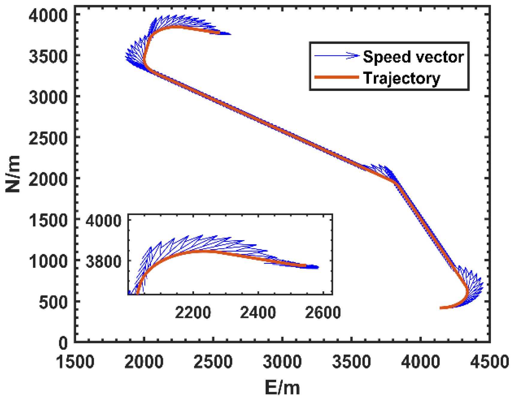
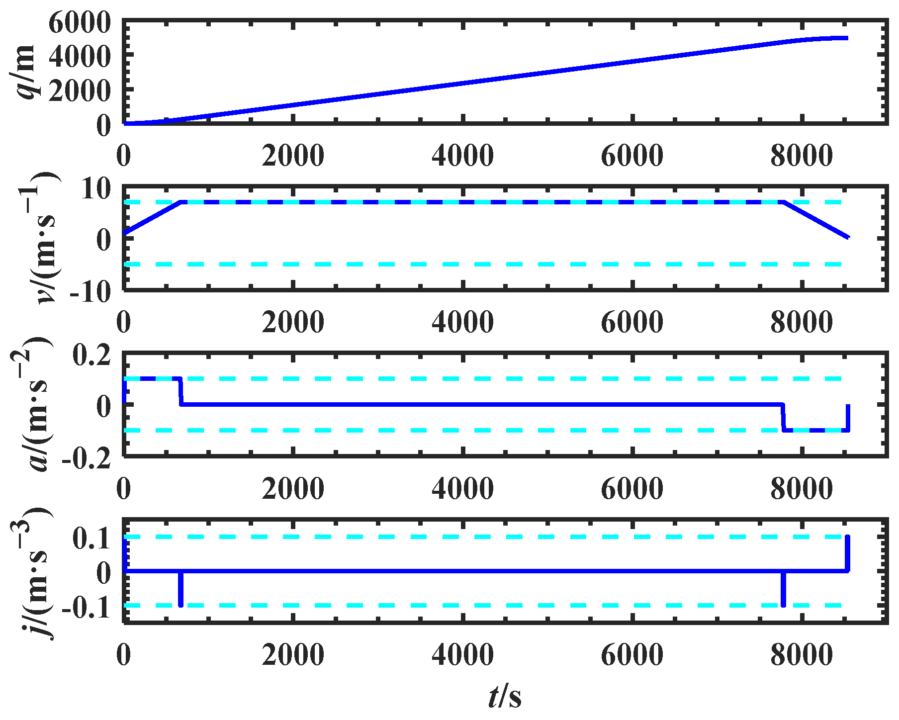
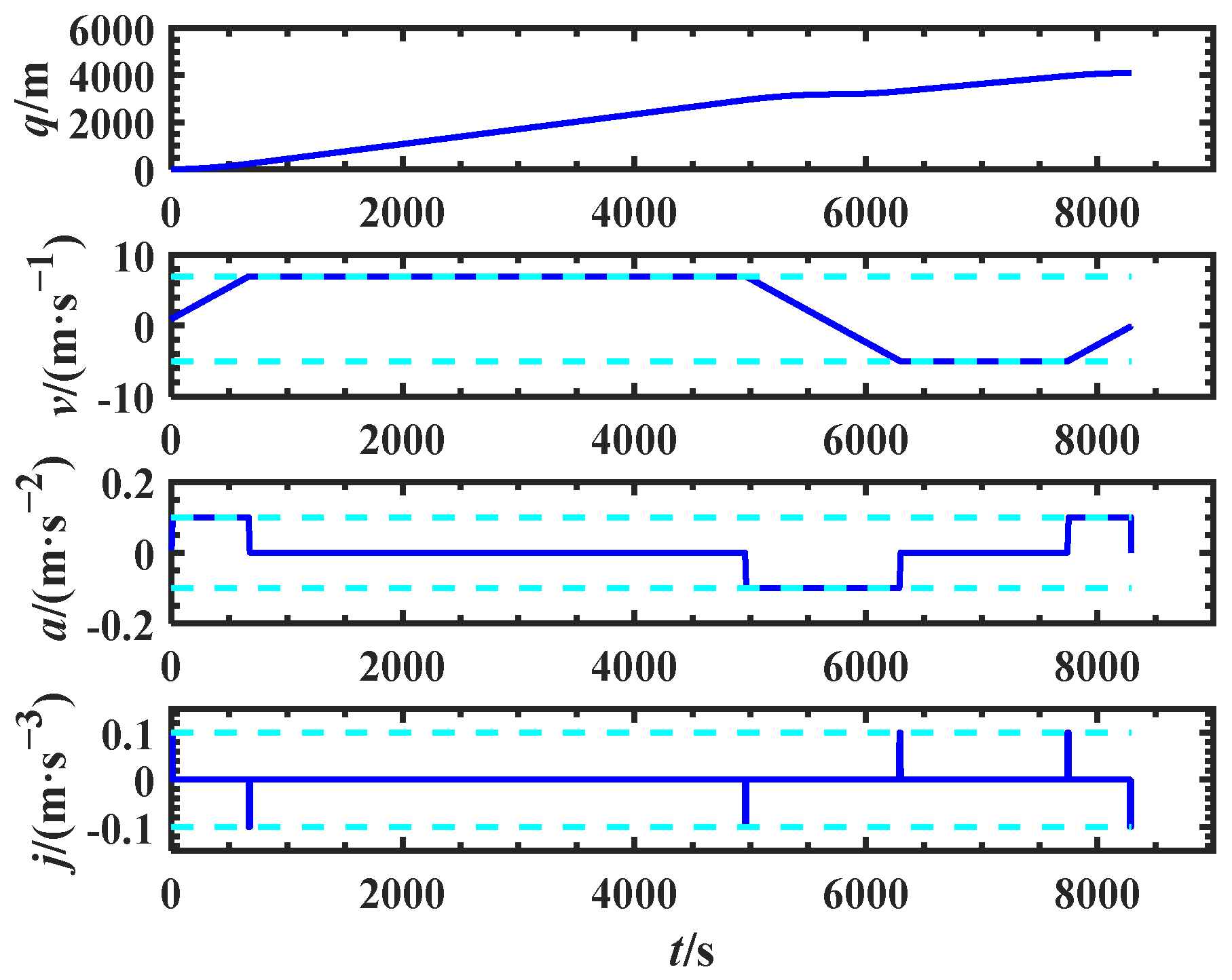
For the path derived by the multi-scale A* algorithm with RSC in Figure 8, the trajectory is planned as Figure 13 and the position, velocity, acceleration, and jerk profiles are given in Figure 14, with constraints v max = 7 , v min = 5 , a max = a min = 0.1 , j max = j min = 0.1 , and time interval Ts = 0.1. The planned trajectory is smooth and satisfies the constraints.
The proposed scheme not only satisfies the requirement of forward navigation, but is also applicable for the navigation with forward and backward motions. When the final course orients outside of the port, the planned path may have segments with backward motion, as Figure 15 illustrates, where maximum curvature is set as 0.005, initial pose [x0, y0, Ψ0] = [4138, 417, 0], and final pose [x2, y2, Ψ2] = [3500, 3330, 0]. The corresponding motion configuration is given in Figure 16. The planned trajectory meets the constraints and realizes backward motion planning.

5. Discussions

The time-related trajectory is available as per the given steps. To summarize and make the structure clearer, Figure 17 illustrates the information flow of the whole process.
As shown in Figure 17, the proposed method is quite straightforward and easily understood. The strengths and weaknesses (potential enhancement) of this method can be summarized as follows:
(1)
Strengths: high efficiency, constraints applicable (kinodynamic and nonholonomic constraints), easy to understand, suitable for motion planning including backward motions;
(2)
Weaknesses or potential enhancements: dynamic map is not suitable, no adaptive change of quad-tree structure, additional costs on environmental situation such as wind and wave are not considered.

6. Conclusions

In this research, a trajectory-planning scheme is proposed that combines multi-scale A*, RSC, and online double S trajectory planning. Only the initial and final states are needed to derive a feasible trajectory. Berthing at Long Beach Harbor is taken as an example. Both alongside and astern berthing satisfy the constraints. The length of the path is reasonable, and the safety of the path is guaranteed by the minimum grid size, which is decided by the quad-tree depth. Compared to the grid-based A* algorithm, the proposed method is fast and is able to produce paths that stay well clear of obstacles. The trajectory can be used in the control process directly to facilitate various control algorithms, by providing time-related references such as position, course, speed, and acceleration. This application is quite common in the field of vehicle motion control and manipulator systems. One can also use it to define the trajectories of actuators to avoid vibration.

Author Contributions

Conceptualization, X.H.; methodology, X.H.; validation, X.Z. and H.Z.; writing—original draft preparation, X.H.; writing—review and editing, X.H. and X.Z.; visualization, X.H. and H.Z.; supervision, X.Z.; project administration, X.Z.; funding acquisition, X.Z. All authors have read and agreed to the published version of the manuscript.

Funding

This work was funded by the National Natural Science Foundation of China (grant no. 51679024 and 51779029), and Cultivation Program for the Excellent Doctoral Dissertation of Dalian Maritime University (2022YBPY001).

Institutional Review Board Statement

Not applicable.

Informed Consent Statement

Not applicable.

Data Availability Statement

Not applicable.

Acknowledgments

The authors would like to thank anonymous reviewers for their valuable comments to improve the quality of this article.

Conflicts of Interest

The authors declare no conflict of interest.

References

  1. Mou, J.; He, Y.; Zhang, B.; Li, S.; Xiong, Y. Path Following of a Water-Jetted USV Based on Maneuverability Tests. J. Mar. Sci. Eng. 2020, 8, 354. [Google Scholar] [CrossRef]
  2. Zhang, G.; Han, J.; Li, J.; Zhang, X. APF-Based Intelligent Navigation Approach for USV in Presence of Mixed Potential Directions: Guidance and Control Design. Ocean Eng. 2022, 260, 111972. [Google Scholar] [CrossRef]
  3. Zhang, G.; Deng, Y.; Zhang, W. Robust Neural Path-Following Control for Underactuated Ships with the DVS Obstacles Avoidance Guidance. Ocean Eng. 2017, 143, 198–208. [Google Scholar] [CrossRef]
  4. Han, X.; Zhang, X. Tracking Control of Ship at Sea Based on MPC with Virtual Ship Bunch under Frenet Frame. Ocean Eng. 2022, 247, 110737. [Google Scholar] [CrossRef]
  5. Werling, M.; Kammel, S.; Ziegler, J.; Groell, L. Optimal Trajectories for Time-Critical Street Scenarios Using Discretized Terminal Manifolds. Int. J. Robot. Res. 2012, 31, 346–359. [Google Scholar] [CrossRef]
  6. Song, R.; Liu, Y.; Bucknall, R. Smoothed A* Algorithm for Practical Unmanned Surface Vehicle Path Planning. Appl. Ocean Res. 2019, 83, 9–20. [Google Scholar] [CrossRef]
  7. Xie, L.; Xue, S.; Zhang, J.; Zhang, M.; Tian, W.; Haugen, S. A Path Planning Approach Based on Multi-Direction A* Algorithm for Ships Navigating within Wind Farm Waters. Ocean Eng. 2019, 184, 311–322. [Google Scholar] [CrossRef]
  8. Daniel, K.; Nash, A.; Koenig, S.; Felner, A. Theta*: Any-Angle Path Planning on Grids. J. Artif. Intell. Res. 2010, 39, 533–579. [Google Scholar] [CrossRef] [Green Version]
  9. Hu, Y.; Harabor, D.; Qin, L.; Yin, Q. Regarding Goal Bounding and Jump Point Search. J. Artif. Intell. Res. 2021, 70, 631–681. [Google Scholar] [CrossRef]
  10. Dolgov, D.; Thrun, S.; Montemerlo, M.; Diebel, J. Practical Search Techniques in Path Planning for Autonomous Driving; American Association for Artificial Intelligence: Menlo Park, CA, USA, 2008. [Google Scholar]
  11. Yu, L.; Wei, Z.; Wang, Z.; Hu, Y.; Wang, H. Path Optimization of AUV Based on Smooth-RRT Algorithm. In Proceedings of the IEEE International Conference on Mechatronics and Automation (ICMA), Takamatsu, Japan, 6–9 August 2017; pp. 1498–1502. [Google Scholar]
  12. Liang, C.; Zhang, X.; Han, X. Route Planning and Track Keeping Control for Ships Based on the Leader-Vertex Ant Colony and Nonlinear Feedback Algorithms. Appl. Ocean Res. 2020, 101, 102239. [Google Scholar] [CrossRef]
  13. Pham, Q.; Caron, S.; Lertkultanon, P.; Nakamura, Y. Admissible Velocity Propagation: Beyond Quasi-Static Path Planning for High-Dimensional Robots. Int. J. Robot. Res. 2017, 36, 44–67. [Google Scholar] [CrossRef] [Green Version]
  14. Hu, B.; Cao, Z.; Zhou, M. An Efficient RRT-Based Framework for Planning Short and Smooth Wheeled Robot Motion Under Kinodynamic Constraints. IEEE Trans. Ind. Electron. 2021, 68, 3292–3302. [Google Scholar] [CrossRef]
  15. Biagiotti, L.; Melchiorri, C. Trajectory Planning for Automatic Machines and Robots; Springer: Berlin/Heidelberg, Germany, 2008; ISBN 978-3-540-85628-3. [Google Scholar]
  16. Kim, J.; Lim, K.; Kim, J. Auto Parking Path Planning System Using Modified Reeds-Shepp Curve Algorithm. In Proceedings of the 2014 11th International Conference on Ubiquitous Robots and Ambient Intelligence (URAI), Kuala Lumpur, Malaysia, 12–15 November 2014; pp. 311–315. [Google Scholar]
  17. Vautier, U.; Viel, C.; Wan, J.; Jaulin, L.; Hone, R.; Dai, M. Restricted Orientation Dubins Path with Application to Sailboats. IEEE Robot. Autom. Lett. 2019, 4, 4515–4522. [Google Scholar] [CrossRef] [Green Version]
  18. Zhou, Y.; Xi, J.; Luo, C. A Fast Bi-Directional A* Algorithm Based on Quad-Tree Decomposition and Hierarchical Map. IEEE Access 2021, 9, 102877–102885. [Google Scholar] [CrossRef]
  19. Philipp, K.; Marco, S.; Stefan, M.; Andreas, N. Traversability Analysis for Wheeled Robots Using Point-Region-Quad-Tree Based Elevation Maps. In Proceedings of the 2022 IEEE International Conference on Autonomous Robot Systems and Competitions (ICARSC), Santa Maria de Feira, Portugal, 29–30 April 2022; pp. 192–197. [Google Scholar]
  20. Xue, M.; Wei, M. Small Unmanned Aerial Vehicle Flight Planning in Urban Environments. J. Aerosp. Inf. Syst. 2021, 18, 702–710. [Google Scholar] [CrossRef]
  21. Han, X.; Zhang, X. Multi-Scale Theta* Algorithm for the Path Planning of Unmanned Surface Vehicle. Proc. Inst. Mech. Eng. Part M J. Eng. Marit. Environ. 2021, 236, 427–435. [Google Scholar] [CrossRef]
  22. Yang, K.; Sukkarieh, S. An Analytical Continuous-Curvature Path-Smoothing Algorithm. IEEE Trans. Robot. 2010, 26, 561–568. [Google Scholar] [CrossRef]
  23. Reeds, J.A.; Shepp, L.A. Optimal Paths for a Car That Goes Both Forwards and Backwards. Pac. J. Math. 1990, 145, 367–393. [Google Scholar] [CrossRef]
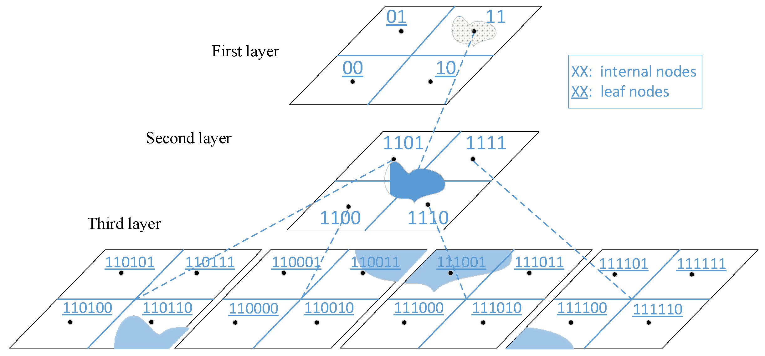
Figure 1. Structure of quad-tree with maximum layer depth 3.
Jmse 11 00153 g001
Figure 2. Two sight line discretization scheme. (a) Simple sight line discretization (sometimes obstacle node cannot be detected). (b) Safe sight line discretization (obstacle node is guaranteed to be detected).
Jmse 11 00153 g002
Figure 3. A part of Long Beach Harbor.
Jmse 11 00153 g003
Figure 4. Multi-scale graph with maximum layer depth 7.
Jmse 11 00153 g004
Figure 5. Path planned by multi-scale A* algorithm.
Jmse 11 00153 g005
Figure 6. Path planned by modified multi-scale A* algorithm.
Jmse 11 00153 g006
Figure 7. The effect of G2CBS path-smoothing algorithm.
Jmse 11 00153 g007
Figure 8. Path planned through multi-scale A* algorithm with RSC.
Jmse 11 00153 g008
Figure 9. Path planned through smooth-RRT method.
Jmse 11 00153 g009
Figure 10. Path planned using JPS with a grid cell size of 10 m.
Jmse 11 00153 g010
Figure 11. Block diagram of the trajectory planner.
Jmse 11 00153 g011
Figure 12. Typical profiles for position, velocity, acceleration, and jerk for the double S trajectory.
Jmse 11 00153 g012
Figure 13. Planned trajectory with proposed scheme.
Jmse 11 00153 g013
Figure 14. Planned profiles for position, velocity, acceleration, and jerk.
Jmse 11 00153 g014
Figure 15. Path planned with backward motion.
Jmse 11 00153 g015
Figure 16. Planned profiles for position, velocity, acceleration, and jerk including backward motion.
Jmse 11 00153 g016
Figure 17. Information flow of proposed trajectory planning method.
Jmse 11 00153 g017
Table 1. Comparison to common planning algorithms.
AlgorithmsPath Length
(m)
Time Used
(s)
Nodes ExpandedAre Constraints Met
Proposed method4962.73.368Yes
Smooth-RRT5617.674.0549Yes
JPS4655.41.721No
Disclaimer/Publisher’s Note: The statements, opinions and data contained in all publications are solely those of the individual author(s) and contributor(s) and not of MDPI and/or the editor(s). MDPI and/or the editor(s) disclaim responsibility for any injury to people or property resulting from any ideas, methods, instructions or products referred to in the content.