Article

Formation Control of Unmanned Surface Vehicles Using Fixed-Time Non-Singular Terminal Sliding Mode Strategy

Institute of Artificial Intelligence and Marine Robotics, Dalian Maritime University, Dalian 116026, China
*
Author to whom correspondence should be addressed.
J. Mar. Sci. Eng. 2022, 10(9), 1308; https://doi.org/10.3390/jmse10091308
Submission received: 26 July 2022 / Revised: 13 September 2022 / Accepted: 14 September 2022 / Published: 15 September 2022

Abstract

:
Unmanned surface vehicles (USVs) have been widely applied in the fields of marine hydrological exploration, marine resource exploration, area search, target detection, and military operations. In order to meet the demand of a complex ocean environment, USVs are frequently grouped together to improve the reliability of mission accomplishment. In this paper, a fixed-time control strategy, combined with a non-singular terminal sliding mode, is proposed for the formation control of USVs under complex external disturbances and system uncertainties. The main contributions of this paper are: (1) the leader–follower formation control framework is divided into a tracking control subsystem and a formation control subsystem. A new fixed-time non-singular terminal sliding mode (FTNTSM) strategy is developed for the tracking control subsystem, which dramatically increases the convergence rate and ensures closed-loop fixed-time stability; (2) a finite-time uncertain observer (FUO) is designed to observe lumped uncertainty items, which greatly increase the stability and robustness of the formation system; (3) the FUO-based fixed-time formation control (FUOFT-FC) strategy is designed for the formation control subsystem, which ensures the fast and stable formation of USVs. Fixed-time convergence of the formation system is established by Lyapunov stability analysis. Rigorous simulation and comparative studies demonstrate that the proposed method is superior to the state-of-the-art methods.

1. Introduction

In recent years, unmanned surface vehicles (USVs) have played an increasingly important role for mankind to explore and discover the mysteries of the ocean. USVs have been widely applied in the fields of marine hydrological exploration, marine resource exploration, area search, target detection, and military operation [1,2]. In order to deal with task diversification of USVs under complex and dynamic sea environments, USVs are frequently grouped into a unified formation to improve the reliability of mission accomplishment, which enhances fault tolerance, robustness and adaptability [3,4,5]. The common multi-agent formation control methods are leader–follower control [6], the behavior-based method [7,8], virtual structure method [9], graph theory [10,11], and consistency-based method [12]. The leader–follower control strategy can compensate well for the lack of communication in multi-agent formation and it also has a simple control structure, hence it has been widely used in formation control of USVs.
In the current USV formation control system, unmodeled dynamics and complex external disturbances bring about huge challenges to the stability of the closed-loop system. It is well-known that sliding mode control can overcome uncertainty in the system and has strong robustness, which is widely used in the field of non-linear control and multi-agent formation system [13]. Traditional sliding mode control adopts a linear sliding mode surface and uses a Lyapunov function to prove that the system can converge to an equilibrium point asymptotically. In [14,15,16], terminal sliding mode (TSM) control, which enables the system to converge to an equilibrium point in a finite time, is proposed to greatly improve system stability. Unfortunately, its convergence rate is very slow and there is a singularity problem with the designed controller. Inspired by earlier work, this paper introduces a new non-singular terminal sliding mode (NTSM) strategy for formation control of USVs to improve the system’s convergence rate and overcome singularity.
The marine environment is complex and unknown. Hence, in order to deal with internal unmodeled dynamics and complex external disturbances in the formation system, disturbance observers such as the non-linear disturbance observer, sliding mode disturbance observer, and dimensionality reduction observer are developed in [17,18,19]. In order to have a more effective and efficient observer, the finite-time disturbance observer for the marine unmanned system was developed in [20,21,22,23,24,25,26,27], which enhanced the identification of control system disturbance. However, in the aforementioned methods, disturbance estimation errors are either globally asymptotically stable or globally unified and finally bounded, without realizing accurate observation of disturbances. In this context, the finite-time uncertain observer, which can accurately and effectively identify complex disturbances in a shorter time, is proposed.
In the leader–follower USVs formation control system, in order to ensure better response of the system, the convergence rate is the most critical control index. Recently, more and more finite-time control strategies have been developed to solve the convergence problem of single-agent and multi-agent systems in [28,29,30]. The tracking accuracy and convergence rate have been greatly improved. As an extension of the finite-time algorithm of [31], the main advantage of the fixed-time control algorithm is that the initial value of the agent state need not be known a priori when calculating the upper bound of the convergence time, and a better convergence rate and convergence accuracy have been achieved. In [32,33,34], the fixed-time algorithms in first-order, second-order, and high-order multi-agent systems are developed, and better accuracy and convergence have been achieved.
Inspired by earlier work, we combine fixed-time control and non-singular terminal sliding mode control (FTNTSM) to design a fast and accurate USV formation control strategy. To be specific, a new formation control strategy based on fixed-time non-singular terminal sliding mode, which is used to deal with formation control of USVs under complex external disturbances and system uncertainties, is proposed. The main contributions of the paper are:
(1) In order to simplify the leader–follower formation control framework, the entire system is divided into two subsystems, namely the tracking control subsystem and formation control subsystem. In the tracking control subsystem, a tracking control strategy based on the fixed-time non-singular terminal sliding mode (FTNTSM-TC) is designed, which enables the leader to quickly and precisely track the desired trajectory.
(2) Unmodeled dynamics and external disturbances in the system are considered lumped uncertainty items. Next, a finite-time uncertain observer (FUO) is designed to deal with internal and external disturbances, which can accurately and effectively identify lumped uncertainty items.
(3) In the formation control subsystem, the fixed-time formation control strategy based on FUO (FUOFT-FC) is designed to improve the stability and reliability of the entire USV system. The system stability of the proposed formation control strategy is established by rigorous Lyapunov stability theory. Simulation and comparative studies demonstrate that the proposed strategy is superior to the TSM strategy in [16].
The organization of the paper is as follows: Section 2 introduces the same lemmas and mathematical formulation of the USVs formation system. Section 3 introduces the design process of the tracking control subsystem and the formation control subsystem in detail and establishes the stability of the entire closed-loop system. Section 4 presents simulation results that demonstrate the effectiveness and efficiency of the proposed control strategy. Conclusions are drawn in Section 5.

2. Preliminaries and Problem Formulation

In order to provide rigorous theoretical support for the subsequent design of the formation controller and proof of system stability, we introduce three fixed-time control lemmas and a finite-time control lemma in the first part. As shown in the sequel, these lemmas are needed for the proof of the stability of the designed fixed-time non-singular terminal sliding mode (FTNTSM) strategy and finite-time uncertain observer (FUO), as well as to enhance the reliability of the proposed algorithms. In the second part of this section, we formulate the research problem and introduce mathematical models for the formation control of USV in detail. In the sequel, these mathematical models are rigorously used in the design of the formation controller and proof of stability.

2.1. Preliminaries

Lemma 1.
Consider the following non-linear system [35]:
x ˙ ( t ) = f ( x ( t ) ) , x ( 0 ) = x 0 , f ( 0 ) = 0 , x R n
where x = [ x 1 , x 2 , , x n ] T is the system state vector and f ( · ) is a non-linear function defined in the neighborhood of the origin.
If system (1) is asymptotically stable and has a negative homogeneity degree, system (1) is finite-time stable. If the settling time function T ( ε ) is bounded by a positive constant T m a x > 0 , i.e., T ( ε ) T m a x for all ε R n , system (1) is fixed-time stable.
Lemma 2.
Consider the following scalar system [36]:
y ˙ = γ 1 y 2 p / q γ 2 y p / q , y ( 0 ) = y 0
where γ 1 , γ 2 > 0 , p , q are both positive odd integers satisfying p < q . System (2) is fixed-time stable and the upper bound of the convergence time satisfies
T m a x y 0 = q π 2 γ 1 γ 2 q p
Lemma 3.
Consider the following system [37]:
y ˙ = α y A β y B , y ( 0 ) = y 0
where A = a 1 / a 2 , B = b 1 / b 2 , a 1 , a 2 , b 1 , b 2 are positive odd integers satisfying a 1 > a 2 , b 1 < b 2 < 2 b 1 and α > 0 , β > 0 . The equilibrium point of the system is fixed-time stable and the upper bound of the convergence time can be calculated independently of the initial state by:
T m a x = a 2 α ( a 1 a 2 ) + b 2 β ( b 2 b 1 )
Lemma 4.
Consider the following smooth non-linear system [38]:
σ ˙ 0 = λ 0 L 1 / n + 1 | σ 0 | n / ( n + 1 ) sgn σ 0 + σ 1 σ ˙ 1 = λ 1 L 1 / n + 1 | σ 1 σ ˙ 0 | ( n 1 ) / n sgn ( σ 1 σ ˙ 0 ) + σ 2 σ ˙ n 1 = λ n 1 L 1 / 2 | σ n 1 σ ˙ n 2 | 1 / 2 sgn ( σ n 1 σ ˙ n 2 ) + σ n σ ˙ n λ n L sgn ( σ σ ˙ n 1 ) + L , L
where L > 0 is the known Lipshitz constant, λ i > 0 , ( i = 0 , 1 , 2 , , n ) are appropriate constants, sgn ( · ) is the signum function, and the σ i ( i = 0 , 1 , 2 , , n ) are sliding variable without noise. We call the system finite-time stable if it is asymptotically stable with a finite settling time for the initial conditions.

2.2. Problem Formulation

Although the six-degrees-of-freedom model can comprehensively reflect the kinematic characteristics of the USV, the actual actuator cannot fully control the six degrees of freedom under normal circumstances. Therefore, in this paper, we only consider the three-degrees-of-freedom USV model consisting of the surge speed u, the sway speed v , and the yaw angular speed r.
As shown in Figure 1, the USV model with disturbances and position dynamics is governed by:
η ˙ i = R ( ψ i ) ν i M i ν ˙ i + g ( η ) = B ( η i , ν i ) + τ i + δ i
where
B ( η i , ν i ) = C ( ν i ) ν i D ( ν i ) ν i
i = 0 represents the kinematics and dynamics of the leader USV; i = 1 , 2 , , n represent the kinematics and dynamics of a follower USV; η i = [ x i , y i , ψ i ] T denotes the USV’s position and heading angle vector in the earth-fixed coordinate; ν i = [ u i , v i , r i ] T denotes the surging speed u, the swaying speed v, and the yawing angular speed r vectors in the body-fixed coordinate; τ i = [ τ i 1 , τ i 2 , τ i 3 ] T denotes control input vector of the leader or follower; δ i = M i R T ( ψ i ) d i ( t ) , d i ( t ) denotes external disturbances; B ( · ) represents the hydrodynamic characteristics of the position of a USV under unknown sea condition; g ( η ) represents the force and moment of buoyancy and gravity of the USVs (ideal state g ( η ) = 0 ); R ( ψ i ) is a rotation matrix; M i = M i T > 0 is an inertia matrix; C ( ν i ) = C ( ν i ) T is a skew-symmetric matrix; D ( ν i ) is a damping matrix.
R ( ψ ) = cos ψ sin ψ 0 sin ψ cos ψ 0 0 0 1
M = m 11 0 0 0 m 22 m 23 0 m 32 m 33
C ( ν ) = 0 0 c 13 ( ν ) 0 0 c 23 ( ν ) c 13 ( ν ) c 23 ( ν ) 0
D ( ν ) = d 11 ( ν ) 0 0 0 d 22 ( ν ) d 23 ( ν ) 0 d 32 ( ν ) d 33 ( ν )
The rotation matrix R ( ψ ) satisfies the following properties:
R ˙ ( ψ ) = R ( ψ ) S ( r ) R T ( ψ ) S ( r ) R ( ψ ) = R ( ψ ) S ( r ) R T ( ψ ) = S ( r ) R ( ψ ) = 1 , R T ( ψ ) R ( ψ ) = I , ψ [ 0 , 2 π ]
where
S ( r ) = 0 r 0 r 0 0 0 0 0
Definitions of matrix parameters are shown in Table 1. The term m is the mass of the USV, B is the width of the USV, I z is the moment of inertia, and x g is the coordinate value of the center of USV ’s gravity on the body-fitted coordinate systems, N v ˙ = Y r ˙ and X , Y , Z denote the hydrodynamic derivatives.
Consider the following desired trajectory:
η ˙ d = R ( ψ d ) ν d M ν ˙ d = E ( η d , ν d ) + τ d
where
E ( η d , ν d ) = C ( ν d ) ν d D ( ν d ) ν d
and η d = [ x d , y d , ψ d ] T , ν d = [ u d , v d , r d ] T denote the desired position vector and velocity vector respectively and τ d = [ τ d 1 , τ d 2 , τ d 3 ] T .
In Section 2, we have introduced the lemmas needed for stability proof and basic mathematical models for formation control of USVs. As foreshadowed, these results lay the foundation for subsequent design and analysis. Next, we design the formation controller and disturbance observer as well as state two main results pertaining to tracking the performance of the designed formation controller in finite time.

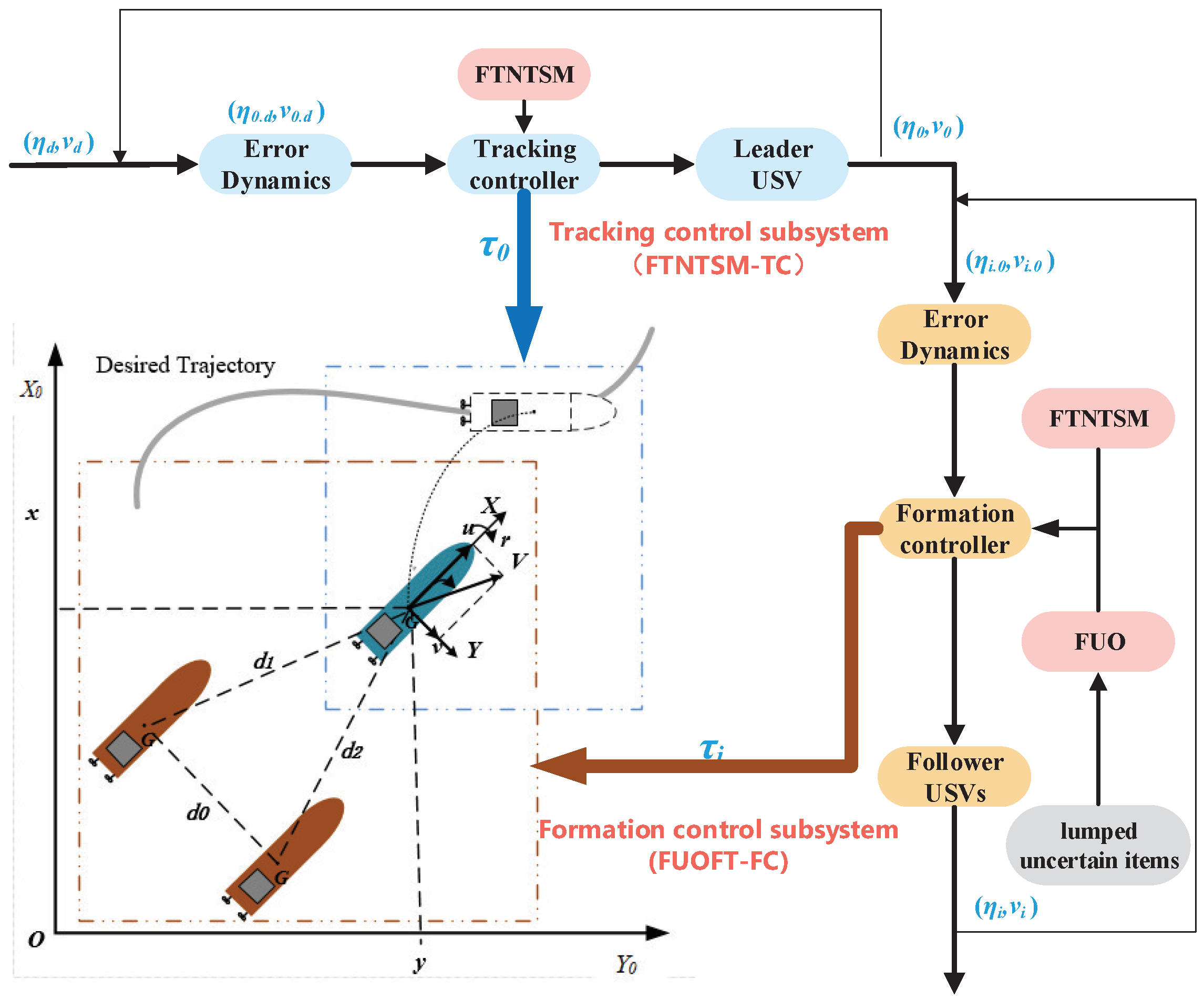
3. Design of Formation Control Strategy

In this paper, the formation system is divided into a tracking control subsystem and a formation control subsystem, and control strategies are designed separately to ensure the efficiency and effectiveness of the formation system.
It is assumed that complex external disturbances of the formation control subsystem have an upper bound i.e., d ˙ i Z i ; ( Z i < ) .
To facilitate the following analysis, we introduce auxiliary variables χ i ,   χ d as follows:
χ i = R i ν i χ d = R d ν d
where χ i = [ χ i , 1 , χ i , 2 , χ i , 3 ] T , χ d = [ χ d , 1 , χ d , 2 , χ d , 3 ] T , R i = R ( ψ i ) and R d = R ( ψ d ) . Then, the following coordinate transformation can be obtained:
η ˙ i = χ i χ ˙ i = R i M i 1 τ i + F ( η i , χ i ) + d i ( t )
and
F ( η i , χ i ) = S ( χ i 3 ) χ i + R i M i 1 B ( η i , R i T χ i ) .
η ˙ d = χ d χ ˙ d = R d M d 1 τ d + H ( η d , χ d )
and
H ( η d , χ d ) = S ( χ d 3 ) χ d + R d M d 1 Z ( η d , R d T χ d ) .

3.1. Design of Tracking Control Subsystem and Stability Analysis

Figure 2 is a block diagram of the USV formation control system. Combining (18) and (20), the tracking error dynamics between the leader and the desired trajectory are governed by:
η ˙ 0 , d = χ 0 , d χ ˙ 0 , d = I e + R 0 M 0 1 τ 0
where
I e = F ( η 0 , χ 0 ) H ( η d , χ d ) R d M d 1 τ d
and η 0 , d = η 0 η d , χ 0 , d = χ 0 χ d , respectively, represent the position error vector and velocity error vector after coordinate transformation.
Given η 0 , d , χ 0 , d , design the FTNTSM as follows:
ζ ( t ) = η 0 , d + [ ( α η 0 , d A B + β ) 1 χ 0 , d ] 1 B
where A = a 1 a 2 , B = b 1 b 2 ; α , β > 0 ; a 1 , a 2 , b 1 , b 2 are positive odd integers and satisfy a 1 > a 2 , b 1 < b 2 < 2 b 1 , A B > 1 .
The time derivative of the sliding surface is given by
ζ ˙ ( t ) = χ 0 , d + 1 B [ ( α η 0 , d A B + β ) 1 χ 0 , d ] 1 B 1 [ ( α η 0 , d A B + β ) 2 α ( A B ) η 0 , d A B 1 χ 0 , d 2 + ( α η 0 , d A B + β ) 1 χ ˙ 0 , d ]
Let Φ = ( α η 0 , d A B + β ) 1 , we have:
ζ ˙ ( t ) = χ 0 , d + 1 B [ Φ χ 0 , d ] 1 B 1 [ α ( A B ) η 0 , d A B 1 Φ 2 χ 0 , d 2 + Φ χ ˙ 0 , d ]
According to Lemma 2, combining (22) and (24), we have
ζ ˙ ( t ) = χ 0 , d + 1 B [ Φ χ 0 , d ] 1 B 1 [ α ( A B ) η 0 , d A B 1 Φ 2 χ 0 , d 2 + Φ ( I e + R 0 M 0 1 τ 0 ) ] = λ 0 ζ λ 1 ζ 2 m / n λ 2 ζ m / n
where λ 0 , λ 1 , λ 2 > 0 .
Let κ = λ 0 ζ λ 1 ζ 2 m / n λ 2 ζ m / n . Then, the tracking control strategy based on fixed-time fast terminal sliding mode (FTNTSM-TC) is designed as follows:
τ 0 = M 0 R 0 1 [ ( κ χ 0 , d ) B χ 0 , d ( Φ χ 0 , d ) 1 B + α ( A B ) η 0 , d A B 1 Φ χ 0 , d 2 I e ]
Now, we state the main result of this work.
Theorem 1.
Consider the USV tracking control system governed by (22) under the assumption that there are no lumped disturbances, the tracking control strategy (28) is able to ensure that the leader tracks the desired trajectory precisely. Moreover, the convergence time is independent of the initial state of the leader, and the upper bound of the convergence time is given by
T s = T 0 , m a x + T 1 , m a x
Proof of Theorem 1. 
Reaching phase: Select the following Lyapunov function:
V 1 = 1 2 ζ T ζ
Combining (27) and (28), the derivative of (30) can be obtained as follows:
V ˙ 1 = ζ T ζ ˙ = ζ T [ χ 0 , d + 1 B [ Φ χ 0 , d ] 1 B 1 [ α ( A B ) η 0 , d A B 1 Φ 2 χ 0 , d 2 + Φ χ 0 , d ˙ ] ] = ζ T [ χ 0 , d + 1 B [ Φ χ 0 , d ] 1 B 1 [ α ( A B ) η 0 , d A B 1 Φ 2 χ 0 , d 2 + Φ ( I e + R 0 M 0 1 τ 0 ) ] ] = ζ T [ λ 0 ζ + λ 1 ζ 2 m / n + λ 2 ζ m / n ] = λ 0 ζ 2 λ 1 2 3 n m 2 n ( 1 2 ζ 2 ) 3 n m 2 n λ 2 2 n + m 2 n ( 1 2 ζ 2 ) n + m 2 n λ 1 2 3 n m 2 n V 1 2 m + n 2 n λ 2 2 n + m 2 n V 1 m + n 2 n μ 1 V 1 2 ϖ 1 / θ 1 μ 2 V 1 ϖ 1 / θ 1
where μ 1 = λ 1 2 3 n m 2 n , μ 2 = λ 2 2 n + m 2 n , ϖ 1 = m + n , θ 1 = 2 n , and ϖ 1 < θ 1 .
Using Lemma 2, the upper bound of the convergence time can be calculated as follows:
T 1 , m a x = ϖ 1 π 2 μ 1 μ 2 ( ϖ 1 θ 1 )
Hence, the designed fixed-time non-singular terminal sliding surface can be reached within a fixed time. Then, the error vectors η 0 , d , χ 0 , d converge to the sliding surface, we can obtain ζ ( t ) = 0 , ζ ˙ ( t ) = 0 .
ζ ( t ) = η 0 , d + [ ( α η 0 , d A B + β ) 1 χ 0 , d ] 1 B = 0
After simplification, we have
χ 0 , d = η ˙ 0 , d = α η 0 , d A β η 0 , d B
According to Lemma 3, after reaching the sliding stage, the upper bound of the convergence time satisfies the following inequality:
T 0 , max = 1 α a 2 a 1 a 2 + 1 β b 2 b 2 b 1
According to (29), the upper bound of the convergence time does not depend on the initial state of the leader and is given by T s = T 0 , m a x + T 1 , m a x .
Theorem 1 is proven complete. □

3.2. Design of Formation Control Subsystem and Stability Analysis

The unmodeled dynamics and external disturbances in each follower of the formation control subsystem will be regarded as lumped uncertain items f i u ( · ) .
For the formation control subsystem, the formation control error is rewritten as follows:
η ˙ i , 0 = χ i , 0 χ ˙ i , 0 = R i M i 1 τ i + S i χ i S 0 χ 0 + f i u ( · )
where
f i u ( · ) = R i M i 1 B i R 0 M 0 1 B 0 + d i ( t )
and f i u ( · ) denotes lumped uncertainty items, and B i = B ( η i , ν i ) , B 0 ( · ) = B ( η 0 , ν 0 ) .
Let ω i , 1 be the observed value of disturbance f i u . We design a finite-time uncertain observer (FUO) as follows:
w ˙ i , 0 = S i χ i S 0 χ 0 + R i M i 1 τ i + ξ i , 0 ξ i , 0 = λ i , 3 Z i 1 / 3 sig 2 / 3 ( w i , 0 χ i , 0 ) + w i , 1 w ˙ i , 1 = ξ i , 1 ξ i , 1 = λ i , 4 Z i 1 / 2 sig 1 / 2 ( w i , 1 ξ i , 0 ) + w i , 2 w ˙ i , 2 = λ i , 5 Z i sgn ( w i , 2 ξ i , 1 )
where w i , j : = [ w i , j , 1 , w i , j , 2 , w i , j , 3 ] T ,   j = 0 , 1 , 2 , ξ i , k : = [ ξ i , k , 1 , ξ i , k , 2 , ξ i , k , 3 ] T ( k = 0 , 1 ) is the disturbance observer state, λ i , j > 0 ,   j = 3 , 4 , 5 , and Z i = d i a g ( z i 1 , z i 2 , z i 3 ) is the designed parameter of the observer.
The observation errors of the disturbance observer are defined as follows:
e i , 1 = w i , 0 χ i , 0 e i , 2 = w i , 1 d i e i , 3 = w i , 2 d ˙ i
The time derivatives of system (39) are obtained as follows:
e ˙ i , 1 = λ i , 3 Z i 1 / 3 sig 2 / 3 ( e i , 1 ) + e i , 2 e ˙ i , 2 = λ i , 4 Z i 1 / 2 sig 1 / 2 ( e i , 2 e ˙ i , 1 ) + e i , 3 e ˙ i , 3 = λ i , 5 Z i sgn ( e i , 3 e ˙ i , 2 ) d ¨ i
According to Lemma 4, the observation error system (40) is stable for a finite time. When the disturbance is effectively observed, we have:
w i , 0 ( t ) χ i , 0 ( t ) , w i , 1 ( t ) d i ( t ) , w i , 2 ( t ) d ˙ i ( t )
Given η i , 0 , χ i , 0 , design the FTNTSM as follows:
ε ( t ) = η i , 0 + [ ( α η i , 0 A B + β ) 1 χ i , 0 ] 1 B
where A = a 1 a 2 , B = b 1 b 2 ; α , β > 0 ; a 1 , a 2 , b 1 , b 2 are positive odd integers and satisfy a 1 > a 2 , b 1 < b 2 < 2 b 1 , A B > 1 .
The time derivative of the sliding surface is governed by:
ε ˙ ( t ) = χ i , 0 + 1 B [ ( α η i , 0 A B + β ) 1 χ i , 0 ] 1 B 1 [ ( α η i , 0 A B + β ) 2 α ( A B ) η i , 0 A B 1 χ i , 0 2 + ( α η i , 0 A B + β ) 1 χ ˙ i , 0 ]
Let Φ i = ( α η i , 0 A B + β ) 1 , we have
ε ˙ ( t ) = χ i , 0 + 1 B [ Φ i χ i , 0 ] 1 B 1 [ α ( A B ) η i , 0 A B 1 Φ i 2 χ i , 0 2 + Φ i χ ˙ i , 0 ]
According to Lemma (2), combining (36) and (42), we have
ε ˙ ( t ) = χ i , 0 + 1 B [ Φ i χ i , 0 ] 1 B 1 [ α ( A B ) η i , 0 A B 1 Φ i 2 χ i , 0 2 + Φ i ( S i χ i S 0 χ 0 + ω i , 1 + R i M i 1 τ i ) ] = λ i , 0 ε λ i , 1 ε 2 p / q λ i , 2 ε p / q
where λ i , 0 , λ i , 1 , λ i , 2 > 0 and p , q are positive odd numbers satisfying p < q .
Let κ i = λ i , 0 ε λ i , 1 ε 2 p / q λ i , 2 ε p / q . Furthermore, the FUO-based fixed-time formation control (FUOFT-FC) strategy is designed as follows:
τ i = M i R i 1 [ ( κ χ i , 0 ) B χ i , 0 ( Φ i χ i , 0 ) 1 B + α ( A B ) η i , 0 A B 1 Φ i χ i , 0 2 ( S i χ i S 0 χ 0 + ω i , 1 ) ]
Concerning the identification and control of complex unknown disturbances and system uncertainties, we have the following main result.
Theorem 2.
Consider the USV formation control system with a lumped uncertainty term f i u governed by (37), the designed FUO can effectively identify f i u in a finite time. The designed FUOFT-FC strategy can rapidly and steadily maintain the desired formation in a fixed time.
Proof of Theorem 2. 
Select the following Lyapunov function:
V 2 = 1 2 ε T ε
The time derivative of system (47) is given by
V ˙ 2 = ε T ε ˙ = ε T [ χ i , 0 + 1 B [ Φ i χ i , 0 ] 1 B 1 [ α ( A B ) η i , 0 A B 1 Φ i 2 χ i , 0 2 + Φ i χ ˙ i , 0 ] ] = ε T [ χ i , 0 + 1 B [ Φ i χ i , 0 ] 1 B 1 [ α ( A B ) η i , 0 A B 1 Φ i 2 χ i , 0 2 + Φ i ( R i M i 1 τ i + S i χ i S 0 χ 0 + f i u ( · ) ) ] ] = ε T [ λ i , 0 ε + λ i , 1 ε 2 p / q + λ i , 2 ε p / q + f i u ( · ) ω i , 1 ] = λ i , 0 ε 2 λ i , 1 2 3 q p 2 q ( 1 2 ε 2 ) 3 q p 2 q λ i , 2 2 q + p 2 q ( 1 2 ε 2 ) q + p 2 q λ i , 1 2 3 q p 2 q V 3 2 q + p 2 q λ i , 2 2 q + p 2 q V 3 q + p 2 q μ i , 1 V 1 2 ϖ i , 1 / θ i , 1 μ i , 2 V 1 ϖ i , 1 / θ i , 1
where i = 1 , 2 mean followers. μ i 1 = λ i , 1 2 3 q p 2 q , μ i , 2 = λ i , 2 2 q + p 2 q , ϖ i , 1 = q + p , θ i , 1 = 2 q , and ϖ i , 1 < θ i , 1 .
Using Lemma 2, the upper bound of the convergence time can be calculated, and the designed FTNTSM strategy can be reached within a fixed time:
T i 1 , m a x = ϖ i , 1 π 2 μ i , 1 μ i , 2 ( ϖ i , 1 θ i , 1 )
Hence, the designed fixed-time non-singular terminal sliding mode can be reached within a fixed time. Then, we can obtain ε ( t ) = 0 , ε ˙ ( t ) = 0 , and
ε ( t ) = η i , 0 + [ ( α η i , 0 A B + β ) 1 χ i , 0 ] 1 B = 0
which can be simplified as follows:
χ i , 0 = η ˙ i , 0 = α η i , 0 A β η i , 0 B
According to Lemma 3, after reaching the sliding stage, the upper bound of the convergence time satisfies the following inequality:
T i 0 , max = 1 α a 2 a 1 a 2 + 1 β b 2 b 2 b 1
Theorem 2 is proven complete. □

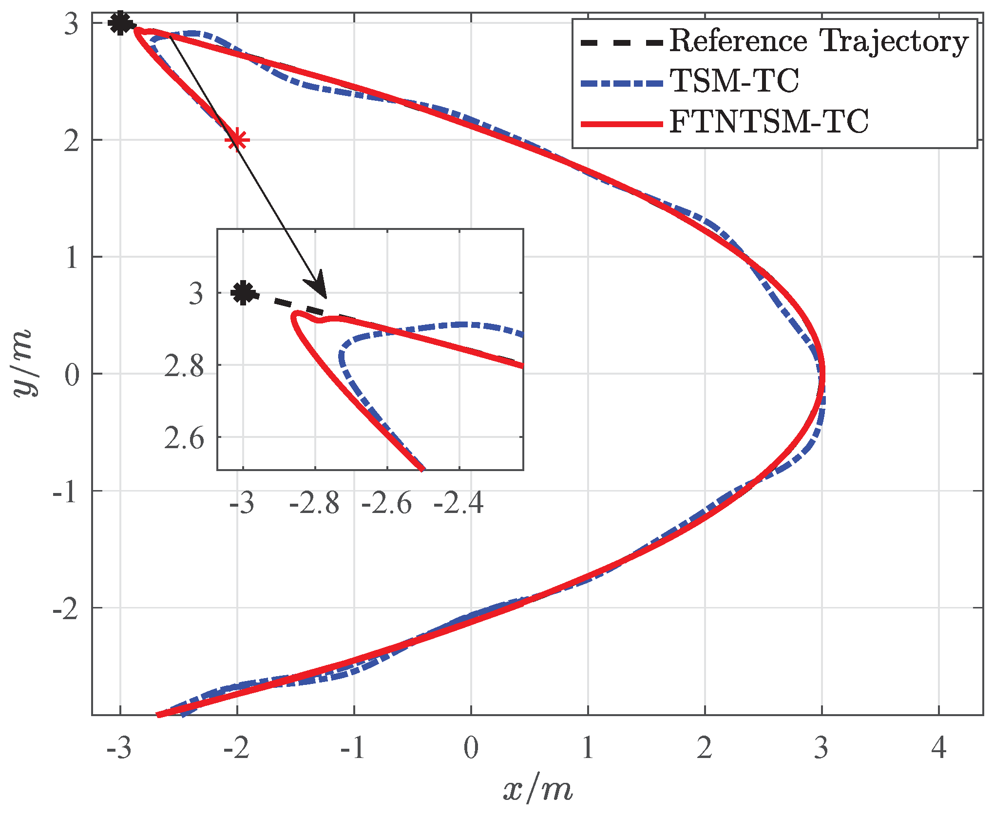
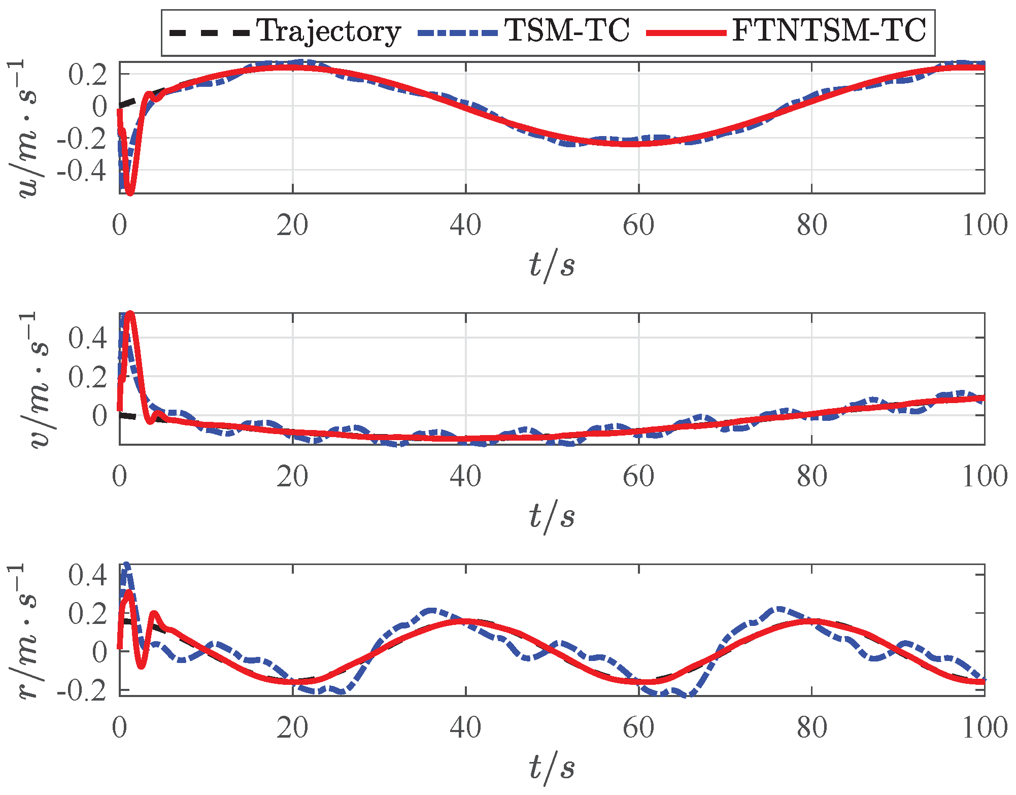
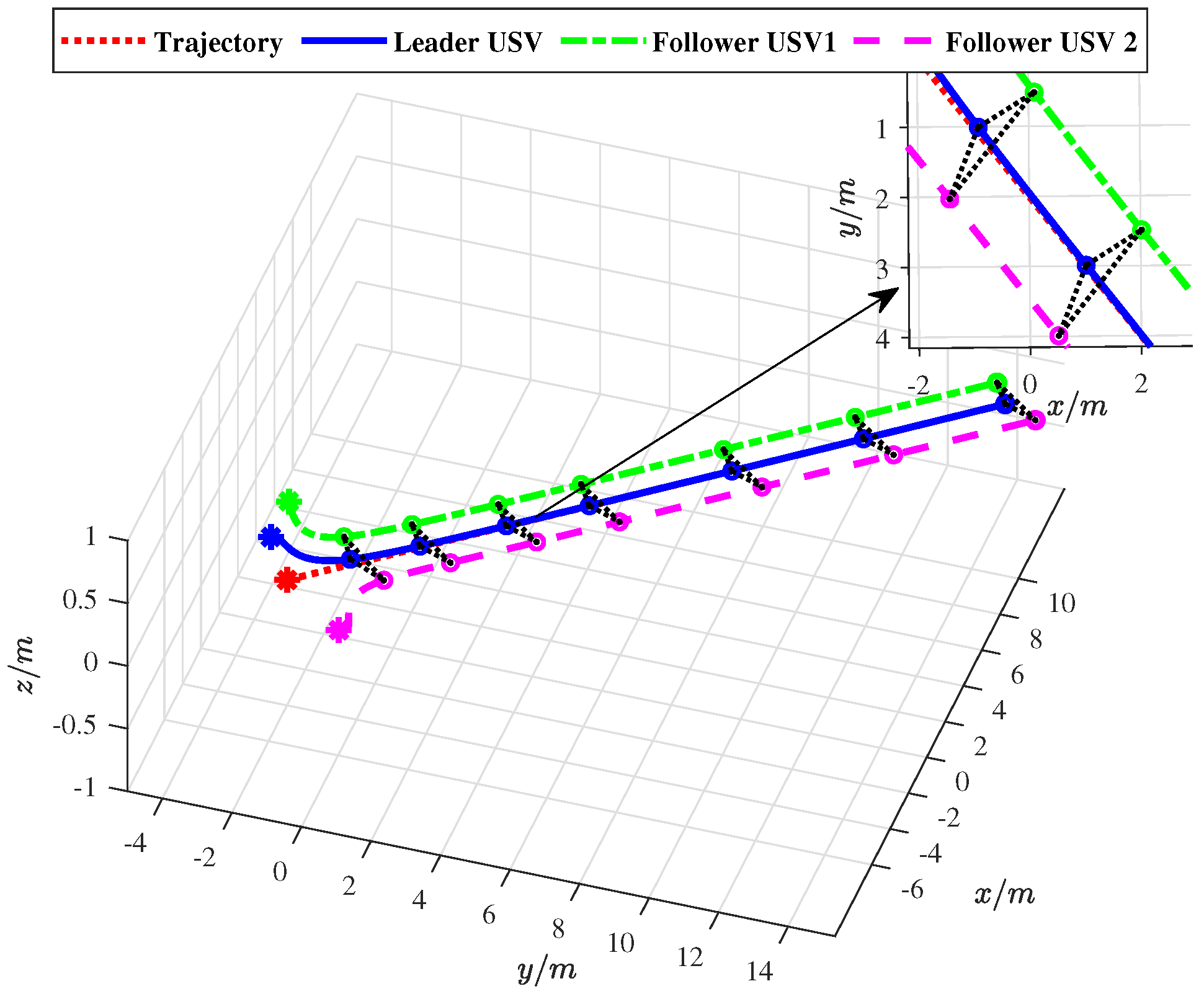
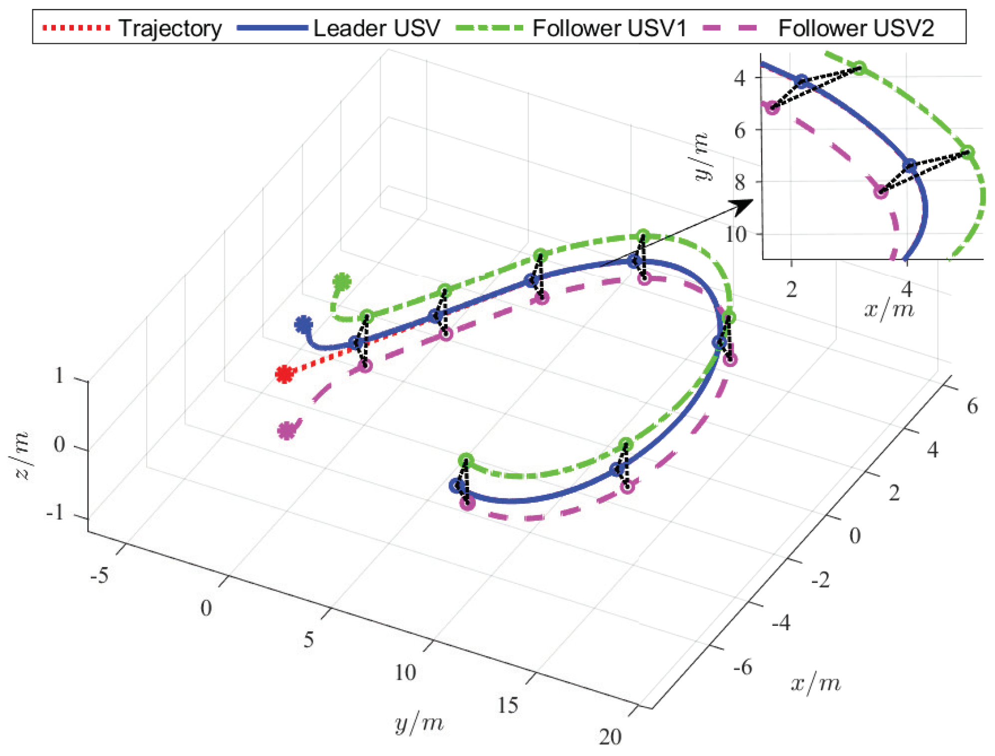
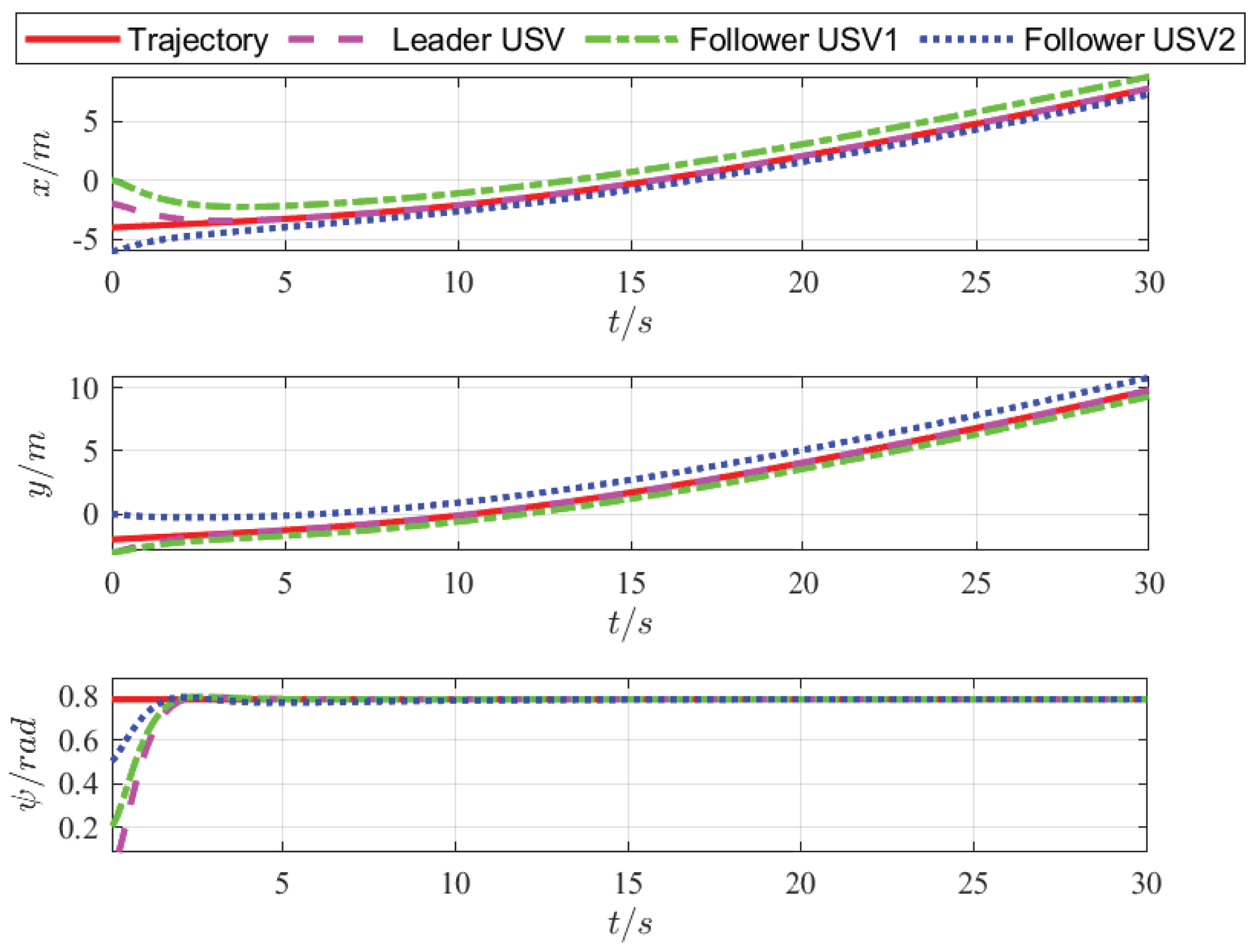
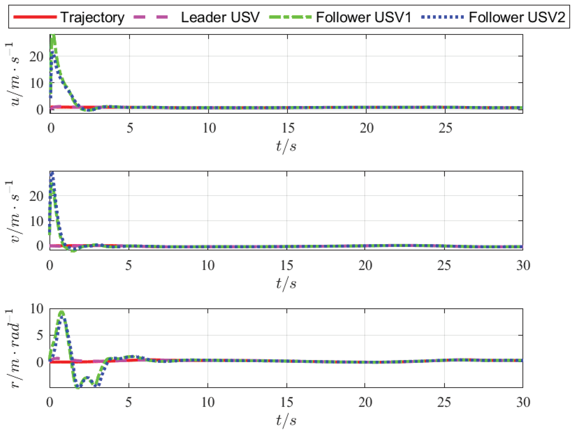
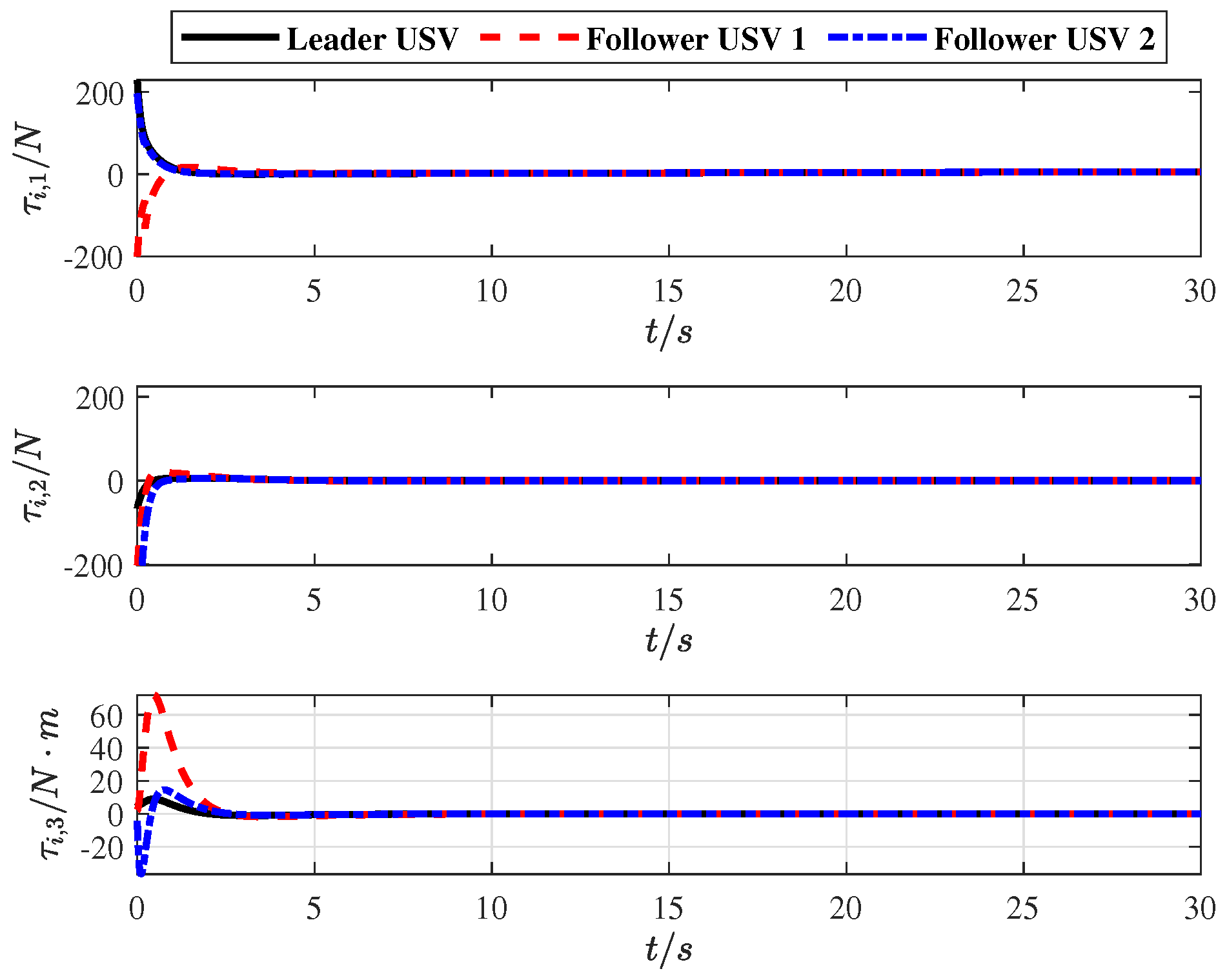
4. Simulation and Discussion

In order to verify the efficiency and effectiveness of the proposed control strategy, the classic Cybership II USV model is used for simulation studies [39]. The parameters of the Cybership II USV model are shown in Table 2. The parameters of the sliding mode control surface, disturbance observer, and formation controller are shown in Table 3. The initial values of the desired trajectory, the leader USV, and follower USVs are shown in Table 4.
The disturbance vector is governed by:
d 1 = cos ( 0 . 2 π t ) + 0 . 1 sin ( π t ) cos ( π t ) + sin ( 2 t ) cos ( π t ) + sin ( 0 . 1 t )
d 2 = cos ( 0 . 2 π t ) + 0 . 1 sin ( π t ) cos ( π t ) + sin ( 2 t ) cos ( π t ) + sin ( 0 . 1 t )
Simulation results are shown in Figure 3, Figure 4, Figure 5, Figure 6, Figure 7, Figure 8, Figure 9, Figure 10, Figure 11, Figure 12 and Figure 13. Figure 3 shows the comparison results of the proposed FTNTSM-TC strategy and TSM-TC strategy. The results show that the convergence rate and stability of the proposed FTNTSM-TC strategy are better than that of the TSM-TC strategy. Figure 4 and Figure 5 show position tracking and velocity tracking of FTNTSM-TC and TSM-TC, which further demonstrate the effectiveness and efficiency of the proposed FTNTSM-TC strategy.
Figure 6 and Figure 7 show that when the desired trajectory is a straight line, the designed tracking control strategy enables the leader to accurately track the desired trajectory and the designed formation control strategy can also enable followers to accurately track the leader and maintain a straight-line navigation formation. When the desired trajectory is a curve, the USVs can also move smoothly and maintain a stable curvature navigation formation, which verifies the closed-loop stability and effectiveness of the proposed FUOFT-FC strategy. Figure 8 and Figure 9 show the position tracking and velocity tracking of the USV formation control subsystem using the proposed strategies. The results demonstrate that the FTNTSM-TC and FUOFT-FC strategies can quickly and effectively perform tracking control and maintain stable formation in five seconds, and greatly improve the convergence rate of the system.
Figure 10 shows a smooth input tracking curve without internal and external disturbances, which further demonstrates the effectiveness and efficiency of the proposed FUOFT-FC strategy. Figure 11 shows the time evolution of the lumped uncertainty and observation disturbances by the finite-time uncertain observer. Simulation results show that the lumped uncertainty items of the system can be quickly and accurately observed, thereby demonstrating the superiority of the proposed strategy. Figure 12 shows the time evolution of the control input after the lumped uncertainty items are processed by the proposed FUO, which shows that the designed FUO can accurately identify the disturbances. Figure 13 shows the norm of the tracking errors and their derivatives. It is clear that the lumped uncertainty items can be handled efficiently by the proposed FUO.
Through the above design and analysis, it can be seen that the USV formation controller designed based on the fixed-time non-singular terminal sliding mode (FTNTSM) strategy has excellent control performance and can accurately control multiple USVs to maintain the desired formation and stable operation. At the same time, the finite-time uncertainty observer (FUO) designed in this paper has excellent anti-disturbance capabilities and is able to effectively eliminate influences of internal and external disturbances on the stability of the system. Simulation results demonstrate that excellent performances have been achieved. The design of the formation controller based on fixed-time control theory and sliding mode control theory provides an interesting and important research direction in the community of marine science and engineering.

5. Conclusions

In this paper, the FTNTSM-TC strategy and the FUOFT-FC strategy are proposed for the leader–follower USV formation system which contains complex unknown and disturbances uncertainties. We divide the entire formation control system into the tracking control subsystem and the formation control subsystem. In the tracking control subsystem, an FTNTSM-TC strategy is designed to make the leader track the desired trajectory accurately. In the formation control subsystem, the lumped uncertainly items can be accurately identified by the proposed FUO, and a FUOFT-FC strategy is designed to make the followers maintain a good relative position with the leader accurately and keep stable formation. The stability of the closed-loop formation control system is established by Lyapunov stability analysis. Simulation results show that the proposed control strategy can accurately track the desired trajectory and can quickly form and maintain the desired formation system. The fixed-time non-singular terminal sliding mode control strategy and finite-time uncertain disturbance observer designed in this paper have given a new perspective of USV formation control and the results are superior to the current USV formation control strategies.

Author Contributions

Methodology, Z.L.; software, Z.L.; validation, Z.L.; formal analysis, Z.L.; resources, Z.L.; data curation, M.J.E.; writing—original draft preparation, M.J.E.; writing—review and editing, M.J.E. All authors have read and agreed to the published version of the manuscript.

Funding

Dalian Maritime University Research Fund for Central Universities (Grant Number: 3132019344); Division of Science and Technology Grant (Grant Number: 017212213).

Institutional Review Board Statement

Not applicable.

Informed Consent Statement

Not applicable.

Data Availability Statement

Partial data can be found in this paper.

Conflicts of Interest

The authors declare that there are no conflict of interest in the publication of this paper.

References

  1. Chen, D.; Zhang, J.D.; Li, Z.K. A novel fixed-time trajectory tracking strategy of unmanned surface vessel based on the fractional sliding mode control method. Electronics 2022, 11, 726. [Google Scholar] [CrossRef]
  2. Jin, X.Z.; Er, M.J. Dynamic collision avoidance scheme for unmanned surface vehicles under complex shallow sea Environments. Ocean Eng. 2020, 218, 108102. [Google Scholar] [CrossRef]
  3. Li, J.J.; Chen, X. Event-triggered control for bipartite consensus and formation of multiple wheeled mobile robots with non-holonomic constraint. Asian J. Control 2022, 24, 1795–1807. [Google Scholar] [CrossRef]
  4. Ghommam, J.; Saad, M. Adaptive leader-follower formation control of underactuated surface vessels under asymmetric range and bearing constraints. IEEE Trans. Veh. Technol. 2018, 67, 852–865. [Google Scholar] [CrossRef]
  5. Zhang, P.; de Queiroz, M. 3D multi-agent formation control with rigid body maneuvers. Asian J. Control 2019, 21, 1088–1099. [Google Scholar] [CrossRef]
  6. Song, R.; Liu, Y.; Bucknall, R. A multi-layered fast marching method for unmanned surface vehicle path planning in a time-variant maritime environment. Ocean Eng. 2017, 129, 301–317. [Google Scholar] [CrossRef]
  7. Balch, T.; Arkin, R.C. Behavior-based formation control for multi-robot teams. IEEE Trans. Robot. Autom. 1998, 14, 926–939. [Google Scholar] [CrossRef]
  8. Zhang, C. Synchronization and tracking of multi-spacecraft formation attitude control using adaptive sliding mode. Asian J. Control 2019, 21, 832–846. [Google Scholar] [CrossRef]
  9. Qin, D. Formation control of mobile robot systems incorporating primal-dual neural network and distributed predictive approach. J. Frankl. Inst. 2020, 357, 12454–12472. [Google Scholar] [CrossRef]
  10. Fu, M. A cross-coupling control approach for coordinated formation of surface vessels with uncertain disturbances. Asian J. Control 2018, 20, 2370–2379. [Google Scholar] [CrossRef]
  11. Glotzbach, T.; Schneider, M.; Otto, P. Cooperative line of sight target tracking for heterogeneous unmanned marine vehicle teams: From theory to practice. Robot. Auton. Syst. 2015, 67, 53–60. [Google Scholar] [CrossRef]
  12. Zong, Q.; Shao, S.K. Decentralized finite-time attitude syn-chronization on for multiple rigid spacecraft via a novel disturbance observer. ISA Trans. 2016, 65, 150–163. [Google Scholar] [PubMed]
  13. Wang, J.; Luo, X.; Wang, L.; Zuo, Z.; Guan, X. Integral sliding mode control using a disturbance observer for vehicle platoons. IEEE Trans. Ind. Electron. 2020, 67, 6639–6648. [Google Scholar] [CrossRef]
  14. Xing, M.; Deng, F. Tracking control for stochastic multi-agent systems based on hybrid event-triggered mechanism. Asian J. Control 2019, 21, 2352–2363. [Google Scholar] [CrossRef]
  15. Chu, Z.; Meng, F.; Zhu, D.; Luo, C. Fault reconstruction using a terminal sliding mode observer for a class of second-order MIMO uncertain nonlinear systems. ISA Trans. 2020, 97, 67–75. [Google Scholar] [CrossRef]
  16. Xu, G.-H.; Li, M.; Chen, J.; Lai, Q.; Zhao, Z.-W. Formation tracking control for multi-agent networks with fixed time convergence via terminal sliding mode control approach. Sensors 2021, 21, 1416. [Google Scholar] [CrossRef]
  17. Asl, S.B.F.; Moosapour, S.S. Adaptive backstepping fast terminal sliding mode controller design for ducted fan engine of thrust-vectored aircraft. Aerosp. Sci. Technol. 2017, 71, 521–529. [Google Scholar]
  18. Pai, M.C. Observer-based adaptive sliding mode control for nonlinear uncertain state-delayed systems. Int. J. Control Autom. Syst. 2009, 7, 536–544. [Google Scholar] [CrossRef]
  19. Grochmal, T.R.; Lynch, A.F. Precision tracking of a rotating shaft with magnetic bearings by nonlinear decoupled disturbance observers. IEEE Trans. Control Syst. Technol. 2007, 15, 1112–1121. [Google Scholar] [CrossRef]
  20. Wang, N.; He, H.K. Dynamics-level finite-Time fuzzy monocular visual servo of an unmanned surface vehicle. IEEE Trans. Ind. Electron. 2020, 67, 9648–9658. [Google Scholar] [CrossRef]
  21. Wang, N.; Ahn, C.K. Hyperbolic-tangent LOS guidance-based finite-time path following of underactuated marine vehicles. IEEE Trans. Ind. Electron. 2020, 99, 8566–8575. [Google Scholar] [CrossRef]
  22. Wang, N.; Deng, Z.C. Finite-time fault estimator based fault-tolerance control for a surface vehicle with input saturations. IEEE Trans. Ind. Inform. 2020, 16, 1172–1181. [Google Scholar] [CrossRef]
  23. Wang, N.; Karimi, H.R. Successive waypoints tracking of an underactuated surface vehicle. IEEE Trans. Ind. Inform. 2020, 16, 898–908. [Google Scholar] [CrossRef]
  24. Wang, N.; Pan, X.X. Path following of autonomous underactuated ships: A translation–rotation cascade control approach. IEEE/ASME Trans. Mechatron. 2019, 24, 2583–2593. [Google Scholar] [CrossRef]
  25. Wang, N.; Su, S.F. Finite-time unknown observer-based interactive trajectory tracking control of asymmetric underactuated surface vehicles. IEEE Trans. Control Syst. Technol. 2021, 29, 794–803. [Google Scholar] [CrossRef]
  26. Liu, W.; Zhang, K.; Jiang, B.; Yan, X. Adaptive fault-tolerant formation control for quadrotors with actuator faults. Asian J. Control 2020, 22, 1317–1326. [Google Scholar] [CrossRef]
  27. Wang, N.; Lv, S.; Er, M.J. Fast and accurate trajectory tracking control of an autonomous surface vehicle with unmodeled dynamics and disturbances. IEEE Trans. Intell. Veh. 2017, 1, 230–243. [Google Scholar] [CrossRef]
  28. Zhang, J.X.; Yang, G.H. Fault-tolerant fixed-time trajectory tracking control of autonomous surface vessels with specified accuracy. IEEE Trans. Ind. Electron. 2020, 67, 4889–4899. [Google Scholar] [CrossRef]
  29. Wang, N.; Qian, C.; Sun, J.C. Adaptive robust finite-time trajectory tracking control of fully actuated marine surface vehicles. IEEE Trans. Control Syst. Technol. 2015, 24, 1454–1462. [Google Scholar] [CrossRef]
  30. Wang, N.; Guo, S.; Yin, J. Composite trajectory tracking control of unmanned surface vehicles with disturbances and uncertainties. In Proceedings of the 2018 IEEE International Conference on Real-time Computing and Robotics (RCAR), Kandima, Maldives, 1–5 August 2018; pp. 491–496. [Google Scholar]
  31. Polyakov, A. Nonlinear feedback design for fixed-time stabilization of linear control systems. IEEE Trans. Automat. Contr. 2011, 57, 2106–2110. [Google Scholar] [CrossRef]
  32. Zuo, Z.; Tie, L. Distributed robust finite-time nonlinear consensus protocols for multi-agent systems. Int. J. Syst. Sci. 2016, 47, 1366–1375. [Google Scholar] [CrossRef]
  33. Zuo, Z. Nonsingular fixed-time consensus tracking for second-order multi-agent networks. Automatica 2015, 54, 305–309. [Google Scholar] [CrossRef]
  34. Zuo, Z.; Tian, B.; Defoort, M. Fixed-time consensus tracking for multiagent systems with high-order integrator dynamics. IEEE Trans. Autom. Contr. 2017, 63, 563–570. [Google Scholar] [CrossRef]
  35. Wang, N.; Li, H. Leader-follower formation control of surface vehicles: A fixed-time control approach. ISA Trans. 2020, 124, 356–364. [Google Scholar] [CrossRef]
  36. Fu, J.; Wang, J. Fixed-time coordinated tracking for second-order multi-agent systems with bounded input uncertainties. Syst. Control Lett. 2016, 93, 1–12. [Google Scholar] [CrossRef]
  37. Geng, Z.Y.; Liu, Y.F. Finite-time formation control for linear multi-agent systems: A motion planning approach. Syst. Control Lett. 2015, 85, 54–60. [Google Scholar]
  38. Yuri, B.; Shtessel, I.A.; Shkolnikov, A.L. Smooth second-order sliding modes: Missile guidance application. Automatica 2007, 43, 1470–1476. [Google Scholar]
  39. Skjetne, R.; Smogeli, Ø.; Fossen, T.I. Modeling, identification, and adaptive maneuvering of Cybership II: A complete design with experiments. IFAC Proc. Vol. 2004, 37, 203–208. [Google Scholar] [CrossRef]
Figure 1. Earth-fixed O X o Y o and body-fixed AXY coordinate frames of a USV.
Jmse 10 01308 g001
Figure 2. Block diagram of the USV formation control system.
Jmse 10 01308 g002
Figure 3. Tracking control of TSM-TC and FTNTSM-TC.
Jmse 10 01308 g003
Figure 4. Position tracking of TSM-TC and FTNTSM-TC.
Jmse 10 01308 g004
Figure 5. Velocity tracking of TSM-TC and FTNTSM-TC.
Jmse 10 01308 g005
Figure 6. The beeline path of USV formation.
Jmse 10 01308 g006
Figure 7. The curved path of USV formation.
Jmse 10 01308 g007
Figure 8. Position tracking using fixed-time control.
Jmse 10 01308 g008
Figure 9. Velocity tracking using fixed-time control.
Jmse 10 01308 g009
Figure 10. Input tracking.
Jmse 10 01308 g010
Figure 11. Observation results of FUO.
Jmse 10 01308 g011
Figure 12. Control inputs of followers.
Jmse 10 01308 g012
Figure 13. Norm of tracking errors and their derivatives.
Jmse 10 01308 g013
Table 1. Definitions of parameters in M , C , and D .
ParameterValueParameterValue
m 11 m X u ˙ c 23 ( ν ) m 11 u
m 22 m Y v ˙ d 11 ( ν ) X u X | u | u | u | X u u u u 2
m 23 m x g Y r ˙ d 22 ( ν ) Y v Y v v v
m 32 m x g N v ˙ d 23 ( ν ) Y r Y v r v Y r r r
m 33 I z N r ˙ d 32 ( ν ) N v N v v v N r v r
c 13 ( ν ) m 11 m 23 r d 33 ( ν ) N r N v r v N r r r
Table 2. Main parameters of the CyberShip II model.
ParametersValuesParametersValuesParametersValues
m23.8000 Y v −0.8612 X μ ˙ −2.0
I z 1.7600 Y v v −36.2823 Y v ˙ −10.0
x g 0.460 Y r 0.1079 Y r ˙ 0.0
X μ −0.7225 N v 0.1052 N v ˙ 0.0
X μ μ −1.3274 N v v 5.0437 N r ˙ −1.0
X μ μ μ −5.8664
Table 3. Parameter values.
ParametersValuesParametersValues
m , p 7 n , q 9
λ 2 , λ i , 2 3 a 1 9
λ 1 , λ i , 1 2 a 2 5
λ 0 , λ i , 0 0.03 b 1 5
α 3 b 2 7
β 3 Z i d i a g ( 27 , 27 , 27 )
Table 4. Position and velocity values.
ParametersValuesParametersValues
η d ( 0 ) [ 4 , 2 , π / 4 ] T ν d ( 0 ) [ 1 / 2 , 0 , 0 ] T
η 0 ( 0 ) [ 2 , 3 , 0 ] T ν 0 ( 0 ) [ 0 , 0 , 0 ] T
η 1 ( 0 ) [ 0 , 3 , 0 ] T ν 1 ( 0 ) [ 0 , 0 , 0 ] T
η 1 ( 0 ) [ 6 , 1 , 0 ] T ν 2 ( 0 ) [ 0 , 2 , 0 ] T
Publisher’s Note: MDPI stays neutral with regard to jurisdictional claims in published maps and institutional affiliations.

