
Three-Dimensional Trajectory Tracking for a Heterogeneous XAUV via Finite-Time Robust Nonlinear Control and Optimal Rudder Allocation


Abstract
:1. Introduction
- (1)
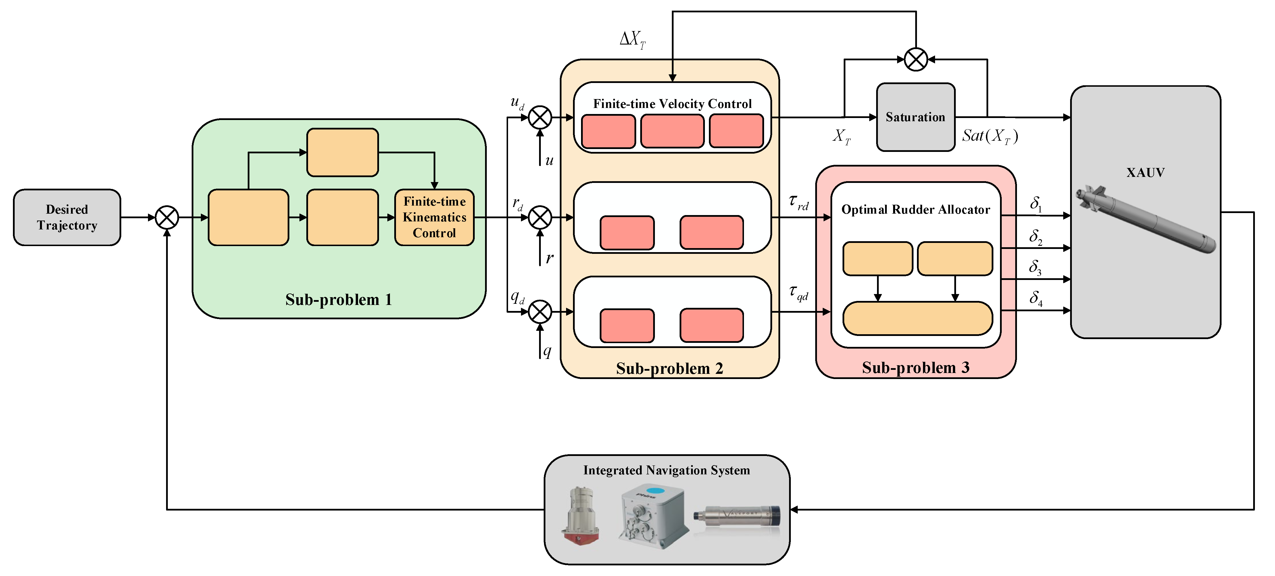
- The finite-time convergence strategy is deeply integrated with the whole controller design process. The novel FTLOS guidance law and finite-time feedback kinematics control law is designed for the kinematics control loop. Improved global finite-time terminal sliding mode control (FTTSMC) laws are proposed for heading control, pitching control, and surge velocity tracking control in the dynamics control loop, where finite time convergence is considered in both the approaching stage and sliding mode holding stage. The FTEDOs are designed to tackle the multi-source unknown uncertainties existing in both the kinematics and dynamics loops. Compared with the existing literature on finite-time control [20,21], this paper not only focuses on the finite convergence of dynamics control, but also proposes a new finite-time convergence guidance algorithm that is easy to implement, making the finite-time control method more comprehensive and effective.
- (2)
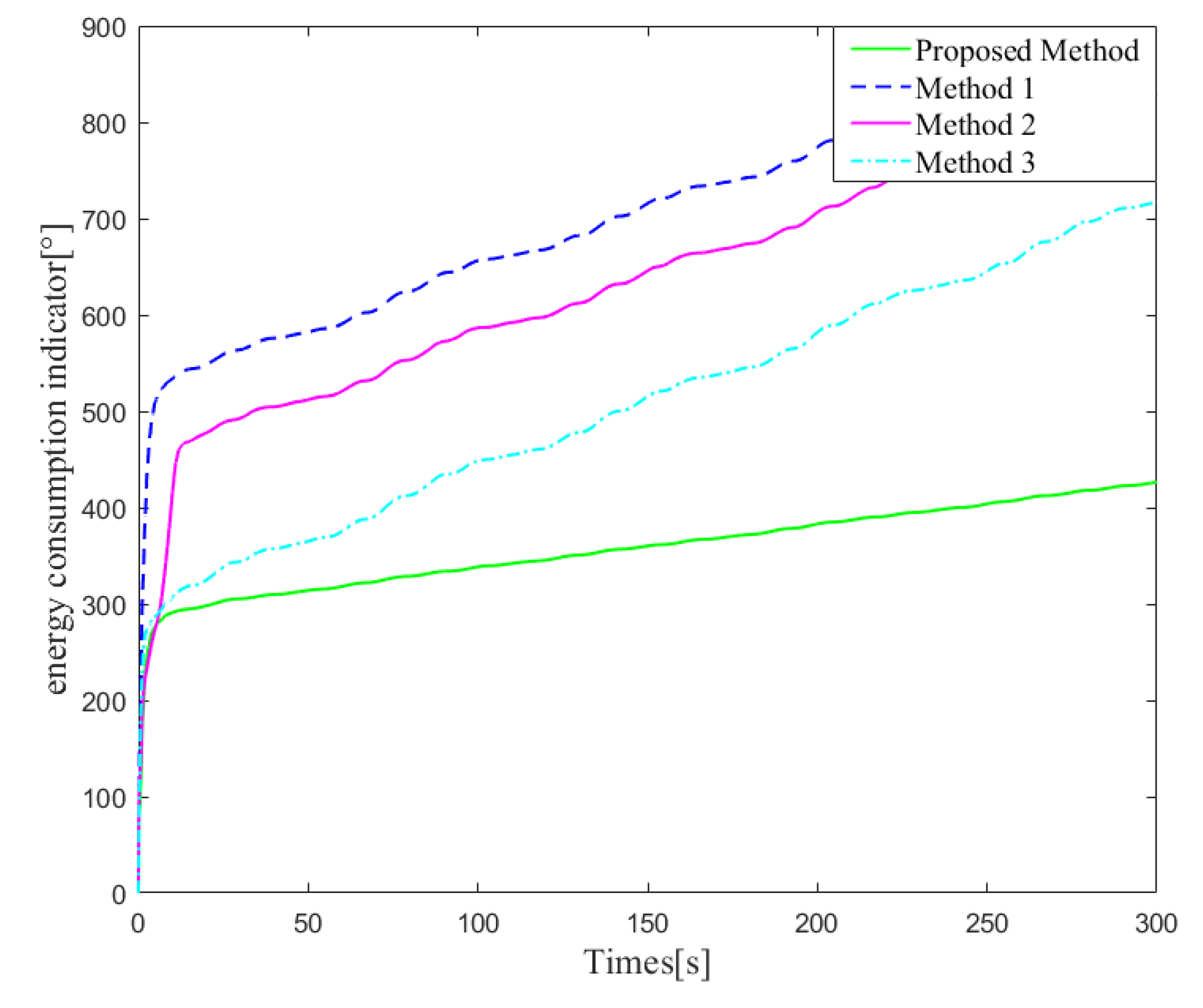
- The influences of actuator dynamics are fully considered, including not only the propeller input saturation problem, but also the complex dynamics mechanism and various constraints of the heterogeneous X-rudder. To deal with the propeller input saturation problem, an adaptive RBFNN compensator is integrated into the surge velocity tracking control law, while for X-rudder dynamics and constraints, a multi-objective optimal rudder allocator is proposed that can realize the rudder angle allocation and energy consumption optimization at the same time, as well as meet the saturation constraints of rudder angle and rudder steering velocity. Compared with the general literatures on actuator characteristics, the research in this paper is more comprehensive.
- (3)
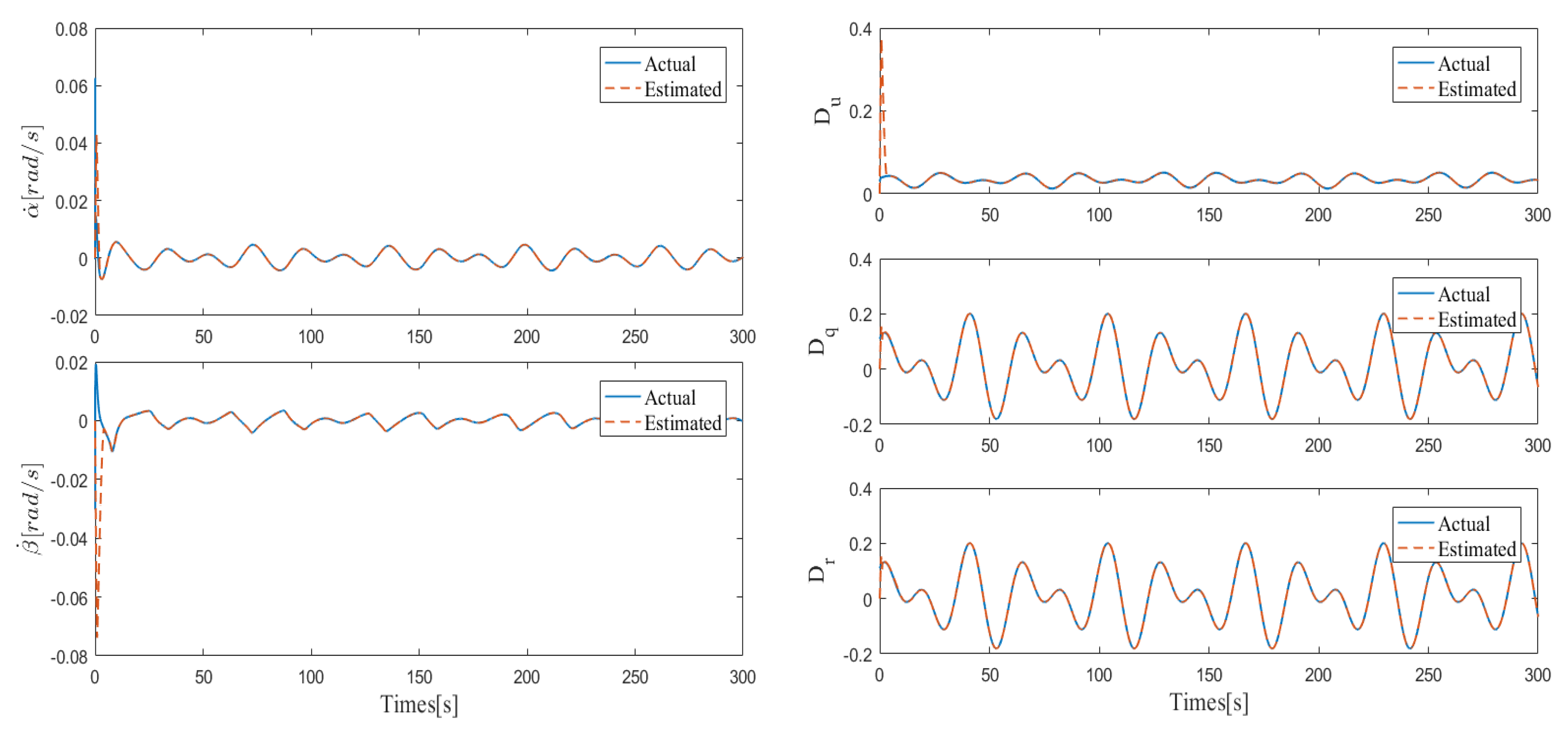
- Multi-source disturbances are considered in both the kinematics model and dynamics model. In particular, and are treated as unknown uncertainties, rather than directly obtained by differential calculation, taking into account the noise problem in the measurement process, which makes the controller design more practical. For the multi-source unknown disturbances, FTEDOs are designed to realize fast and accurate disturbance estimation based on motion state, which greatly improves the robustness of the system. Compared with the conventional disturbance observer, this method can realize the estimation of both the disturbance and its derivative, and shows finite time convergence.
2. XAUV Modeling and Problem Formulation
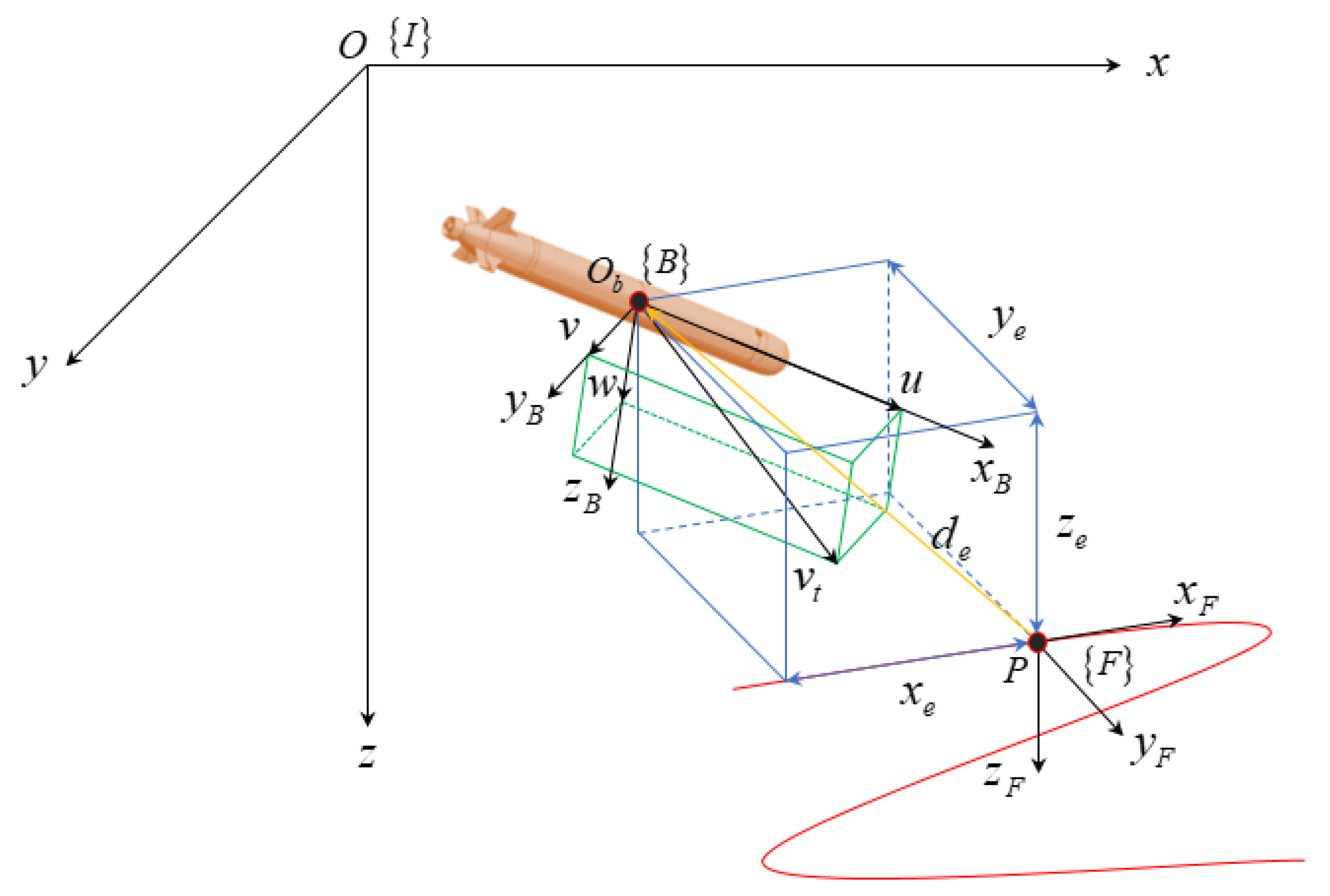
2.1. Preliminaries and Nomenclatures
2.2. XAUV Modeling
2.3. Problem Formulation
2.4. Assumptions
3. Control Methodology
3.1. Finite-Time Extended Disturbance Observer
3.2. Finite-Time Kinematics Control
3.3. Finite-Time Dynamics Control
3.3.1. Finite-Time Heading Control
3.3.2. Finite-Time Pitching Control
3.3.3. Finite-Time Velocity Tracking Control
3.4. Optimal Rudder Allocation
4. Simulation
4.1. Simulation Preparation
- According to the parameter range mentioned above, prepare a group of basic parameters and make the system converge through debugging. In the process of adjustment, adjust the conventional parameters first and then the exponential parameters;
- On the basis of system convergence, the kinematic control parameters are adjusted to improve the convergence speed;
- Further adjust the dynamic control parameters to optimize the tracking control accuracy and convergence speed;
- Adjust the parameters of rudder allocation to optimize the energy consumption.
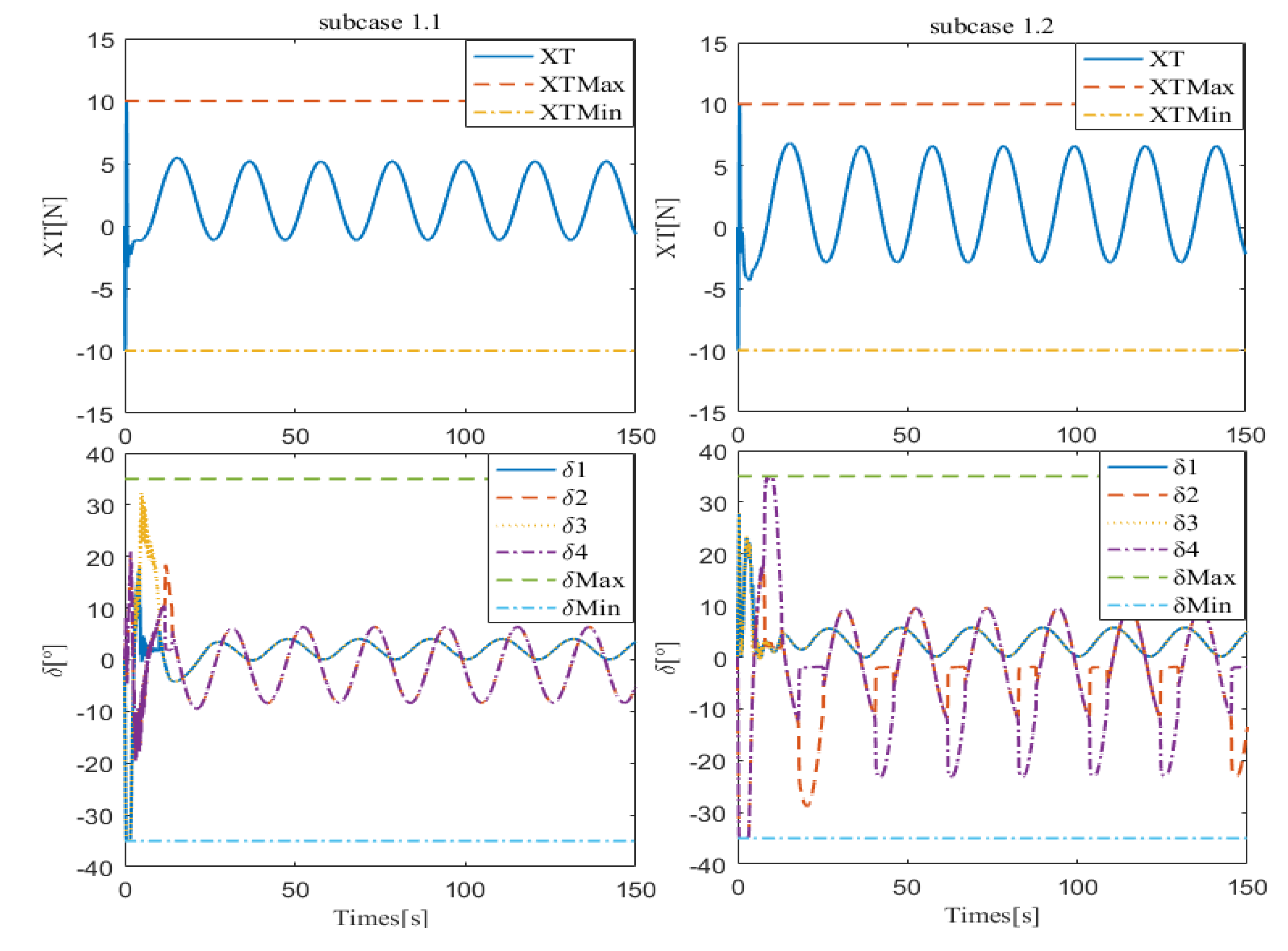
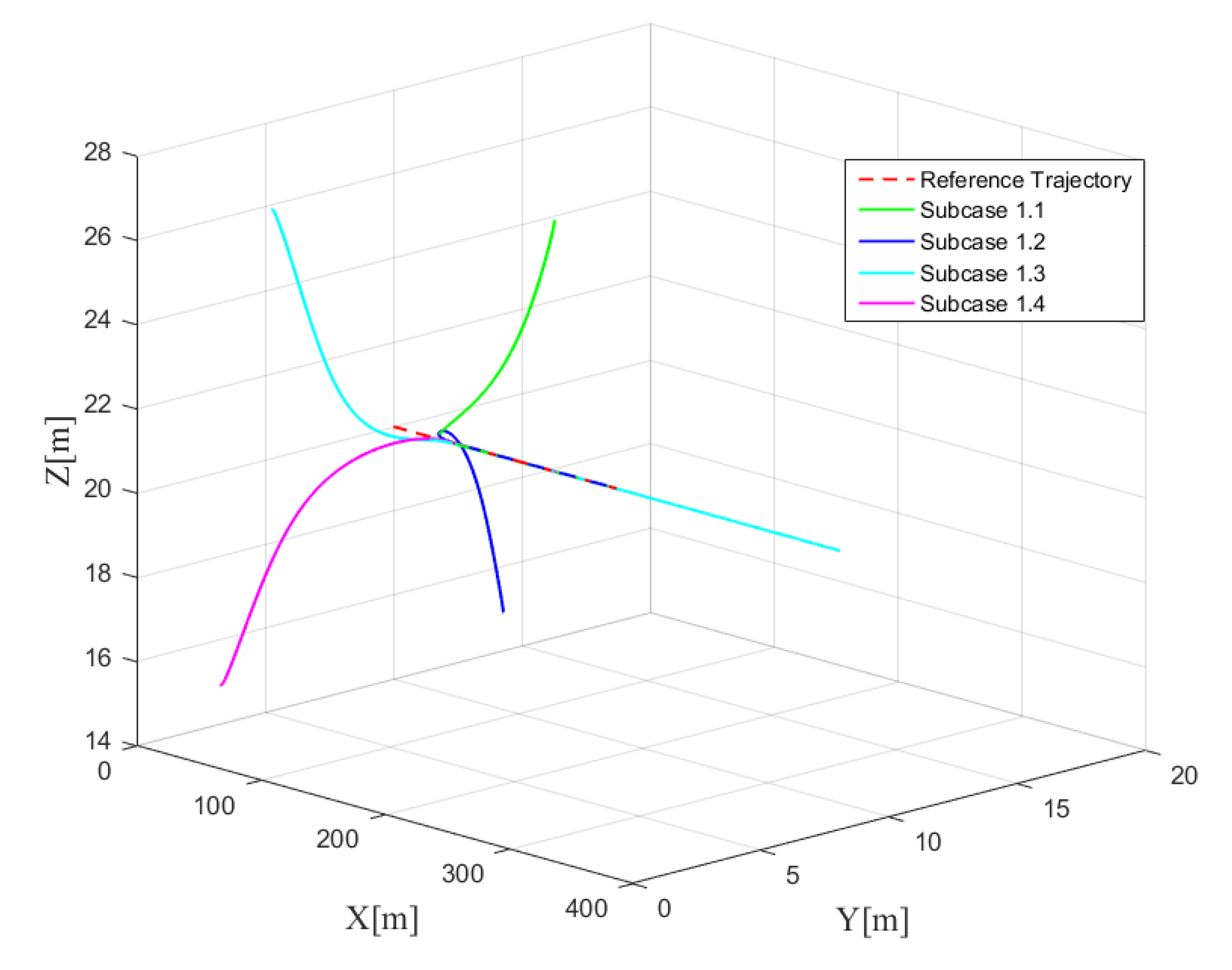
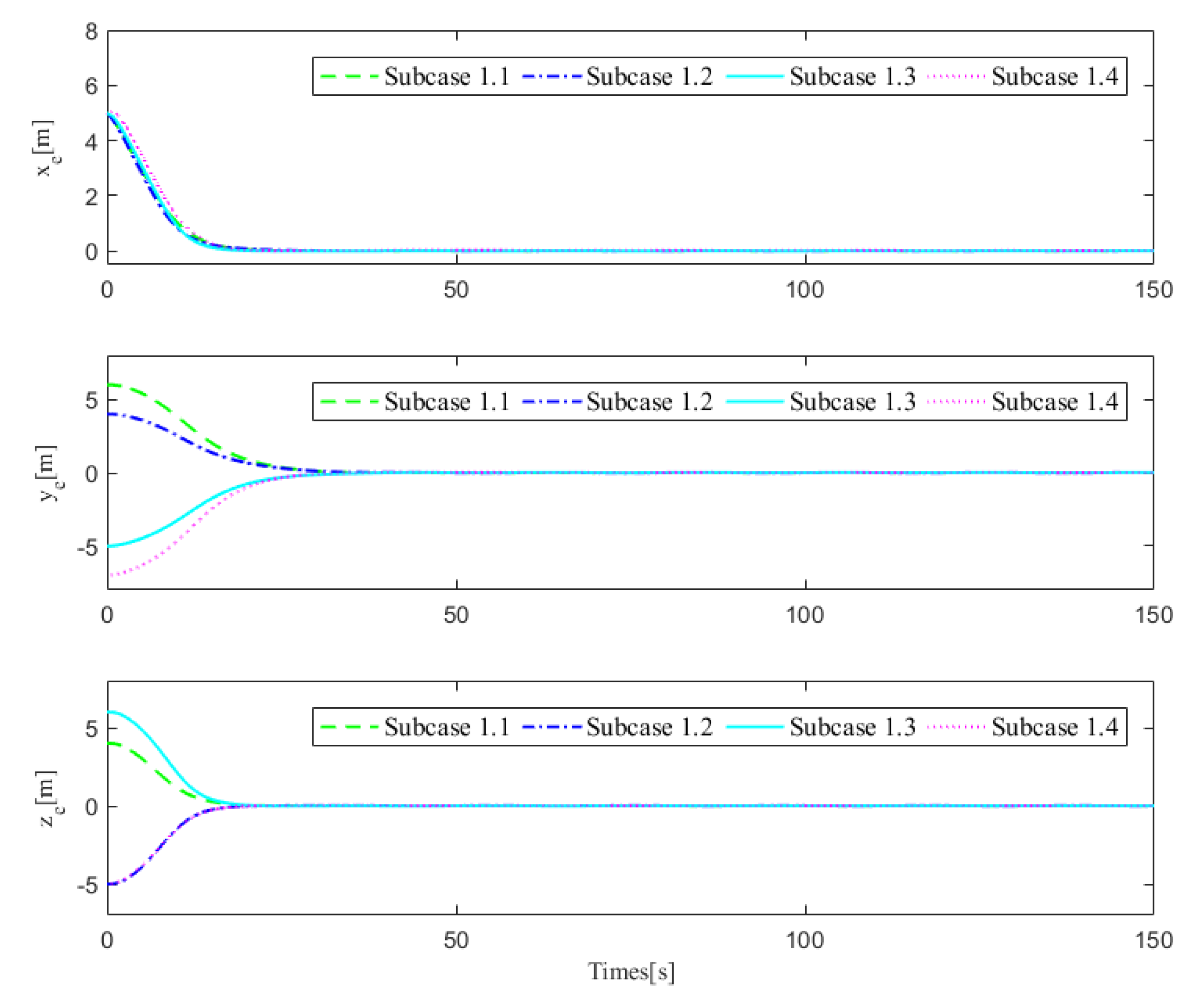
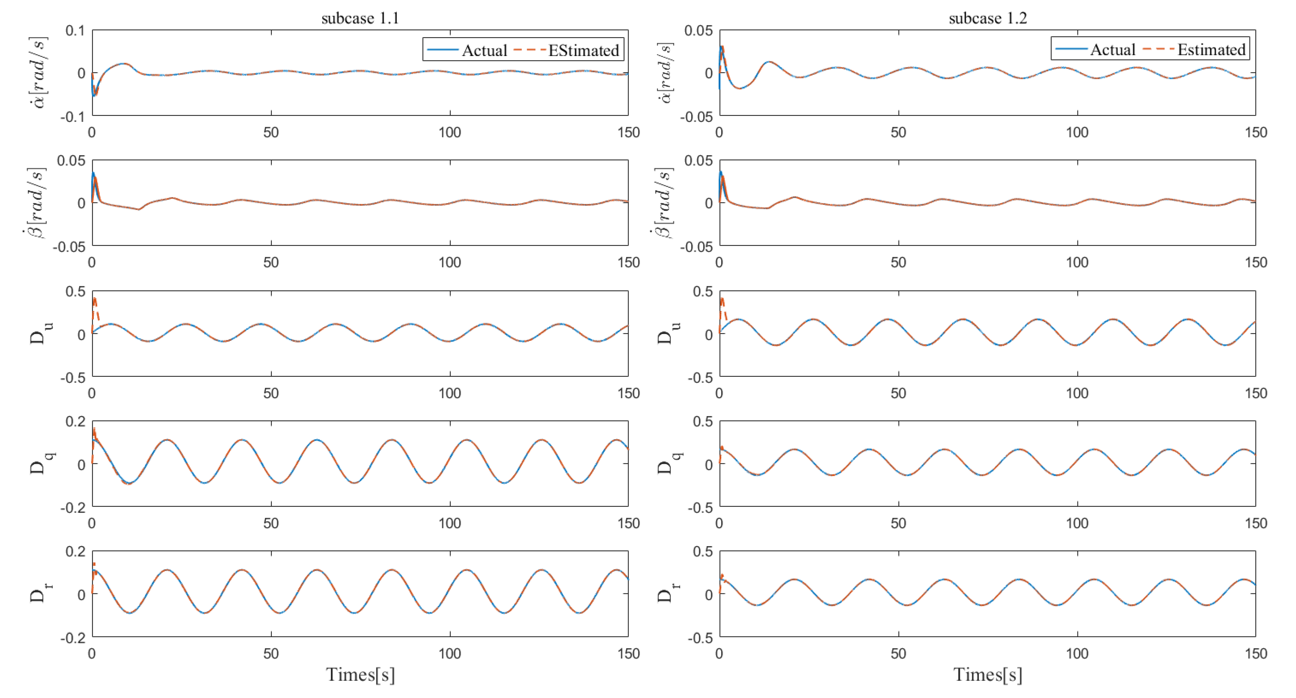
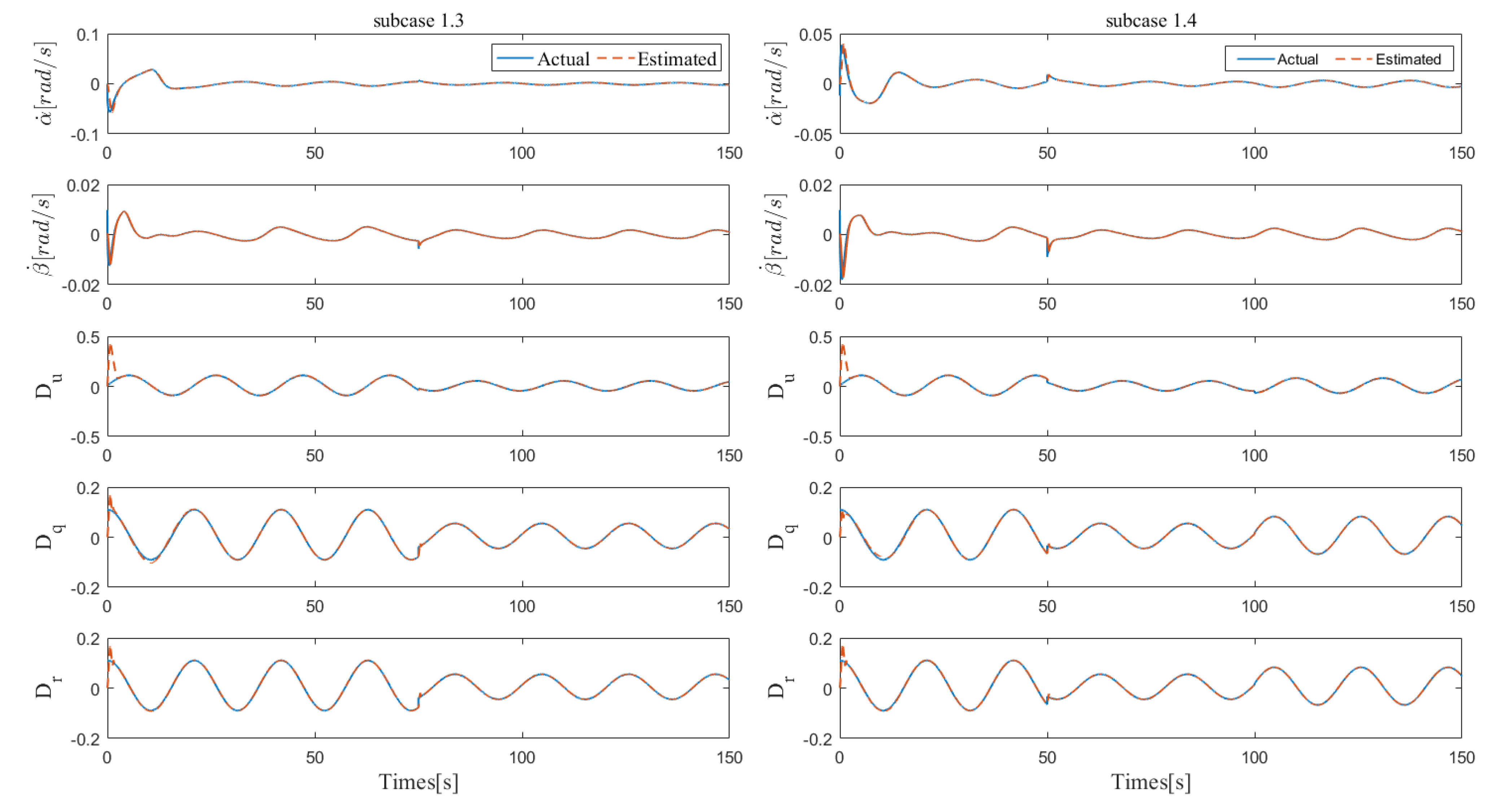
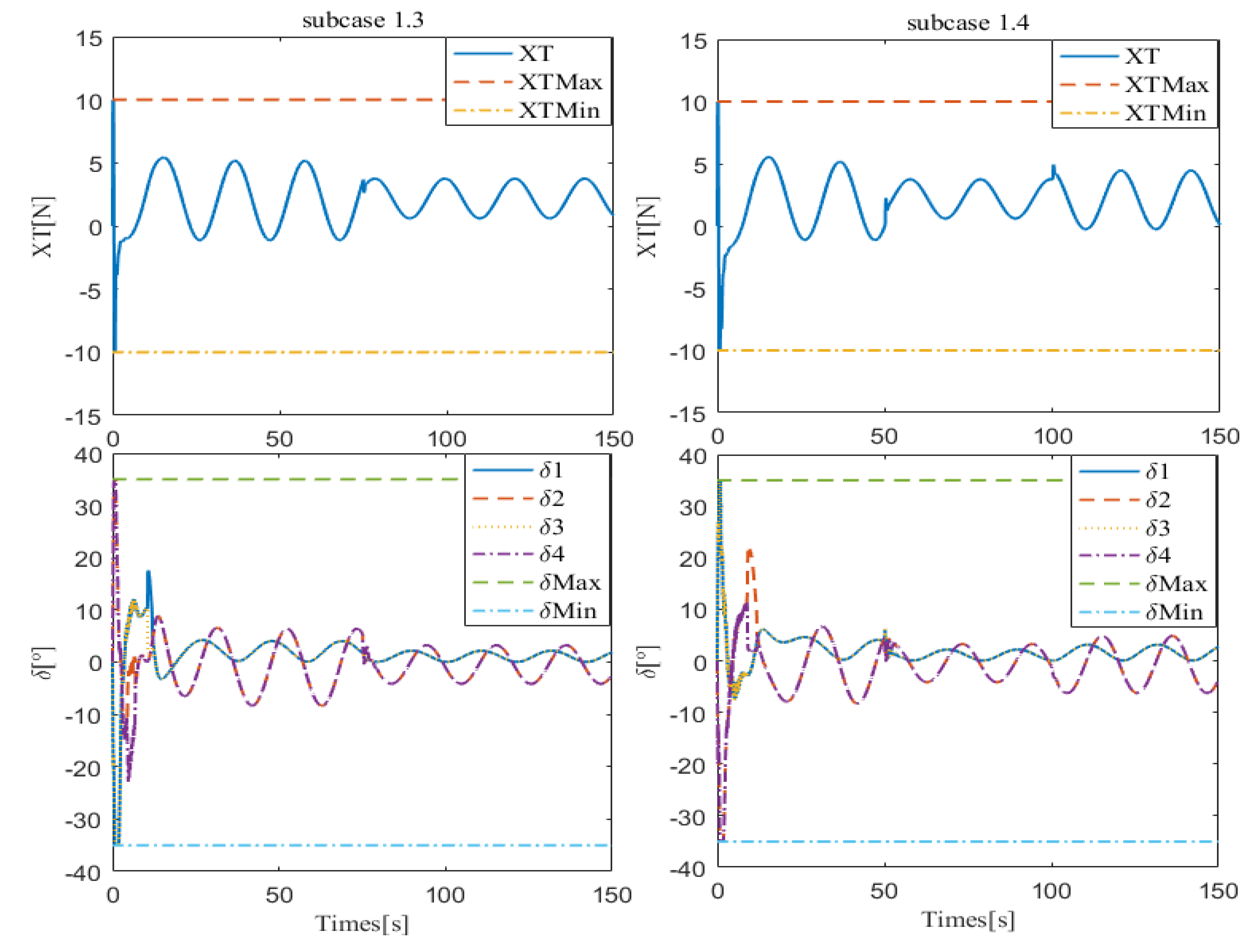
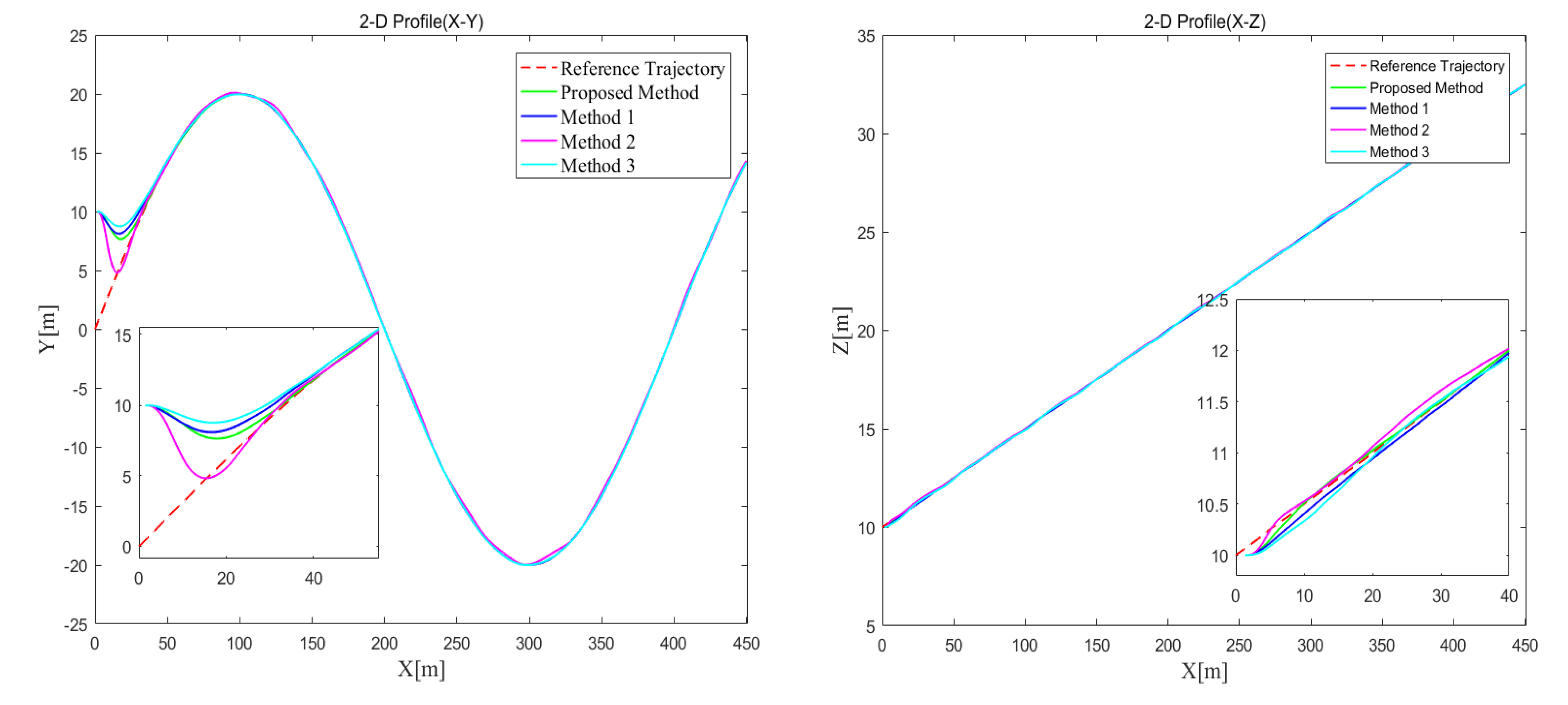
4.2. Case 1
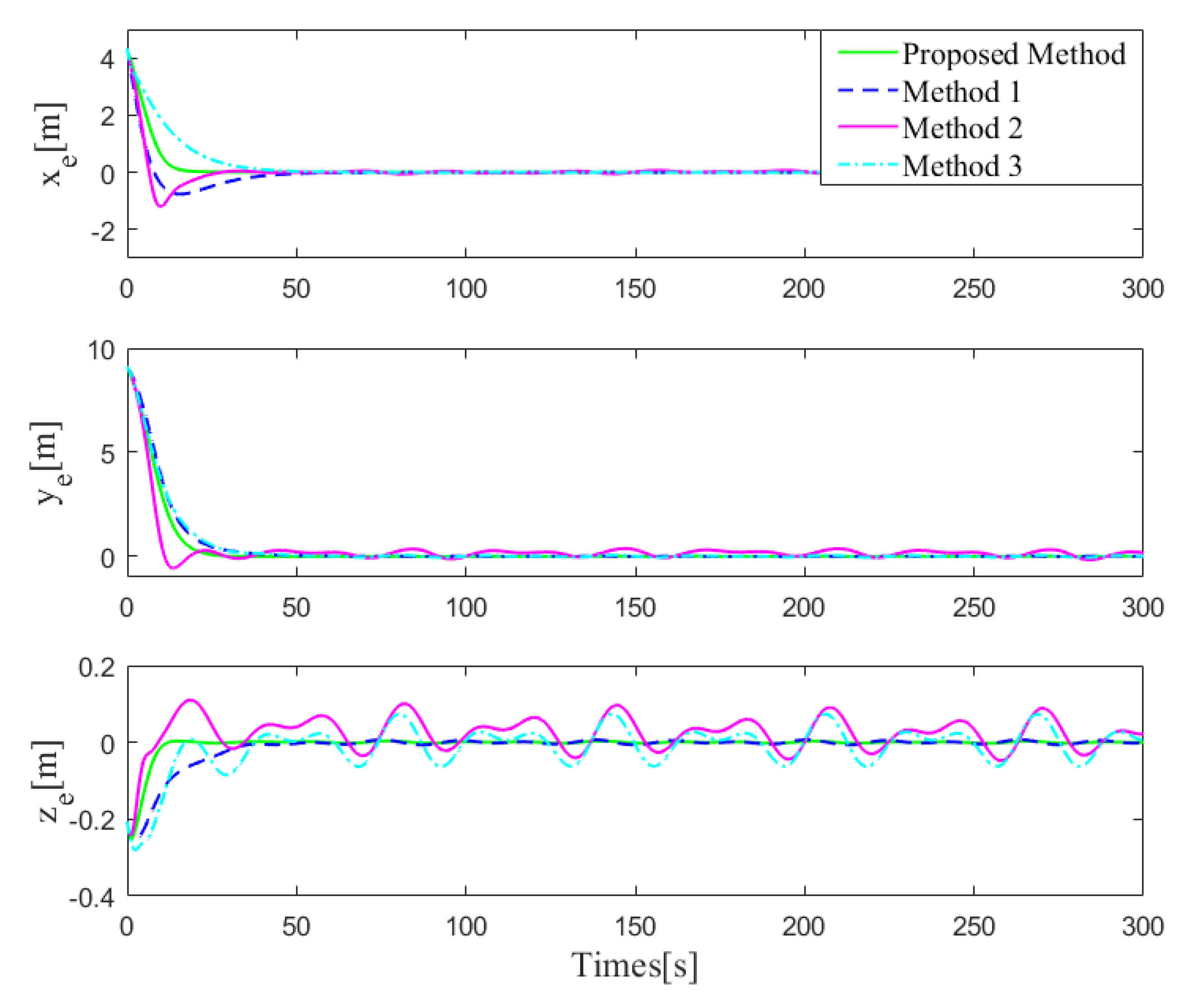
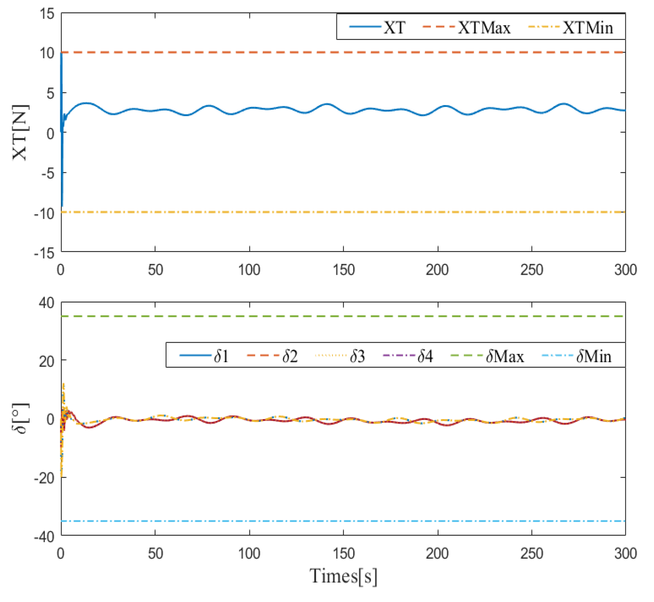
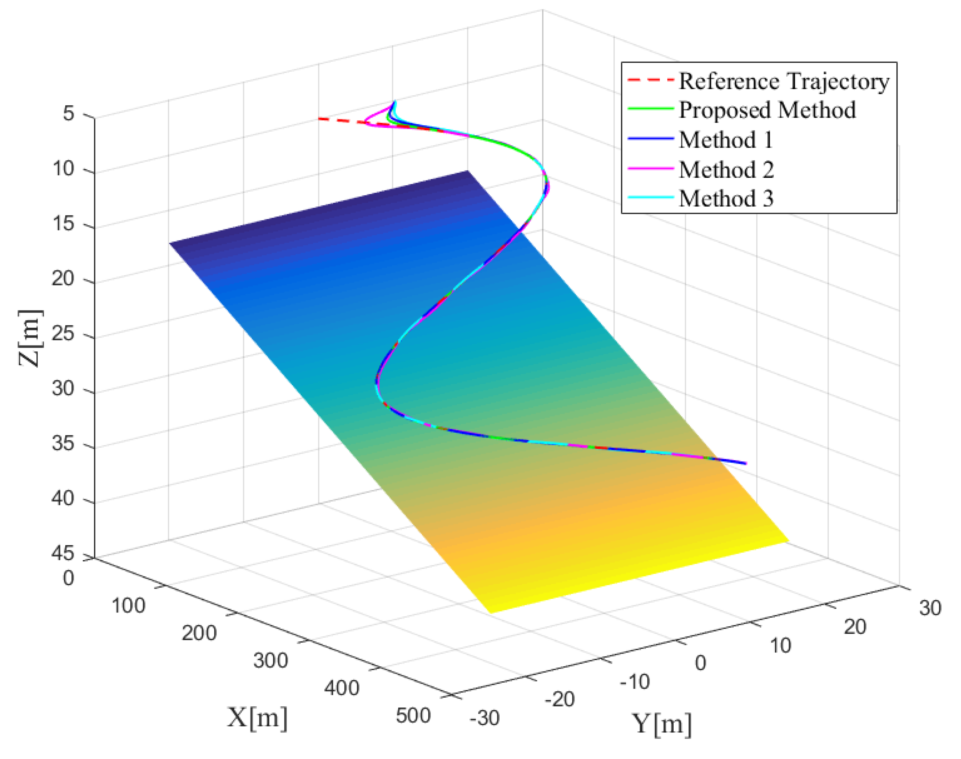
4.3. Case 2
5. Conclusions and Future Works
Author Contributions
Funding
Institutional Review Board Statement
Informed Consent Statement
Data Availability Statement
Conflicts of Interest
Appendix A

| Parameters | Expressions |
|---|---|
References
- Jeon, M.; Yoon, H.K.; Park, J.; You, Y. Analysis of maneuverability of X-rudder submarine considering environmental disturbance and jamming situations. Appl. Ocean Res. 2022, 121, 103079. [Google Scholar] [CrossRef]
- Miller, L.; Brizzolara, S.; Stilwell, D.J. Increase in Stability of an X-Configured AUV through Hydrodynamic Design Iterations with the Definition of a New Stability Index to Include Effect of Gravity. J. Mar. Sci. Eng. 2021, 9, 942. [Google Scholar] [CrossRef]
- Zhang, Y.H.; Li, Y.M.; Sun, Y.S.; Zeng, J.F.; Wan, L. Design and simulation of X rudder AUV’s motion control. Ocean. Eng. 2017, 137, 204–214. [Google Scholar] [CrossRef]
- Xia, Y.; Xu, K.; Huang, Z.; Wang, W.; Xu, G.; Li, Y. Adaptive energy-efficient tracking control of a X rudder AUV with actuator dynamics and rolling restriction. Appl. Ocean Res. 2022, 118, 10299. [Google Scholar] [CrossRef]
- Abdurahman, B.; Savvaris, A.; Tsourdos, A. Switching LOS guidance with speed allocation and vertical course control for path-following of unmanned underwater vehicles under ocean current disturbances. Ocean Eng. 2019, 182, 412–426. [Google Scholar] [CrossRef]
- Mu, D.D.; Wang, G.F.; Fan, Y.S.; Bai, Y.M.; Zhao, Y.S. Fuzzy-Based Optimal Adaptive Line-of-Sight Path Following for Underactuated Unmanned Surface Vehicle with Uncertainties and Time-Varying Disturbances. Math. Probl. Eng. 2018, 2018, 7512606. [Google Scholar] [CrossRef]
- Zheng, Z.; Sun, L. Path following control for marine surface vessel with uncertainties and input saturation. Neurocomputing 2016, 177, 158–167. [Google Scholar] [CrossRef]
- Guerrero, J.; Torres, J.; Creuze, V.; Chemori, A.; Campos, E. Saturation based nonlinear PID control for underwater vehicles: Design, stability analysis and experiments. Mechatronics 2019, 61, 96–105. [Google Scholar] [CrossRef]
- Borlaug, I.L.G.; Pettersen, K.Y.; Gravdahl, J.T. Comparison of two second-order sliding mode control algorithms for an articulated intervention AUV: Theory and experimental results. Ocean Eng. 2021, 222, 108480. [Google Scholar] [CrossRef]
- Hangil, J.; Kim, M.; Yu, S. Second-order sliding-mode controller for autonomous underwater vehicle in the presence of unknown disturbances. Nonlinear Dynam. 2014, 78, 183–196. [Google Scholar]
- Xiang, X.B.; Yu, C.Y.; Lapierre, L.; Zhang, J.L.; Zhang, Q. Survey on Fuzzy-Logic-Based Guidance and Control of Marine Surface Vehicles and Underwater Vehicles. Int. J. Fuzzy Syst. 2018, 20, 572–586. [Google Scholar] [CrossRef]
- Cervantes, J.; Yu, W.; Salazar, S.; Chairez, I. Takagi–sugeno dynamic neuro-fuzzy controller of uncertain nonlinear systems. IEEE Trans. Fuzzy Syst. 2016, 25, 1601–1615. [Google Scholar] [CrossRef]
- Mohammadi, M.; Arefi, M.M.; Vafamand, N.; Kaynak, O. Control of an AUV with completely unknown dynamics and multi-asymmetric input constraints via off-policy reinforcement learning. Neural Comput. Appl. 2022, 34, 5255–5265. [Google Scholar] [CrossRef]
- Wang, S.M.; Duan, F.; Li, Y.; Xia, Y.K.; Li, Z.S. An improved radial basis function for marine vehicle hull form representation and optimization. Ocean Eng. 2022, 260, 112000. [Google Scholar] [CrossRef]
- Rath, B.N.; Subudhi, B. A robust model predictive path following controller for an autonomous underwater vehicle. Ocean Eng. 2022, 244, 110265. [Google Scholar] [CrossRef]
- Shen, C.; Shi, Y. Distributed implementation of nonlinear model predictive control for AUV trajectory tracking. Automatica 2020, 115, 108863. [Google Scholar] [CrossRef]
- Yukhimets, D.; Filaretov, V. The AUV-Follower Control System Based on the Prediction of the AUV-Leader Movement Using Data from the Onboard Video Camera. J. Mar. Sci. Eng. 2022, 10, 1141. [Google Scholar] [CrossRef]
- González-García, J.; Gómez-Espinosa, A.; García-Valdovinos, L.G.; Salgado-Jiménez, T.; Cuan-Urquizo, E.; Escobedo Cabello, J.A. Experimental Validation of a Model-Free High-Order Sliding Mode Controller with Finite-Time Convergence for Trajectory Tracking of Autonomous Underwater Vehicles. Sensors 2022, 22, 488. [Google Scholar] [CrossRef]
- Zhao, L.; Jia, Y.; Yu, J. Adaptive finite-time bipartite consensus for second-order multi-agent systems with antagonistic interactions. Syst. Control Lett. 2017, 102, 22–31. [Google Scholar] [CrossRef]
- Yu, J.; Zhao, L.; Yu, H.; Lin, C.; Dong, W. Fuzzy Finite-Time Command Filtered Control of Nonlinear Systems with Input Saturation. IEEE Trans. Cybern. 2018, 48, 2378–2387. [Google Scholar] [PubMed]
- Dai, Y.; Yang, C.; Yu, S.; Mao, Y.; Zhao, Y. Finite-Time Trajectory Tracking for Marine Vessel by Nonsingular Backstepping Controller with Unknown External Disturbance. IEEE Access 2019, 7, 165897–165907. [Google Scholar] [CrossRef]
- Elhaki, O.; Shojaei, K. Neural network-based target tracking control of underactuated autonomous underwater vehicles with a prescribed performance. Ocean Eng. 2018, 167, 239–256. [Google Scholar] [CrossRef]
- Ali, N.; Tawiah, I.; Zhang, W.D. Finite-time extended state observer based nonsingular fast terminal sliding mode control of autonomous underwater vehicles. Ocean Eng. 2020, 218, 108179. [Google Scholar] [CrossRef]
- Shojaei, K. Neural network feedback linearization target tracking control of underactuated autonomous underwater vehicles with a guaranteed performance. Ocean Eng. 2022, 258, 111827. [Google Scholar] [CrossRef]
- Chu, Z.Z.; Zhu, D.Q.; Jan, G.E. Observer-based adaptive neural network control for a class of remotely operated vehicles. Ocean Eng. 2016, 127, 82–89. [Google Scholar] [CrossRef]
- Peng, Z.H.; Wang, J. Output-Feedback Path-Following Control of Autonomous Underwater Vehicles Based on an Extended State Observer and Projection Neural Networks. IEEE Trans. Syst. Man Cybern. Syst. 2018, 48, 535–544. [Google Scholar] [CrossRef]
- Peng, Z.; Meng, C.; Liu, L.; Wang, D.; Li, T. PWM-driven model predictive speed control for an unmanned surface vehicle with unknown propeller dynamics based on parameter identification and neural prediction. Neurocomputing 2021, 432, 1–9. [Google Scholar] [CrossRef]
- Cui, R.X.; Yang, C.; Li, Y.; Sharma, S. Adaptive neural network control of AUVs with control input nonlinearities using reinforcement learning. IEEE Trans. Syst. Man Cybern. Syst. 2017, 47, 1019–1029. [Google Scholar] [CrossRef]
- An, L.; Li, Y.; Cao, J.; Jiang, Y.; He, J.; Wu, H. Proximate time optimal for the heading control of underactuated autonomous underwater vehicle with input nonlinearities. Appl. Ocean Res. 2020, 95, 102002. [Google Scholar] [CrossRef]
- Yu, C.; Liu, C.; Lian, L.; Xiang, X.; Zeng, Z. ELOS-based path following control for underactuated surface vehicles with actuator dynamics. Ocean Eng. 2019, 187, 106139. [Google Scholar] [CrossRef]
- Zhang, J.; Xiang, X.; Lapierre, L.; Zhang, Q.; Li, W. Approach-angle-based three-dimensional indirect adaptive fuzzy path following of under-actuated AUV with input saturation. Appl. Ocean Res. 2021, 107, 102486. [Google Scholar] [CrossRef]
- Sedghi, F.; Arefi, M.M.; Abooee, A.; Kaynak, O. Adaptive robust finite-time nonlinear control of a typical autonomous underwater vehicle with saturated inputs and uncertainties. IEEE/ASME Trans. Mechatron. 2020, 26, 2517–2527. [Google Scholar] [CrossRef]
- Chu, Z.Z.; Xiang, X.B.; Zhu, D.Q.; Luo, C.M.; Xie, D. Adaptive Fuzzy Sliding Mode Diving Control for Autonomous Underwater Vehicle with Input Constraint. Int. J. Fuzzy Syst. 2018, 20, 1460–1469. [Google Scholar] [CrossRef]
- Park, J.; Sandberg, I.W. Universal approximation using radial-basis-function networks. Neural Comput. 1991, 3, 246–257. [Google Scholar] [CrossRef]
- Yu, S.; Yu, X.; Shirinzadeh, B. Continuous finite-time control for robotic manipulators with terminal sliding mode. Automatica 2005, 41, 1957–1964. [Google Scholar] [CrossRef]
- Qian, C.; Lin, W. Continuous feedback approach to global strong stabilization of nonlinear systems. IEEE Trans. Autom. Control 2001, 46, 1061–1079. [Google Scholar] [CrossRef]
- Qiao, J.; Zhang, D.; Zhu, Y.; Zhang, P. Disturbance observer-based finite-time attitude maneuver control for micro satellite under actuator deviation fault. Aerosp. Sci. Technol. 2018, 82, 262–271. [Google Scholar] [CrossRef]
- Shtessel, Y.; Shkolnikov, I.; Levant, A. Guidance and control of missile interceptor using second-order sliding modes. IEEE Trans. Aerosp. Electron. Syst. 2009, 45, 110–124. [Google Scholar] [CrossRef]
- Van, M. An enhanced tracking control of marine surface vessels based on adaptive integral sliding mode control and disturbance observer. ISA Trans. 2019, 90, 30–40. [Google Scholar] [CrossRef] [PubMed]
- Yu, C.; Liu, C.; Lian, L.; Xiang, X.; Zeng, Z. Onboard system of hybrid underwater robotic vehicles: Integrated software architecture and control algorithm. Ocean Eng. 2019, 187, 106121. [Google Scholar] [CrossRef]
- Miao, J.; Wang, S.; Zhao, Z.; Li, Y.; Tomovic, M.M. Spatial curvilinear path following control of underactuated AUV with multiple uncertainties. ISA Trans. 2017, 67, 107–130. [Google Scholar] [CrossRef] [PubMed]
- Wang, W.; Xia, Y.; Chen, Y.; Xu, G.; Chen, Z.; Xu, K. Motion control methods for x-rudder underwater vehicles: Model based sliding mode and non-model based iterative sliding mode. Ocean Eng. 2020, 216, 108054. [Google Scholar] [CrossRef]


| Nomenclature | Definition |
|---|---|
| XAUV | X-rudder autonomous underwater vehicle |
| FTLOS | Finite-time line-of-sight |
| FTEDO | Finite-time extended disturbance observer |
| FTTSMC | Finite-time terminal sliding mode control |
| DOF | Degree of freedom |
| RBFNN | Radial basis function neural network |
| SQP | Sequential quadratic programming |
| {I} | Inertial reference frame |
| {B} | Body-fixed frame |
| {F} | Frenet–Serret frame |
| The position and orientation variables in {I} | |
| The linear and angular velocities in {B} | |
| Desired position and orientation variables in {I} | |
| The tracking error vectors in {F} | |
| The propeller thrust | |
| The X-rudder forces and torques | |
| The X-rudder angles | |
| The proposed FTLOS guidance laws | |
| The kinematics control laws | |
| The desired rudder torques generated by dynamics control |
| Algorithm: Three-dimensional trajectory tracking |
| Given control parameters |
| Procedure: |
| Input: Collect the data from the integrated navigation system; Calculate the reference trajectory . |
| Finite-time kinematics control law: (1) according to Equation (15); (2) according to Equation (13); (3) according to Equation (20); (4) according to Equation (18). |
|
Finite-time dynamics control law: Heading control law: (1) according to Equation (28); (2) utilizing Equation (29); (3) according to Equation (15); (4) utilizing the finite-time control law Equation (31). Pitching control law: (1) according to Equation (39); (2) utilizing Equation (39); (3) according to Equation (15); (4) utilizing the finite-time control law Equation (41). Velocity tracking control law: (1) according to Equation (43); (2) utilizing Equation (43); (3) according to Equation (15); (4) according to Equation (47); (5) utilizing Equation (46); (6) utilizing the finite-time control law Equation (45). |
| Optimal rudder allocation: (1) according to Equation (49); (2) utilizing Equation (48). |
| The X-rudder equations Equation (10) update (For simulation) Dynamics equations Equation (9) update (For simulation) Kinematics equations Equation (7) update (For simulation) |
| End procedure |
| Repeat procedure |
| Subcases | Disturbance Settings |
|---|---|
| Subcase 1.1 | |
| Subcase 1.2 | |
| Subcase 1.3 | |
| Subcase 1.4 |
| Subcase 1.1 | Subcase 1.2 | Subcase 1.3 | Subcase 1.4 | |
|---|---|---|---|---|
| 0.0018 | 0.0025 | 0.0012 | 0.2502 | |
| 0.0212 | 0.0492 | 0.0061 | 0.0086 | |
| 0.0001 | 0.0003 | |||
| 0.0085 | 0.0195 | 0.0070 | 0.0064 | |
| Name | Method |
|---|---|
| Proposed method | The control method proposed in Section 3 |
| Method 1 | LOS + ISMC [39]: (1) Kinematics control: LOS guidance law; (2) Dynamics control: integral terminal sliding mode controller; (3) Rudder allocation: pseudo inverse method. |
| Method 2 | LOS + FPID [40]: (1) Kinematics control: LOS guidance law; (2) Dynamics control: Fuzzy PID method; (3) Rudder allocation: pseudo inverse method. |
| Method 3 | LOS + Backstepping [41]: (1) Kinematics control: LOS guidance law; (2) Dynamics control: Backstepping method; (3) Rudder allocation: pseudo inverse method. |
| Proposed | Method 1 | Method 2 | Method 3 | |
|---|---|---|---|---|
| 0.0017 | 0.0021 | 0.2725 | 0.0020 | |
| 0.0010 | ||||
| 0.0034 | 0.0035 | 0.1655 | 0.0254 | |
| 0.0168 | 0.0009 | |||
| 0.0014 | 0.0031 | 0.0379 | 0.0316 | |
| 0.0014 | 0.0014 |
Publisher’s Note: MDPI stays neutral with regard to jurisdictional claims in published maps and institutional affiliations. |
© 2022 by the authors. Licensee MDPI, Basel, Switzerland. This article is an open access article distributed under the terms and conditions of the Creative Commons Attribution (CC BY) license (https://creativecommons.org/licenses/by/4.0/).
Share and Cite
Xia, Y.; Huang, Z.; Xu, K.; Xu, G.; Li, Y. Three-Dimensional Trajectory Tracking for a Heterogeneous XAUV via Finite-Time Robust Nonlinear Control and Optimal Rudder Allocation. J. Mar. Sci. Eng. 2022, 10, 1297. https://doi.org/10.3390/jmse10091297
Xia Y, Huang Z, Xu K, Xu G, Li Y. Three-Dimensional Trajectory Tracking for a Heterogeneous XAUV via Finite-Time Robust Nonlinear Control and Optimal Rudder Allocation. Journal of Marine Science and Engineering. 2022; 10(9):1297. https://doi.org/10.3390/jmse10091297
Chicago/Turabian StyleXia, Yingkai, Zhemin Huang, Kan Xu, Guohua Xu, and Ye Li. 2022. "Three-Dimensional Trajectory Tracking for a Heterogeneous XAUV via Finite-Time Robust Nonlinear Control and Optimal Rudder Allocation" Journal of Marine Science and Engineering 10, no. 9: 1297. https://doi.org/10.3390/jmse10091297
APA StyleXia, Y., Huang, Z., Xu, K., Xu, G., & Li, Y. (2022). Three-Dimensional Trajectory Tracking for a Heterogeneous XAUV via Finite-Time Robust Nonlinear Control and Optimal Rudder Allocation. Journal of Marine Science and Engineering, 10(9), 1297. https://doi.org/10.3390/jmse10091297