
Numerical Analysis of an Overtopping Wave Energy Converter Subjected to the Incidence of Irregular and Regular Waves from Realistic Sea States


 , , , ,
 ,
,  and
and 
Abstract
1. Introduction
2. Ocean Wave Energy and Its Conversion
3. Data and Methodology
3.1. Mathematical and Numerical Modeling
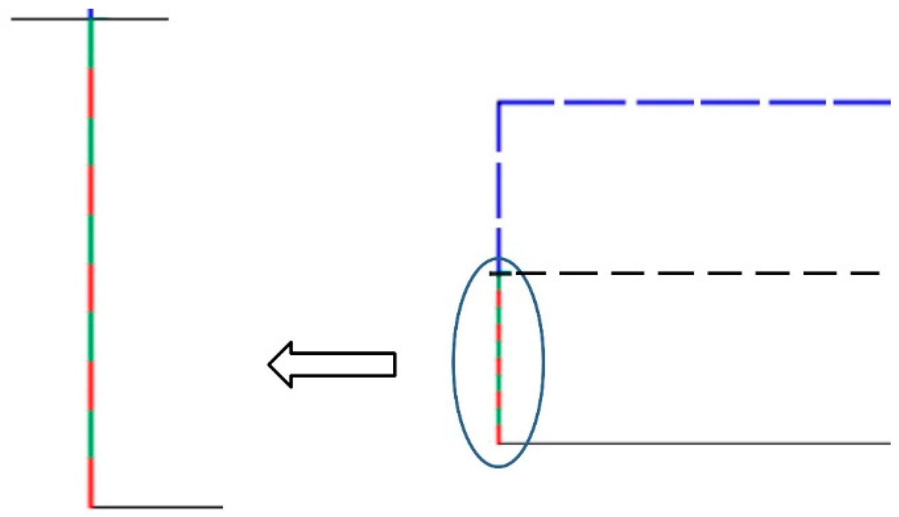
Realistic Sea State Data and Wave Generation
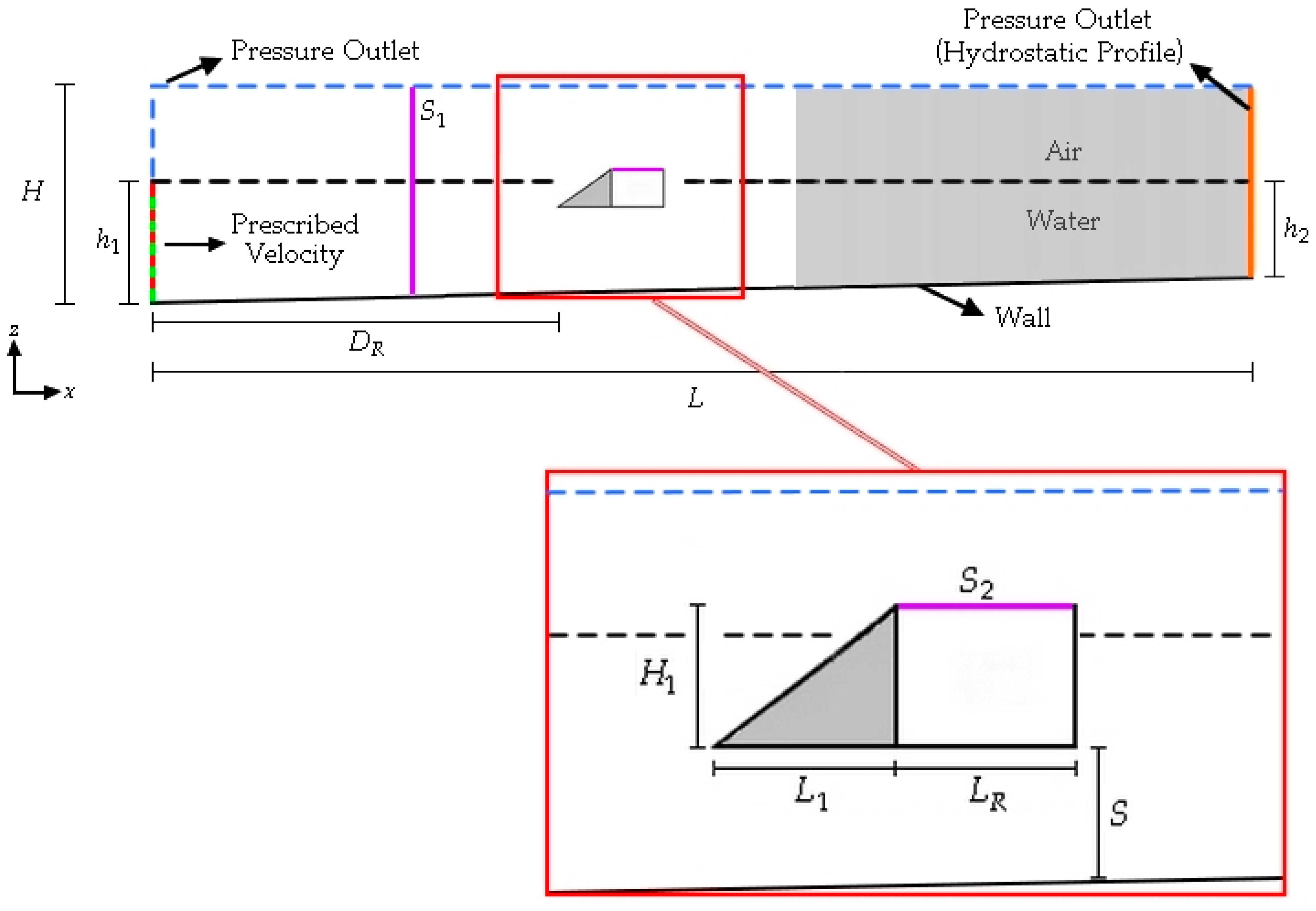
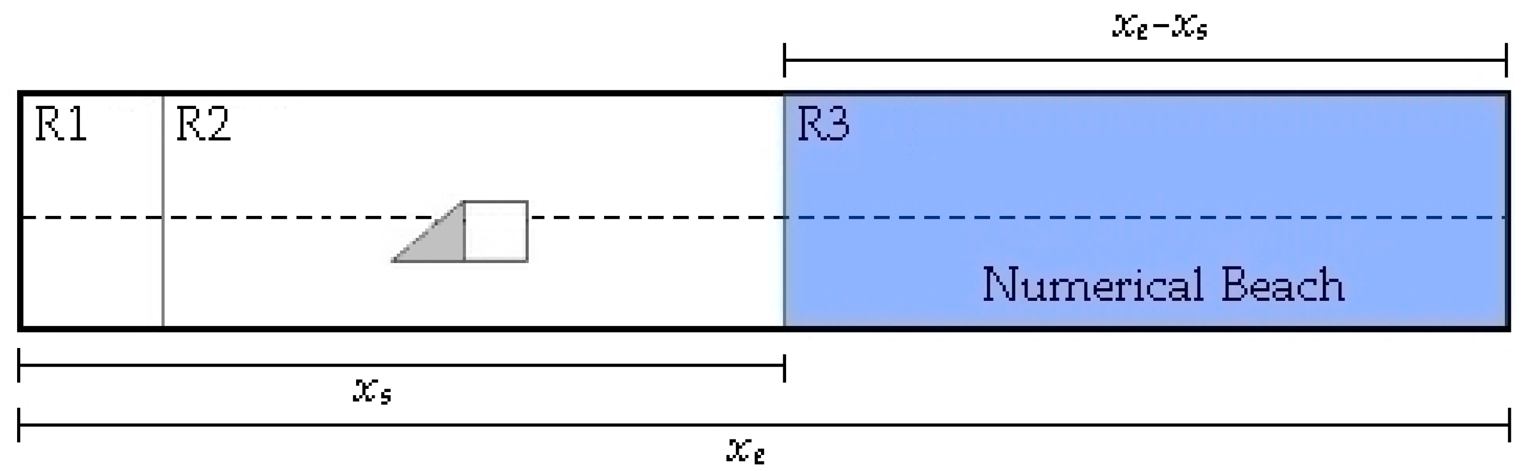
3.2. Problem Description
4. Results
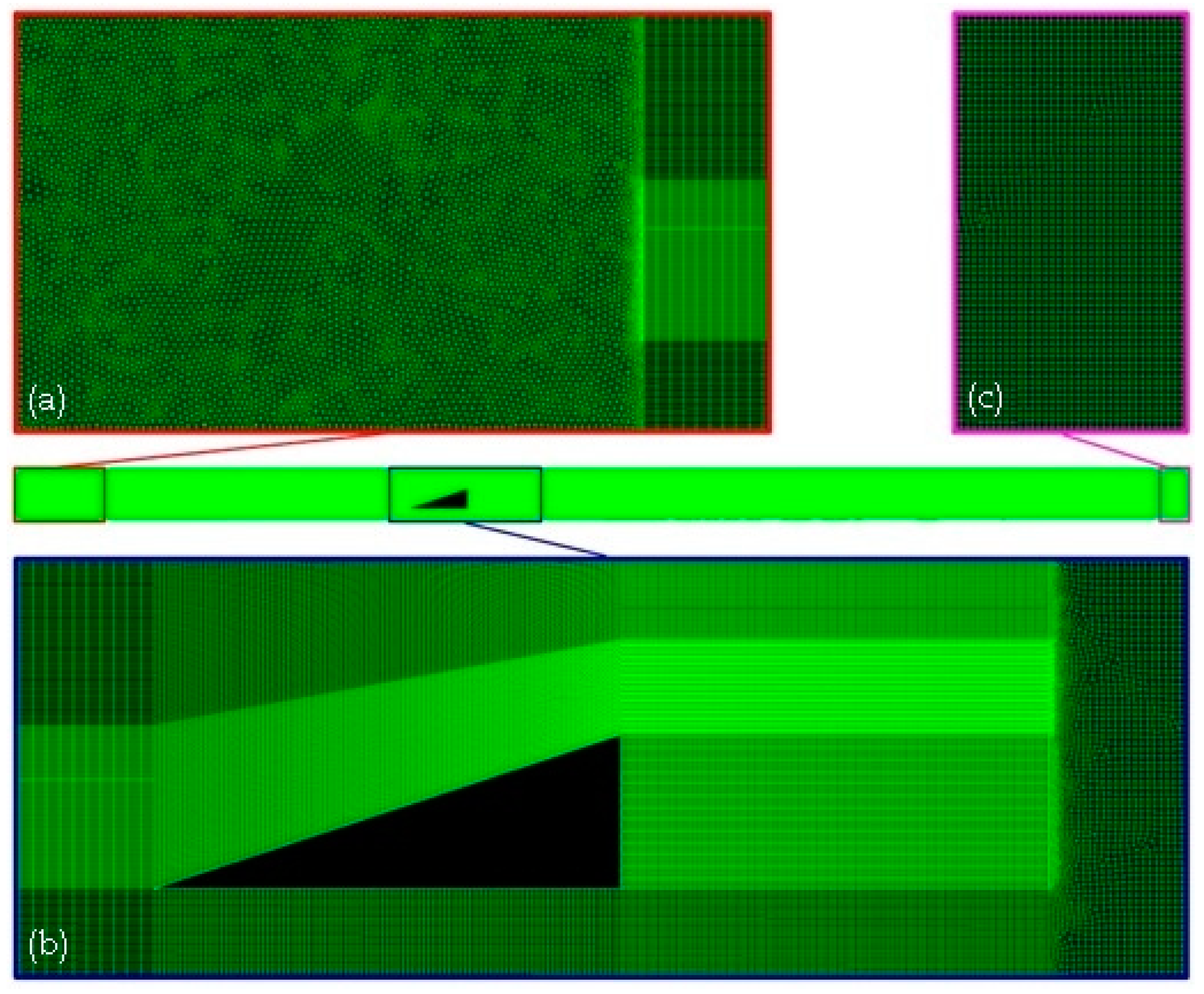
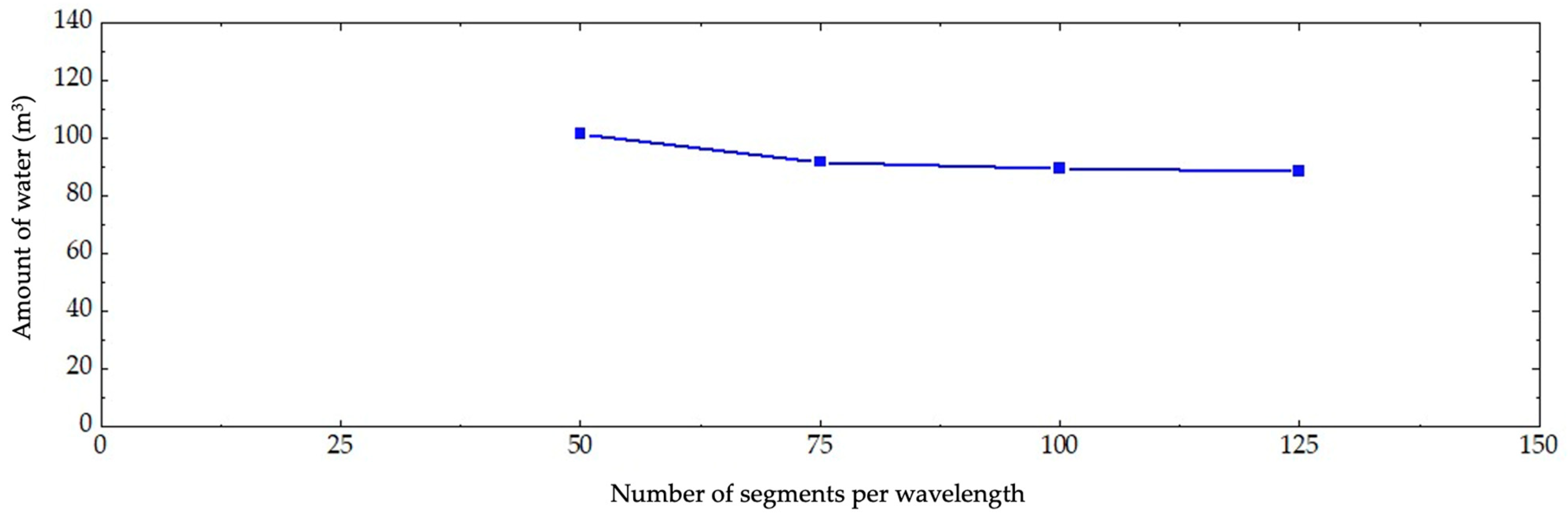
4.1. Mesh Independence Test
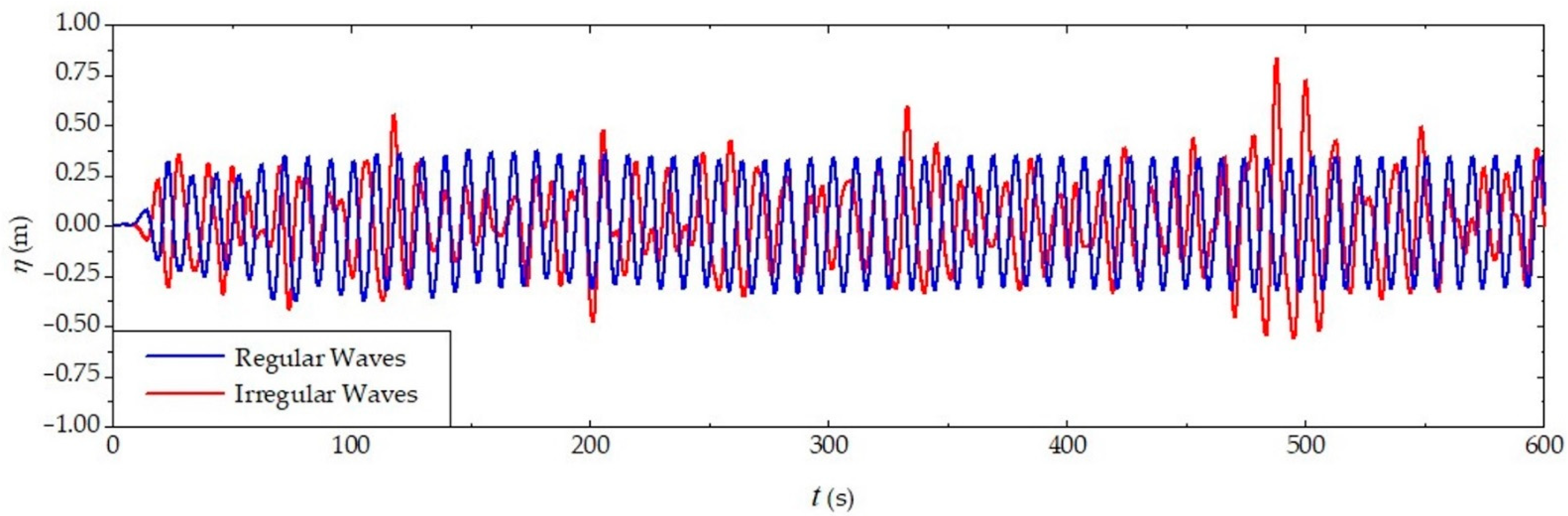
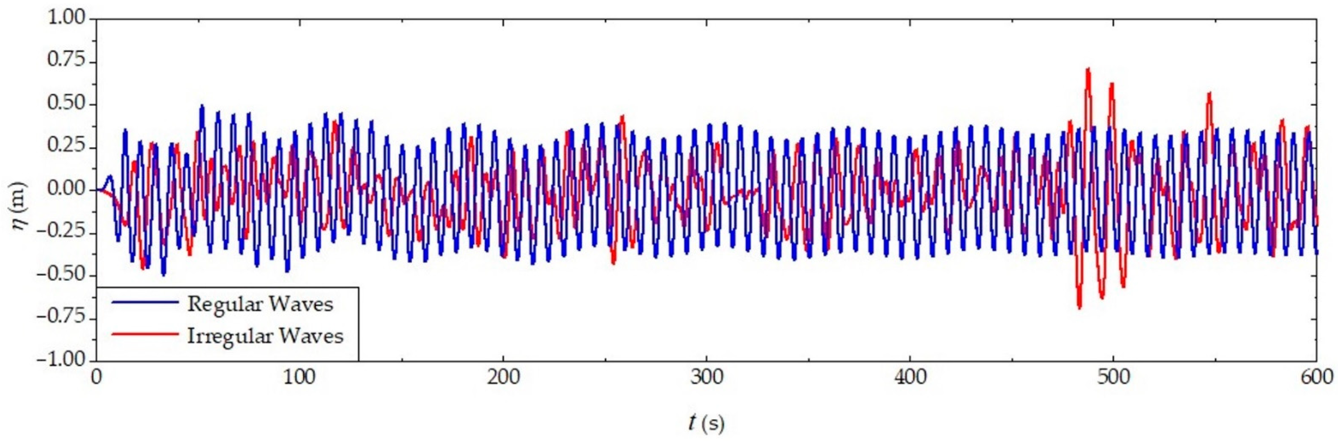
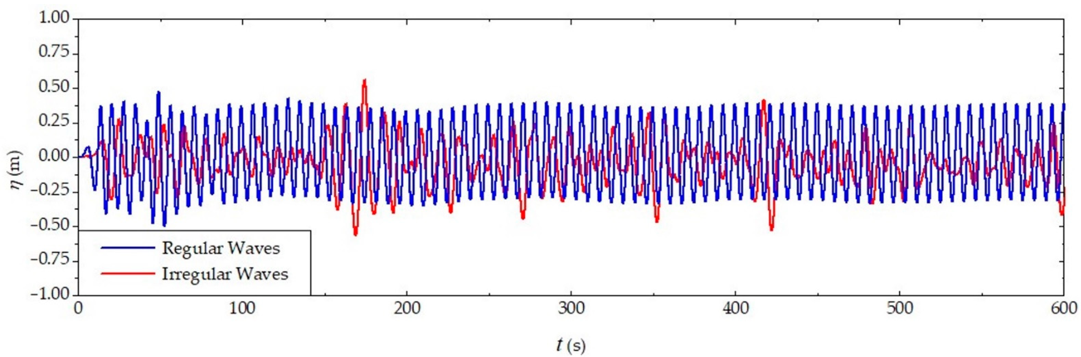
4.2. Incidence of Waves on the Overtopping WEC
5. Conclusions
Author Contributions
Funding
Institutional Review Board Statement
Informed Consent Statement
Data Availability Statement
Acknowledgments
Conflicts of Interest
References
- Fontana, R.L.M.; Costa, S.S.; Silva, J.A.B.; Rodrigues, A.J. Teorias Demográficas e o Crescimento Populacional no Mundo. Cadernos de Graduação. Ciências Hum. E Sociais Unit 2015, 2, 113–124. [Google Scholar]
- REN21. Renewables 2019: Global Status Report; REN21: Paris, France, 2019. [Google Scholar]
- Gunn, K.; Stock-Williams, C. Quantifying the global wave power resource. Renew. Energy 2012, 44, 296–304. [Google Scholar] [CrossRef]
- Espindola, R.L.; Araújo, A.M. Wave energy resource of Brazil: An analysis from 35 years of ERA—Interim reanalysis data. PLoS ONE 2017, 12, e0183501. [Google Scholar] [CrossRef] [PubMed]
- Pecher, A.; Kofoed, J.P. Handbook of Ocean Wave Energy; Springer: Cham, Switzerland, 2017. [Google Scholar]
- Jungrungruengtaworn, S.; Hyun, B.-S. Influence of Slot Width on the Performance of Multi-Stage Overtopping Wave Energy Converters. Int. J. Nav. Archit. Ocean Eng. 2017, 9, 668–676. [Google Scholar] [CrossRef]
- Han, Z.; Liu, Z.; Shi, H. Numerical study on overtopping performance of a multi-level breakwater for wave energy conversion. Ocean Eng. 2018, 150, 94–101. [Google Scholar] [CrossRef]
- Liu, Z.; Han, Z.; Shi, H.; Yang, W. Experimental study on multi-level overtopping wave energy convertor under regular wave conditions. Int. J. Nav. Archit. Ocean Eng. 2018, 10, 651–659. [Google Scholar] [CrossRef]
- Martins, J.C.; Goulart, M.M.; das Gomes, M.N.; Souza, J.A.; Rocha, L.A.O.; Isoldi, L.A.; Dos Santos, E.D. Geometric evaluation of the main operational principle of an overtopping wave energy converter by means of Constructal Design. Renew. Energy 2018, 118, 727–741. [Google Scholar] [CrossRef]
- Palma, G.; Formentin, S.M.; Zanuttigh, B.; Contestabile, P.; Vicinanza, D. Numerical Simulations of the Hydraulic Performance of a Breakwater-Integrated Overtopping Wave Energy Converter. J. Mar. Sci. Eng. 2019, 7, 38. [Google Scholar] [CrossRef]
- Di Lauro, E.; Lara, J.L.; Maza, M.; Losada, I.J.; Contestabile, P.; Vicinanza, D. Stability analysis of a non-conventional breakwater for wave energy conversion. Coast. Eng. 2019, 145, 36–52. [Google Scholar] [CrossRef]
- Di Lauro, E.; Maza, M.; Lara, J.L.; Losada, I.J.; Contestabile, P.; Vicinanza, D. Advantages of an innovative vertical breakwater with an overtopping wave energy converter. Coast. Eng. 2020, 159, 103713. [Google Scholar] [CrossRef]
- Martins, J.C.; Fragassa, C.; Goulart, M.M.; dos Santos, E.D.; Isoldi, L.A.; das Neves Gomes, M.; Rocha, L.A.O. Constructal Design of an Overtopping Wave Energy Converter Incorporated in a Breakwater. J. Mar. Sci. Eng. 2022, 10, 471. [Google Scholar] [CrossRef]
- Liu, Z.; Shi, H.; Cui, Y.; Kim, K. Experimental study on overtopping performance of a circular ramp wave energy converter. Renew. Energy 2017, 104, 163–176. [Google Scholar] [CrossRef]
- Barbosa, D.V.E.; Santos, A.L.G.; Dos Santos, E.D.; Souza, J.A. Overtopping device numerical study: Openfoam solution verification and evaluation of curved ramps performances. Int. J. Heat Mass Transf. 2019, 131, 411–423. [Google Scholar] [CrossRef]
- Contestabile, P.; Crispino, G.; Russo, S.; Gisonni, C.; Cascetta, F.; Vicinanza, D. Crown wall modifications as response to wave overtopping under a future sea level scenario: An experimental parametric study for an innovative composite seawall. Appl. Sci. 2020, 10, 2227. [Google Scholar] [CrossRef]
- Mariani, A.; Crispino, G.; Contestabile, P.; Cascetta, F.; Gisonni, C.; Vicinanza, D.; Unich, A. Optimization of Low Head Axial-Flow Turbines for an Overtopping BReakwater for Energy Conversion: A Case Study. Energies 2021, 14, 4618. [Google Scholar] [CrossRef]
- Machado, B.N.; Oleinik, P.H.; Kirinus, E.P.; Dos Santos, E.D.; Rocha, L.A.O.; Das Gomes, M.N.; Conde, J.M.P.; Isoldi, L.A. WaveMIMO Methodology: Numerical Wave Generation of a Realistic Sea State. J. Appl. Comput. Mech. 2021, 1, 2129–2148. [Google Scholar] [CrossRef]
- Taboada, J.V.; Casás, V.D.; Yu, X.; Gemilang, G.M.; Sampaio, P. Study review of the electrical power generation: Wave energy converting device system from the swell. IOP Conf. Ser. Mater. Sci. Eng. 2021, 1201, 012001. [Google Scholar] [CrossRef]
- Chen, G.; Chapron, B.; Ezraty, R.; Vandemark, D. A Global View of Swell and Wind Sea Climate in the Ocean by Satellite Altimeter and Scatterometer. J. Atmos. Ocean. Technol. 2002, 19, 1849–1859. [Google Scholar] [CrossRef]
- Kharati-Koopaee, M.; Kiali-Kooshkghazi, M. Assessment of plate-length effect on the performance of the horizontal plate wave energy converter. J. Waterw. Port Coast. Ocean Eng. 2019, 145, 04018037. [Google Scholar] [CrossRef]
- Seibt, F.M.; Camargo, F.V.; Dos Santos, E.D.; Neves, G.M.; Rocha, L.A.O.; Isoldi, L.A.; Fragassa, C. Numerical evaluation on the efficiency of the submerged horizontal plate type wave energy converter. FME Trans. 2019, 47, 543–551. [Google Scholar] [CrossRef]
- Chakraborty, T.; Majumder, M. Impact of extreme events on conversion efficiency of wave energy converter. Energy Sci. Eng. 2020, 8, 3441–3456. [Google Scholar] [CrossRef]
- Kralli, V.-E.; Theodossiou, N.; Karambas, T. Optimal Design of Overtopping Breakwater for Energy Conversion (OBREC) Systems Using the Harmony Search Algorithm. Front. Energy Res. 2019, 7, 80. [Google Scholar] [CrossRef]
- Zabihi, M.; Mazaheri, S.; Rezaee Mazyak, A. Wave Generation in a Numerical Wave Tank. Int. J. Coast. Offshore Eng. 2017, 5, 25–35. [Google Scholar]
- Machado, B.N.; Kisner, E.V.; Paiva, M.S.; Gomes, M.N.; Rocha, L.A.O.; Marques, W.C.; Santos, E.D.; Isoldi, L.A. Numerical Generation of Regular Waves Using Discrete Analytical Data as Boundary Condition of Prescribed Velocity. In Proceedings of the XXXVIII Iberian Latin-American Congress on Computational Methods in Engineering, Rio de Janeiro, Brazil, 5–8 November 2017. [Google Scholar]
- Machado, F.M.M.; Lopes, A.M.G.; Ferreira, A.D. Numerical simulation of regular waves: Optimization of a numerical wave tank. Ocean Eng. 2018, 170, 89–99. [Google Scholar] [CrossRef]
- Finnegan, W.; Goggins, J. Linear irregular wave generation in a numerical wave tank. Appl. Ocean Res. 2015, 52, 188–200. [Google Scholar] [CrossRef]
- Higuera, P.; Lara, J.L.; Losada, I.J. Realistic wave generation and active wave absorption for Navier–stokes models. Coast. Eng. 2013, 71, 102–118. [Google Scholar] [CrossRef]
- Higuera, P.; Lara, J.L.; Losada, I.J. Simulating coastal engineering processes with OpenFOAM®. Coast. Eng. 2013, 71, 119–134. [Google Scholar] [CrossRef]
- Patankar, S.V. Numerical Heat Transfer and Fluid Flow; McGraw Hill: New York, NY, USA, 1980. [Google Scholar]
- Versteeg, H.K.; Malalasekera, W. An Introduction to Computational Fluid Dynamics: The Finite Volume Method, 2nd ed.; Pearson Education: London, UK, 2007. [Google Scholar]
- Hirt, C.W.; Nichols, B.D. Volume of Fluid (VOF) Method for the Dynamics of Free Boundaries. J. Comput. Phys. 1981, 39, 201–225. [Google Scholar] [CrossRef]
- Schlichting, H. Boundary Layer Theory, 7th ed.; McGraw-Hill: New York, NY, USA, 1979. [Google Scholar]
- Foyhirun, C.; Kositgittiwong, D.; Ekkawatpanit, C. Wave energy potential and simulation on the Andaman sea coast of Thailand. Sustainability 2020, 12, 3657. [Google Scholar] [CrossRef]
- Lisboa, R.C.; Teixeira, P.R.; Didier, E. Regular and irregular wave propagation analysis in a flume with numerical beach using a Navier-stokes based model. Defect Diffus. Forum 2017, 372, 81–90. [Google Scholar] [CrossRef]
- Awk, T. TOMAWAC User Manual Version 7.2. 7.2.3; The Telemac-Mascaret Consortium: Chatou, France, 2017. [Google Scholar]
- Maciel, R.P.; Fragassa, C.; Machado, B.N.; Rocha, L.A.O.; Dos Santos, E.D.; Das Gomes, M.N.; Isoldi, L.A. Verification and Validation of a Methodology to Numerically Generate Waves Using Transient Discrete Data as Prescribed Velocity Boundary Condition. J. Mar. Sci. Eng. 2021, 9, 896. [Google Scholar] [CrossRef]
- Oleinik, P.H.; Tavares, G.P.; Machado, B.N.; Isoldi, L.A. Transformation of water wave spectra into time series of surface elevation. Earth 2021, 2, 997–1005. [Google Scholar] [CrossRef]
- Airy, G.B. Tides and Waves; Encyclopædia Metropolitana: London, UK, 1845. [Google Scholar]
- Dean, R.G.; Dalrymple, R.A. Water Wave Mechanics for Engineers and Scientists; World Scientific: Singapore, 1991; Volume 2. [Google Scholar]
- Chakrabarti, S.K. Handbook of Offshore Engineering; Elsevier: Chicago, IL, USA, 2005. [Google Scholar]
- Liu, Z.; Hyun, B.S.; Hong, K. Numerical study of air chamber for oscillating water column wave energy converter. China Ocean Eng. 2011, 25, 169–178. [Google Scholar] [CrossRef]
- Gomes, M.; Das, N.; Lorenzini, G.; Rocha, L.A.O.; Dos Santos, E.D.; Isoldi, L.A. Constructal Design Applied to the Geometric Evaluation of an Oscillating Water Column Wave Energy Converter Considering Different Real Scale Wave Periods. J. Eng. Thermophys. 2018, 27, 173–190. [Google Scholar] [CrossRef]
- ANSYS. ANSYS Fluent Theory Guide, Release 18.2; ANSYS Inc.: Canonsburg, PA, USA, 2017. [Google Scholar]
- Khaware, A.; Gupta, V.; Srikanth, K.; Sharkey, P. Sensitivity Analysis of Non-linear Steep Waves using VOF Method. In Proceedings of the Tenth International Conference on Computational Fluid Dynamics (ICCFD10), Barcelona, Spain, 9–13 July 2018. [Google Scholar]
- Kisner, E.V.; Machado, B.N.; Dos Santos, E.D.; Rocha, L.A.O.; Das Gomes, M.N.; Isoldi, L.A. Proposta de malha Stretched para ser utilizada com o método de imposição de dados discretos como condição de contorno de velocidade prescrita na geração numérica de ondas. Sci. Plena 2019, 15, 1–9. [Google Scholar] [CrossRef][Green Version]
- Saincher, S.; Banerjee, J. Design of a numerical wave tank and wave flume for low steepness waves in deep and intermediate water. Procedia Eng. 2015, 116, 221–228. [Google Scholar] [CrossRef]
- Schiefer, H.; Schiefer, F. Statistics for Engineers—An Introduction with Examples from Practice; Springer: Wiesbaden, Germany, 2021. [Google Scholar]
- Martins, J.C.; Goulart, M.M.; Gomes, M.N.; Souza, J.A.; Rocha, L.A.O.; Isoldi, L.A.; Dos Santos, E.D. Análise Numérica de um Dispositivo de Galgamento Onshore Comparando a Influência de uma onda monocromática e de um Espectro de Ondas. Rev. Bras. Energ. Renov. 2017, 6, 472–488. [Google Scholar] [CrossRef]
| 1 |


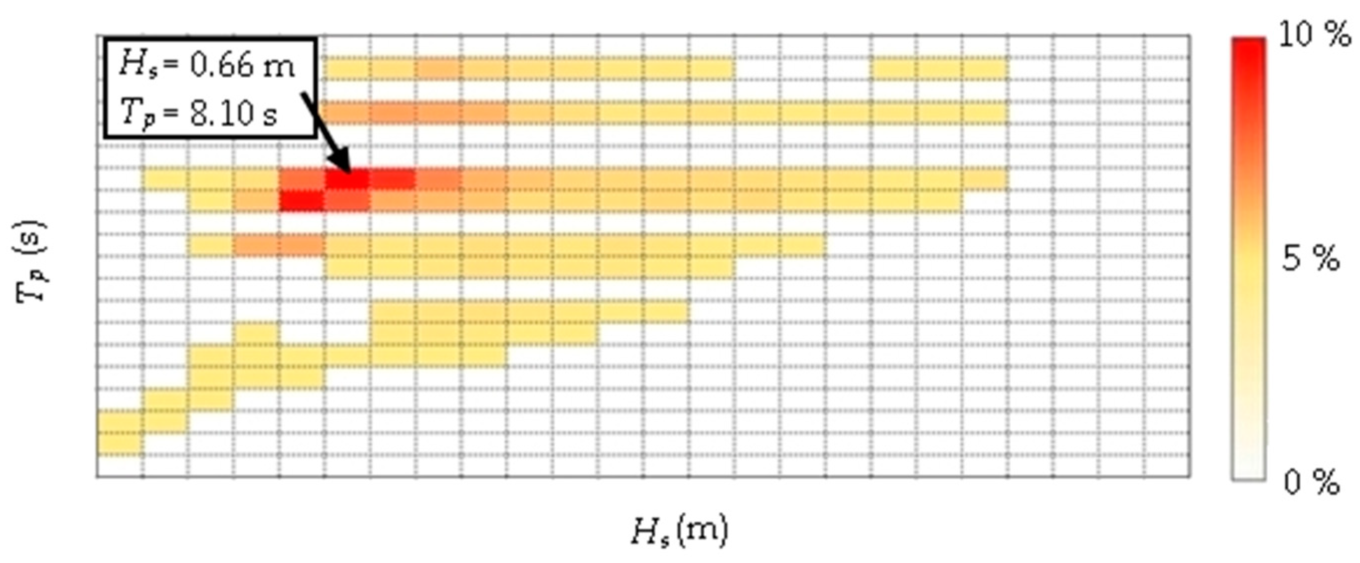
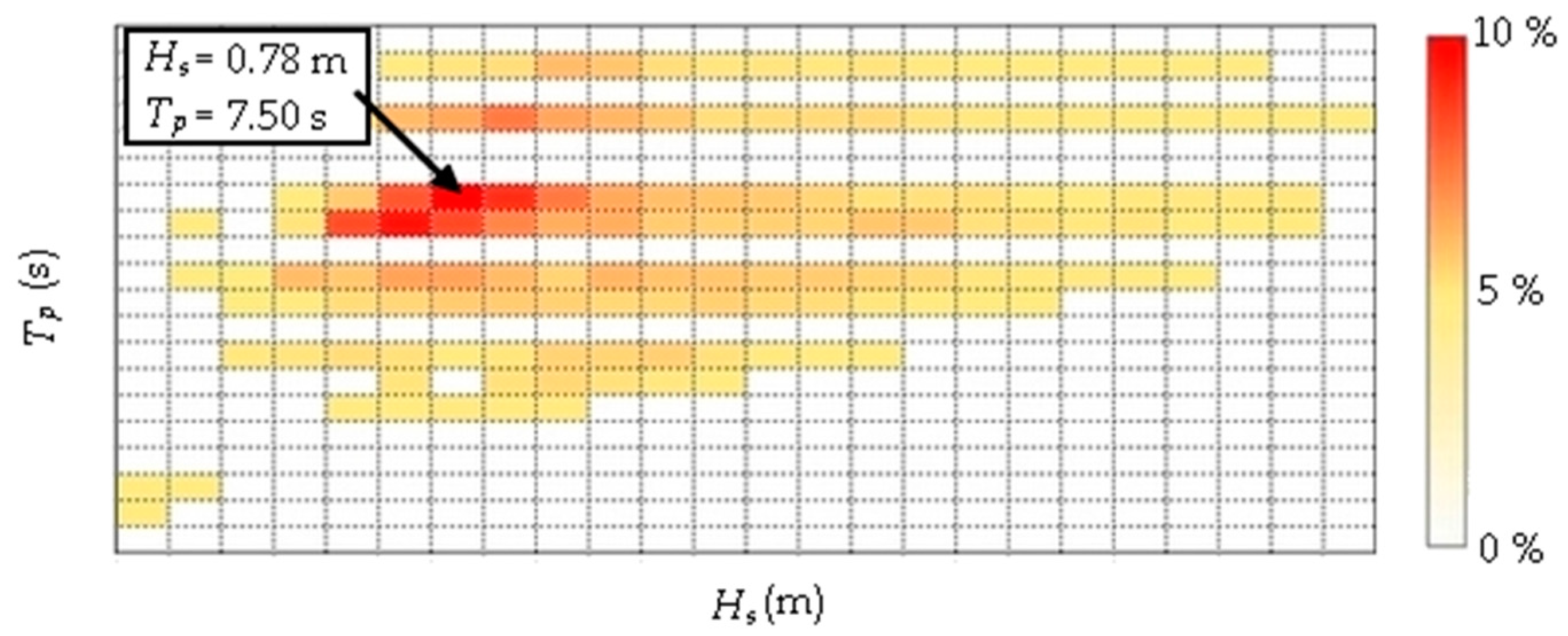
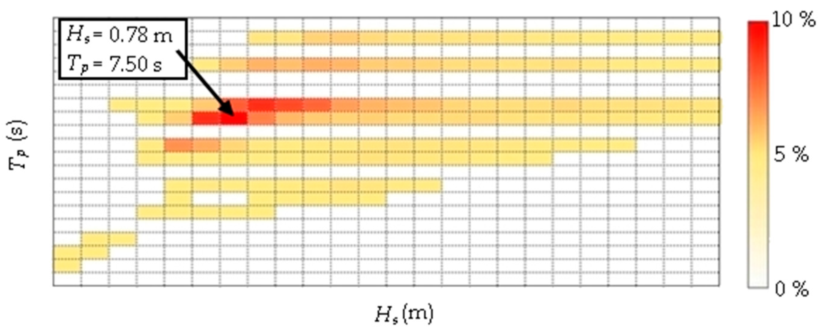
| Point | Height—H (m) | Period—T (s) | (m) |
|---|---|---|---|
| RG | 0.66 | 8.10 | 85.98 |
| SVP | 0.78 | 7.50 | 68.48 |
| TV | 0.78 | 7.50 | 68.48 |
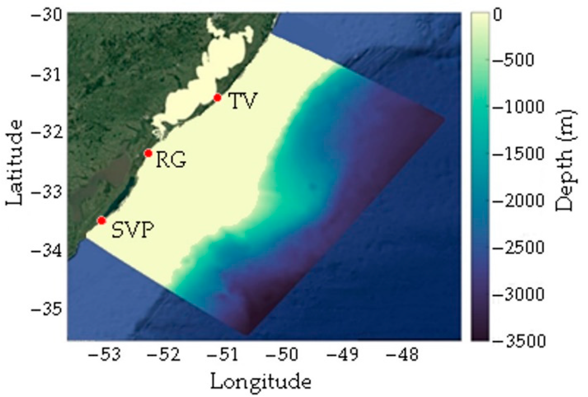
| Point | Date | Time (h) | Geographic Location | Depth—h (m) |
|---|---|---|---|---|
| RG | 8 September 2014 | 8.25 | −52° 17″ 47.25′ W, −032° 22″ 30.95′ S | 9.52 |
| SVP | 31 July 2014 | 18.5 | −53° 04″ 29.27′ W, −033° 32″ 42.47′ S | 11.09 |
| TV | 24 February 2014 | 12.75 | −51° 06″ 20.37′ W, −031° 27″ 7.97′ S | 13.97 |
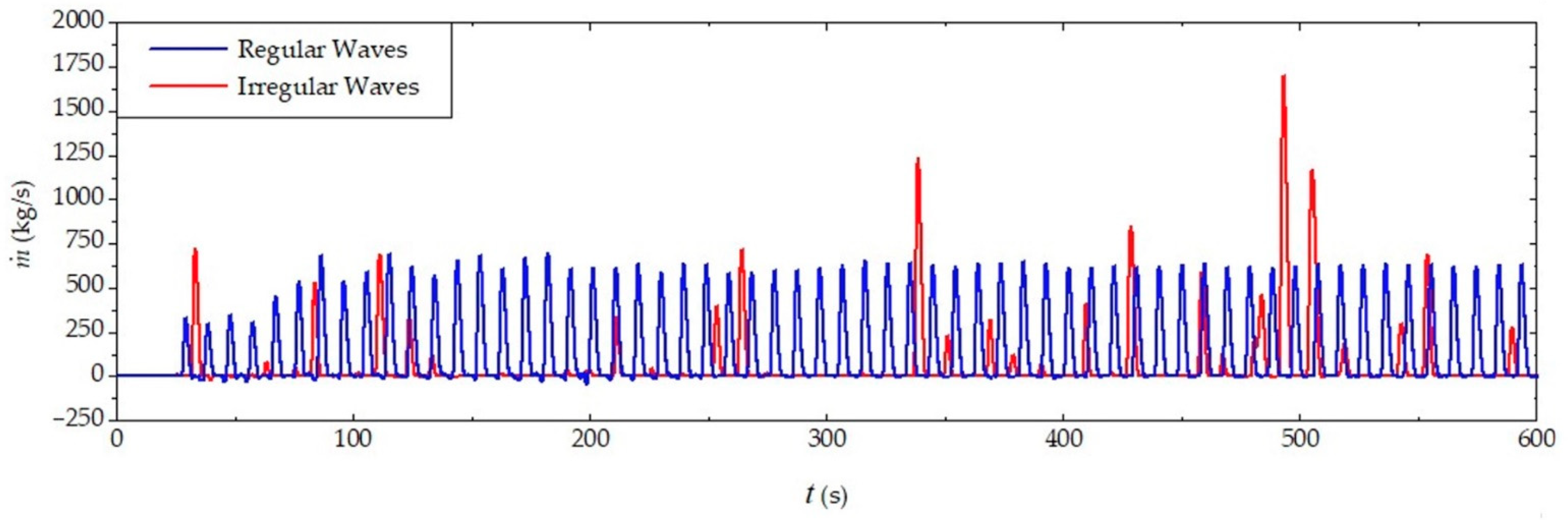
| Location | Wave | First-Degree Polynomial | Time Range | |
|---|---|---|---|---|
| RG | Regular | s | 0.9997 | |
| Irregular | s | 0.9491 | ||
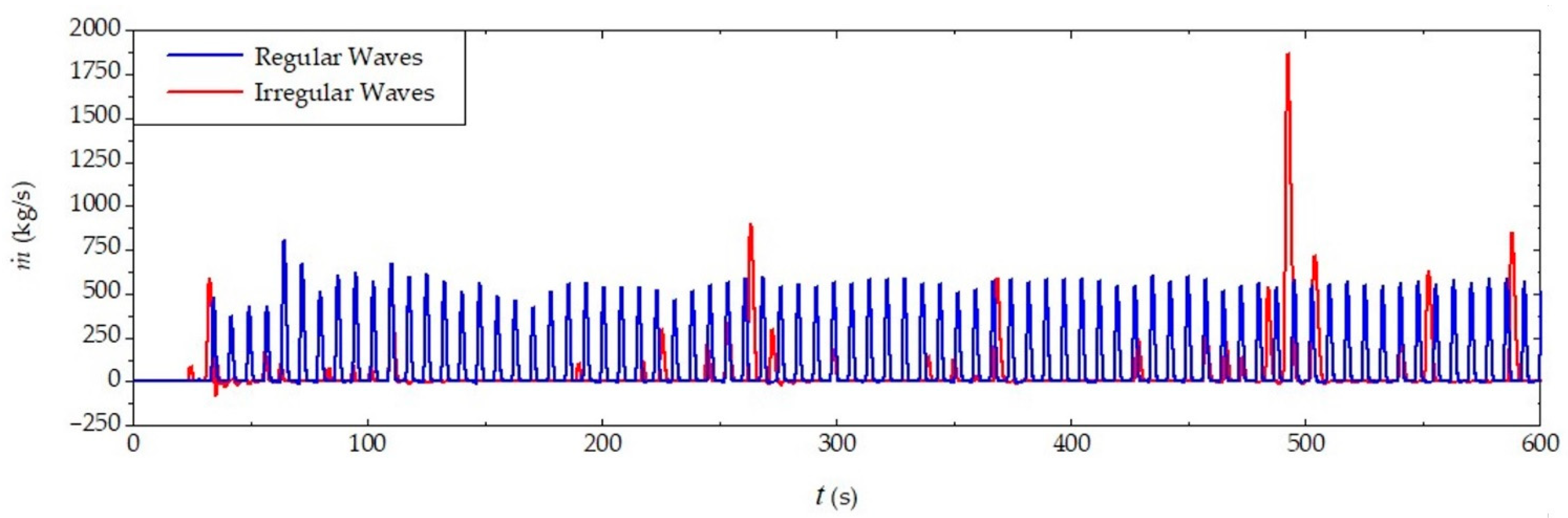
| SVP | Regular | 0.9998 | ||
| Irregular | s | 0.9456 | ||
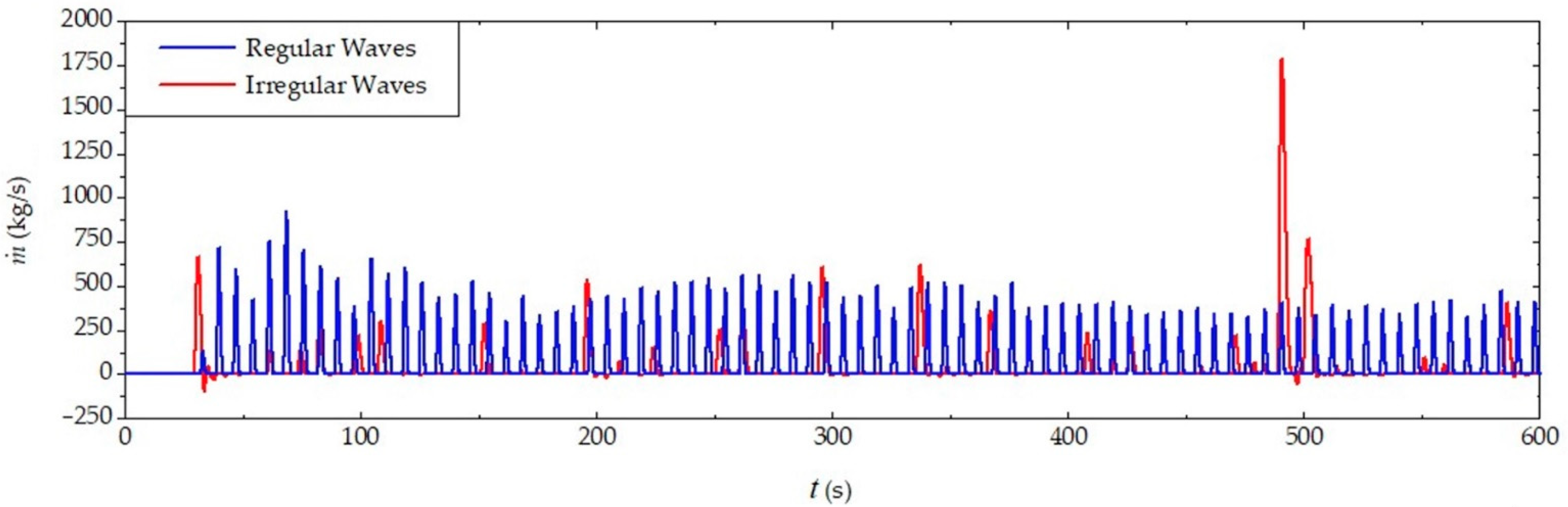
| TV | Regular | s | 0.9976 | |
| Irregular | s | 0.9684 |
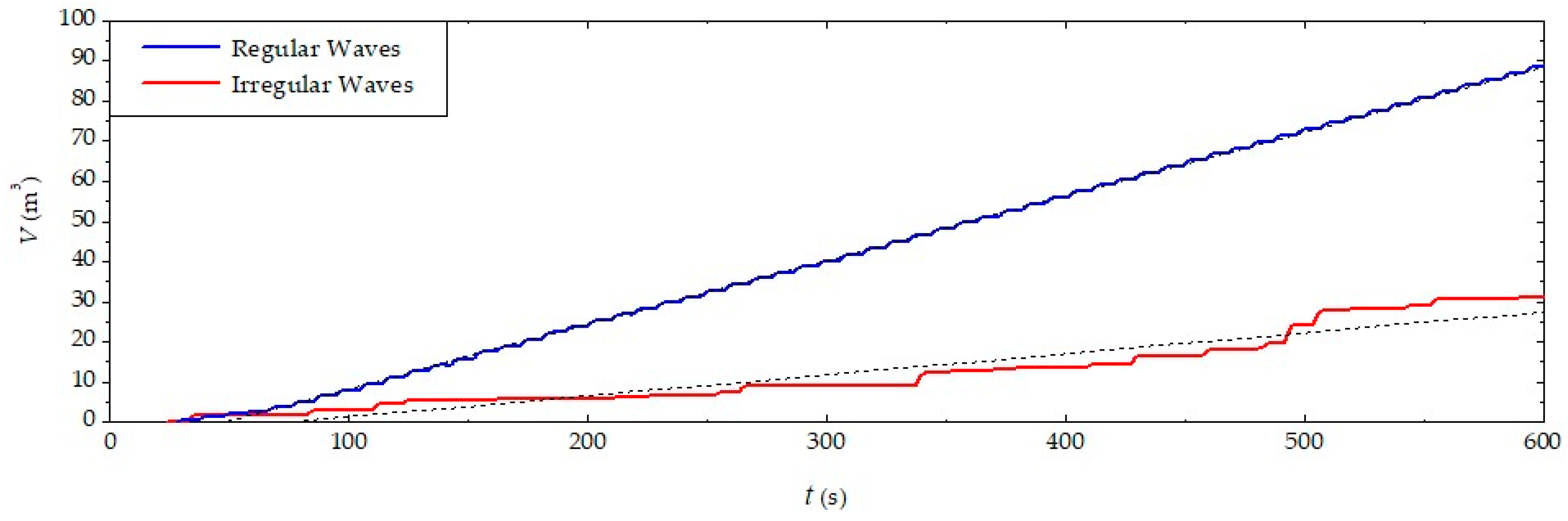
| Location | Wave | Water Volume (m3) |
|---|---|---|
| RG | Regular | 88.54 |
| Irregular | 31.26 | |
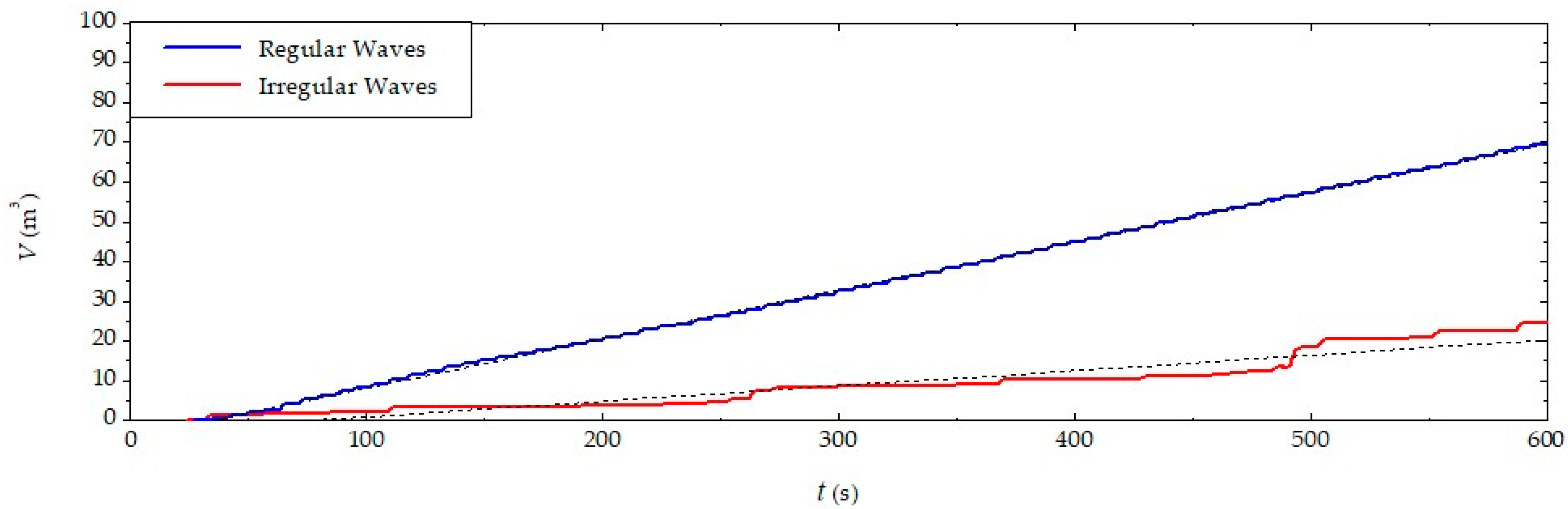
| SVP | Regular | 69.58 |
| Irregular | 24.51 | |
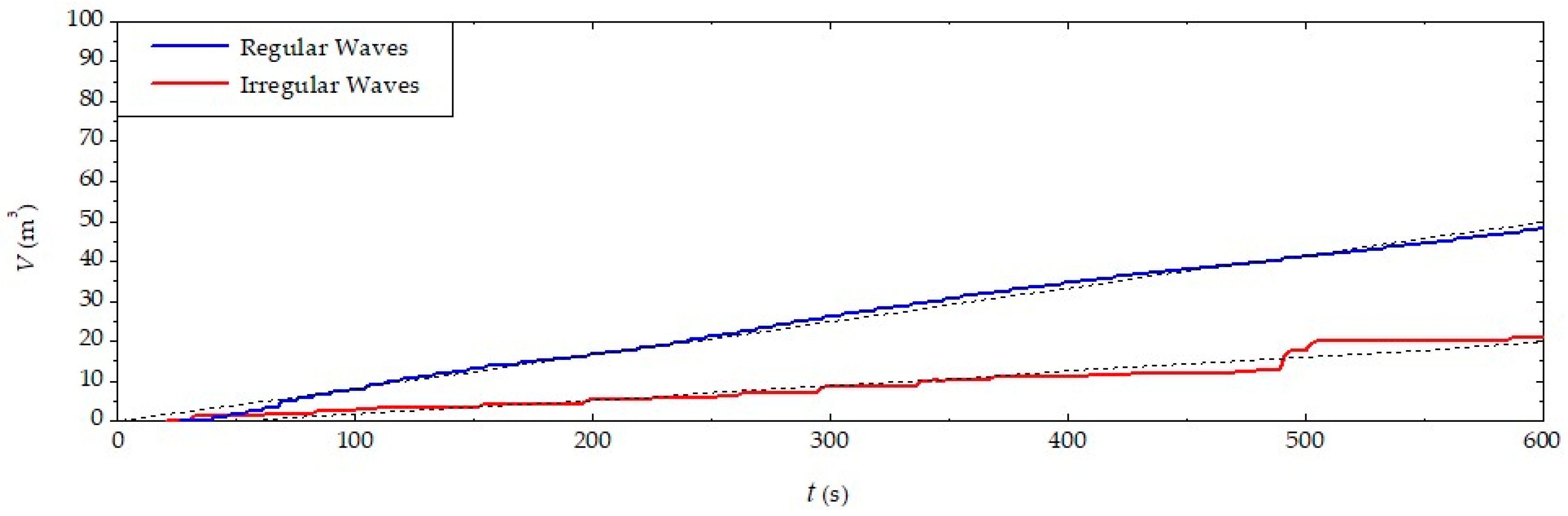
| TV | Regular | 48.19 |
| Irregular | 21.08 |
| Case | Wave | Water Volume (m³) | Difference (Times) |
|---|---|---|---|
| Present Study—RG | Regular | 8.02 | 2.69 |
| Irregular | 2.98 | ||
| Present Study—SVP | Regular | 8.34 | 4.01 |
| Irregular | 2.08 | ||
| Present Study—TV | Regular | 8.01 | 2.83 |
| Irregular | 2.83 | ||
| Martins et al. [50] | Regular | 15.32 | 3.78 |
| Pierson–Moskowitz | 4.05 |
Publisher’s Note: MDPI stays neutral with regard to jurisdictional claims in published maps and institutional affiliations. |
© 2022 by the authors. Licensee MDPI, Basel, Switzerland. This article is an open access article distributed under the terms and conditions of the Creative Commons Attribution (CC BY) license (https://creativecommons.org/licenses/by/4.0/).
Share and Cite
Hubner, R.G.; Fragassa, C.; Paiva, M.d.S.; Oleinik, P.H.; Gomes, M.d.N.; Rocha, L.A.O.; Santos, E.D.d.; Machado, B.N.; Isoldi, L.A. Numerical Analysis of an Overtopping Wave Energy Converter Subjected to the Incidence of Irregular and Regular Waves from Realistic Sea States. J. Mar. Sci. Eng. 2022, 10, 1084. https://doi.org/10.3390/jmse10081084
Hubner RG, Fragassa C, Paiva MdS, Oleinik PH, Gomes MdN, Rocha LAO, Santos EDd, Machado BN, Isoldi LA. Numerical Analysis of an Overtopping Wave Energy Converter Subjected to the Incidence of Irregular and Regular Waves from Realistic Sea States. Journal of Marine Science and Engineering. 2022; 10(8):1084. https://doi.org/10.3390/jmse10081084
Chicago/Turabian StyleHubner, Ricardo G., Cristiano Fragassa, Maycon da S. Paiva, Phelype H. Oleinik, Mateus das N. Gomes, Luiz A. O. Rocha, Elizaldo D. dos Santos, Bianca N. Machado, and Liércio A. Isoldi. 2022. "Numerical Analysis of an Overtopping Wave Energy Converter Subjected to the Incidence of Irregular and Regular Waves from Realistic Sea States" Journal of Marine Science and Engineering 10, no. 8: 1084. https://doi.org/10.3390/jmse10081084
APA StyleHubner, R. G., Fragassa, C., Paiva, M. d. S., Oleinik, P. H., Gomes, M. d. N., Rocha, L. A. O., Santos, E. D. d., Machado, B. N., & Isoldi, L. A. (2022). Numerical Analysis of an Overtopping Wave Energy Converter Subjected to the Incidence of Irregular and Regular Waves from Realistic Sea States. Journal of Marine Science and Engineering, 10(8), 1084. https://doi.org/10.3390/jmse10081084