Abstract
Many populated, tropical coastlines fronted by fringing coral reefs are exposed to wave-driven marine flooding that is exacerbated by sea-level rise. Most fringing coral reefs are not alongshore uniform, but bisected by shore-normal channels; however, little is known about the influence of such channels on alongshore variations on runup and flooding of the adjacent coastline. We conducted a parametric study using the numeric model XBeach that demonstrates that a shore-normal channel results in substantial alongshore variations in waves, wave-driven water levels, and the resulting runup. Depending on the geometry and forcing, runup is greater either on the coastline adjacent to the channel terminus or at locations near the alongshore extent of the channel. The impact of channels on runup increases for higher incident waves, lower incident wave steepness, wider channels, a narrower reef, and shorter channel spacing. Alongshore variation of infragravity waves is predominantly responsible for large-scale variations in runup outside the channel, whereas setup, sea-swell waves, and very-low frequency waves mainly increase runup inside the channel. These results provide insight into which coastal locations adjacent to shore-normal channels are most vulnerable to high runup events, using only widely available data such as reef geometry and offshore wave conditions.
1. Introduction
Fringing coral reefs serve as a natural coastal protection by dissipating a large portion of incident wave energy before reaching the shoreline. Depending on the reef geometry, reported values of wave attenuation vary from 60% to 99% [1,2] but diminishes for high water levels and large wave conditions [3,4], causing potentially high runup and large flooding during weather events.
The protection by coral reefs is important because the consequences of marine flooding of coastal land adjacent to coral reefs are significant. More than 50% of the total population of Pacific Islands lives within 1.5 km of the shoreline [5] and thus most of these population centers are vulnerable to coastal flooding due to their low elevation [6]. Even on high islands, the presence of steep terrain causes the majority of population, infrastructure (housing, businesses, ports, airports, power plants, sewage treatment plants, etc.), and economic activity to be concentrated on a narrow strip along the coastline susceptible to marine flooding. Locations where the reef is bisected by a shore-normal channel extending from the fore reef to the shoreline (Figure 1) are especially attractive for population centers, as channels provide a natural harbor, easy access to deeper water for vessels, and drinking water supply through streams. These locations may not be protected by the fringing reefs due to the channel incisions.
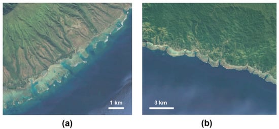
Figure 1.
Examples of shore-normal channels in fringing coral reef platforms. (a) Moloka’i, Hawai’i. (b) Viti Levu, Fiji.
Research is ongoing on this subject to understand which hydrodynamic processes lead to these high runup levels, and some valuable insights have been gained [7,8,9]: the recent increases in oceanic flooding along reef-lined coasts are primarily due to high offshore water levels coinciding with high energy wave events [3,9,10], circumstances which will become more frequent with sea-level rise [11,12]. Increasing water depth over the reef changes the hydrodynamics across the reef in such a way that larger waves reach the shoreline [13], causing high runup levels and flooding of the land behind the shoreline [3,4].
However, most previous research on runup has been based on one-dimensional (1-D) schematization of coral reefs [3,7,10], representing a uniform and straight coastline, whereas most reefs have significant alongshore bathymetric variability. Alongshore variations on coral reef morphology lead to mean currents and circulation that affect nutrient transport [14,15] and hence coral development. Furthermore, mean currents and processes such as wave diffraction and refraction change the directional wave spectrum and can affect alongshore sediment transport [16,17] and wave-driven runup. Previous studies that have investigated alongshore variations in reefs [18,19,20] usually addressed barrier reef-lagoon systems rather than the more common fringing reefs, and focused on setup differences and flushing times rather than the waves, water levels, and resulting runup at the shoreline. The one study that specifically investigated two-dimensional (2-D) wave processes on fringing reef platforms [21] used a sea-swell (“S”, periods < 25 s) wave model that did not include the effects of longer infragravity (“IG”, 25 s < periods < 250 s) and low-frequency (“VLF”, periods > 250 s) waves, which are important for wave-driven water levels and runup on such reef morphologies [3,4,8].
As of this time, no studies have been performed on the influence of shore-normal reef channels on flooding along fringing reef-lined coasts, specifically during extreme wave conditions when the risk for coastal flooding and the resulting impact to coastal communities is greatest. To address this knowledge gap, we used the physics-based numerical model, XBeach, which has previously been calibrated for fringing coral reefs, to conduct a parametric investigation of how variations in the reef and shore-normal channel morphology and oceanographic forcing influence waves, wave-driven water levels, and the resulting runup on fringing reef coasts.
2. Materials and Methods
2.1. Reef and Channel Morphologic Parameters
On the basis of Google Earth images, Rey [22] analyzed 70 fringing reef sections that had shore-normal channels and recorded their reef width, channel width, channel spacing, and channel angle. Reef width (Wr) was measured next to the channel, perpendicular to the coastline (Figure 2, Appendix A Table A1). Most reefs have a Wr of approximately 300 m, which was the value in the baseline scenario for the numerical modeling. However, the standard deviation in the dataset is large, and thus Wr, was varied from 100 to 1000 m between simulations. Channel width (Wc) was the average channel width of the channel, perpendicular to the channel axis. Most channels have a Wc of approximately 100 m, which was the value in the baseline scenario; Wc was varied from 50 to 300 m between simulations. The channel spacing (Sc) was measured on the two reef sections on both sides of the channel. Most observed Sc are on the order of 1000 m, which was used as the baseline value. Again, the standard deviation in the dataset is large; thus, Sc was varied from 300 to 2000 m between simulations. In most cases, the channel is perpendicular to the coastline, or less than 5 degrees. To keep the baseline scenario simple, the channel was perpendicular to the coastline. Rey [22] also summarized data from 15 previous studies of fringing reefs and recorded their fore reef (ifore) and beach slopes (ibeach). Based on the most common values, in the baseline scenario, both ifore and ibeach had values of 1 in 10. Inside the channel, ibeach extended below the waterline, and was thus also 1 in 10.

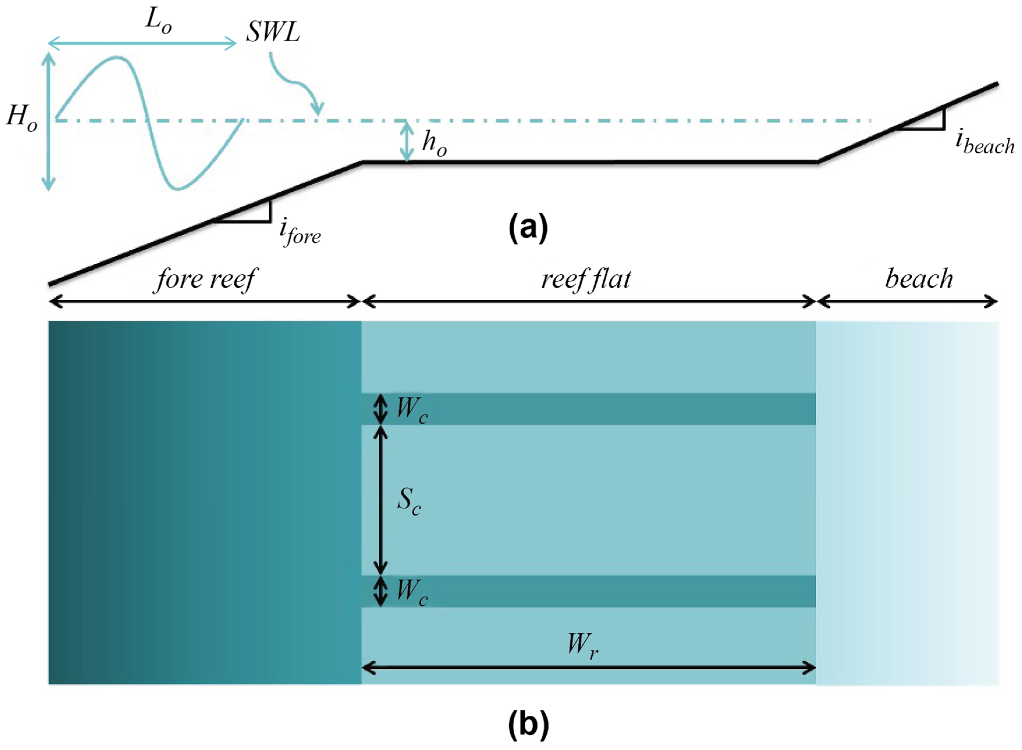
Figure 2.
Terminology of reef and channel geomorphology and oceanographic forcing. (a) Cross-sectional view. (b) Map view, with darker colors denoting greater water depth. Geomorphic parameters include reef width, Wr. channel width, Wc. channel spacing, Sc, fore reef slope (ifore), and beach slope (ibeach). Oceanographic parameters include offshore significant wave height, Ho, offshore peak wave period, Tp, and reef flat water depth, ho, relative to the still water level, SWL.
2.2. Oceanographic Forcing Parameters
Most atoll and fringing reefs are exposed to both episodic tropical cyclones and large swell events, but the latter are responsible for the majority of documented past high runup events and flooding of reef-lined coasts [4,9]. The primary interest of this study was not the weather extremes that only occur once in a lifetime, but rather episodic events that occur approximately yearly and are a regular nuisance to inhabitants of coastal regions protected by atoll and fringing reefs. Therefore, yearly maxima of 30 years of hindcasted wave conditions developed by Shope et al. [23] were used as the forcing in this study. For the baseline scenario, a significant offshore wave height (Ho) of 5 m was applied with a wave steepness (ratio of Ho to offshore wavelength, Lo, thus Ho/Lo) of 0.02, corresponding to a peak wave period (Tp) of 12.8 s based on the average range (Figure 2, Appendix A Table A1). In the simulations, Ho was varied from 3 to 7 m, corresponding to the yearly maximum wave height ±2 standard deviations, covering 95% of naturally occurring values; Ho/Lo was varied from 0.01 to 0.03, corresponding to the maximum and minimum observed values. For simplicity, in the baseline scenario, the waves approached the coast perpendicularly with no directional spreading. In terms of water levels, most atoll and fringing reef flats have still water depths (ho) of 0.3 to 2.0 m, with an average of 1.0 m [3]. The greatest runup elevations (total water levels) are greatest for deeper ho, but runup is driven largely by setup differences, which are largest when ho is small [3]. To gain insight into both setup and runup, the baseline scenario had an ho of 1 m, which was not varied between simulations.
A total of 135 simulations were performed: A combination of 9 different oceanographic forcing scenarios (Ho = 3, 5, 7 m and Ho/Lo = 0.01, 0.02, 0.03), each applied to 15 reef geomorphologies: 4 reference scenarios (simulations of reefs with Wr = 100, 300, 500, 1000 m but without a channel), the baseline geometry, 4 variations in Wc (50, 70, 200, 300 m), 3 variations in Wr (100, 500, 1000 m), and 3 variations in Sc (300, 600, 2000 m).
2.3. Numerical Modeling
2.3.1. Model Overview
To understand the influence of alongshore variations in reef geomorphology on waves, water levels, and runup, the physics-based, 2-dimensional (2D) XBeach Non-Hydrostatic (XB-NH) (Deltares, The Netherlands) model was used. XBeach is a process-based, depth-averaged numerical model, which includes a number of hydrodynamic processes such as short and long wave transformation, wave-induced setup, unsteady currents, and overwash [24,25,26]. It was originally developed to simulate hydrodynamic and morphodynamic processes on sandy coasts during storm events. Subsequently, has been applied to a wider range of modeling situations, such as gravel [27] and vegetated coasts [28]. The XBeach model has successfully been applied to coral reef environments in numerous studies [3,7,29,30,31,32].
XBeach has two modes, the phase-averaged XBeach Surf Beat (XB-SB) and XB-NH, the latter being phase resolving [26,33]. XB-NH resolves the wave field on the timescale of individual waves, and the model is capable of accurately resolving the non-linear evolution of the wave field, wave–current interaction, and wave breaking in the surf zone [34]. Because the non-hydrostatic mode solves for both long and short waves on the individual wave scale, it is more accurate regarding individual wave breaking and short wave runup than the hydrostatic mode. Here, we used the computationally more expensive XB-NH, as the focus of this study was runup, and it was shown by [3,32,35] that to accurately reproduce wave runup on coral reef-lined coasts, short wave processes cannot be ignored.
2.3.2. Model Settings
In the baseline scenario, the reef has a Wr of 300 m, with a Wc of 100 m, and a Sc of 1000 m. Cyclic boundary conditions were applied on the lateral boundaries, which translate to a 100 m wide channel in the middle of the grid, with an adjacent reef flat of 500 m alongshore on both sides. For simplicity reasons, the channel has a triangular cross section extending to a depth of the base of the reef at 30 m and sloping offshore at the same gradient as ibeach. At the offshore boundary, the grid was extended to a depth of 30 m followed by 20 horizontal grid cells for a 30 m flat section before the wavemaker. At the shoreward boundary, the model was extended to +12 m with an ifore of 1:10 to account for very high runup levels. A rectangular grid was applied. The alongshore grid resolution varied between 1 m in the channel to 4 m near the boundaries. The cross-shore grid size had a maximum resolution of 0.5 m at the shoreline, corresponding with a 0.05 m vertical resolution for an ibeach of 1:10, and a minimum resolution of 1.5 m farther offshore. With an ibeach of 1:10, the vertical resolution was 5 cm at the shoreline. A maximum smoothness, defined as the ratio between cell sizes of two adjacent cells, of 1.05 was applied.
The sediment transport and morphological change were disabled. Bottom friction was accounted for by use of the friction coefficient, cf. For the rough fore reef, a cf of 0.04 was applied, and for the smoother reef flat and beach, a cf of 0.002 was used, based on the cf values used in 2-D XBeach reef studies by [12,30].
All of the input wave time series were derived from the same Jonswap spectrum, and were thus identical for all simulations. The offshore water level was kept constant and uniform alongshore. Those time series were applied consecutively at the offshore boundary. Because the hydrodynamic patterns reached a dynamic equilibrium in 1000 s, a conservative spin-up time of 1500 s was applied. Ru2%, defined as the average runup of the highest 2% of waves, requires a large number of waves reaching the coastline during the simulation for accurate computation. It is common practice to calculate the Ru2% over 1000 waves [3] so the Ru2% is the average of the 20 highest waves. After 6 h of runtime, the difference relative to the long-term mean Ru2% value was less than 20%, meaning that most of the variations had damped out, decreasing the influence of occasional high waves on the Ru2%. Therefore, a balance between ideal results and practical runtime was found at a simulated time containing 1500 waves, corresponding with a simulation time of slightly less than 6 h for a Tp of 12.8 s.
Hydrodynamic results were recorded at the offshore boundary, the last point of a water depth of 30 m, midway on the fore reef at 15 m depth, 20 m in front of the reef crest, at the reef crest, 20 m behind the reef crest, midway on the reef flat, and at the beach toe. To generate runup output, numerical runup gauges recorded the instantaneous runup level at 0.5 s intervals. Runup gauges were placed along the entire shoreline, at 2 m along-shore intervals within 120 m of the channel, and at 4 m intervals along the remaining shoreline.
2.3.3. Model Validation
Although it would be ideal to calibrate and validate a numerical model with field or laboratory data, to the best of our knowledge, no suitable data are available for this study: no runup or hydrodynamic data are available for coral reefs with channels. However, two factors mitigate the need to calibrate the numerical model on measured data. First, the goal of this conceptual study was not to replicate one case study perfectly, but instead to gain general insights into how the alongshore runup pattern varies in the presence of a shore-normal channel in the reef depending on the local reef geomorphology and oceanographic forcing, and to relate these patterns to dimensionless parameters. Second, as stated before, XB-NH has been applied numerous times for 1-D and 2-D modeling studies [3,7,26,32]. In those studies, the model was calibrated and validated against field and laboratory data, and performed satisfactorily; thus, XB-NH has proven its applicability to coral reef studies and can be used to explore the effects of shore-normal channels in reefs in a conceptual study.
3. Results
For all 135 XB-NH model simulations performed, the results were analyzed for reef hydrodynamics and the resulting runup. First, a description of the general trends in the influence of the channel on waves and setup is presented using the reference simulation of a 300 m wide reef flat with a 100 m wide channel being impacted by 7 m at 15 s waves. Next, a description of the general alongshore trends in runup is presented. To better understand what drives runup differences, the contribution of different frequency components to runup are then discussed. Finally, the influence of varying oceanographic forcing and reef and channel geomorphology on runup is assessed by comparison to simulations without a reef channel.
3.1. Influence Channels on Waves and Water Levels
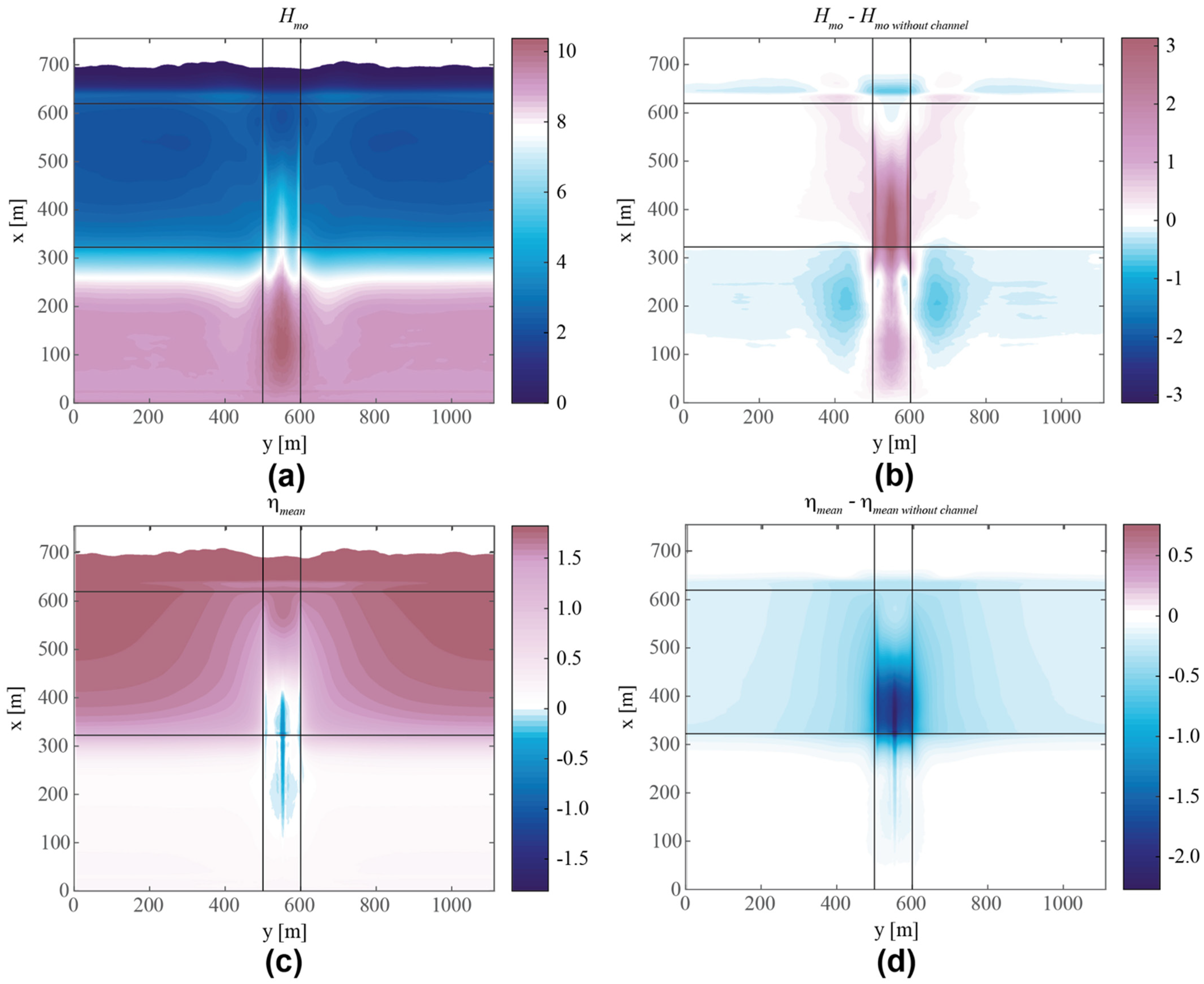
Significant total (SS + IG) wave height, Hm0, is calculated from the variance of the water level. The influence of the channel is assessed by subtracting Hm0 from Hm0 in the reference run without a channel. Hm0 is largest offshore the reef from the channel, in line with the channel (Figure 3a,b). Waves break in front of the reef crest and continue to decrease towards the shoreline. There is a high alongshore gradient of Hm0 in the channel. Comparing simulations with and without a channel, the differences are from −3 to +3 m (±42%), indicating the channel has a large influence on wave transformation. There is a relative increase in Hm0 inside the channel and a decrease in Hm0 offshore next to the channel. On the reef flat, the cross-shore difference in Hm0 is small, but at the shoreline there is an alongshore pattern of decreased Hm0 mid-reef and in the channel, and an increase in Hm0 next to the channel.

Figure 3.
Map views of wave height and setup across the reef for large (Ho = 7 m) and long-period (Tp = 15 s) offshore waves. (a) Mean wave height, Hm0. (b) Mean wave height, Hm0, relative to the reference run with the same forcing but without a channel. (c) Mean setup, ηmean. (d) ηmean, relative to the to the reference run with the same forcing but without a channel. The red zones indicate higher values in the case with a channel as compared to the reference case without a channel, and the blue zones indicate smaller values in the case with a channel. In these plots, offshore is on the bottom at x = 0, the reef crest at x = 320 m, and the still-water shoreline at x = 620 m; the channel extends from y = 500–600 m.
The mean setup (ηmean) is calculated as the mean water level over the entire simulation, and the influence of the channel is assessed by locally subtracting ηmean from ηmean in the reference run without a channel. Wave forcing causes ηmean on the reef flat up to 1.5 m (Figure 3c). In the channel, in the vicinity of the reef crest, ηmean is lower than the SWL, whereas near the shoreline, the setup is positive, decreasing alongshore from mid-reef towards the channel. The channel decreases ηmean up to 2 m (Figure 3d). The difference is greatest in the channel near the reef crest and decreases with increasing distance from the channel. ηmean increases shoreward from the reef crest towards the beach toe, and alongshore from the channel towards the mid-reef. There is a steep gradient in ηmean on the channel edge.
Thus, Hm0 was found to decrease towards the shoreline, whereas ηmean increases towards the shoreline. Variations of Hm0 and ηmean are most notable within 100 m from the channel, whereas the runup pattern displays strong variation for twice that distance. Both Hm0 and ηmean have sharp gradients around the channel edge.
3.2. Alongshore Patterns in Runup
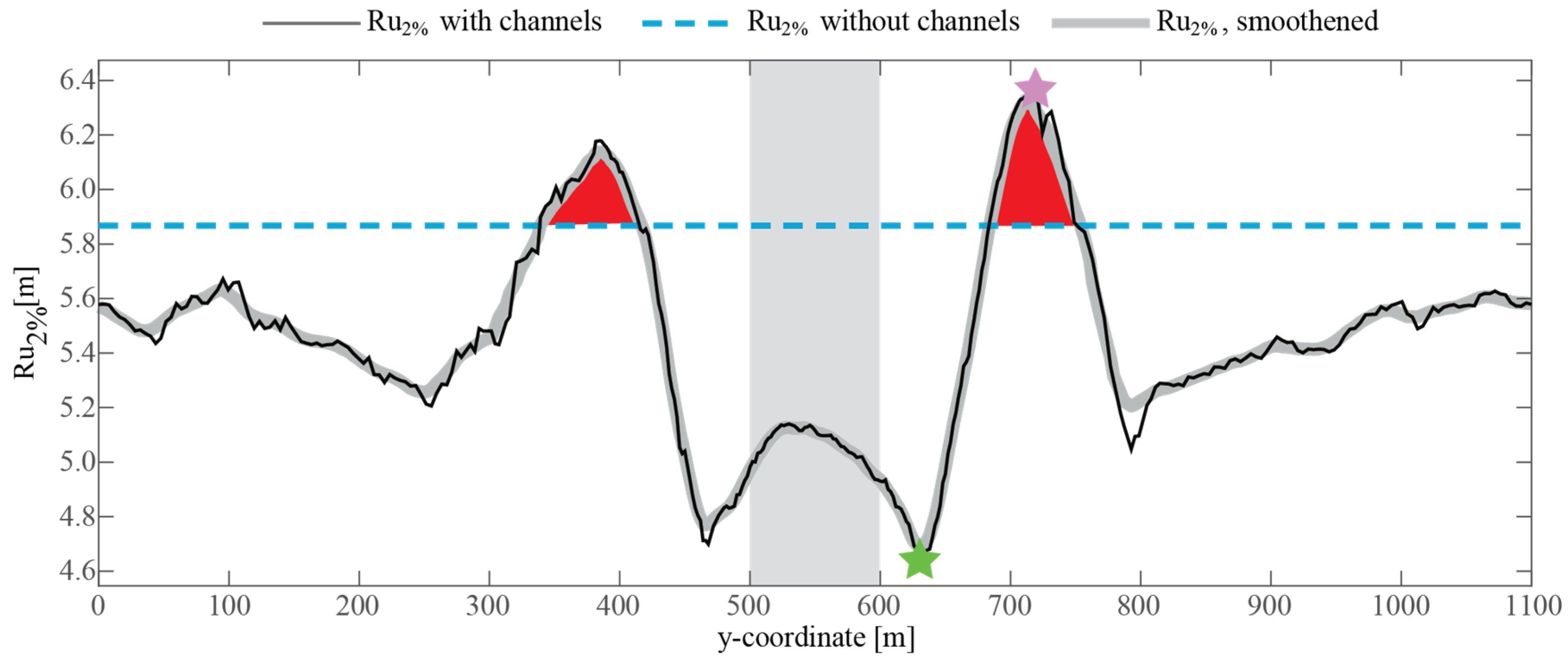
To assess the influence of the shore-normal reef channel on Ru2%, the scenarios with a channel were compared to the reference runs without a reef channel (Figure 4). There is alongshore variability in Ru2%, with a range of approximately 20% of Ho. The lack of perfect symmetry across the channel is due to the irregular SS and IG waves interacting with the reef morphology. The highest Ru2% (peak in Ru2%) is 5% higher in the simulation with a channel than without, and the lowest Ru2% (trough in Ru2%) is 15% lower with the channel without. The maxima (peaks) in Ru2% are approximately 120 m away from the channel edges, the minima (troughs) in Ru2% are found within approximately 40 m of the channel edges, and there is a local Ru2% maximum in the middle of the channel. The Ru2% in the middle of the reef (far from the channel) is 5% lower in the simulation with a channel than in the reference run.
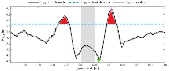
Figure 4.
Alongshore patterns in runup, Ru2%, for the reference case of a reef flat (Wr = 300 m) without a channel (dashed line) and with a channel (solid line) under identical large (Ho = 7 m) and long-period (Tp = 15 s) offshore waves. High runup zones where Ru2% exceeds the reference Ru2% are indicated by the red regions. The peak in Ru2% is indicated by a purple star; the lowest Ru2% is indicated by the green star. The gray region denotes the location of the channel (Wc = 100 m).
3.3. Frequency Components of Runup
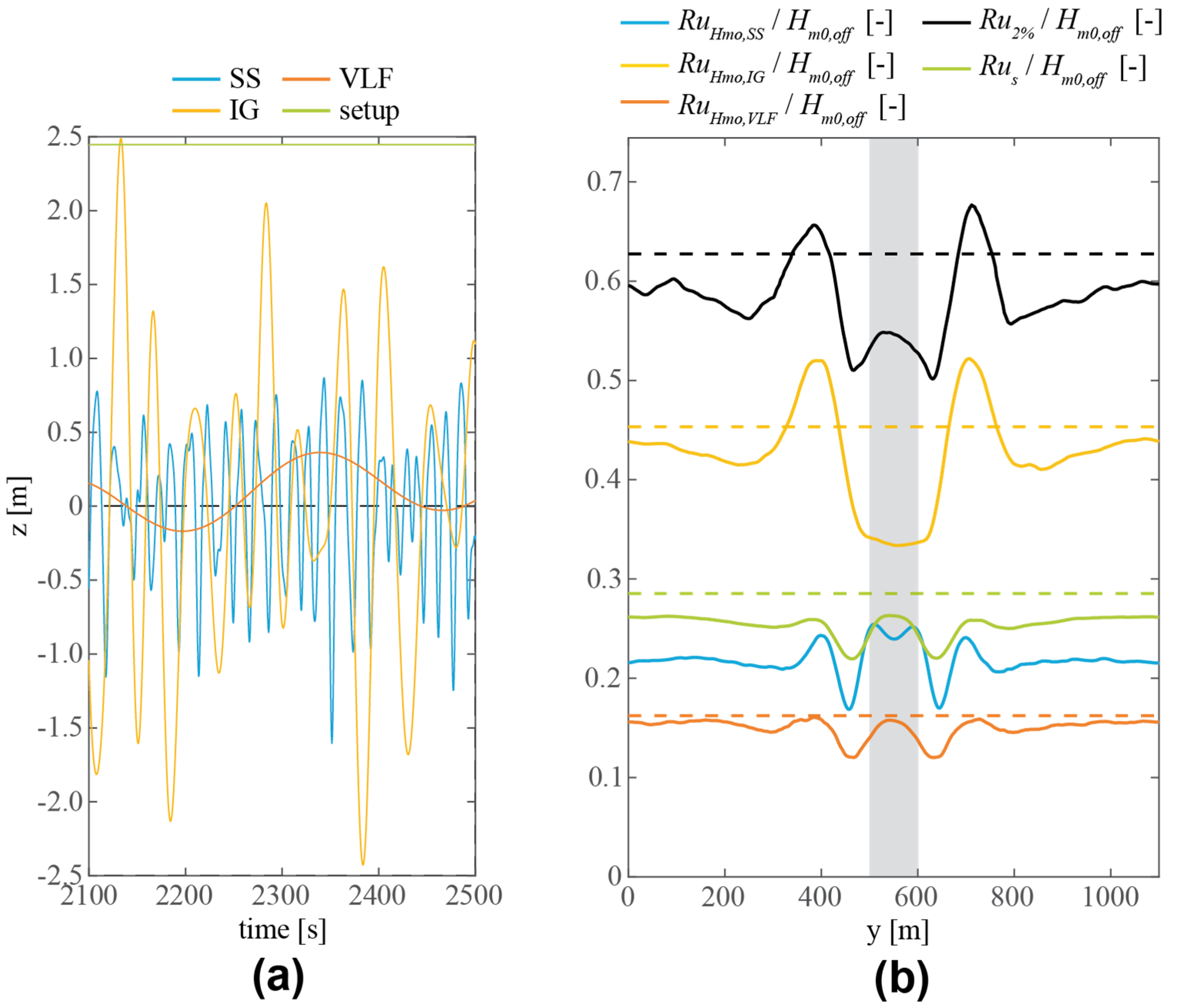
To better understand which wave processes are responsible for the differences in Ru2% alongshore, the influence of different frequency components on Ru2% was assessed. For each runup gauge, the vertical runup signal was split into setup (mean over entire run, Rus), SS (RuHmo,SS), IG (RuHmo,IG), and VLF (RuHmo,VLF) water level time series. From these time series, the runup height of each frequency component was calculated using the variance in the water level time series, which was normalized against Ho (Figure 5).
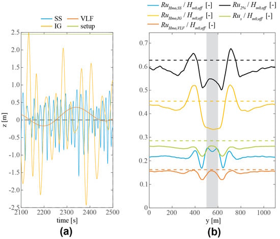
Figure 5.
Frequency components of waves and runup on the reef flat. (a) Time series of the SS (blue), IG (orange), VLF (red), and setup (green) components of water level, taken in the middle of reef by the shoreline. (b) Alongshore varying runup (Ru2%, black) split into setup (Rus, green), SS (RuHmo,SS, blue), IG (RuHmo,IG, orange), and VLF (RuHmo,VLF, red) wave components, presented as the fraction of the incoming waves by normalizing with wave height at the offshore boundary (Ho). The dashed lines in corresponding colors show the frequency components in the reference run without a channel. The gray region denotes the location of the channel.
RuHmo,IG is dominant, with RuHmo,IG up to 50% of the offshore Ho, which is approximately double the contribution of the other components. The RuHmo,IG peaks align with the Ru2% peaks, but the local Ru2% increase in the channel is not present in the RuHmo,IG. The vertical range is similar to the Ru2% range. In this simulation, Rus is the second largest contributor to Ru2%. The channel decreases Rus over the entire alongshore domain, as it is lower than in the reference run. The Rus peaks next to the channel align with Ru2% peaks, and also have a peak inside the channel that is present in the Ru2% pattern, but not in the RuHmo,IG. RuHmo,VLF is approximately half the Rus, with a similar alongshore pattern. RuHmo,SS only varies from the reference scenario in the vicinity of the channel, with peaks just inside the channel.
3.4. Influence of Geomorphology and Oceanographic Forcing on Runup
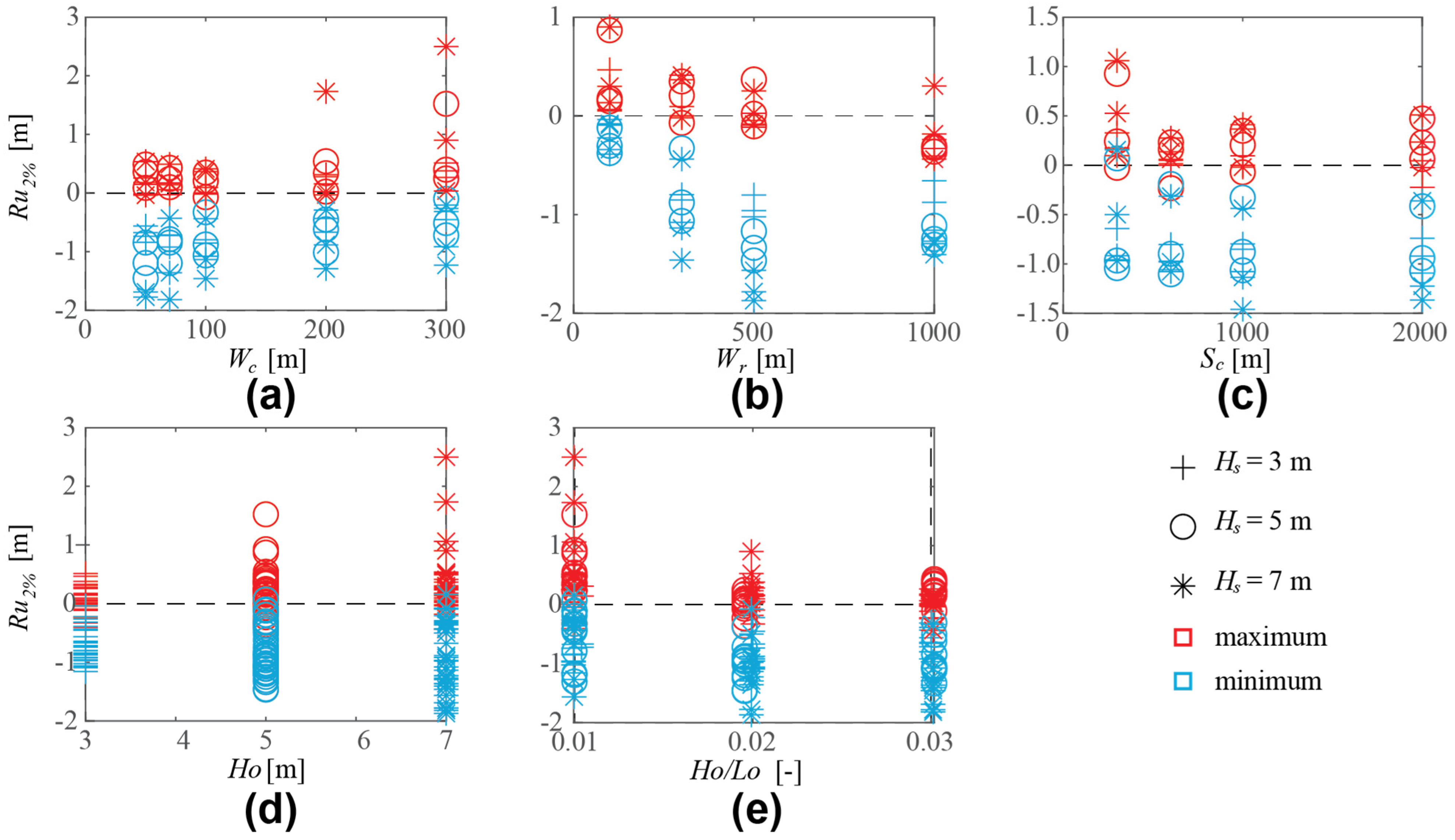
To assess the influence of the varying oceanographic forcing and reef and channel geomorphology on Ru2%, the maximum Ru2% of every simulation was compared to the three geomorphic (Wc, Wr, and Sc) and two forcing (Ho and Ho/Lo) parameters (Figure 6). The range of Ru2%, defined as the difference between the highest Ru2% peak and the minimum Ru2% peak, varies for different forcings on the same geometry; its range is approximately 20% of Ho. Ru2% maxima are higher for scenarios with higher Ho and low Ho/Lo, short Sc, narrower Wr, and wider Wc. Both Ho and Ho/Lo have a large influence on Ru2%. Of the geomorphic parameters, Wc has the strongest influence on Ru2%. Whereas Ru2% trends relatively linearly with the forcing (Ho and Ho/Lo) parameters, there are relatively non-linear response in Ru2% with changes in the geomorphic (Wc, Wr, and Sc) parameters, many of which have local minima.
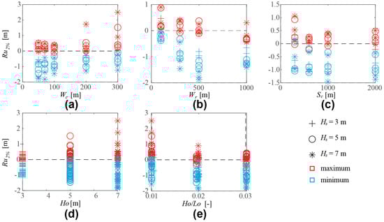
Figure 6.
Runup, Ru2%, for different reef and channel geomorphic parameters or oceanographic forcing parameters. (a) Channel width, Wc. (b) Reef width, Wr. (c) Channel spacing, Sc. (d) Significant wave height, Ho. (e) Wave steepness, Ho/Lo. The marker shapes indicate the Ho and colors the minimum or maximum values for a simulation.
4. Discussion
A shore-normal channel in a fringing reef strongly influences the overall Hm0 and ηmean patterns on the reef flat and in the channel. Alongshore gradients of Hm0 and ηmean are large in the vicinity of the channel. ηmean increases towards the shoreline and towards mid reef. Differences in Hm0 are most notable on the fore reef, in the channel, and at the shoreline. Hm0 and ηmean just offshore the beach toe have increasing correspondence with the Ru2% pattern, but still there are significant differences. There is a decrease in Ru2% in the vicinity of the channel, with a small increase inside the channel, a peak next to the channel, and a gradual approach of the reference Ru2% towards mid-reef. Sometimes, but not always, a local Ru2% peak occurs inside the channel.
Variations in both reef geomorphology and oceanographic forcing change one or more of the following characteristics. For small Ho and Ho/Lo, the Ru2% pattern does not show a clear peak, just a decrease in Ru2% towards the channel. High Ho/Lo and wide Wc both result in a dual Ru2% peak system with a second Ru2% peak inside the channel. Narrow Wr make the Ru2% pattern more alternating and irregular, whereas wide Wr decrease Ru2% compared to the reference Ru2% without a channel. Short Sc move the Ru2% peak towards mid-reef, whereas for long Sc, the longshore Ru2% variation stays restricted to the vicinity of the channel. The largest Ru2% peaks occur in the channel, for wide Wc and high Ho and Ho/Lo. Ru2% peaks are largest when Wc takes up a large fraction of the total shoreline and when the incident Tp is closer to the resonant period of the reef.
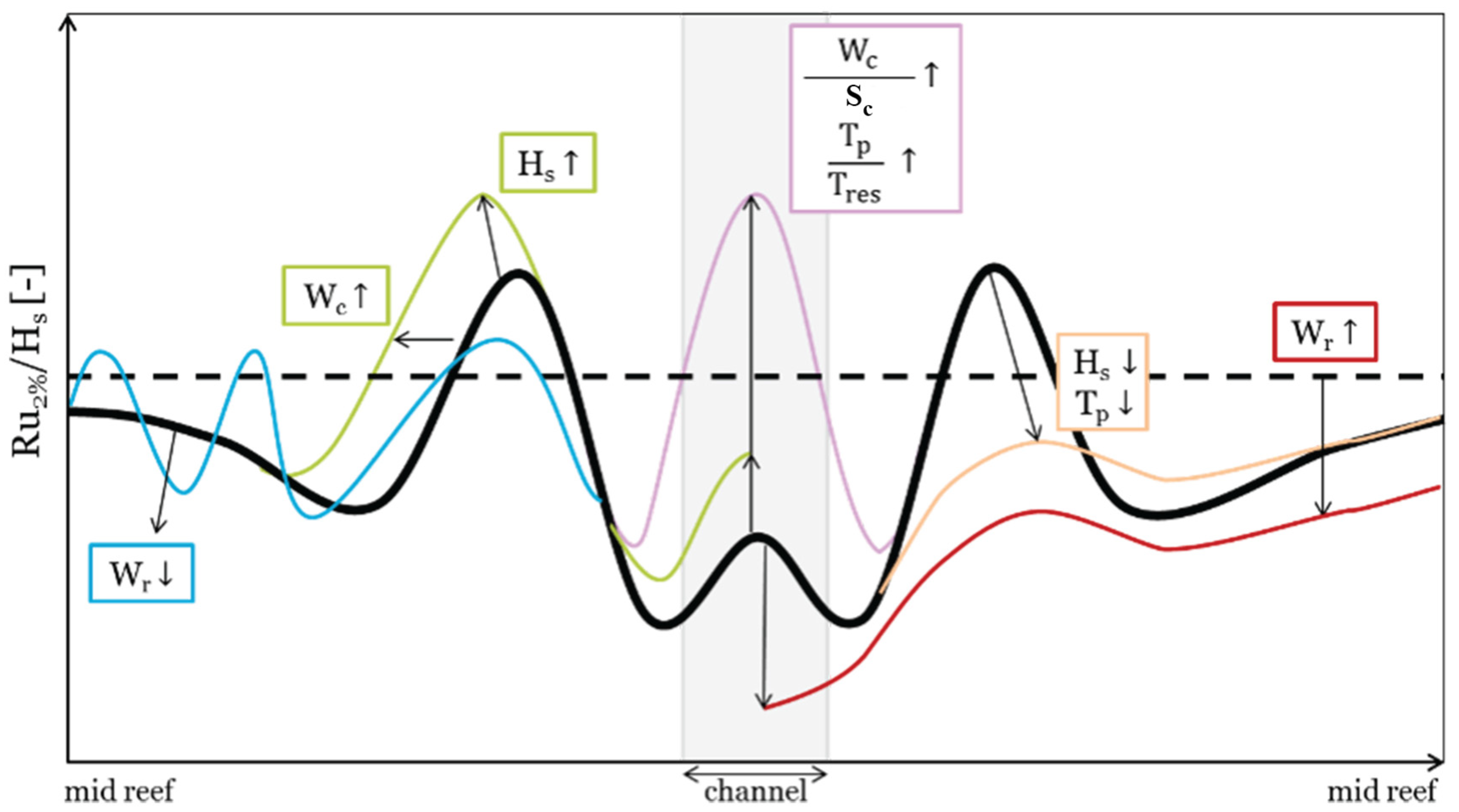
A schematic that illustrates the general Ru2% pattern, and the impact of each geomorphic or oceanographic parameter on this pattern, is presented in (Figure 7). This schematic illustrates the following conclusions regarding the alongshore variations in the Ru2% patterns:
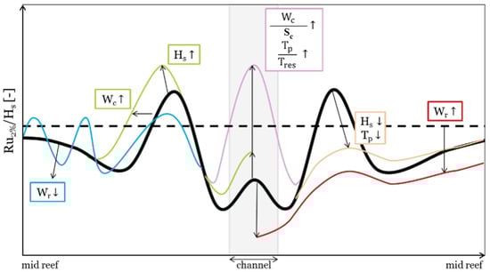
Figure 7.
Overview of runup pattern for variations in reef and channel geomorphology and oceanographic forcing. The solid black line shows the general alongshore runup pattern for a reef with a channel, and the dashed line represents the reference line for a case without a channel. The colored lines illustrate the influence of variations in forcing and geomorphology on changing patterns in runup relative to the base case (solid black line). Arrows denote the trends in change relative to the base scenario for the given parameter or ratio between the parameters. Portions of solid lines above the dashed line indicate alongshore areas, relative to the channel, where there is greater runup than in the case without a channel, and those below the dashed line indicate those alongshore areas with less runup.
- For small Ho and Ho/Lo, the Ru2% pattern does not show a clear peak, just a decrease in Ru2% towards the channel.
- Low Ho/Lo and wide Wc both result in a dual Ru2% peak system, with a second Ru2% peak inside the channel.
- Narrow Wr make the Ru2% pattern more alternating and irregular, whereas wide Wr decrease Ru2% compared to the reference Ru2% without a channel.
- Short Sc result in a Ru2% peak farther mid-reef, whereas for long Sc, the alongshore Ru2% variation is restricted to the vicinity of the channel.
- The largest Ru2% peaks occur in the channel, for wide Wc and high and high Tp waves. Ru2% peaks are greatest as the channel takes up a large fraction of the total shoreline when the Tp is closer to the resonant period of the reef.
In terms of the relative contribution of frequency components to Ru2% for varying geomorphologies and oceanographic forcing, IG waves are the dominant contributor. The shape is similar to the Ru2% pattern, except for the local peak inside the channel, and the contribution is larger than that of the SS, VLF, and setup components. This is in line with findings from 1-D Ru2% studies on reefs [3,4,7]. For waves with low Ho and high Ho/Lo, SS has the second-largest contribution to Ru2%, whereas, for waves with high Ho and low Ho/Lo, setup becomes increasingly important. This is in line with expectations, as setup is smaller for increasing relative reef submergence and Ho/Lo [8,18,36]. For simulations where the Ru2% is largely below the reference Ru2%, setup and VLF are also lower than their reference line, whereas alongshore mean SS and IG are near their reference level. This indicates VLF and setup are responsible for the global decrease in Ru2% alongshore. Variations in VLF and setup are mostly gradual and extend toward the mid-reef, whereas SS gradients are largest in the vicinity of the channel and do not vary much towards mid-reef; IG are between SS and VLF. This may indicate that the wavelength of a frequency component is linked to the region of influence from the channel of the given component. Further numerical and field studies may confirm this.
5. Conclusions
The results of this numerical model study illustrate the importance of 2-D effects for Ru2%. Most previous modeling studies of coral reefs have been based on 1-D schematizations, and it is expected that future studies will also be, due to the huge difference between computational demand, and hence runtime, of 1-D versus 2-D models. Whether it is justified to use a 1-D transect rather than a 2-D model depends on the distance from the channel.
The current results show that, even far from the channel, even at mid-reef, the channel still has influence on Ru2% levels, due to the decrease in setup. In the present study, the channel increases the Ru2% with maximum 5% of Ho away from a channel. In this case, a 1-D schematization of a transect is expected to provide a reasonable estimate of Ru2% under relatively high Ho and long Tp conditions.
Near a channel (within two offshore wave lengths of the channel), the channel increases Ru2% locally, and a 1-D schematization may underestimate extreme Ru2% levels and flood risk. Furthermore, the strong gradients of Hm0 and h0 (and thus flow velocity, not shown) near the channel indicate the importance of 2-D processes in the region near the channel, which are not accounted for in 1-D models. If one is interested in extreme Ru2% levels in this region, a 2-D model is recommended. If that is not possible due to, for instance, the high computational demand, and the only option is to use a 1-D transect, a conservative correction factor should be applied to account for the expected increase in Ru2% due to the presence of the channel. Based on the range of simulations in the present study, Ru2% on the reef flat near the channel can be up to 20% of Ho higher than without a channel; however, as scatter is large, more 2-D simulations are recommended before determining such a correction factor.
Inside a channel, Ru2% is lower than without a channel for narrow channels and moderate to high waves, but Ru2% can be up to 40% of Ho higher than without a channel for wide channels and high and long offshore waves. In those cases, Ru2% is hypothesized to approach the Ru2% of a case where there is no protective reef at all. Since in the present study no simulations were performed of beaches without a protective reef, it is unknown whether simulations using 1-D transects would overestimate or underestimate Ru2% inside the channel. If one is interested in the Ru2% inside a channel, a 2-D model is therefore recommended.
For a given fringing reef shoreline with a shore-normal channel, predictions can be made regarding the parts of the shoreline that are most likely to receive high Ru2% levels for different oceanographic forcings. This knowledge can be used for a various range of coastal zone management policy decisions, such as siting and designing new infrastructure or developing evacuation plans and early warning systems [6].
Author Contributions
Conceptualization, methodology, software, validation, formal analysis, investigation, data curation, writing—original draft preparation, writing—review and editing, and visualization, C.D.S., A.E.R. and A.R.v.D.; supervision, project administration, and funding acquisition, C.D.S. and A.R.v.D. All authors have read and agreed to the published version of the manuscript.
Funding
This research was funded by the U.S. Department of Interior, U.S. Geological Survey through the Coastal and Marine Hazards and Resources Program, the U.S. Department of Defense, Strategic Environmental Research and Development Program’s Project RC-2334, and Deltares Strategic Research in the Natural Hazards Program.
Institutional Review Board Statement
Not applicable.
Informed Consent Statement
Not applicable.
Data Availability Statement
Data needed to evaluate the conclusions in the paper are available from [37] at https://doi.org/10.5066/P9A0HFKV (accessed on 14 May 2022).
Acknowledgments
We would like to thank Mark Buckley (USGS) for his important insight and useful comments during the preparation of this article. Any use of trade, firm, or product names is for descriptive purposes only and does not imply endorsement by the US Government.
Conflicts of Interest
The authors declare no conflict of interest.
Appendix A

Table A1.
Reef and channel geomorphic parameters and oceanographic forcing parameters used in this study.
Table A1.
Reef and channel geomorphic parameters and oceanographic forcing parameters used in this study.
| Parameter [Units] | Definition |
|---|---|
| Wr [m] | Reef flat width, distance between the reef crest and the beach toe |
| Wc [m] | Channel width |
| Sc [m] | Channel spacing, or the length of a reef section between two channels |
| ifore [-] | Slope of the fore reef |
| ibeach [-] | Slope of the beach |
| Ho [m] | Significant offshore wave height |
| Hm0 [m] | Mean wave height |
| Hm0,SS [m] | Mean sea-swell (‘SS’) band wave height |
| Hm0,IG [m] | Mean infragravity (‘IG’) band wave height |
| Hm0,VLF [m] | Mean very-low frequency (‘VLF’) band wave height |
| Tp [s] | Peak wave period |
| Lo [m] | Offshore wavelength, proportional to Tp2 |
| Ho/Lo [-] | Wave steepness, the ratio between wave height and wavelength |
| SWL [m] | Still water level, SWL = 0 by definition |
| h0 [m] | Water depth on the reef flat |
| ηmean | Mean setup, the mean water level over the entire simulation |
| Ru2% [m] | The average runup of the highest 2% of waves |
| Rus [m] | The contribution of setup to Ru2% |
| RuHmo,SS [m] | The contribution of sea-swell (‘SS’) band wave height to Ru2% |
| RuHmo,IG [m] | The contribution of infragravity (‘IG’) band wave height to Ru2% |
| RuHmo,VLF [m] | The contribution of very-low frequency (‘VLF’) to Ru2% |
References
- Ferrario, F.; Beck, M.W.; Storlazzi, C.D.; Micheli, F.; Shepard, C.C.; Airoldi, L. The effectiveness of coral reefs for coastal hazard risk reduction and adaptation. Nat. Commun. 2014, 5, 3794. [Google Scholar] [CrossRef] [PubMed]
- Blacka, J.; Flocard, F.; Splinter, K.D.; Cox, R.J. Estimating wave heights and water levels inside fringing reefs during extreme conditions. In Proceedings of the Australasian Coasts & Ports Conference 2015, Auckland, New Zealand, 15–18 September 2015. [Google Scholar]
- Quataert, E.; Storlazzi, C.D.; van Rooijen, A.A.; Cheriton, O.M.; van Dongeren, A.R. The influence of coral reefs and climate change on wave-driven flooding of tropical coastlines. Geophys. Res. Lett. 2015, 42, 6407–6415. [Google Scholar] [CrossRef]
- Cheriton, O.M.; Storlazzi, C.D.; Rosenberger, K.J. Observations of wave transformation over a fringing coral reef and the importance of low-frequency waves and offshore water levels to runup, overwash, and coastal flooding. J. Geophys. Res. Ocean. 2016, 121, 3121–3140. [Google Scholar] [CrossRef] [Green Version]
- Mimura, N.L.; Nurse, R.F.; McLea, J.; Agard, L.; Briguglio, P.; Lefale, R.; Payet, G. Small Islands. In Climate Change 2007: Impacts, Adaptation and Vulnerability. Contribution of Working Group II to the Fourth Assessment Report of the Intergovernmental Panel on Climate Chang; Cambridge University Press: Cambridge, UK, 2007; Available online: https://www.ipcc.ch/pdf/assessment-report/ar4/wg2/ar4_wg2_full_report.pdf (accessed on 14 May 2022).
- Winter, G.; Storlazzi, C.; Vitousek, S.; van Dongeren, A.; McCall, R.; Hoeke, R.; Skirving, W.; Marra, J.; Reyns, J.; Aucan, J.; et al. Steps to develop early-warning systems and future scenarios of wave-driven flooding along coral reef-lined coasts. Front. Mar. Sci. 2020, 7, 199. [Google Scholar] [CrossRef]
- Pearson, S.G.; Storlazzi, C.D.; van Dongeren, A.R.; Tissier, M.F.S.; Reniers, A.J.H.M. A Bayesian-based system to assess wave-driven flooding hazards on coral reef-lined coasts. J. Geophys. Res. Ocean. 2017, 122, 10099–10117. [Google Scholar] [CrossRef] [Green Version]
- Buckley, M.L.; Lowe, R.J.; Hansen, J.E.; van Dongeren, A.R.; Storlazzi, C.D. Mechanisms of wave-driven water level variability on reef-fringed coastlines. J. Geophys. Res. Ocean. 2018, 123, 3811–3831. [Google Scholar] [CrossRef]
- Hoeke, R.K.; McInnes, K.L.; Kruger, J.C.; McNaught, R.J.; Hunter, J.R.; Smithers, S.G. Widespread inundation of Pacific Islands triggered by distant-source wind-waves. Glob. Planet. Change 2013, 108, 128–138. [Google Scholar] [CrossRef] [Green Version]
- Bosserelle, C.; Kruger, J.C.; Movono, M.; Reddy, S. Wave inundation on the Coral Coast of Fiji. In Proceedings of the Australasian Coasts & Ports Conference, Auckland, New Zealand, 15–18 September 2015; pp. 96–101. [Google Scholar]
- Vitousek, S.K.; Barnard, P.L.; Fletcher, C.H.; Frazer, N.; Erikson, L.H.; Storlazzi, C.D. Exponential increase in coastal flooding frequency due to sea-level rise. Nat. Sci. Rep. 2017, 7, 1399. [Google Scholar] [CrossRef]
- Storlazzi, C.D.; Gingerich, S.B.; van Dongeren, A.R.; Cheriton, O.M.; Swarzenski, P.W.; Quataert, E.; Voss, C.I. Most atolls will be uninhabitable by the mid-21st century because of sea-Level rise exacerbating wave-driven flooding. Sci. Adv. 2018, 4, eaap9741. [Google Scholar] [CrossRef] [Green Version]
- Storlazzi, C.D.; Elias, E.P.L.; Field, M.E.; Presto, M.K. Numerical modeling of the impact of sea-level rise on fringing coral reef hydrodynamics and sediment transport. Coral Reefs 2011, 30, 83–96. [Google Scholar] [CrossRef] [Green Version]
- Falter, J.L.; Atkinson, M.J.; Merrifield, M.A.; Fleming, J.; Millikan, K.; Hochberg, E.; Aucan, J.P.; Andrefouet, S.; Anthony, K. Mass-transfer limitation of nutrient uptake by a wave-dominated reef flat community. Limnol. Oceanogr. 2004, 49, 1820–1831. [Google Scholar] [CrossRef]
- Hench, J.L.; Rosman, J.H. Observations of spatial flow patterns at the coral colony scale on a shallow reef flat. J. Geophys. Res. Ocean. 2013, 118, 1142–1156. [Google Scholar] [CrossRef] [Green Version]
- Shope, J.B.; Storlazzi, C.D.; Hoeke, R.K. Projected atoll shoreline and run-up changes in response to sea-level rise and varying large wave conditions at Wake and Midway Atolls, Northwestern Hawaiian Islands. Geomophology 2017, 295, 537–550. [Google Scholar] [CrossRef]
- Shope, J.B.; Storlazzi, C.D. Assessing morphologic controls on atoll island alongshore sediment transport gradients due to future sea-level rise. Front. Mar. Sci. 2019, 6, 245. [Google Scholar] [CrossRef] [Green Version]
- Gourlay, M.R. Wave set-up on coral reefs. 1. Set-up and wave-generated flow on an idealised two-dimensional horizontal reef. Coast. Eng. 1996, 27, 161–193. [Google Scholar] [CrossRef]
- Lowe, R.J. A numerical study of circulation in a coastal reef-lagoon system. J. Geophys. Res. Ocean. 2009, 114, 1–18. [Google Scholar] [CrossRef]
- Taebi, S.; Lowe, R.J.; Pattiaratchi, C.B.; Ivey, G.N.; Symonds, G.; Brinkman, R. Nearshore circulation of a tropical fringing reef system. J. Geophys. Res. Ocean. 2011, 116, C0216. [Google Scholar] [CrossRef]
- Baldock, T.E.; Shabani, B.; Callaghan, D.P.; Hu, Z.; Mumby, P.J. Two-dimensional modelling of wave dynamics and wave forces on fringing coral reefs. Coast. Eng. 2020, 155, 103594. [Google Scholar] [CrossRef]
- Rey, A.E. Wave Runup on Fringing Reefs with Paleo-Stream Channels. Bachelor’s Thesis, Technical University of Delft, Delft, The Netherlands, 2019. [Google Scholar]
- Shope, J.B.; Storlazzi, C.D.; Erikson, L.H.; Hegermiller, C.A. Changes to extreme wave climates of islands within the Western Tropical Pacific throughout the 21st century under RCP 4.5 and RCP 8.5, with implications for island vulnerability. Glob. Planet. Change 2016, 141, 25–38. [Google Scholar] [CrossRef]
- Roelvink, J.A.; Reniers, A.J.H.M.; van Dongeren, A.R.; van Thiel de Vries, J.S.M.; McCall, R.T.; Lescinski, J. Modelling storm impacts on beaches, dunes and barrier islands. Coast. Eng. 2009, 56, 1133–1152. [Google Scholar] [CrossRef]
- Roelvink, J.A.; McCall, R.T.; Mehvar, S.; Nederhoff, K.; Dastgheib, A. Improving predictions of swash dynamics in XBeach: The role of groupiness and incident-band runup. Coast. Eng. 2018, 134, 103–123. [Google Scholar] [CrossRef]
- de Ridder, M.P.; Smit, P.B.; van Dongeren, A.R.; McCall, R.T.; Nederhoff, K.; Reniers, A.J.H.M. Efficient two-layer non-hydrostatic wave model with accurate dispersive behaviour. Coast. Eng. 2021, 164, 103808. [Google Scholar] [CrossRef]
- McCall, R.T.; Masselink, G.; Poate, T.G.; Roelvink, J.A.; Almeida, L.P. Modelling the morphodynamics of gravel beaches during storms with XBeach-G. Coast. Eng. 2015, 103, 52–66. [Google Scholar] [CrossRef]
- van Rooijen, A.A.; van Thiel de Vries, J.S.M.; McCall, R.T.; van Dongeren, A.R.; Roelvink, J.A.; Reniers, A.J.H.M. Modeling of Wave Attenuation by Vegetation with XBeach. In Proceedings of the 36th IAHR World Congress, Hague, The Netherlands, 28 June–3 July 2015. [Google Scholar]
- Pomeroy, A.W.M.; Lowe, R.J.; Symonds, G.; van Dongeren, A.R.; Moore, C. The dynamics of infragravity wave transformation over a fringing reef. J. Geophys. Res. Ocean. 2012, 117, C11022. [Google Scholar] [CrossRef] [Green Version]
- van Dongeren, A.R.; Lowe, R.J.; Pomeroy, A.W.M.; Trang, D.M.; Roelvink, J.A.; Symonds, G.; Ranasingh, R. Numerical modeling of low-frequency wave dynamics over a fringing coral reef. Coast. Eng. 2013, 73, 178–190. [Google Scholar] [CrossRef]
- Buckley, M.L.; Lowe, R.J.; Hansen, J.E. Evaluation of nearshore wave models in steep reef environments. Ocean Dyn. 2014, 64, 847–862. [Google Scholar] [CrossRef]
- Lashley, C.H.; Roelvink, A.J.; van Dongeren, A.R.; Buckley, M.L.; Lowe, R.J. Nonhydrostatic and surfbeat model predictions of extreme wave run-up in fringing reef environments. Coast. Eng. 2018, 137, 11–27. [Google Scholar] [CrossRef] [Green Version]
- Smit, P.B.; Stelling, G.S.; Roelvink, J.A.; van Thiel de Vries, J.S.M.; McCall, R.T.; Van Dongeren, A.R.; Zwinkels, C.; Jacobs, R. XBeach: Non-Hydrostatic Model: Validation, Verification, and Model Description. Delft Univ. Technol. 2010, 59. Available online: https://oss.deltares.nl/documents/48999/49476/non-hydrostatic_report_draft.pdf (accessed on 14 May 2022).
- Zijlema, M.; Stelling, G.S. Efficient computation of surf zone waves using the nonlinear shallow water equations with non-hydrostatic pressure. Coast. Eng. 2008, 55, 780–790. [Google Scholar] [CrossRef]
- Quataert, E.; Storlazzi, C.D.; van Dongeren, A.R.; McCall, R.T. The importance of explicitly modeling sea-swell waves for runup on reef-lined coasts. Coast. Eng. 2020, 160, 103704. [Google Scholar] [CrossRef]
- Munk, W.H.; Sargent, M.C. Adjustment of Bikini Atoll to ocean waves. EOS Trans. Am. Geophys. Union 1948, 29, 855–860. [Google Scholar] [CrossRef]
- Rey, A.E.; Storlazzi, C.D.; van Dongeren, A.R. Model parameter input files to compare the influence of channels in fringing coral reefs on alongshore variations in wave-driven runup along the shoreline. U.S. Geol. Surv. Data Release 2022. [Google Scholar] [CrossRef]

Publisher’s Note: MDPI stays neutral with regard to jurisdictional claims in published maps and institutional affiliations. |
© 2022 by the authors. Licensee MDPI, Basel, Switzerland. This article is an open access article distributed under the terms and conditions of the Creative Commons Attribution (CC BY) license (https://creativecommons.org/licenses/by/4.0/).