
Swarm Control for Connectivity-Preserving and Collision-Avoiding Unmanned Surface Vehicles Subject to Multiple Constraints


Abstract
:1. Introduction
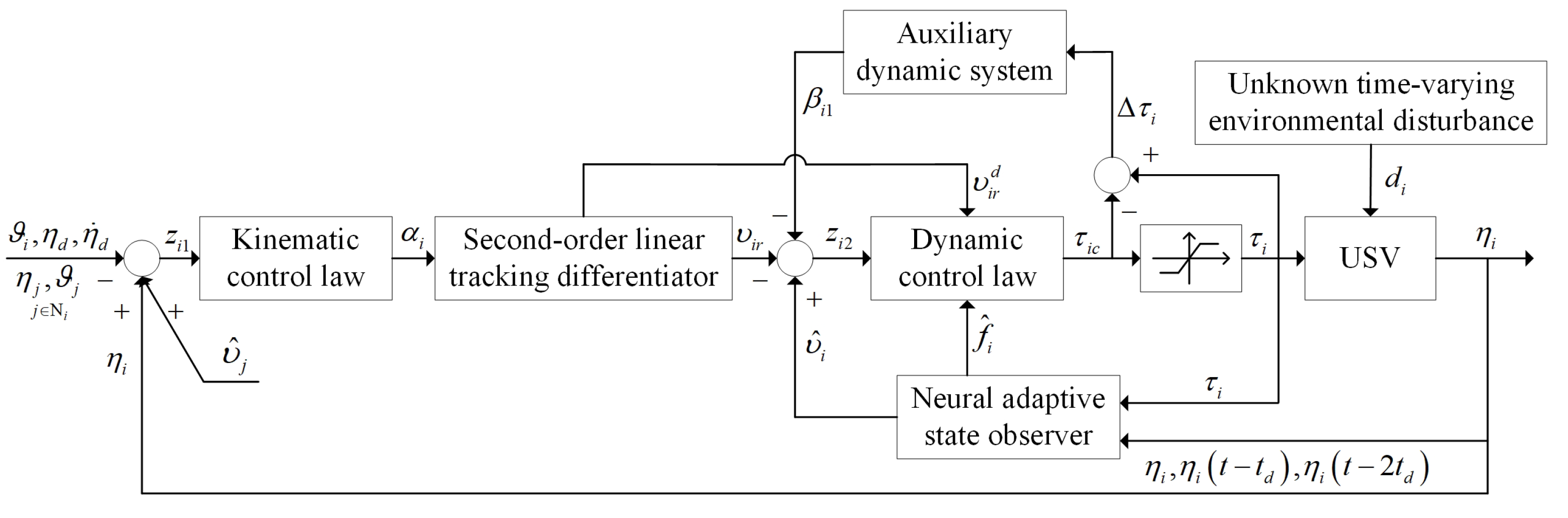
- A neural adaptive state observer is designed to recover velocity information and to estimate composite disturbances including model uncertainty and time-varying environmental disturbances.
- An auxiliary dynamic system is introduced to deal with input saturation. A modified BLF is provided to achieve connectivity preservation, collision avoidance and swarm control.
- In combination with the observer, an output feedback controller is proposed for the follower USVs based on a second-order linear tracking differentiator, an adaptive law, a modified BLF and graph theory. Meanwhile, the stability of the closed-loop system is proved via Lyapunov theory.
2. Preliminaries and Mathematical Modeling
2.1. Algebraic Graph Theory
2.2. Barrier Lyapunov Function
2.3. Neural Network
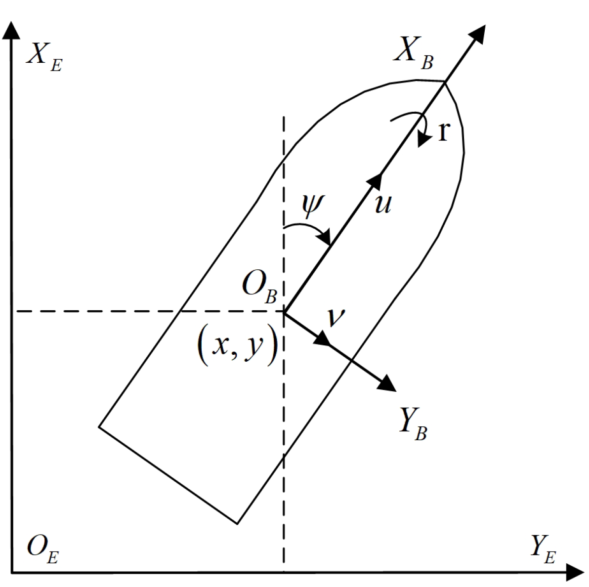
2.4. USVs Modeling
2.5. Environmental Disturbances Modeling
3. Neural Adaptive State Observer Design
4. Output Feedback Controller Design
4.1. Auxiliary Dynamic System
4.2. Output Feedback Controller Design
4.3. Stability Analysis
- (i)
- All signals in the closed-loop system are uniformly ultimately bounded.
- (ii)
- All USVs track the reference signal with a bounded tracking error.
- (iii)
- The output position of each USV satisfies output constraints.
5. Simulation Results
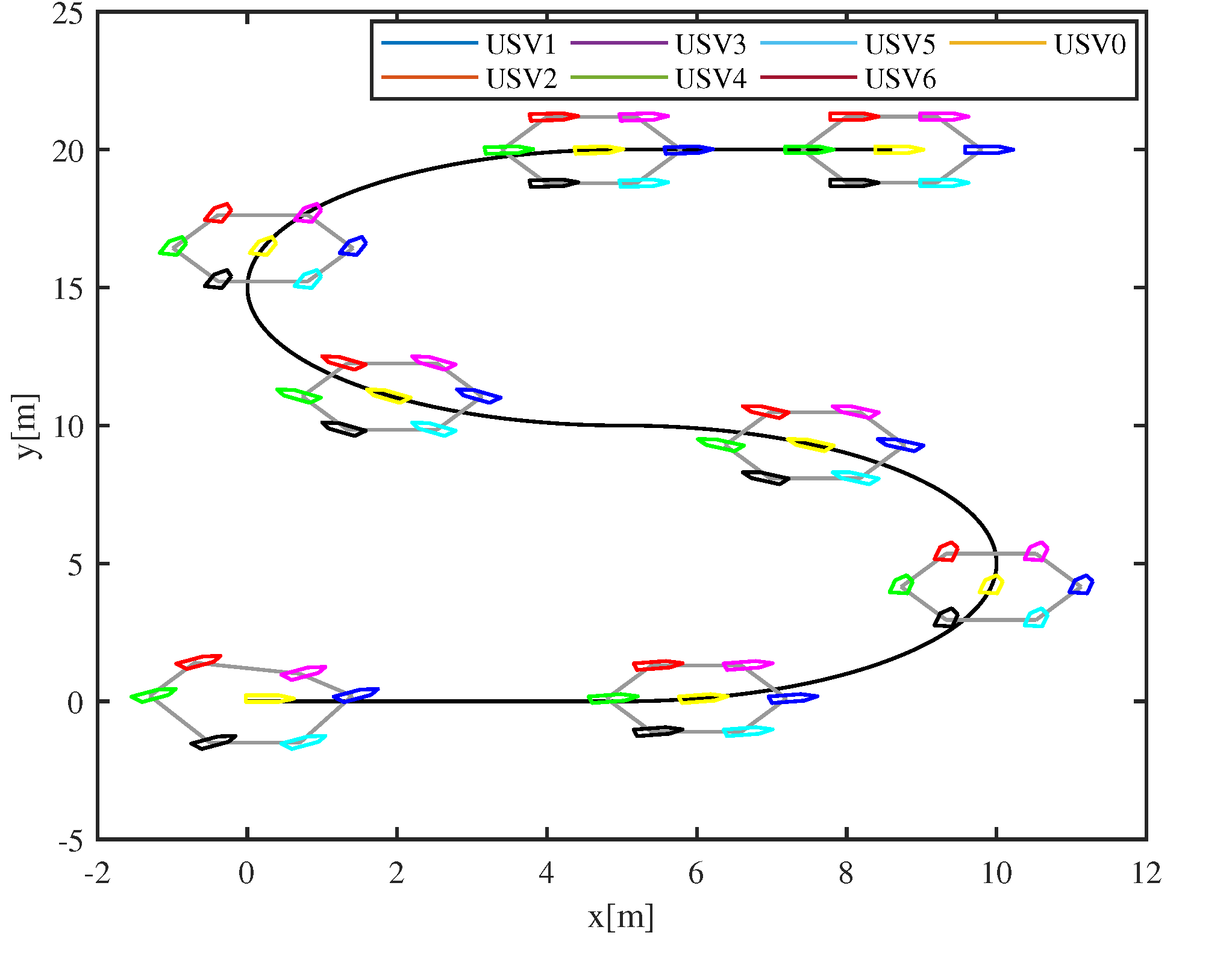
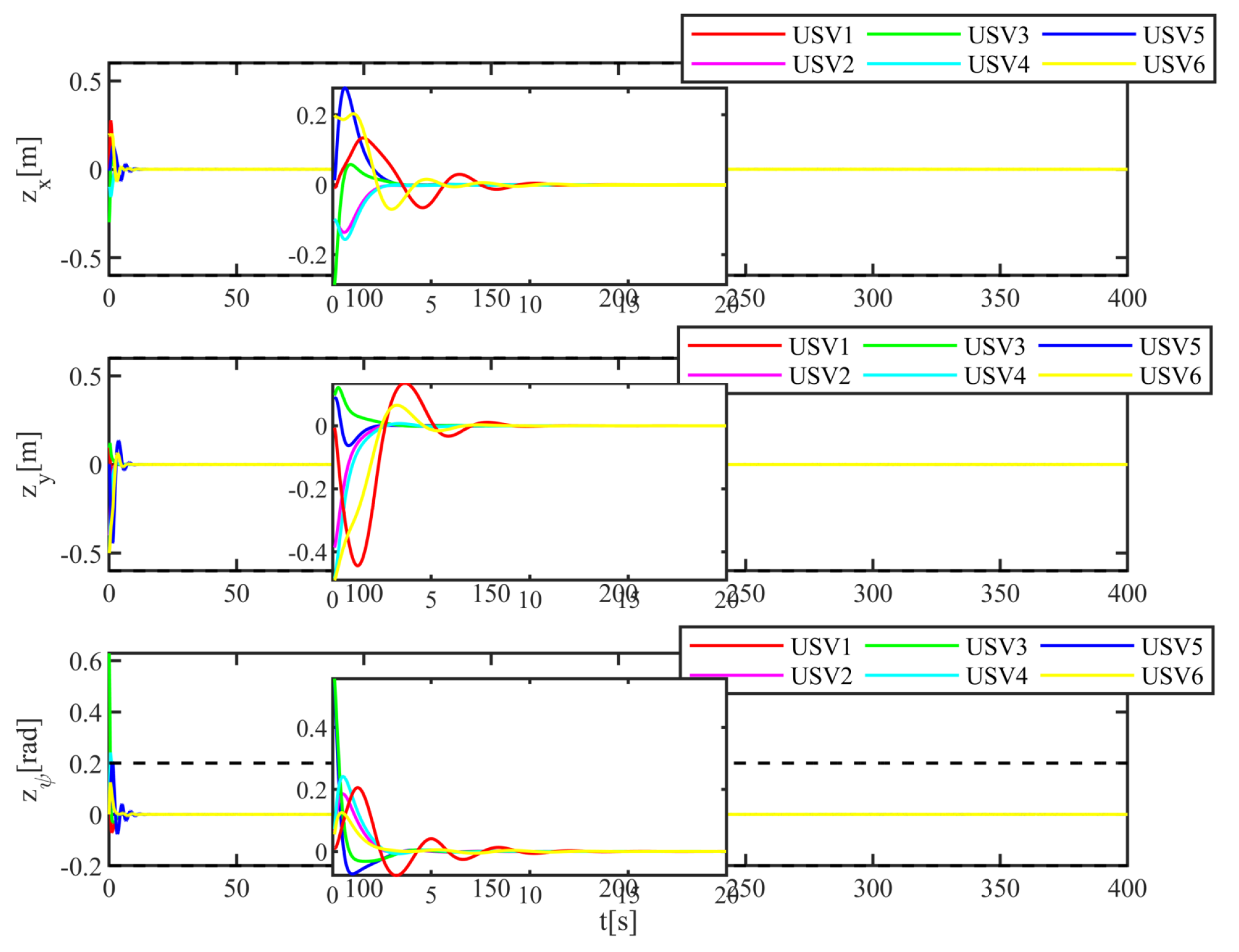
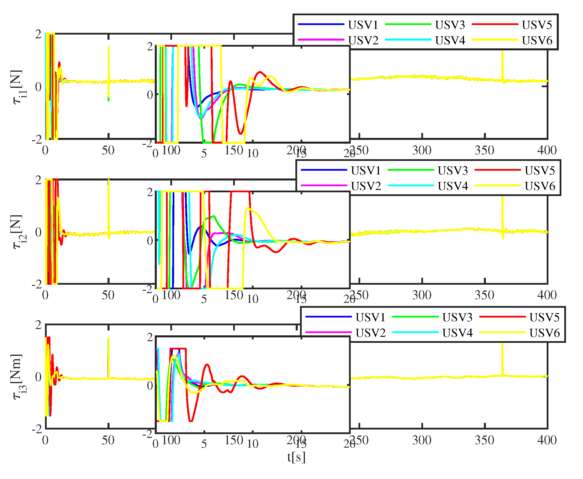
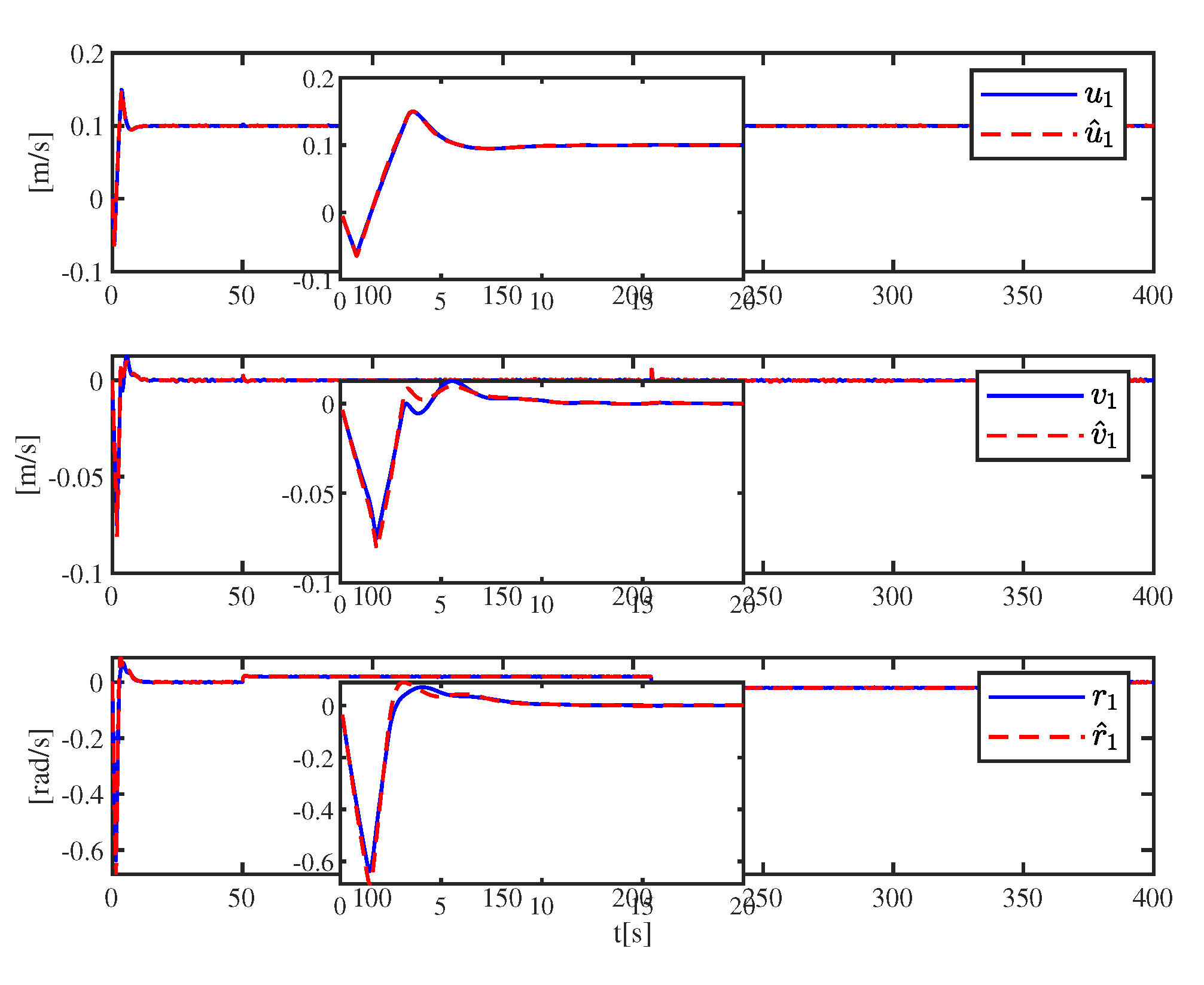
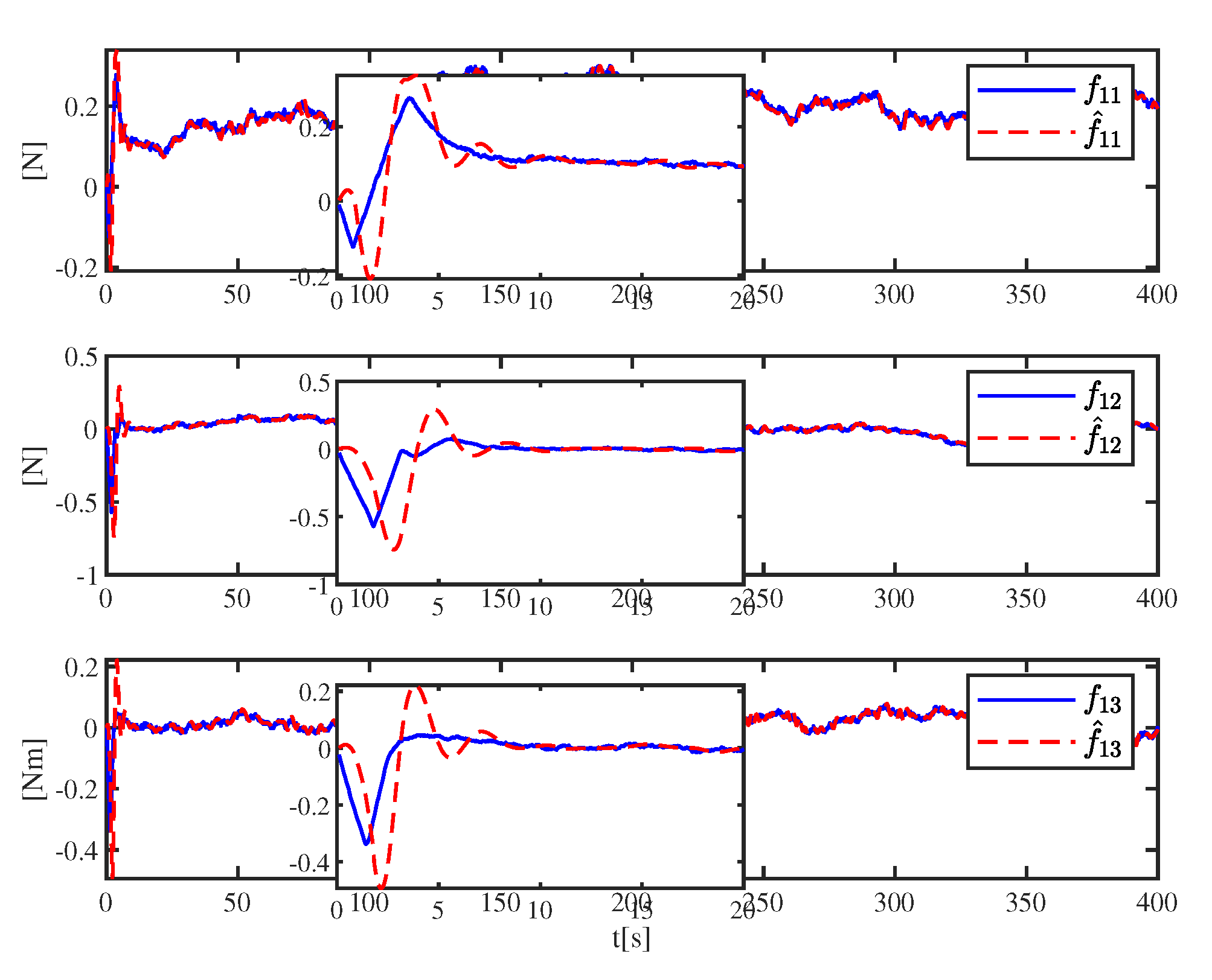
5.1. Performance of Proposed Control Strategy
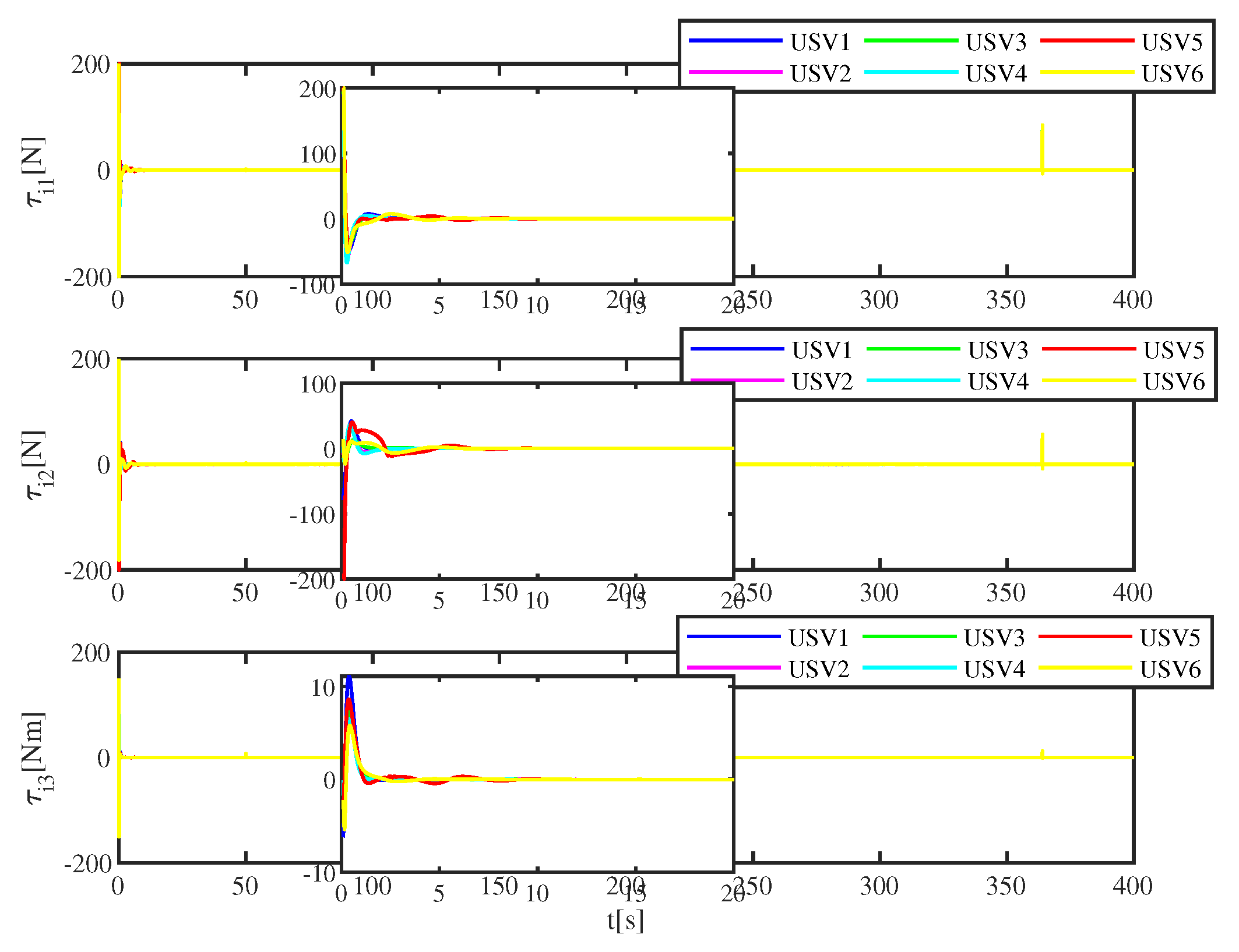
5.2. Comparison Group
6. Conclusions
Author Contributions
Funding
Institutional Review Board Statement
Informed Consent Statement
Data Availability Statement
Conflicts of Interest
Abbreviations
| USV | unmanned surface vehicle |
| BLF | barrier Lyapunov function |
| NN | neural network |
| NASO | neural adaptive state observer |
| LMIs | linear matrix inequalities |
| SOLTD | second-order linear tracking differentiator |
| ADS | auxiliary dynamic system |
| NADSC | neural adaptive dynamic surface control |
References
- Peng, Z.; Wang, J.; Wang, D. Distributed containment maneuvering of multiple marine vessels via neurodynamics-based output feedback. IEEE Trans. Ind. Electron. 2017, 64, 3831–3839. [Google Scholar] [CrossRef]
- Mahacek, P.; Kitts, C.A.; Mas, I. Dynamic Guarding of Marine Assets Through Cluster Control of Automated Surface Vessel Fleets. IEEE/ASME Trans. Mechatron. 2012, 17, 65–75. [Google Scholar] [CrossRef]
- Raboin, E.; Švec, P.; Nau, D.S.; Gupta, S.K. Model-predictive asset guarding by team of autonomous surface vehicles in environment with civilian boats. Auton. Robot. 2014, 38, 261–282. [Google Scholar] [CrossRef]
- Kim, Y.H.; Lee, S.W.; Yang, H.S.; Shell, D.A. Toward autonomous robotic containment booms: Visual servoing for robust inter-vehicle docking of surface vehicles. Intell. Serv. Robot. 2012, 5, 1–18. [Google Scholar] [CrossRef]
- Zoss, B.M.; Mateo, D.; Kuan, Y.K.; Tokić, G.; Ghamanbaz, M.; Goh, L.; Vallegra, F.; Bouffanais, R.; Yue, D.K.P. Distributed system of autonomous buoys for scalable deployment and monitoring of large waterbodies. Auton. Robot. 2018, 42, 1669–1689. [Google Scholar] [CrossRef]
- Chamanbaz, M.; Notarstefano, G.; Bouffanais, R. A randomized distributed ellipsoid algorithm for uncertain feasibility problems. In Proceedings of the 2017 IEEE 56th Annual Conference on Decision and Control, Melbourne, Australia, 12–15 December 2017; pp. 1305–1310. [Google Scholar]
- Zhang, L.J.; Jia, H.-M.; Qi, X. NNFFC-adaptive output feedback trajectory tracking control for a surface ship at high speed. Ocean. Eng. 2011, 38, 1430–1438. [Google Scholar] [CrossRef]
- Li, J.; Ren, W.; Xu, S. Distributed containment control with multiple dynamic leaders for double-integrator dynamics using only position measurements. IEEE Trans. Autom. Control 2012, 57, 1553–1559. [Google Scholar] [CrossRef]
- Ihle, I.A.F.; Skjetne, R.; Fossen, T.I. Output feedback control for maneuvering systems using observer backstepping. In Proceedings of the 13th Mediterranean Conference on Control and Automation, Limassol, Cyprus, 27–28 June 2005; pp. 1512–1517. [Google Scholar]
- Dai, S.L.; Wang, M.; Wang, C.; Li, L. Learning from adaptive neural network output feedback control of uncertain ocean surface ship dynamics. Int. J. Adapt. Control. Signal Process. 2014, 28, 341–365. [Google Scholar] [CrossRef]
- Wei, H.; Zhao, Y.; Sun, C. Adaptive Neural Network Control of a Marine Vessel With Constraints Using the Asymmetric Barrier Lyapunov Function. IEEE Trans. Cybern. 2017, 47, 1641–1651. [Google Scholar]
- Du, J.; Hu, X.; Liu, H.; Chen, C.L. Adaptive Robust Output Feedback Control for a Marine Dynamic Positioning System Based on a High-Gain Observer. IEEE Trans. Neural Netw. Learn. Syst. 2015, 26, 2775–2786. [Google Scholar] [CrossRef]
- Xia, G.; Shao, X.; Zhao, A. Robust Nonlinear Observer Furthermore, Observer-Backstepping Control Design For Surface Ships. Asian J. Control. 2015, 17, 1377–1393. [Google Scholar] [CrossRef]
- Zhang, J.; Yu, S.; Yan, Y. Fixed-time output feedback trajectory tracking control of marine surface vessels subject to unknown external disturbances and uncertainties. ISA Trans. 2019, 93, 145–155. [Google Scholar] [CrossRef]
- Li, X.; Shi, P.; Wang, Y. Distributed cooperative adaptive tracking control for heterogeneous systems with hybrid nonlinear dynamics. Nonlinear Dyn. 2018, 95, 2131–2141. [Google Scholar] [CrossRef]
- Xia, G.; Sun, C.; Zhao, B.; Xia, X.; Sun, X. Neuroadaptive Distributed Output Feedback Tracking Control for Multiple Marine Surface Vessels With Input and Output Constraints. IEEE Access 2019, 7, 123076–123085. [Google Scholar] [CrossRef]
- Peng, Z.; Wang, D.; Liu, H.H.T.; Sun, G.; Wang, H. Distributed robust state and output feedback controller designs for rendezvous of networked autonomous surface vehicles using neural networks. Neurocomputing 2013, 115, 130–141. [Google Scholar] [CrossRef]
- Lin, X.; Wang, Y.; Liu, Y. Neural-network-based robust terminal sliding-mode control of quadrotor. Asian J. Control 2022, 24, 427–438. [Google Scholar] [CrossRef]
- Yan, Z.; Wang, M.; Xu, J. Global adaptive neural network control of underactuated autonomous underwater vehilces with parametric modeling uncertainty. Asian J. Control 2019, 21, 1342–1354. [Google Scholar] [CrossRef]
- Seshagiri, S.; Khalil, H.K. Output feedback control of nonlinear systems using RBF neural networks. IEEE Trans. Neural Netw. 2000, 11, 69–79. [Google Scholar] [CrossRef] [Green Version]
- Lu, Y.; Zhang, G.; Sun, Z.; Zhang, W. Adaptive cooperative formation control of autonomous surface vessels with uncertain dynamics and external disturbances. Ocean Eng. 2018, 167, 36–44. [Google Scholar] [CrossRef]
- Tee, K.P.; Ge, S.S. Control of fully actuated ocean surface vessels using a class of feedforward approximators. IEEE Trans. Control. Syst. Technol. 2006, 14, 750–756. [Google Scholar] [CrossRef]
- Kahveci, N.E.; Ioannou, P.A. Adaptive steering control for uncertain ship dynamics and stability analysis. Automatica 2013, 49, 685–697. [Google Scholar] [CrossRef]
- Chen, M.; Tao, G.; Jiang, B. Dynamic Surface Control Using Neural Networks for a Class of Uncertain Nonlinear Systems With Input Saturation. IEEE Trans. Neural Netw. Learn. Syst. 2015, 29, 2086–2097. [Google Scholar] [CrossRef] [PubMed]
- Huang, B.; Song, S.; Zhu, C.; Li, J.; Zhou, B. Finite-time distributed formation control for multiple unmanned surface vehicles with input saturation. Ocean Eng. 2021, 233, 109158. [Google Scholar] [CrossRef]
- Zhou, W.; Wang, Y.; Ahn, C.K.; Cheng, J.; Chen, C. Adaptive Fuzzy Backstepping-Based Formation Control of Unmanned Surface Vehicles With Unknown Model Nonlinearity and Actuator Saturation. IEEE Trans. Veh. Technol. 2020, 69, 14749–14764. [Google Scholar] [CrossRef]
- Xia, G.; Xia, X.; Zhao, B.; Sun, C.; Sun, X. Distributed Tracking Control for Connectivity-Preserving and Collision-Avoiding Formation Tracking of Underactuated Surface Vessels with Input Saturation. Appl. Sci. 2020, 10, 3372. [Google Scholar] [CrossRef]
- Do, K.D. Formation Tracking Control of Unicycle-Type Mobile Robots With Limited Sensing Ranges. IEEE Trans. Control. Syst. Technol. 2008, 16, 527–538. [Google Scholar] [CrossRef] [Green Version]
- Do, K.D. Practical formation control of multiple underactuated ships with limited sensing ranges. Robot. Auton. Syst. 2011, 59, 457–471. [Google Scholar] [CrossRef]
- Hu, H.; Yoon, S.Y.; Lin, Z. Coordinated Control of Wheeled Vehicles in the Presence of a Large Communication Delay Through a Potential Functional Approach. IEEE Trans. Intell. Transp. Syst. 2014, 15, 2261–2272. [Google Scholar] [CrossRef]
- Yoo, S.J.; Kim, T.-H. Distributed formation tracking of networked mobile robots under unknown slippage effects. Automatica 2015, 54, 100–106. [Google Scholar] [CrossRef]
- Huang, Y.; Ding, H.; Zhang, Y.; Wang, H.; Cao, D.; Xu, N.; Hu, C. A Motion Planning and Tracking Framework for Autonomous Vehicles Based on Artificial Potential Field Elaborated Resistance Network Approach. IEEE Trans. Ind. Electron. 2020, 67, 1376–1386. [Google Scholar] [CrossRef]
- Tee, K.P.; Ge, S.S. Control of nonlinear systems with partial state constraints using a barrier Lyapunov function. Int. J. Control 2011, 84, 2008–2023. [Google Scholar] [CrossRef]
- Ghommam, J.; Saad, M. Adaptive Leader–Follower Formation Control of Underactuated Surface Vessels Under Asymmetric Range and Bearing Constraints. IEEE Trans. Veh. Technol. 2018, 67, 852–865. [Google Scholar] [CrossRef]
- Park, B.S.; Yoo, S.J. An Error Transformation Approach for Connectivity-Preserving and Collision-Avoiding Formation Tracking of Networked Uncertain Underactuated Surface Vessels. IEEE Trans. Cybern. 2019, 49, 2955–2966. [Google Scholar] [CrossRef]
- Yu, J.; Zhao, L.; Yu, H.; Lin, C. Barrier Lyapunov functions-based command filtered output feedback control for full-state constrained nonlinear systems. Automatica 2019, 105, 71–79. [Google Scholar] [CrossRef]
- Zhang, X.; Liu, L.; Feng, G. Leader–follower consensus of time-varying nonlinear multi-agent systems. Automatica 2015, 52, 8–14. [Google Scholar] [CrossRef]
- Liu, Y.; Lu, S.; Tong, S.; Chen, X.; Chen, C.L.P.; Li, D. Adaptive control-based Barrier Lyapunov Functions for a class of stochastic nonlinear systems with full state constraints. Automatica 2018, 87, 83–93. [Google Scholar] [CrossRef]
- Fossen, T.I.; Strand, J.P. Passive nonlinear observer design for ships using Lyapunov methods: Full-Scale experiments with a supply vessel. Automatica 1999, 35, 3–16. [Google Scholar] [CrossRef]
- Fossen, T.I. How to incorporate wind, waves and ocean currents in the marine craft equations of motion. In Proceedings of the 9th IFAC Conference on Manoeuvring and Control of Marine Craft, Arenzano, Italy, 19–21 September 2012; pp. 126–131. [Google Scholar]
- Park, B.S.; Yoo, S.J.; Park, J.B.; Choi, Y.H. Adaptive neural sliding mode control of nonholonomic wheeled mobile robots with model uncertainty. IEEE Trans. Control. Syst. Technol. 2009, 17, 207–214. [Google Scholar] [CrossRef]
- Skjetne, R.; Kokotović, P.V. Adaptive maneuvering, with experiments, for a model ship in a marine control laboratory. Automatica 2005, 41, 289–298. [Google Scholar] [CrossRef]


| Variable | Definition |
|---|---|
| Set of elements belonging to but not belonging to | |
| Absolute value of a scalar | |
| Euclidean norm | |
| dimensional Euclidean space | |
| Transpose of a matrix | |
| Inverse of a matrix | |
| ⊗ | Kronecker product of matrix |
| Adjacency matrix defined as with | |
| Defined as | |
| Degree matrix defined as diag | |
| diag | A block-diagonal matrix with being the ith diagonal element |
| Laplacian matrix defined as | |
| Information exchange matrix defined as | |
| Minimum of eigenvalues of a matrix | |
| Maximum of eigenvalues of a matrix | |
| dimensional identity matrix | |
| dimensional zero matrix |
| Parameters/ | Parameters/ | ||
|---|---|---|---|
Publisher’s Note: MDPI stays neutral with regard to jurisdictional claims in published maps and institutional affiliations. |
© 2022 by the authors. Licensee MDPI, Basel, Switzerland. This article is an open access article distributed under the terms and conditions of the Creative Commons Attribution (CC BY) license (https://creativecommons.org/licenses/by/4.0/).
Share and Cite
Xia, G.; Sun, X.; Xia, X. Swarm Control for Connectivity-Preserving and Collision-Avoiding Unmanned Surface Vehicles Subject to Multiple Constraints. J. Mar. Sci. Eng. 2022, 10, 827. https://doi.org/10.3390/jmse10060827
Xia G, Sun X, Xia X. Swarm Control for Connectivity-Preserving and Collision-Avoiding Unmanned Surface Vehicles Subject to Multiple Constraints. Journal of Marine Science and Engineering. 2022; 10(6):827. https://doi.org/10.3390/jmse10060827
Chicago/Turabian StyleXia, Guoqing, Xianxin Sun, and Xiaoming Xia. 2022. "Swarm Control for Connectivity-Preserving and Collision-Avoiding Unmanned Surface Vehicles Subject to Multiple Constraints" Journal of Marine Science and Engineering 10, no. 6: 827. https://doi.org/10.3390/jmse10060827
APA StyleXia, G., Sun, X., & Xia, X. (2022). Swarm Control for Connectivity-Preserving and Collision-Avoiding Unmanned Surface Vehicles Subject to Multiple Constraints. Journal of Marine Science and Engineering, 10(6), 827. https://doi.org/10.3390/jmse10060827