Many-Objective Container Stowage Optimization Based on Improved NSGA-III

Abstract

The container ship stowage planning problem (CSPP) is a very complex and challenging issue concerning the interests of shipping companies and ports. This article has developed a many-objective CSPP solution that optimizes ship stability and reduces the number of shifts over the whole route while at the same time considering realistic constraints such as the physical structure of the ship and the layout of the container yard. Use the initial metacentric height (GM) along with the ship’s heeling angle and trim to measure its stability. Meanwhile, use the total amount of relocation in the container terminal yard, the voluntary shift in the container ship’s bay, and the necessary shift of the future unloading port to measure the number of shifts on the whole route. This article proposes a variant of the nondominated sorting genetic algorithm III (NSGA-III) combined with local search components to solve this problem. The algorithm can produce a set of non-dominated solutions, then decision-makers can choose the best practical implementation based on their experience and preferences. After carrying out a large number of experiments on 48 examples, our calculation results show that the algorithm is effective compared with NSGA-II and random weighted genetic algorithms, especially when applied to solve many-objective CSPPs.

1. Introduction

The container ship stowage planning problem (CSPP) determines the specific location of a container on a ship. As an essential part of maritime container transportation, the CSPP is one of the problems that container terminals and shipping companies must face and solve every day [1,2]. The quality of stowage determines the safety and seaworthiness of a ship, which directly affects the berthing time of vessels and indirectly affects transportation efficiency. In addition, the quality of stowage is closely related to the shipping company’s efficiency and the cargo owner’s vital interests. When making a container stowage plan, the following aspects must be considered [3,4,5].

First, the seaworthiness and proper stability of the ship must be ensured. Because there are many containers on the deck, and the number of containers on the deck may even exceed the number of containers in the hold, container ships are different from other ship types. Container ships are prone to the characteristics of a sizeable wind-receiving area and a high center of gravity. During the whole process of loading and unloading and the entire process of sailing, it is necessary to ensure a certain initial metacentric height (GM), appropriate trim, and timely adjustments to the ship’s heeling, as well as to consider the influence of the blind area of the bridge’s sight. The initial metacentric height is significant for the navigation of ships, and at the same time represents a “sensitive” constraint. If its value is too small, the ship is prone to capsizing. Especially as the ship becomes larger and faster, the economic pressure of navigation in severe weather will tend to increase, thus increasing the risk of capsizing [6]. A too-large value will shorten the rolling period, aggravate hull shaking, reduce crew comfort, and increase the lashing rope’s risk of loosening. In [7], ship stability is regarded as a mandatory constraint. The ship’s operator can use ballast water to adjust non-critical stability issues [8]; however, a good stowage plan needs to optimize the use of ballast water to reduce the ship’s trim in order to improve fuel efficiency.

Second, the limitations imposed by the physical structure of the containers must be met. Both the loading and unloading of containers follow the LIFO (last in, first out) policy [9]. Special containers such as reefer containers, dangerous goods containers, and oversized containers have specific storage requirements. Due to corn fittings at the bottom, two 20-ft containers cannot stack on a 40-ft container.

Third, the container ship’s hull must have sufficient strength. Measures of the strength of a container ship’s hull includes shear force, transverse strength, torsional strength, local strength, and longitudinal strength. In loading, unloading, and transportation, stowage planning must meet the hull’s strength and safety requirements and extend the ship’s service life.

Fourth, the number of container shifts should be minimized. There are many ports of call and the loading and unloading of midway ports are more frequent, especially for transoceanic and global container liners. For this reason, when planning stowage an overall view of the whole route should be taken that carefully considers the order in which ships call and the information provided by each port of call. Earlier ports must be considered when planning for later ports. The starting port should lay the foundation for the entire route to avoid the situation of containers meant for earlier ports being blocked by those meant for later ports. Otherwise, container shifting will reduce the efficiency of loading and unloading, extend the turnaround time, and increase the cost. In addition, relocation will incur expensive additional loading and unloading costs (usually, a single loading and unloading costs tens to hundreds of US dollars) [10,11].

Finally, excessive concentration of containers in the same port of discharge is to be avoided. The makespan of quay cranes directly affects a ship’s turnaround time and port costs. Usually, two or more cranes simultaneously speed up the discharge process for large container ships [12]. However, the quay crane cannot simultaneously lift the containers in two adjacent spaces on the container ship. In the case of the above situation, containers intended for the same discharge port should not be arranged in adjacent holds.

Based on the above discussion, the following two goals are crucial in container stowage.

(a)

Ensure proper stability and trim of the ship;

(b)

Minimize the amount of container relocation on the whole route.

Goal (a) relates to the safety of ships, while goal (b) relates to the profit and efficiency of shipping companies and port terminals. While each has its own merits, in actual operation there are often conflicts. For example, reducing the number of container shifts may come at the cost of reducing the ship’s stability. In engineering applications, this type of combinatorial optimization problem is called a multi-objective CSPP (MO-CSPP). In our research, the number of objectives exceeds three (i.e., six); thus, it is a many-objective CSPP (MaO-CSPP). As a remarkably realistic engineering problem in container transportation, MaO-CSPP has attracted the attention of more and more scholars. Multi-objective optimization is a common type of optimization decision-making problem which has been applied in many fields. The optimal solution is usually based on the trade-off between two or more conflicting objectives. To solve an MaO-CSPP according to different decision-making methods, two methods are typically used, namely, the a priori and a posteriori techniques [13].

The a priori technique represents the basic idea behind solving multi-objective optimization problems in traditional mathematical programming. Before searching, the decision information is input and one solution is run to the decision-maker. The main methods include lexicographical, linear fitness, and nonlinear fitness methods. The objective functions of the MaO-CSSP are aggregated to obtain a single-objective optimization problem. Then, the single-objective optimization method is used to obtain a single Pareto-optimal solution. While the idea of this method is simple, in practical engineering applications it is difficult to determine the weighting preferences between the objectives. In MaO-CSPP, the stability and strength of the ship must be guaranteed within a specific range. However, it is difficult to determine the respective weights of the amount of container relocation and the ship’s stability and strength from the perspective of economic profit. Therefore, the priori technique is sometimes not suitable for solving MaO-CSPPs in this context.

In contrast, running the a posteriori technique generates solutions for decision-makers to choose from. This technique generates a representative subset of the global or local Pareto-optimal solutions. If at least one of its goals is not inferior to other solutions in the solution space, the solution is Pareto optimal. If it is not dominated by any other solutions in the solution space, it is Pareto optimal [14]. Domination-based multi-objective optimization has been proven to be suitable for MaO-CSPPs.

A set of Pareto-optimal solutions can be obtained in a single run without prior information by using the a posteriori technique. Decision-makers can then weigh different goals and choose an ideal solution for actual implementation. The above studies on CSPPs seldom consider the principles of ship stability, strength, draught, etc., as they are conducted from a purely mathematical point of view and the yard optimization problem is not included. At the same time, most of the literature does not incorporate the characteristics of the full-route ports of call, instead using only a single port to design the stowage plan. On this basis, the present paper proposes a many-objective method that weighs safety and economic benefits from the perspective of both ship and port, and thereby enriches the research content regarding CSPPs. The rest of this article is organized as follows. In Part Two, a literature review is provided summarizing the latest progress on CSPPs and multi-objective evolutionary optimization algorithms; in Part Three, we introduce the CSPP; in Part Four, we present an algorithm that combines local search and genetic operators, and provide specific details to solve the problems raised in Part Three; in Part Five describes the many examples and experiments we conducted; finally, Part Six contains our conclusions along with prospects for future research.

2. Literature Review

CSPP is occasionally referred to as the master bay plan problem (MBPP) or ship stowage planning problem (SSPP) [15]. In 1970, Webster and Van Dyke first studied CSPP [16]. As their research only discussed simple issues, and did not conduct many experimental data tests, it is impossible to demonstrate the practical significance of their methods. Subsequently, in the 1980s Shields proposed the CAPS system (computer-aided pre-planning system) and applied it to the American President Line (APL) [17]; this system uses Monte Carlo stochastic simulation technology to generate different stowage plans. Avriel et al., proved that the CSSP is an NP-hard problem and demonstrated its relationship with the graph coloring problem [15], then established a 0–1 mathematical programming model and designed a “Suspensory Heuristic Procedure” in which the optimal solution for the small-scale stowage plan is automatically generated [18]. Ambrosino et al., attempted to derive rules that determine a good stowage plan [19]. The authors define and characterize the feasible solution space by satisfying certain constraints. The 0–1 linear programming model was then established to solve this combined optimization problem [20,21] using rules to develop a heuristic algorithm in which containers that have the same attribute should be placed in the same hold. However, the paper does not explicitly consider the issue of relocation related to the loading process. The authors expanded the original basic model by considering the influence of different container types (i.e., 20-ft and 40-ft containers) [22,23]. Imai et al., established an integer programming model intended to minimize the shift volume of the yard and the ship’s stability. However, the model did not consider the impact of hatch covers on stowage [8]. It is difficult to estimate the number of shifts when the information left by the container truck is uncertain as to storage space. Therefore, Imai proposed an estimate of the expected number of shifts [24]. Li et al., established a 0–1 mathematical programming model [25] by maximizing container ship hold utilization while minimizing operating costs over the whole route. Cruz-Reyes et al., developed 0/1 IP and employed a constructive heuristic to find the solution [26]. Petering et al., introduced a new mathematical formula for the block relocation problem by establishing an integer programming model. This method has been proven to produce fewer decision variables and better performance [27]. N. Wang et al., established an integer programming model and solved it with a CPLEX solver [28]. Fan et al., designed an effective algorithm to solve the optimization problem of the container stowage plan while considering many practical and operational constraints. However, no specific mathematical model has been set up to describe the optimization of container stowage plans [29].

All of the above-mentioned literature relies on traditional mathematical programming methods to deal with the problem of container stowage; this is only suitable for small-scale situations, and most applications are single-bay container stowage problems [30], which do not have practical engineering significance. Therefore, scholars often adopt a multi-stage method when facing actual scale problems, i.e., the CSPP is decomposed into sub-problems that are easier to handle. The corresponding sub-problems are then dealt with separately, and the solutions of the sub-problems are spliced to obtain a solution. In addition, Monaco introduced a systematic classification scheme for CSPP [31]. Wilson et al., designed a two-stage process for a container stowage plan in which the first stage is a global stowage strategy and the second stage is a partial stowage strategy [32]. Kang and Kim decomposed the container stowage problem into two sub-problems. The first sub-problem allocates containers to different countermeasure holds, and the second sub-problem determines the specific placement of containers in each hold [33]. Ambrosino et al., described the problem as an optimization problem [22]. They defined the problem as a master bay plan problem (MBPP). In response to this problem, the author proposed a three-stage heuristic model to deal with the sub-problems of each stage separately and developed a basic 0–1 linear programming model to minimize the total loading time. The subsequent literature [23] expanded the work of [22] and achieved specific results. Based on their consideration of structural and operational constraints, Ambrosino et al., proposed a multi-port MBPP heuristic algorithm based on MIP to minimize ship berthing time [34]. Later, they offered an MIP model to minimize the number of reprocessing and crane makespan which took into account such realistic constraints as six ports of call and both standard containers and reefer containers [35]. In a recent study, the authors used a specific stowage principle to solve the CSPP in the presence of dangerous containers [36]. Delgado et al., decomposed the ship stowage plan into two sub-problems, the main stowage plan and the location plan, using the calculation result of the main stowage plan as the input data of the location plan [30]. Pacino et al., proposed a two-stage method for large container ships; the first stage deals with the multi-port main bay stowage plan and the second stage uses the constraint programming (CP) method and slot planning to allocate specific slots for each container [37]. Iris Ç et al., presented a flexible container ship loading problem for seaport container terminals. They integrated the assignment and scheduling of transfer vehicles and container load sequencing with the assignment of specific containers to specific vessel positions [38]. Gumus et al., developed a multi-stage heuristic of the CSPP by decomposing the problem into four stages, explaining many complex and realistic CSPPs [39]. Zhang et al., deteriorated the full-route container stowage problem into a bay selection sub-problem and a slot plan sub-problem. The second sub-problem was then further subdivided into single destination port and a multi-destination port bay position optimization problem [40]. Azevedo et al., studied the optimization of container stowage plans considering the operation of quay cranes, taking additional practical and operational constraints into account, and designed a new solution method to solve the problem. However, the related characteristics of the container crane and the container were simplified without considering different container weights and sizes or the additional productivity of the quay crane [41]. Christensen et al., extended the liner shipping cargo mix problem by including the concepts of block stowage and draft restrictions and restricting the number of containers able to be selected, with the aim of determining the optimal cargo mix, not of creating a fully feasible stowage plan. Instead of assigning specific containers to specific slots on the vessel, containers are grouped by container type and assigned to blocks. Each container type represents several containers with the same properties [42]. Yaagoubi et al., studied 3D container loading planning of inland navigation barges. They proposed a heuristic method based on the first fitting algorithm of the packing problem, which is able to deal with actual structural and operational constraints [43]. According to inland container liner transportation characteristics, Li et al., decomposed the current port stowage planning problem into two sub-problems and proposed two heuristic algorithms for them [44]. Iris et al., systematically reviewed the literature related to stowage planning, loading sequencing, and scheduling. From the perspective of the ship loading problem (SLP), the authors pointed out that the literature on integration efforts for the SLP was rather limited, that is, most literature focuses on optimizing partial SLP issues. These studies have contributed to solving the SLP by proposing new models or algorithms to find improved solutions to various aspects of the SLP [45].

To enhance the practicality of the algorithm, scholars have gradually begun to apply heuristic or meta-heuristic methods to the field of ship stowage. Avriel et al., developed a Suspensory Heuristic Procedure to process CSPP that minimizes the number of container shifts without considering stability or strength [18]. Based on [18], Ding extended and enriched the Suspensory Heuristic Procedure [46]. Dubrovsky et al., proposed compact coding technology to design a genetic algorithm (GA) suitable for the CSPP. The significant feature of this method is that it reduces the number of iterations [47]. Jin et al., established an MIP model based on reality constraints, proposed an interactive hybrid algorithm consisting of a combination of a heuristic algorithm and a GA based on a pre-allocation strategy, and realized the visualization of stowage plans using the VB program [48]. Sciomachen and Tanfani considered this model’s structural and operational constraints as they relate to containers and ships. They proposed a heuristic method that uses the relationship between MBPP and the three-dimensional packing problem to solve the MBPP problem [49]. Parreño proposed a greedy randomized adaptive search procedure (GRASP) to solve the problem of container stowage slot planning [3]. Similarly, they studied multi-port CSPP and proposed an IP model and a GRASP algorithm, generating a stowage plan with the smallest number of container shifts for large-scale problems [50]. Araújo et al., proposed a Pareto clustering search algorithm to solve the double objective optimization model of container stowage (with the objectives of the number of movements necessary to load and unload the container ship and the stability of the ship in each port), designed a heuristic algorithm, grouped clustering through local search, and found the Pareto frontier to obtain the effective solution of the problem [51]. Zhang studied a multi-objective CSPP, seeking to optimize the stability of the ship and the number of containers to be reprocessed at the same time. The author developed multiple heuristic algorithms to deal with both containers in the yard and containers in the bay of ships, then integrated these heuristic algorithms into a non-dominated sorting GA [52]. Wilson and Roach used Tabu Search (TS) to generate CSPP solutions, and found that TS can gradually improve the location of containers [53]. Yurtseven implemented two meta-heuristic algorithms, namely, GA and simulated annealing (SA), to solve the CSPP. Their results show that SA can reach near-optimal results faster than GA [54]. Ambrosino et al., tested the performance of three methods to solve the MBBP, i.e., TS, a simple heuristic algorithm, and an ant-colony optimization (ACO) algorithm. Their results show that ACO is the best for large-scale instances, while TS is ideal for medium-sized cases [23]. Bilican et al., proposed a two-stage heuristic solution method using IP and a swapping heuristic (SH), which effectively increases the scale of solvable problems [6]. Junqueira et al., proposed an optimization model that combines the multi-port stowage planning problem with the container relocation problem. The author presented two heuristic methods to quickly generate feasible solutions [55]. Ji et al., established a mixed-integer nonlinear programming model based on small feeder container ships’ “sensitive” characteristics to ensure navigation safety. The authors designed a heuristic algorithm to update branch routes through variable neighborhood search and GA in order to obtain the stowage plan [56].

Although the literature mentioned above discusses several objectives of CSPP, most studies treat the CSPP as a single-objective optimization problem; there are few studies on the MO-CSPP or MaO-CSPP. Imai et al., considered two criteria with respect to the MO-CSSP, namely, ship stability and the number of rehandlings [8]. However, they used a weighted sum method and designed a GA to handle single-objective CSSPs. Liu et al., considered five objectives, i.e., the number of container shifts, the quay cranes’ makespan, the number of stacks exceeding the weight limit, the number of stacks without containers, longitudinal stability, and transverse stability, then developed a random algorithm incorporating TS to find a set of Pareto-optimal solutions [57].

In 1989, David Goldberg proposed using evolutionary algorithms (EA) to achieve multi-objective optimization technology. Multi-objective evolutionary algorithms (MOEA) have subsequently attracted widespread attention from many researchers, and many research results have emerged. When solving MO-CSSPs, to the best of our knowledge only Zhang et al., have used the MOEA [52]. This paper proposes to use the concept of Pareto optimality according to the idea of non-dominated sorting to produce a set of solutions for decision-makers.

3. Problem Description

3.1. Arrangement and Layout of the Slot

Three longitudinal, horizontal, and vertical parameters are required to define a slot. The internationally unified slot code numbering method formulated by ISO is adopted. It is based on the premise that the containers are distributed longitudinally on the ship. Six digits represent the coordinates of each slot. The first two digits are ”Bay No.”, the middle two digits are “Row No.”, and the last two digits are ”Tier No.” From bow to stern, the cargo hold of a container ship is longitudinally divided into several 20-foot-long areas. Usually, two adjacent 20-foot container slots form a 40-foot container slot. Certain holds are equipped with detachable cell guides. The hold can only be used as a 20-foot container when the cell guides are installed, and can only be used as a 40-foot container when the cell guides are removed.

Container ships are complex structures, and each voyage has a different bay layout. To simplify the problem, we put forward the following assumptions.

• The information on the containers to be loaded in each port of call of this voyage is known before stowage, including the port of loading, the port of discharge, and the cargo type, quantity, weight, etc.
• We only consider standard containers. Reefers, dangerous containers, or other non-standard container types have a particular hold on a ship, and this article does not study them.
• Our research only focuses on 20-foot containers and does not consider the mixed loading of 20-foot and 40-foot containers.
• We abstract the bay position of the ship as a similar rectangular shape, i.e., the number of rows of each bay position is equal, denoted by r_S. The number of bays on the ship is represented by b_S, and it is assumed that the maximum height of each bay is t_S. Irregular forms can be expressed by adding constraints. Our current study does not consider the influence of hatch covers, i.e., it does not distinguish between hold and deck.
• The structure of the yard bay is similar to the design of the ship hold. Similarly, the yard bays, the number of rows of each bay, and the number of layers of each row are represented by r_Y, b_Y, and t_Y, respectively.

3.2. Stability Check

Stability can be divided into transverse stability and longitudinal stability, according to the inclination direction. The leading indicators of the former are initial transverse metacentric height (GM) and heel (θ) [58]; the trim mainly measures the latter. As shown in Figure 1 [59], from the respective relative positions the GM can be expressed as

$$GM=KM-KG$$

(1)

where KM denotes the height from the metacenter point M to the baseline and KG denotes the height from center of gravity G to baseline.

After loading and unloading the container, the GM of the ship will change. For displacement of the ship after loading and unloading the container, the calculation process is as follows:

$${\Delta }_1=\Delta +{\displaystyle \sum P_i}$$

(2)

where Δ denotes the ship’s displacement before loading and unloading, Δ₁ denotes the ship’s displacement after loading and unloading, and P_i means the weight of the i-th container.

According to the theorem of resultant moments, find the coordinates of the ship’s center of gravity after loading and unloading the containers.

$$\begin{array}{c}{x}_{g1}=\frac{\Delta ·x_g+{\displaystyle \sum P_i{z}_i}}{{\Delta }_1}\\ y_{g1}=\frac{\Delta ·y_g+{\displaystyle \sum P_i{y}_i}}{{\Delta }_1}\\ x_{g1}=\frac{\Delta ·x_g+{\displaystyle \sum P_i{x}_i}}{{\Delta }_1}\end{array}$$

(3)

where (x_g,y_g,z_g) denotes the coordinates of the ship’s center of gravity before loading and unloading, (x_i,y_i,z_i) means the coordinate of the center of gravity of the i-th container, and (x_g1,y_g1,z_g1) denotes the coordinates of the ship’s center of gravity after loading and unloading.

According to the displacement of the ship after loading and unloading a container Δ₁, query hydrostatic data to obtain the mean draft (d₁), height of the ship’s metacenter from baseline (KM₁), moment to change trim 1 cm (MTC₁), longitudinal distance of the center of floatation (x_f), longitudinal distance of the center of buoyancy (x_b) above, and any other parameters.

If there are free surfaces, perform a free surface correction. The GM of the ship after loading and unloading is as follows:

$$G_1{M}_1=K{M}_1-x_{g1}-{\displaystyle \sum \frac{{\rho }_i{i}_x}{{\Delta }_1}}$$

(4)

where G₁M₁ denotes the GM of the ship after loading and unloading, ρ_i denotes the density of the i-th free surface liquid, and i_x indicates the inertial moment of the free surface on the inclined axis.

If y_g1 ≠ 0, the ship has a heel angle; the tangent value of the heel angle is expressed as follows:

$$\tan \theta =\frac{{\displaystyle \sum P_i}·y_{g1}}{{\Delta }_1·G_1{M}_1}$$

(5)

If x_g1 ≠ x_b1, the trim of the ship is as follows:

$$\delta t=\frac{{\Delta }_1·\left(x_{g1}-x_{b1}\right)}{100MT{C}_1}$$

(6)

In the actual stowage work, the G₁M₁ should be within an advisable range in order to maintain sufficient stability and obtain an appropriate roll period. Generally speaking, for a container ship with twelve rows of containers the G₁M₁ is about 1.0 m and the roll period is about 25 s. The heel angle, θ, should be minimized in order to obtain a better floating condition for the heel angle. When constraining the trim, the target should not be set as the minimum trim; rather, it should be set to a specific value, t₀, the calculation of which can be found in [60]. The paper “Trimming Optimization” shows that the optimum trim angle varies with ship speed and draft. In the actual operation process, because the relevant port usage fees of many ports are related to the maximum draft of ships arriving at the port all ships should try their best to keep an even keel when entering and leaving the port in order to reduce expenses.

3.3. Container Stowage Process

A container ship stowage plan for a whole route refers to the operation of a certain route, taking into consideration the loading and unloading ports of all containers to be loaded, determination of the specific positions of all containers to be loaded into the ship, and compiling of a ship stowage plan for each port [61]. Every voyage should as much as possible attempt to avoid or reduce the number of container shifts to ensure ship safety and achieve the goal of improving the efficiency of loading and unloading. A whole route can be subdivided into metro loop, cycloid, and hybrid type routes, as shown in

Table 1. Types of containership stowage plans for full routes.

Types	Metro Loop	Cycloid	Hybrid
Sketch
Cargo Flow

.

A container ship first unloads import containers at the current port, then loads that port’s export containers. Here, we assume that the loading and unloading processes are separate and that import containers are unloaded first, then export containers are loaded. Although there are situations where loading and unloading are carried out simultaneously at certain ports, the above assumption is in line with current yard operation realities.

The unloading operation of imported containers mainly involves the optimization of container stacking in the terminal yard, of the path of the straddle carrier, and of quay crane dispatching. As this research focuses on the impact of export container loading on ship stability and subsequent container shifts, the main focus of this article is on the export container loading process. After a container ship arrives at the port of call, the containers are unloaded at the port. The loading operation is based on the layout of the unloaded containers on the ship.

For the three types of full-route container ship stowage plans mentioned above (i.e., metro loop, cycloid, and hybrid type routes), when a ship arrives at a port of call and unloads its import containers there will be containers intended for subsequent ports on board the vessel. At this time, there the following three scenarios for shifting are in play. The first occurs in the export container yard. Due to the different times at which export containers arrive at the terminal yard and the other subsequent ports of call of the export containers, under the premise of a given loading sequence the containers will be relocated when the yard containers are retrieved. Extensive research has been carried out on the optimization problem of container relocation within the yard. Pre-marshaling [62] can effectively reduce the amount of container relocation when retrieving containers from the yard. In the second scenario, container relocation may occur on container ships in the current port. To reduce the amount of container relocation required at subsequent calls, the stacking order of containers on the ship will be reorganized in the current port; such relocations are called ‘voluntary shifts’. In the third scenario, if a container is considered a blocking container, it must be relocated in order to retrieve the container below it in the next port; these relocations are called ‘necessary shifts’.

The number of shifts corresponding to a given container loading plan is composed of the following three parts.

• As shown in Figure 2, given the loading sequence, the amount of relocation due to stacking yard turnover can be found in [63].
• As shown in Figure 3, the container is temporarily unloaded on the dock and then added to the subsequent loading sequence, that is, voluntary shifts. The literature on voluntary shifts mainly expands on and synthesizes [18,46].
• As shown in Figure 4, the amount of container relocation in subsequent ports are necessary shifts.

3.4. MaO-CSPP

To completely express the MaO-CSPP, it is necessary to clarify the optimization objective of the problem and the feasible solution under various constraints. As previously mentioned, the objectives for the MaO-CSPP can be divided into two categories, i.e., f₁ and f₂, where f₁ relates to stability and f₂ relates to the number of shifts; X is a feasible solution to the MaO-CSPP where $X=\left(x_1,x_2\cdots ,x_n\right)$ is a stowage plan that satisfies various constraints. The objective function of the MaO-CSPP with six optimization objectives, as studied in this paper, can be expressed as

$$f\left(X\right)=\left(\begin{array}{cccccc}{f}_{11}\left(X\right),& f_{12}\left(X\right),& f_{13}\left(X\right),& f_{21}\left(X\right),& f_{22}\left(X\right),& f_{23}\left(X\right)\end{array}\right)$$

(7)

where $\left\{f_{11},f_{12},f_{13}\right\}\in f_1$, $\left\{f_{21},f_{22},f_{23}\right\}\in f_2$. The specific meanings of the above six objective functions are shown in

Table 2. The specific meaning of the six objective functions of the MaO-CSPP.

Category	Objective	Range	Target
Stability ($f_1$)	Initial metacenter height ($f_{11}$)	$\left[0,+\infty \right)$	max$f_{11}\left(X\right)$
	Heel angle ($f_{12}$)	$\left(-\infty ,+\infty \right)$	min$\left|f_{12}\left(X\right)\right|$
	Trim value ($f_{13}$)	$\left(-\infty ,+\infty \right)$	min$\left|f_{13}\left(X\right)\right|$
Shifting ($f_2$)	relocation in the yard by yard cranes ($f_{21}$)	$\left[0,+\infty \right)$	min$f_{21}\left(X\right)$
	container voluntary shifts by quay cranes ($f_{22}$)	$\left[0,+\infty \right)$	min$f_{22}\left(X\right)$
	container necessary shifts at future ports ($f_{23}$)	$\left[0,+\infty \right)$	min$f_{23}\left(X\right)$

.

The MaO-CSPP can be described as

$$\min \begin{array}{c}\end{array}\left\{\begin{array}{cccccc}-f_{11}\left(X\right),& \left|f_{12}\left(X\right)\right|,& \left|f_{13}\left(X\right)\right|,& f_{21}\left(X\right),& f_{22}\left(X\right),& f_{23}\left(X\right)\end{array}\right\}$$

(8)

$$\mathrm{s}.\mathrm{t}.\begin{array}{c}\end{array}X\in \mathbb{X}$$

(9)

Equation (8) is called the objective function. For multi-objective functions, the a priori technique can be adopted. In the case of a given weight preference, the goals of the original multi-objective problem are aggregated in a linear or non-linear manner to obtain a single-objective optimization problem. Then, the single-objective optimization method is used to find a single Pareto-optimal solution, e.g., Equation (10):

$$\min \begin{array}{c}\end{array}{g}^{ws}\left(X|\lambda \right)={\lambda }_1\left(-f_{11}\left(X\right)\right)+{\lambda }_2\left|f_{12}\left(X\right)\right|+{\lambda }_3\left|f_{13}\left(X\right)\right|+{\lambda }_4{f}_{21}\left(X\right)+{\lambda }_5{f}_{22}\left(X\right)+{\lambda }_6{f}_{23}\left(X\right)$$

(10)

which satisfies ${\lambda }_i\ge 0$, $i=1,\cdots ,6$ and ${\displaystyle \sum _i{\lambda }_i}=1$.

In Equation (9), $\mathbb{X}$ is the feasible solution space. There are usually two ways of expressing the feasible solution of x, one of which uses MIP, which can accurately provide the specific value of the feasible solution. Moreover, it generates a large number of constraints on decision variables. For example, in [55], the sub-problem that solves the CSPP (i.e., the block relocation problem) is solved using the mathematical model and the MIP method. The binary variable designed by the model exceeds $r_Y^2{h}_Y^{2}NT$, where N is the number of containers in each bay and T is the upper bound of the number of containers shifting. The article pointed out that the MIP solver can only solve small-scale instances, such as no more than $r_Y{h}_Y<4\times 5$ per bay. Unlike the above, a compact coding method can be adopted to represent feasible solutions. Here, we use rigorous methods to describe the feasible solution space and solve the problem through practical heuristic algorithms.

4. Multi-Objective Optimization Method

In this part, we describe the design of a variant based on the non-dominated sorting genetic algorithm III (NSGA-III) to solve the MaO-CSPP. The basic framework and overview of the algorithm is introduced in Section 4.1. In Section 4.2, a compact coding method is used to represent feasible solutions. The heuristic methods for the relocation problem of containers in the yard and for voluntary shifting are delivered in Section 4.3 and Section 4.4, respectively. The method of generating the initial solution is provided in Section 4.5. The crossover and mutation of genetic operators is introduced in Section 4.6. In Section 4.7, local search is added to the designed algorithm. Finally, the neighborhood operators for local search and mutation are presented in Section 4.8.

4.1. Framework of Optimization Method

The NSGA-III was proposed by Deb et al., in 2013; based on NSGA-II, it aimed to solve problems for which NSG-II was not competent due to increased objective dimensionality [64]. Deb et al., proposed NSGA-II in 2000. NSGA-II can handle multi-objective optimization problems well [65]. However, NSGA-II only shows good performance for low-dimensional optimization problems in which objective dimensionality is less than or equal to 3. The basic framework of NSGA-III is similar to that of NSGA-II. The significant change lies in the selection mechanism of the critical layer. In NSGA-II, the solution with a more substantial crowding distance in the essential layer, i.e., a solution with a smaller crowding density, will be selected first. However, the crowded distance metric is unsuitable for solving high-dimensional multi-objective optimization problems. Therefore, the crowding distance is no longer used in NSGA-III; instead, the reference point method is used to select individuals. In addition, in order to realize the individual’s self-learning in the life cycle a local search strategy known as memetic algorithms is introduced into the iterative process of NSGA-III, [66].

The framework process of NSGA-III is provided in Algorithm 1.

Algorithm 1. NSGA-III framework with local search

Input: H structured reference points Zs or supplied aspiration points Za, parent population Pt, population size N.

Output: Pt+1

1: P0 ← InitializePopulation ()

2: t ← 0

3: while termination criteria not reached do

4: Qt ← Recombination + Mutation (Pt)

5: Q’t ← LocalSearch (Qt)

6: Rt ← Pt ∪ Qt ∪ Q’t

7: Rt ← EliminateDuplicates (Rt)

8: {F1, F2, …} ← FastNonDominatedSort (Rt)

9: Pt+1 ← Ø

10: i ← 1

11: while |Pt+1| + |Fi| < N do

12: Pt+1 ← Pt+1 ∪ Fi

13: i ← i + 1

14: end while

15: Choose K members to form the last front Fi: K = N − |Pt+1|

16: Pt + 1 ← Pt+1 ∪ Selection (Pt+1, Fi, K)

17: t ← t + 1

18: end while

First, the algorithm generates an initial population P₀ of size N. For the specific details of the initial population P₀, please refer to Section 4.5. Steps 4–18 are looped and iterated until the termination condition is met. In each generation of the algorithm, the current population P_t, known as the parent population, generates a population of offspring Q_t of the same scale through recombination and mutation. Then, the local search strategy is used to perform a fine search of the progeny population Q_t to obtain an improved population, Q^’_t; see Section 4.8 for a specific introduction to the local search strategy. In Step 6, the populations P_t, Q_t, and Q^’_t are merged into a population R_t; in addition, the size of R_t is 2N. Because R_t may contain individuals with the same objective value, and this affects the search quality, in Step 7 further mutation operations are performed on repeated individuals. In Step 8, the fast nondominated sorting method is used to divide R_t into different non-dominated layers {F₁, F₂, …}. Then, the non-dominated set with the highest priority is retained in the next generation. When |F₁ ∪ F₂, …, ∪F_i-1| and |F₁ ∪ F₂, …, ∪F_i−1| > N, F_i is defined as the critical layer and the critical layer selection method is used to select K individuals into the next generation until the size of the offspring population is equal to N. The critical layer selection method in Step 16 includes the determination of reference points, adaptive normalization, an association operation, and a niche-preservation operation. For additional details on NSGA-III, please refer to [64].

4.2. Chromosome Encode

For the MaO-CSPP, each feasible solution S corresponds to a complete loading plan L_p which can determine the loading sequence L_s of the container and the specific location of the container on the ship. The loading sequence L_s of containers includes the set C_Y of all containers to be loaded in the container yard and part of the set C_S (V) of containers on board. C_S (V) refers to a container undergoing voluntary shift. Once the loading sequence L_s is determined, the container yard’s container relocation (f₂₁) can be calculated according to the method provided in [63]. Simultaneously, voluntary shifts by quay cranes (f₂₂) can be made out. As the loading plan includes the specific location of the container on the ship, the container stowage map when the ship leaves the port can be obtained based on this; then, the ship stability-related results (f₁₁, f₁₂, and f₁₃) can be calculated based on the stowage map and necessary shifts at future ports (f₂₃) can be calculated at the same time. Therefore, a complete loading plan L_p is regarded as a feasible solution, that is, a chromosome.

As mentioned above, a loading plan L_p needs to include the loading sequence L_s and specific location of a container on the ship. Then, each gene in the chromosome can be represented by a triplet (ID_i, B_i, R_i) where I = 1,2,…,n (with n being the number of containers in a loading sequence L_s, i.e., n = |C_Y| + |C_S (V)|) and 1 ≤ B_i ≤ b_S, 1 ≤ R_i ≤ r_S. 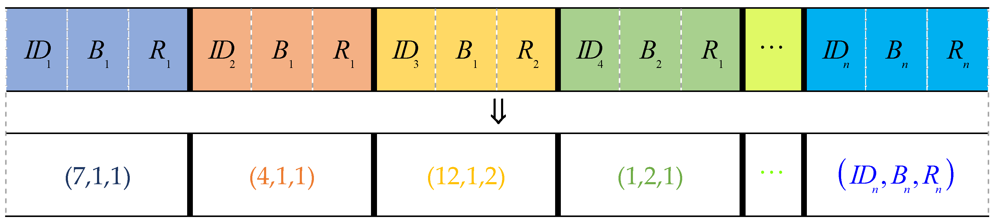A feasible solution is one in which a chromosome can be expressed, as shown in Figure 5.

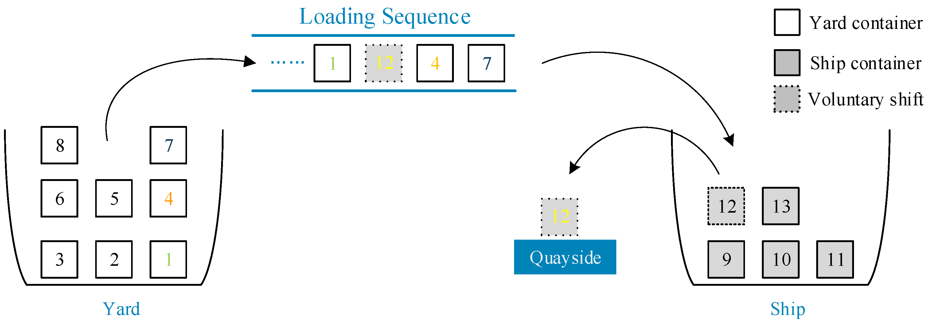
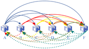
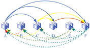
Figure 5 shows a legal chromosome code through which a complete loading plan can be obtained: L_p = 〈(7,1,1), (4,1,1), (12,1,2), (1,2,1), …〉. The first triplet (7,1,1) represents that container_7 was first loaded on the ship and its location on the ship was (bay1, row1), then container_4 was loaded onto the ship, and its position is (bay1, row1) as well. Container_12 is the “voluntary shift” container, i.e., the container on the ship. It needs to be temporarily moved to the side of the dock for container relocation at a future port, and then is loaded onto the ship according to the “new” loading sequence. Then, the container will be loaded in position (bay1, row2) after container_4 is loaded. A schematic diagram of the loading process is shown in Figure 6. The number in the figure represents the container number. The complete loading sequence is L_s = 〈7,4,12,1,…〉 and the loading sequence for the yard container is L^Y_s = 〈7,4,1,…〉 (L^Y_s ⊆ L_s). This information is found in the loading plan; L_p = 〈(7,1,1), (4,1,1), (12,1,2), (1,2,1), …〉 can be used to find the number of container shifts and the stowage plan, and the stability of the ship can then be calculated from the stowage plan. However, because container relocation is an NP-hard problem, the true value of the number of container shifts in the yard cannot be obtained in polynomial time when the loading plan L_p is given. Based on the literature [67], here we replace the optimal plan with a near-optimal plan based on a greedy heuristic. We have reason to adopt this approach, and it is in line with the actual production situation.

• Containers arrive at the terminal yard before they are loaded. The advance time is usually more than ten hours or a few days. Therefore, there is sufficient time for processing of the yard containers, such as pre-marshalling, to meet the requirements of loading containers in order of loading sequence. In addition, the cost of container shifts in a container yard is lower than shifts on ships.
• Different loading plans under the solution space many times must be verified and evaluated, and thus a fast and efficient heuristic is urgently needed.

4.3. Heuristic Rules for Relocation of Yard Containers

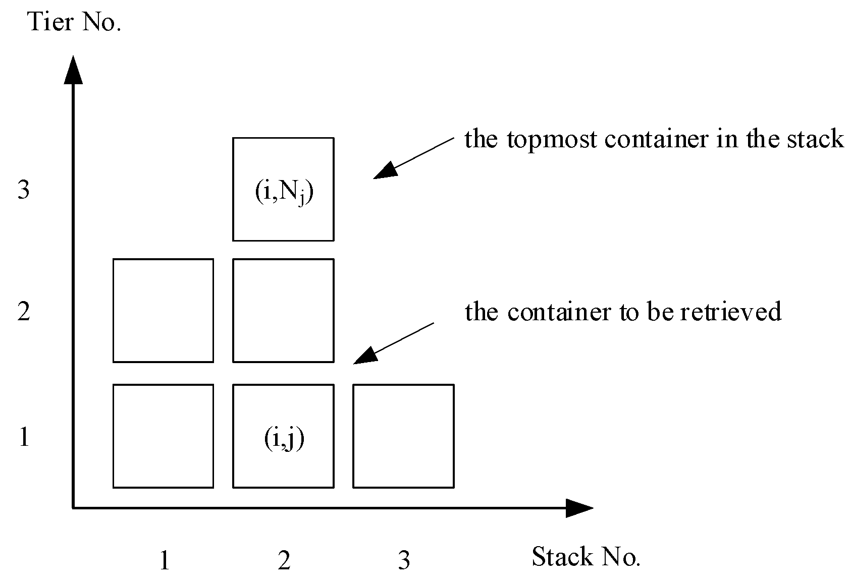
It is assumed that before the loading operation begins the storage status in the yard of the containers to be loaded and the loading sequence L^Y_s of the containers on the ship are both known. The shifting operation takes place in the same bay, and there are enough slots for relocation. Figure 7 shows a schematic diagram of a yard bay layout. We define (i, j) as the position corresponding to the row and tier in the container yard. R_i^N is defined as the total number of containers in stack i; thus, the total number in all bay stacks can be expressed as B^N = ${\displaystyle {\sum }_{i=1}^{r_Y}{R}_i^N}$. We define the priority, p_i,j, according to the order of the destination port of container (i, j); p_i,j = D represents the destination port of container (i, j) as D. The later the destination port, i.e., the larger the value of D, the earlier a container should be loaded on the ship. In other words, at the front end of the loading sequence the priority of a given container is higher. D_i^max is the maximum value of the destination port in the i-th stack and D_i^min is the minimum value of the destination port in the i-th stack, i.e., D_i^max = max{p_i,j | 1 ≤ j ≤ R_i^N} and D_i^min = min{p_i,j | 1 ≤ j ≤ R_i^N}.

The idea of a greedy heuristic algorithm is proposed in [67]. According to a given L^Y_s in the container loading sequence, a container (i, j) is the target container to be retrieved; the following operation strategy is then implemented until all containers are loaded on board.

• STRATEGY:
  • j = R_i^N: a container (i, j) is located at the top of the i-th stack and is retrieved directly.
  • j ≠ R_i^N: there is a blocking container (i, b) (b = j + 1, …R_i^N) when the container (i, j) is retrieved, and the blocking container needs to be temporarily relocated to stack k (k ≠ i). There may be only one blocking container, i.e., the top container (i, R_i^N) (b = R_i^N) in the i-th stack, or several, i.e., (b = j + 1, …R_i^N). According to the following rules, each blocking container is relocated to k (k ≠ i). The selection of stack k (k ≠ i) follows the following rules.
• RULE:
  • R_k^N < t_Y and p_i,b ≥ D_k^max: R_k^N < t_Y means that stack k has space to accommodate blocking containers, and relocation will not block the containers in stack k. If there are multiple stacks to choose from, choose the smallest D_k^max. If there is a tie, select the nearest one.
  • R_k^N < t_Y and p_i,b < D_k^max means that relocation will block the container in stack k. At this time, the smallest D_k^max should be selected. If there are multiple columns to choose from, choose the shortest column.

A feasible solution can be produced according to the above strategies and rules whenever there is a feasible solution.

4.4. Heuristic Rules for Container Voluntary Shifting

In Section 3.3 above, we defined voluntary shifts as shifts that occurs when to reorder the sequence of containers on the ship in order to prevent container relocation in the future. This is called the Myopic Voluntary Shifting Rule in [18,46], and the specific details of these heuristic rules can be found in these two works.

4.5. Generating Initial Population

Drawing lessons from the actual production experience of the container stowage plan, when generating the initial population P₀ of NSGA-III a two-stage method is used to generate the initial population of scale N.

Section 4.3 defines the priority, p_i,j, in the terminal yard. The farther away the destination port of container (i, j) is, the earlier the container will be loaded on the ship. At the same time, the larger the corresponding D (p_i,j = D) value, the higher the container’s priority. The concept of container priority is used in this section.

Stage 1: 

Randomly adopt the following two mechanisms to generate a loading sequence L_s for the feasible solution; pay attention to L_s = L^Y_s at this time.

1.

Retrieve the top container with the highest priority among all the columns of the yard containers each time, i.e., retrieve {C_Topmost | D_i^max, i ∈ all rows in the yard}. If there are more choices, choose the one with the highest quality.

2.

Retrieve the container with the highest priority in the current yard each time, i.e., retrieve {C_D_i^max, i ∈ all rows in the yard}. If there are more choices, choose the one with the fewest blocking containers. If there is a tie, retrieve the heaviest one.

Stage 2: 

In Stage 1, we obtain a complete loading sequence. Each container C in this given loading sequence must now be assigned to a specific ship stack. Due to the particular physical structure of container ships, their stacked containers follow the LIFO policy. Now, operating according to the following mechanism, we can finally obtain a feasible solution. In the above two stages, the strategy of voluntary shifts is not used. Therefore, there are no container shifts in the initial population.

1.

Suppose a stack k satisfies R_k^N < t_S and a container C does not block other containers in stack k, i.e., the priority of container C satisfies p_C ≤ D_k^min; then, select this stack. If there are multiple choices, choose the one with the smallest D_k^min value.

2.

If a stack with the properties mentioned above does not exist and container C blocks other containers in stack k, i.e., p_C > D_k^min, choose the one that satisfies R_k^N < t_S and has the largest D_k^min value in stack k.

4.6. Genetic Operations

Genetic manipulation is used to generate individual offspring, including by crossover and mutation. Crossover operates on a pair of chromosomes, while mutation operates only on a single individual.

First, consider one chromosome of only the yard containers CH_Y. Assuming that the chromosome contains only seven genes, that is, only seven yard containers (i.e., containers 1–7), set one parent chromosome as P1:〈(3,1,1), (2,2,1), (5,2,3), (1,1,2), (4,1,1), (7,2,2), (6,1,1)〉 and the other parent chromosome as P2:〈(4,2,1), (1,1,1), (6,1,2), (3,1,2), (5,2,2), (2,1,1), (7,1,1)〉. 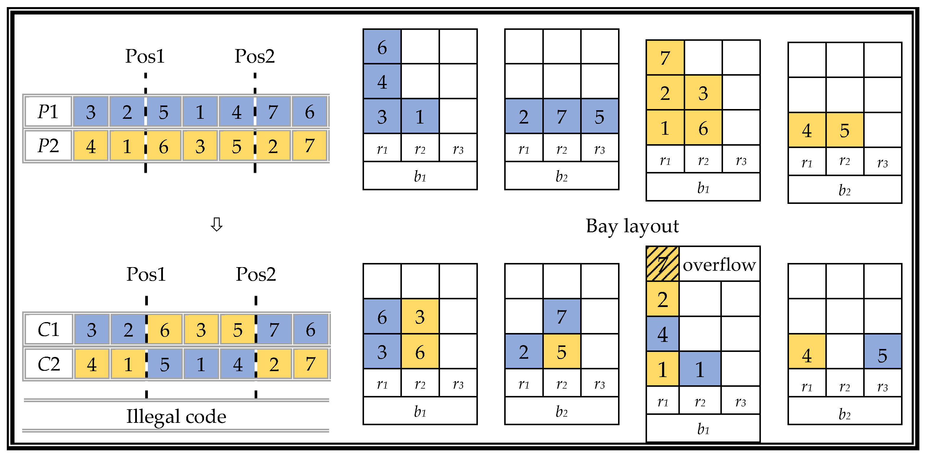In this example, the size of the container is set to b_S = 2, r_S = 3, t_S = 3. The crossover operation uses a double cut point crossover. In this example, the cut point positions are set to 2 and 5; the specific process of generating the two offspring chromosomes C1 and C2 is shown in Figure 8.

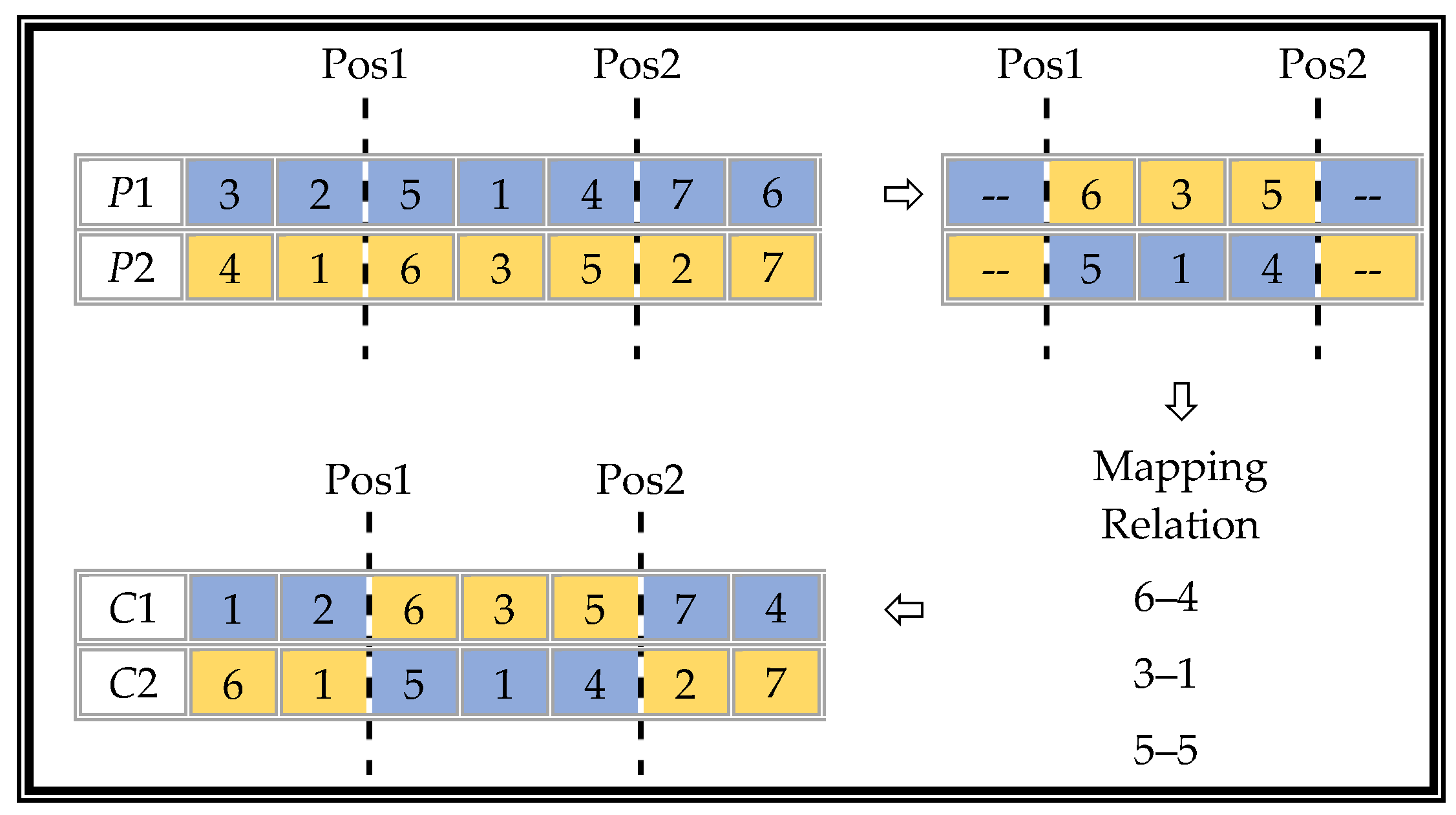
Two problems arise after the cross-recombination operation process. One is that the chromosome encoding of the offspring is illegal, and the other is that a certain row of containers exceeds its containment range, causing a stack overflow. In response to the above problems, we provide the following two renovations.

• RENOVATION:
  • A partially mapped crossover (PMX) uses a unique repair program to solve the illegality caused by a simple double-point intersection. The specific steps are shown in Figure 9.
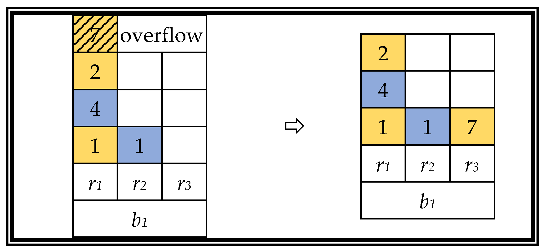
  • A greedy heuristic strategy is used to solve certain stack overflow problems, as follows. Load the container into the row with the least number of stacked containers in the same bay. If there are more choices, select the closest column. A schematic diagram of the stack overflow resolution strategy is shown in Figure 10.
    A complete loading plan includes both yard containers and ship containers that are voluntarily shifted. Consider the chromosome CH of both the yard container and the shipping container. This chromosome is added to five shipping containers (i.e., 8–12) based on the above CH_Y; thus, chromosome CH contains twelve genes. Due to voluntary shifts, the length of the chromosomes of the two parents will be different, i.e., the C_Y is the same and C_S (V) is not, which in turn leads to different positions of the cut points when addressing them. We provide a third repair strategy, called the addressing strategy, in response to this problem.

• RENOVATION:

  3.

  The addressing strategy is as follows. Mark the voluntary shifted containers in the loading sequence and record their relative positions. Ignore these containers; then, when determining the location of the tangent point, the chromosome gene will only contain the yard containers and will record the location of the tangent point at this time. The containers undergoing voluntary shifts can now be restored according to their previously-registered relative positions.

To obtain a complete chromosome, first determine the position of the tangent point of the double-point crossing according to the addressing strategy, then perform partial mapping and stack overflow repair, respectively, according to repair strategies 1 and 2 to obtain two legitimate offspring chromosomes.

After the crossover operation is performed, several offspring individuals in the population will be selected according to the mutation probability, P_m, to perform mutation operations in order to increase the diversity of the population and avoid falling into the local optimum. We have designed three types of operators to introduce a small amount of perturbation into the offspring genes and expand the search space to find more promising neighborhoods for exploration. A detailed introduction to specific operation operators is provided in Section 4.8.

4.7. Local Search

The local search we propose here is a kind of memetic algorithm that uses a selection mechanism similar to that in [68] to select certain individuals for local search. Local search is added to the framework of NSGA-III, that is, we introduce local search strategies into the iterative process of NSGA-III to realize the self-learning of individuals in the life cycle. After adding local search, NSGA-III uses local search to locally improve certain individuals, which can better balance the relationship between exploration and development in order to obtain a better solution with a higher probability.

First, we define the following aggregate function:

$$g\left(X|\lambda \right)={\lambda }_1\left(-f_{11}\left(X\right)\right)+{\lambda }_2\left|f_{12}\left(X\right)\right|+{\lambda }_3\left|f_{13}\left(X\right)\right|+{\lambda }_4{f}_{21}\left(X\right)+{\lambda }_5{f}_{22}\left(X\right)+{\lambda }_6{f}_{23}\left(X\right)$$

(11)

where λ = [λ₁,λ₂,…λ₆] is a weight vector, then the method of generating reference points in NSGA-III is used to generate a set of weight vectors that meet the constraints (as shown in Equation 12 and are uniformly distributed in the objective space. Therefore, the number of weight vectors is $C_{\zeta +5}^6$. If we set ζ in the equation to be 5, 252 weight vectors are generated for six-objective optimization problems.

$${\lambda }_1+{\lambda }_2+{\lambda }_3+{\lambda }_4+{\lambda }_5+{\lambda }_6=\zeta ,\begin{array}{c}\end{array}{\lambda }_i\in \left\{0,1,\cdots ,\zeta \right\},i=1,2,\cdots 6$$

(12)

When selecting an individual for local search, we first randomly choose one from these weight vectors using the aggregate function (12) as the comparison index and choose an elite solution through the tournament selection method without replacement. Then, a local search is performed on the solution to obtain one or a set of improved solutions. Algorithm 2 shows the local search process.

Algorithm2. Framework of local_search (Qt)

1: Q’t ← Ø

2: for i = 1 to $\lfloor N\times P_{ls}\rfloor$ do

3: The weight vector λ is randomly selected from the set of weight vectors

4: S ← Tournament Selection with Replacement (Q’t, λ)

5: Ei ← Local Search for Individual (S, λ, l_ier)

6: Q’t ← Q’t ∪Ei

7: end for

8: return Q’t

Here, $\lfloor N\times P_{ls}\rfloor$ represents the number of offspring populations selected to perform a local search and/is the probability of a local search. In other words, the selection operation of “select the elite solution and apply the local search” is repeated/times. As is well-known, local search requires a great deal of calculation time; thus, only a portion of offspring individuals can be selected for local search. If a partial improvement is made to an individual offspring, three types of neighborhood operations that are similar to mutation operations are randomly selected and applied to each selected offspring. This operation is performed l_ier times.

4.8. Neighborhood Operator

There is one last key issue in the algorithm that needs to be explained, namely, the neighborhood operator applied to the mutation operator and how to search locally. In the variant of NSGA-III presented here, the proposed neighborhood calculation is directed at the loading plan, L_p, rather than the solution S, which helps to introduce knowledge related to the optimization problem of container stowage. Therefore, each generated neighborhood must be calculated.

In Section 4.2., we defined a complete loading plan as consisting of a loading sequence L_s and the specific location group of a given container on the ship, i.e., L_p = 〈(ID₁, B₁, R₁), (ID₂, B₂, R₂), …, (ID_n, B_n, R_n)〉. According to the scope and effect of the neighborhood operator, the neighborhood operator is divided into the following three categories.

1.

Operators applied to the loading sequenceL_s: this type only acts on the loading sequence, including three operators.

(1)

Forward shift operator: two indexes x and y (1 ≤ x < y ≤ n) are randomly generated, then the triplet (ID_y,B_y,R_y) is shifted forward to the position of x−1. At this time, the loading plan is L_p = 〈(ID₁,B₁,R₁), …, (ID_y,B_y,R_y), (ID_x,B_x,R_x),…, (ID_n,B_n,R_n)〉.

(2)

Backward shift operator: two indexes x and y (1 ≤ x < y ≤ n) are randomly generated, then the triplet (ID_x,B_x,R_x) is shifted back to the position of y + 1. At this time, the loading plan is L_p = 〈(ID₁,B₁,R₁), …, (ID_y,B_y,R_y), (ID_x,B_x,R_x),…, (ID_n,B_n,R_n)〉.

(3)

ID_swap operator: two indexes x and y (x ≠ y) are randomly generated, then the sequential positions of the two triplets of (ID_x, B_x, R_x) and (ID_y, B_y, R_y) are swapped.

The loading plan obtained after applying this type of operation operator remains feasible.

2.

Operators applied to the stack of the container ship: this operator will change the container stack information in the loading plan, mainly including the following two operators.

(1)

Reassign operator: one index x (1 ≤ x ≤ n) and a container ship slot A are randomly generated; slot A satisfies t_A ≤ t_S and is not in the same position as a slot (B_x, R_x) corresponding to (ID_x, B_x, R_x), i.e., (B_A, R_A) ≠ (B_x, R_x). Then, replace (ID_x, B_x, R_x) with (ID_x, B_A, R_A) in the former loading plan L_p to obtain a new neighbor loading plan.

(2)

Container slot swap operator: two indexes x and y (1 ≤ x < y ≤ n) are randomly generated, then their slot position information is exchanged. At this time, the loading plan is L_p = 〈(ID₁,B₁,R₁), …, (ID_x,B_y,R_y),…, (ID_y,B_x,R_x) …, (ID_n,B_n,R_n)〉.

3.

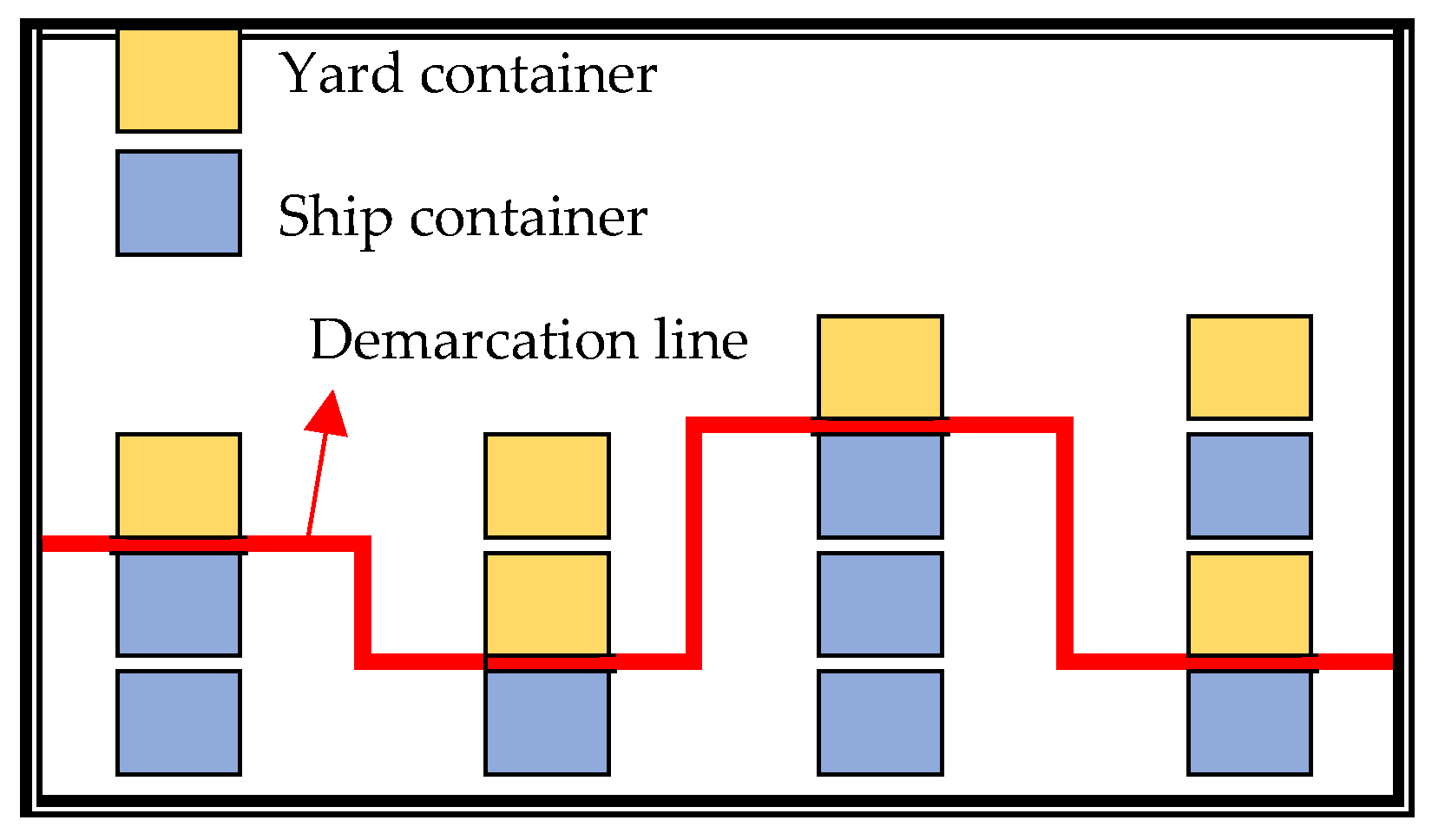
Operators applied to voluntary shifts: As mentioned earlier, in order to reduce the number of container shifts in future ports certain containers C_S (V) will be temporarily placed on the quay shore and on the containers in the yard before being loaded back onto the ship. Two operators are proposed to add or reduce containers for the set C_S (V).

To better explain the following operating procedures, we first define the concept of the “demarcation line”. The “demarcation line” is a vertical partition that divides the final ship container layout into two parts. The upper part of the demarcation line consists of the yard container C_Y and the voluntary shift container C_S (V), i.e., C_Y ∪ C_S (V); the lower part is the container on the ship, i.e., C_S\C_S (V), except for the part undergoing the voluntary shift. Figure 11 shows an example of the “demarcation line”.

(1)

To add a voluntary relocation container, randomly select a container below the demarcation line and activate it as a voluntary shift container, ID_s. The original position of the selected container should have two or more containers in the stack, and it should be at the uppermost position f of the lower part of the demarcation line. Then, randomly insert the container into the loading plan and randomly assign a position to it to obtain a neighborhood loading plan, i.e., 〈(ID₁,B₁,R₁), …, (ID_i-1,B_i-1,R_i-1), (ID_s,B_s,R_s), (ID_i,B_i,R_i)…, (ID_n,B_n,R_n)〉.

(2)

To remove a voluntary relocation container, randomly select a voluntary relocation container in the upper part of the dividing line and remove it from the loading plan.

5. Experiment and Analysis

In this section, we describe a series of numerical experiments used to test the effectiveness of the algorithm proposed in this paper and the design a comparative experiment involving other optimization methods. The experimental results are analyzed and discussed in the following sections. The test data are explained in Section 5.1; a comprehensive evaluation index of the experimental results is provided in Section 5.2; the parameter settings used in the experiment and the comparison experiment with other algorithms are provided in Section 5.3; and Section 5.4 lists the results of the test and the analysis of the results. The algorithm proposed in this paper was implemented in MATLAB R2019b (win64). All experiments were performed on a Windows server with 16.0 GB RAM and an Intel (R) Core (TM) i7 processor clocked at 3.0 GHz. The times used in the text are the CPU seconds of this machine.

5.1. Setting Data

To verify the effectiveness and practicability of our proposed algorithm, we set up 48 sets of calculation examples for the experiment according to the ship structure and stacking methods. The examples are summarized in

Table 3. Experimental example.

Instance		YARD				SHIP
		bY	rY	tY	NY	bS	rS	tS	NS
1A	1B	2	4	5	21	4	4	5	20
2A	2B	4	4	5	46	8	4	5	33
3A	3B	2	4	8	36	4	4	8	38
4A	4B	4	4	8	79	8	4	8	66
5A	5B	2	8	5	46	4	8	5	41
6A	6B	4	8	5	109	8	8	5	73
7A	7B	2	8	8	70	4	8	8	73
8A	8B	4	8	8	182	8	8	8	130
9A	9B	2	4	5	23	4	4	5	24
10A	10B	4	4	5	41	8	4	5	34
11A	11B	2	4	8	35	4	4	8	29
12A	12B	4	4	8	101	8	4	8	60
13A	13B	2	8	5	60	4	8	5	47
14A	14B	4	8	5	99	8	8	5	65
15A	15B	2	8	8	75	4	8	8	69
16A	16B	4	8	8	188	8	8	8	130
17A	17B	2	4	5	28	4	4	5	16
18A	18B	4	4	5	40	8	4	5	48
19A	19B	2	4	8	46	4	4	8	37
20A	20B	4	4	8	100	8	4	8	69
21A	21B	2	8	5	56	4	8	5	41
22A	22B	4	8	5	97	8	8	5	75
23A	23B	2	8	8	65	4	8	8	62
24A	24B	4	8	8	168	8	8	8	103

. All containers are 20 ft in size, the weight in group A is set to unit 1, and the weight of containers in group B ranges from unit 10 to unit 20. b_Y, r_Y, t_Y, and N_Y represent the number of bays, the number of stacks, the height of the layer, and the number of yard containers, respectively, in each group of calculation examples. Similar to the yard containers, the relevant values concerning the ship are set to b_S, r_S, t_S, and N_S. The value set indicates the different bay position structures, which ensures enough places to accommodate the containers.

A rectangular structure is adopted for the ship or yard bay structure and different layers and numbers of columns are set. Each type of bay structure has a different bay layout randomly generated according to certain principles. The principle of generating the bay position layout is as follows: the containers in the yard bay are 50~80% of the total amount of the bay capacity and the shipping container occupancy rate is 20~30%; according to different destinations, different priorities are generated according to which more distant destinations have higher priority. We set six different priorities in this article.

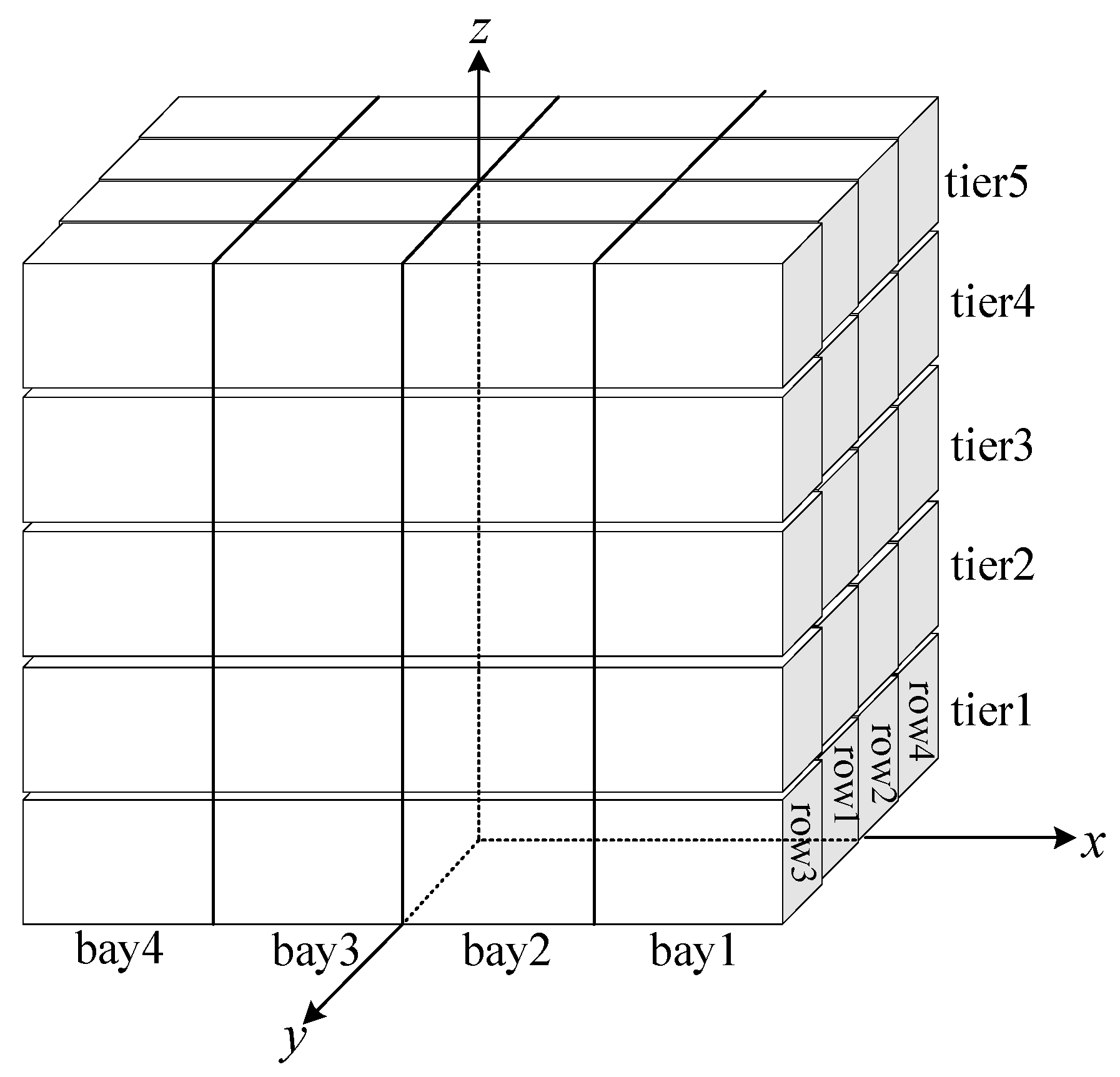
The establishment of the ship coordinate system is intended to accurately express the spatial position of any point on the ship, which is convenient for positional determinations and ship performance calculations. According to our assumptions the ship is considered as a box structure, and we use the O-xyz rectangular coordinate system fixed on the ship, as shown in Figure 12.

Assuming that the center of gravity of the container is at the geometric center, this is true in practice as well. As the container is a cube with a side length of 1, the coordinates of the center of gravity of each container can be obtained according to the coordinate system we have established. The ship in the example consists of four bays (bay1~bay4), each bay has four stacks (row1~row4), and each stack has five layers (tier1~tier5); thus, the coordinates of the center of gravity of each container in this example are as shown in

Table 4. Container ship slot location index.

$\mathbf{Slot}\mathbf{No}.({\mathit{b}}_{\mathit{S}},{\mathit{r}}_{\mathit{S}},{\mathit{t}}_{\mathit{S}})$	$\mathbf{Center}\mathbf{of}\mathbf{Gravity}(\mathit{x},\mathit{y},\mathit{z})$
(1, 1, 1)	(1.5, 0.5, 0.5)
(1, 2, 1)	(1.5, −0.5, 0.5)
(1, 3, 1)	(1.5, 1.0, 0.5)
$⋮$	$⋮$
(4, 4, 5)	(−1.5, −1.5, 4.5)

.

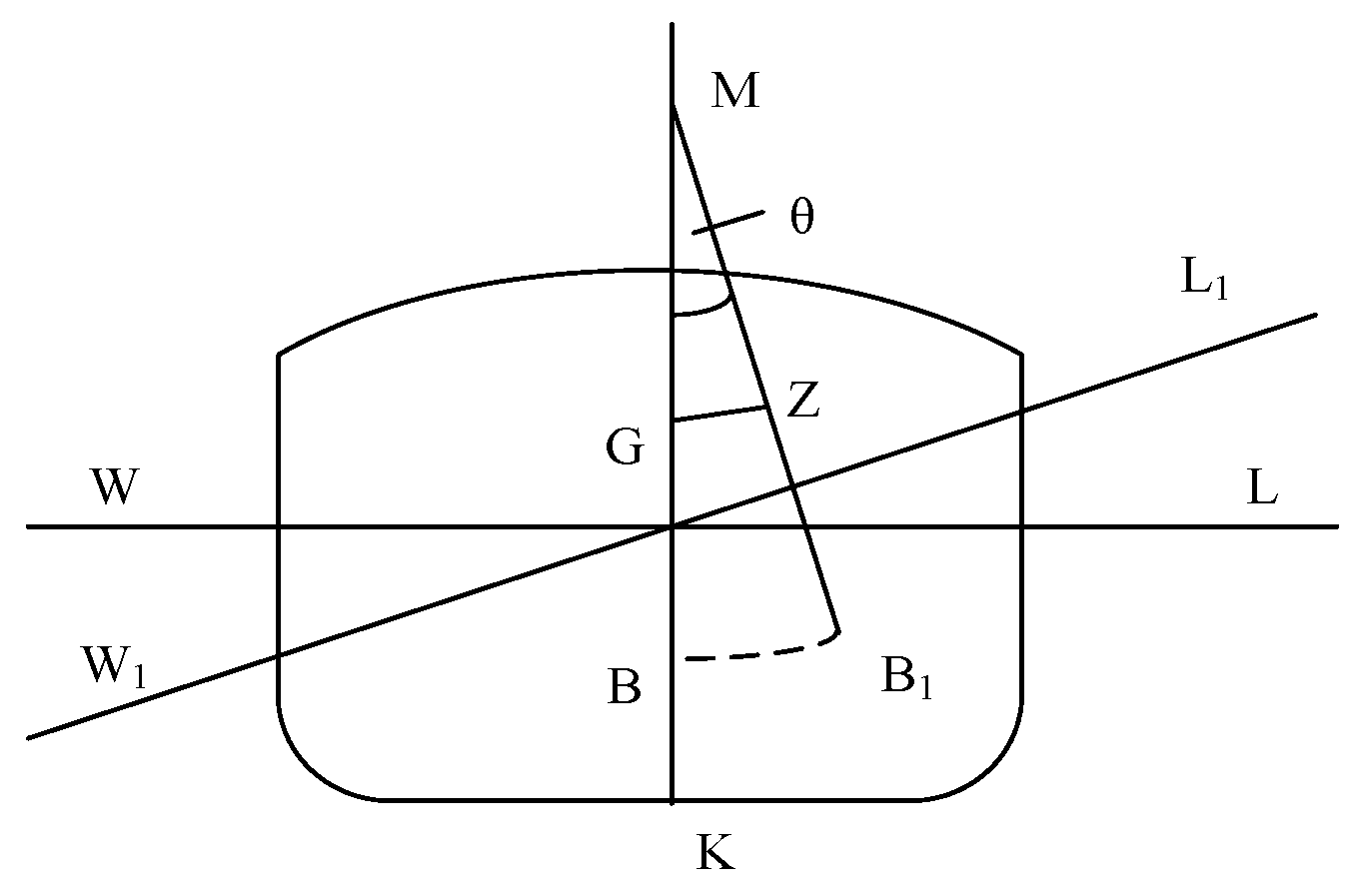
The essence of the stability calculation for different loading plans (i.e., different solutions) is the problem of “variation of weight in the ship”, which conforms to the attributes of the ship displacement and metacenter position (i.e., KM) invariants. According to the above settings, the three objective functions in the category of ship stability (i.e., the ship’s initial transverse metacentric height, heel angle, and trim) can be expressed as (1) $f_{11}=\min \left\{\frac{{\displaystyle \sum p_i{z}_i}}{{\displaystyle \sum p_i}}|i\in C_Y\cup C_S\left(V\right)\right\}$; (2) $f_{12}=\min \left\{\frac{\left|{\displaystyle \sum p_i{y}_i}\right|}{{\displaystyle \sum p_i}}|i\in C_Y\cup C_S\left(V\right)\right\}$; (3) $f_{13}=\min \left\{\frac{\left|{\displaystyle \sum p_i{x}_i}\right|}{{\displaystyle \sum p_i}}|i\in C_Y\cup C_S\left(V\right)\right\}$ where ${\rho }_i$ represents the weight of the i-container.

5.2. Performance Indicators

Researchers have proposed many methods for evaluating the performance of objective evolutionary algorithms, which can be summarized into three categories. The first type is used to assess the tightness between the computed set and the true Pareto-optimal surface, and is mainly used to evaluate the convergence of the algorithm. Here, we use the index of coverage between two solution sets (CS). The second category is used to assess the distribution of the solution set; here we use the maximum spread (MS). The third category allows for comprehensive consideration of the convergence and distribution of the solution set in order to evaluate the comprehensive performance of the solution. Here, we use the inverse generation distance (IGD).

In 2000, Zitzler proposed an evaluation method to compare the relative coverage of the two solution sets in the algorithm [69]. Assuming that P′ ⊆ P and P″ ⊆ P are two solution sets in the objective space (with P being the objective space solution set) and the coverage ratio is between P′ and P″ (two set coverage, CS), the equation is as follows:

$$CS\left(P^{\prime },P^{″}\right)\triangleq \frac{\left|\left\{a^{″}\in P^{″}|\exists a^{\prime }\in P^{\prime },a^{″}\succcurlyeq a^{″}\right\}\right|}{\left|P^{″}\right|}$$

(13)

If all points in P′ dominate or are equal to all points in P″, then CS = 1 can be defined; otherwise, CS = 0. Suppose CS (P′, P″) > CS (P″, P′); in that case, the dominance relationship of P′ is considered to be better than that of P″. Generally speaking, the intersection of the two solution sets P′ and P″ is not empty CS (P′, P″), and therefore CS (P″, P′) must be considered together when evaluating an algorithm.

The Maximum Spread (MS) evaluation method (known as the D method) is used to measure the spreading performance of the solution set distribution of the algorithm. The larger the MS value, the better the extension performance of a solution set. In particular, when the MS is 1, the solution set completely covers the entire real Pareto front. Assuming that P′⊆ P is a non-dominated solution set in the objective space, the for the MS value is calculated as follows:

$$MS\left(P^{\prime }\right)=\sqrt{{\displaystyle \sum _{i=1}^M{\left(\underset{a^{\prime }\in P^{\prime }}{\max }\frac{f_i\left(a^{\prime }\right)-f_i^{\min }}{f_i^{\max }-f_i^{\min }}-\underset{a^{\prime }\in P^{\prime }}{\min }\frac{f_i\left(a^{\prime }\right)-f_i^{\min }}{f_i^{\max }-f_i^{\min }}\right)}^2}}$$

(14)

where f_i^min and f_i^max represent the minimum and maximum values of the i-th goal (total M) in the objective space solution.

Inverted Generational Distance (IDG) is the inverse mapping of Generational Distance. It uses the average distance from the individual in the Pareto-optimal solution set, P*, to the non-dominated solution set P′ obtained by the algorithm. Therefore, it is calculated as follows:

$$IGD(P^{\prime },P*)=\frac{1}{\left|P*\right|}{\displaystyle \sum _{a^{\prime }\in P^{\prime }}\underset{a*\in P*}{\min }}\begin{array}{c}d\left(a^{\prime },a*\right)\end{array}$$

(15)

where d (a’, a*) represents the Euclidean distance between solutions a’ and a* in the objective space solution. The calculation expression is as follows:

$$\begin{array}{cc}d\left(a^{\prime },a*\right)& =\sqrt{{\displaystyle \sum _i^M{\left(\frac{f_i\left(a^{\prime }\right)-f_i^{\min }}{f_i^{\max }-f_i^{\min }}-\frac{f_i\left(a*\right)-f_i^{\min }}{f_i^{\max }-f_i^{\min }}\right)}^2}}\\ & =\sqrt{{\displaystyle \sum _i^M{\left(\frac{f_i\left(a^{\prime }\right)-f_i\left(a*\right)}{f_i^{\max }-f_i^{\min }}\right)}^2}}\end{array}$$

(16)

If |P*| can represent the Pareto front fully, then IGD (P′, P*) can, in a certain sense, comprehensively measure the convergence and diversity of the solution set. Because the solution set P′ must be close enough to the Pareto front surface in the objective space in order to obtain a smaller value of IGD (P′, P*), that is, the smaller the value of IGD, the better, and any part of P* has a corresponding solution to represent in P′, in an ideal situation solving the algorithm is a process of continuously approaching the optimal boundary P* and finally reaching the optimal boundary. However, in practical applications it is often difficult to find the true Pareto optimal surface. Here, P* is the Pareto front of all solutions obtained in all comparison algorithms in our experiment.

5.3. Parameter Setting and Comparison Algorithm

The parameter settings of the numerical calculation are shown in

Table 5. Parameter setting for algorithms.

Parameters	Value	Foundation
Population size N	100	Rule of thumb
Reference point number H	126	Equivalent to population size
Crossover probability Pc	100%	Experimentally obtained
Mutation probability Pm	5%	Experimentally obtained
Local search probability Pls	20%	Experimentally obtained
Local search iterations ls_ier	100	Rule of thumb
Tournament size τ	10	Rule of thumb
Termination principle	Limit time is 3 min	Experimentally obtained

. Because the result of the calculation provides a set of Pareto optimal solutions, allowing the decision-maker to compromise the choice, we therefore set the population size to 100 based on experience. The algorithm uses the systematic method proposed by Das and Dennis to generate structured reference points. The number of reference points generated by this method depends on the number of objective functions M and another positive integer p, where p represents the goal of evenly dividing each dimension into p parts; the equation is $H=C_{p+M-1}^{M-1}$ [70]. According to [64], the number of reference points should be equivalent to the population size. Therefore, we set the value of p to be equal to 4 and the number of reference points to 126.

We used calculation examples 1A and 1B to find the optimal P_c and P_m by adjusting different crossover probabilities and recombination probabilities while keeping the other parameters unchanged. For each set of calculation examples, we performed 30 independent calculations and used average result as the final output value. P* is the set of non-dominated solutions for all operations. The average IGD of 30 operations is provided in

Table 6. Parameter optimization of crossover probability and mutation probability.

	Pm	0	5	10	20
Pc
0		0.0276	0.0273	0.0308	0.0503
50		0.0249	0.0230	0.0296	0.0479
80		0.0207	0.0189	0.0307	0.0512
100		0.0198	0.0106	0.0284	0.0551

, and the best result (i.e., the smallest value 0.0106) is marked in bold. It can be seen from Table 6 that the crossover probability, P_c, has a more significant impact on the comprehensive performance of the algorithm. Therefore, we set the crossover probability to 100% and the mutation probability to 5%.

As described in Section 4.8, we designed three kinds of neighborhood operators for local search and mutation. To verify the influence of neighborhood operators on the algorithm’s performance, we set up comparative experiments. The results of this comparative experiment are shown in

Table 7. The influence of different neighborhood operators on the NSGA-III.

N1	N2	N3	N1 + N2	N1 + N3	N2 + N3	N1 + N2 + N3
0.0348	0.0305	0.0328	0.0279	0.0273	0.0246	0.0209

. The comprehensive version of the algorithm under each combination (i.e., average IGD) is provided as well.

From Table 7, it can be seen that the operator acting on the container stack (i.e., N2) has the most significant impact on the algorithm, the operator working on the loading sequence (i.e., N1) has the second-most, and the operator (i.e., N3) acting on the voluntary shifts has the least impact on the algorithm. When all operation operators are included, the algorithm’s overall performance is the best; thus, the neighborhood operator we proposed has a positive impact on the algorithm’s performance.

In our experiment, we designed six different algorithms; the related explanations of these algorithms are provided in

Table 8. Algorithms used in the comparative experiment.

Abbreviation	Algorithm	Decision-Making Methods	Parameter Setting
NSGA-III-L	NSGA-III with local search	Posterior	Same as Table 5.
NSGA-III-NL	NSGA-III without local search	Posterior	Same as Table 5, but it does not include local search parameters.
NSGA-II-L	NSGA-III with local search	Posterior	Same as Table 5, but it does not include reference point parameters.
NSGA-II-NL	NSGA-II without local search	Posterior	Same as Table 5, but it does not include reference points and local search parameters.
RWGA-L	RWGA with local search	Prior	Same as Table 5, but it does not include reference point parameters.
RWGA-NL	RWGA without local search	Prior	Same as Table 5, but it does not include reference points and local search parameters.

. As previously mentioned, in order to comprehensively evaluate the performance of the proposed algorithm it is necessary to obtain the true Pareto front. However, due to the complexity of the MaO-CSPP, the true Pareto front cannot be obtained in polynomial time. Therefore, the best possible approximate solution must be found. We compared the other five algorithms to obtain the best approximate solution P*. In Table 8, RWGA is a random weighted genetic algorithm, a better algorithm in the priori technology. Specific details regarding the algorithm can be found in [54].

5.4. Results and Discussion

According to the parameter settings in Section 5.3, we conducted experiments on each algorithm. Each algorithm was applied to the 48 instances generated in Section 5.1, and each instance of examples of each algorithm was independently run 30 times. Then, according to the performance indicators set in Section 5.2, the average value of each instance indicator was obtained. The average values of the indicators are summarized in

Table 9. Experimental results of IGD.

Instance	NSGA-III-L	NSGA-III-NL	NSGA-II-L	NSGA-II-NL	RWGA-L	RWGA-NL
1A	0.0287	0.0170	0.0531	0.0666	0.1074	0.1293
2A	0.0158	0.0534	0.0422	0.0502	0.1413	0.1341
3A	0.0998	0.0592	0.1259	0.1394	0.2465	0.2827
4A	0.1071	0.1044	0.1329	0.1417	0.2478	0.3082
5A	0.0467	0.0520	0.0752	0.1215	0.1783	0.1895
6A	0.0630	0.0615	0.1119	0.1608	0.1842	0.2643
7A	0.0856	0.0576	0.1152	0.1830	0.1955	0.2368
8A	0.0810	0.0729	0.1017	0.1601	0.2049	0.2588
9A	0.0606	0.0868	0.0749	0.1214	0.1582	0.1736
10A	0.0579	0.0733	0.0866	0.1284	0.2471	0.2711
11A	0.1051	0.1222	0.1494	0.2009	0.2566	0.3077
12A	0.1067	0.1352	0.1771	0.1699	0.2433	0.2941
13A	0.0349	0.0626	0.1529	0.2138	0.2489	0.3691
14A	0.0725	0.0851	0.1414	0.1891	0.2595	0.3060
15A	0.1508	0.1098	0.2546	0.3136	0.3712	0.4004
16A	0.1688	0.1450	0.2516	0.3070	0.3362	0.3910
17A	0.0899	0.0997	0.1463	0.2094	0.2687	0.3085
18A	0.0952	0.1300	0.1919	0.2310	0.2635	0.3261
19A	0.1190	0.1254	0.2116	0.2701	0.3103	0.3718
20A	0.1407	0.1640	0.2691	0.3409	0.3770	0.4419
21A	0.0716	0.0683	0.1653	0.2093	0.2522	0.3165
22A	0.0607	0.0651	0.2002	0.2393	0.3031	0.3453
23A	0.0935	0.0640	0.1487	0.1897	0.2366	0.3165
24A	0.1015	0.0784	0.1890	0.2228	0.2698	0.3886
Average	0.0857	0.0872	0.1487	0.1908	0.2462	0.2972
1B	0.0306	0.0195	0.0503	0.0576	0.2452	0.2858
2B	0.0092	0.0122	0.0535	0.0666	0.1777	0.2320
3B	0.1565	0.1658	0.2242	0.2829	0.3731	0.4177
4B	0.1078	0.1171	0.1887	0.2484	0.3057	0.3390
5B	0.0414	0.0329	0.1071	0.1460	0.2585	0.3535
6B	0.0720	0.0647	0.1069	0.1700	0.2555	0.3285
7B	0.0809	0.0916	0.1313	0.1443	0.2718	0.3618
8B	0.0968	0.1072	0.1561	0.2092	0.3119	0.4070
9B	0.0546	0.0461	0.1129	0.1673	0.2780	0.3665
10B	0.0846	0.0842	0.1398	0.1795	0.2720	0.3322
11B	0.1067	0.0889	0.1690	0.2134	0.3179	0.4394
12B	0.1195	0.1112	0.1797	0.2138	0.3514	0.4213
13B	0.0612	0.0814	0.1808	0.2499	0.3708	0.4430
14B	0.0640	0.0768	0.2162	0.2590	0.3682	0.4277
15B	0.1697	0.1866	0.2368	0.2912	0.3667	0.4250
16B	0.1536	0.1751	0.2289	0.2879	0.3820	0.4315
17B	0.0990	0.1160	0.1893	0.2372	0.3208	0.4764
18B	0.1096	0.1292	0.1978	0.2361	0.3549	0.4847
19B	0.1720	0.1922	0.2684	0.3154	0.4065	0.5108
20B	0.1483	0.1734	0.1802	0.2200	0.3278	0.4397
21B	0.0999	0.1119	0.1511	0.2110	0.2510	0.3519
22B	0.0872	0.1102	0.1898	0.2375	0.2952	0.3921
23B	0.1397	0.1646	0.1845	0.2312	0.2726	0.3772
24B	0.1482	0.1851	0.2165	0.2540	0.3053	0.4671
Average	0.1005	0.1102	0.1692	0.2137	0.3100	0.3963

,

Table 10. Experimental results of CS.

Instance	NSGA-III-L/NSGA-II-L		NSGA-III-L/RWGA-L		NSGA-II-L/RWGA-L
	$\mathit{C}\mathit{S}\left({\mathit{P}}^{\prime },{\mathit{P}}^{″}\right)$	$\mathit{C}\mathit{S}\left({\mathit{P}}^{″},{\mathit{P}}^{\prime }\right)$	$\mathit{C}\mathit{S}\left({\mathit{P}}^{\prime },{\mathit{P}}^{″}\right)$	$\mathit{C}\mathit{S}\left({\mathit{P}}^{″},{\mathit{P}}^{\prime }\right)$	$\mathit{C}\mathit{S}\left({\mathit{P}}^{\prime },{\mathit{P}}^{″}\right)$	$\mathit{C}\mathit{S}\left({\mathit{P}}^{″},{\mathit{P}}^{\prime }\right)$
1A	0.0055	0.0086	0.2024	0.0168	0.0129	0.3528
2A	0.1184	0.0806	0.1953	0.0106	0.0053	0.6876
3A	0.8457	0.0014	0.5421	0.0353	0.3693	0.1820
4A	0.7454	0.0009	0.3636	0.0351	0.1898	0.3810
5A	0.4447	0.0005	0.3398	0.0855	0.1706	0.0114
6A	0.4410	0.0002	0.1971	0.2970	0.1814	0.0162
7A	0.9285	0.0000	0.2961	0.0243	0.0066	0.7916
8A	0.9354	0.0002	0.3037	0.0054	0.0081	0.5881
9A	0.9453	0.0004	0.2513	0.0161	0.0080	0.6791
10A	0.9557	0.0006	0.4725	0.0148	0.0012	0.5036
11A	0.9510	0.0007	0.3775	0.0063	0.0040	0.4112
12A	0.9547	0.0003	0.4662	0.0336	0.0221	0.4146
13A	0.9008	0.0007	0.3022	0.0125	0.0132	0.7542
14A	0.8950	0.0016	0.3401	0.0239	0.1297	0.0307
15A	0.9187	0.0015	0.3597	0.0202	0.0030	0.4894
16A	0.9369	0.0010	0.3912	0.0405	0.0087	0.4266
17A	0.9703	0.0002	0.2515	0.3400	0.0025	0.9035
18A	0.9516	0.0010	0.1415	0.2504	0.0037	0.8372
19A	0.9115	0.0004	0.2013	0.0215	0.0022	0.6931
20A	0.9328	0.0011	0.1506	0.0091	0.0019	0.5981
21A	0.9289	0.0004	0.3145	0.0205	0.0057	0.3948
22A	0.9175	0.0021	0.3217	0.0063	0.0019	0.7926
23A	0.9143	0.0018	0.4593	0.0459	0.0012	0.4867
24A	0.9379	0.0011	0.2452	0.0203	0.0118	0.5894
Average	0.8078	0.0045	0.3119	0.0580	0.0485	0.5006
1B	0.9315	0.0009	0.0203	0.1635	0.0010	0.4136
2B	0.9067	0.0012	0.0949	0.0089	0.0014	0.7476
3B	0.8207	0.0011	0.8871	0.0142	0.0000	0.3765
4B	0.7234	0.0006	0.6692	0.2117	0.0011	0.4380
5B	0.6217	0.0005	0.5345	0.0176	0.0009	0.9457
6B	0.7543	0.0002	0.1546	0.2471	0.0001	0.4231
7B	0.8840	0.0000	0.1927	0.2851	0.0005	0.7905
8B	0.9610	0.0003	0.1997	0.0116	0.0006	0.5886
9B	0.9445	0.0004	0.2063	0.0020	0.0000	0.7278
10B	0.9755	0.0004	0.0452	0.1909	0.0000	0.5441
11B	0.9529	0.0005	0.1816	0.0867	0.0003	0.4537
12B	0.9474	0.0004	0.1726	0.0208	0.0000	0.5152
13B	0.9038	0.0006	0.1998	0.3011	0.0000	0.7571
14B	0.9344	0.0009	0.0733	0.1682	0.0000	0.6884
15B	0.9123	0.0012	0.0290	0.1271	0.0020	0.4891
16B	0.9405	0.0007	0.0297	0.1298	0.0001	0.4713
17B	0.9709	0.0002	0.0253	0.1239	0.0008	0.9040
18B	0.9614	0.0004	0.2094	0.0145	0.0005	0.8446
19B	0.9045	0.0004	0.1648	0.0114	0.0000	0.6908
20B	0.9573	0.0005	0.1735	0.0117	0.0000	0.6064
21B	0.9268	0.0005	0.2704	0.0254	0.0004	0.4498
22B	0.9337	0.0012	0.2041	0.0061	0.0002	0.8011
23B	0.9484	0.0012	0.2698	0.0185	0.0000	0.5480
24B	0.9781	0.0007	0.0241	0.1645	0.0000	0.6497
Average	0.9040	0.0006	0.2097	0.0984	0.0004	0.6194

and

Table 11. Experimental results of MS.

Instance	NSGA-III-L	NSGA-III-NL	NSGA-II-L	NSGA-II-NL	RWGA-L	RWGA-NL
1A	0.5408	0.5238	0.9984	1.0123	0.7480	0.7299
2A	0.4742	0.4226	0.7818	1.0621	0.8436	0.7917
3A	0.8573	0.9051	1.0156	1.2058	0.3746	0.3264
4A	0.9093	0.9513	1.0573	1.2056	0.4412	0.3902
5A	0.7898	0.8895	1.0662	1.1014	0.2685	0.2143
6A	0.6890	0.8275	0.9759	0.5785	0.4288	0.3746
7A	0.8951	0.8490	1.0505	0.7112	0.3989	0.3486
8A	0.8991	0.8536	1.0206	0.6997	0.2850	0.2444
9A	0.9310	0.9493	1.0973	1.1554	0.2237	0.1794
10A	0.9503	1.0157	1.1194	1.1509	0.2475	0.2493
11A	0.9936	1.0590	1.1480	1.2002	0.6978	0.6164
12A	0.9645	0.9926	1.1490	1.2914	0.3995	0.3419
13A	0.8530	0.8943	1.1382	1.3826	0.1348	0.1251
14A	0.8760	0.9053	1.1299	1.3278	0.1299	0.1208
15A	1.1138	1.0450	1.1086	1.3941	0.3323	0.2949
16A	1.0403	1.0832	1.1671	1.4472	0.4738	0.4126
17A	0.9007	0.9573	1.1777	1.5991	0.5096	0.4484
18A	0.8911	0.9646	1.1471	1.6920	0.5116	0.4607
19A	0.9476	0.9992	1.1509	1.5409	0.3640	0.3161
20A	0.8489	0.9080	1.1211	1.3402	0.3709	0.3145
21A	1.1569	1.2078	1.2953	1.6115	0.5024	0.4486
22A	1.0683	1.2139	1.3144	1.6829	0.3636	0.3153
23A	1.4845	1.5418	1.5842	1.9961	0.1732	0.1245
24A	1.1072	1.1343	1.2337	1.6254	0.3596	0.2968
Average	0.9243	0.9622	1.1270	1.2923	0.3993	0.3536
1B	0.6005	0.5568	1.0564	1.2016	0.6780	0.6481
2B	0.5297	0.5425	1.0733	1.1803	0.7900	0.7923
3B	0.9067	0.8225	1.0046	1.1376	0.3072	0.2252
4B	0.9674	0.9101	1.1196	1.3278	0.3920	0.3405
5B	0.8888	0.8320	1.1515	1.3434	0.2358	0.1614
6B	0.7847	0.8949	1.1422	1.3895	0.3778	0.3305
7B	0.9839	1.0291	1.1514	1.3808	0.3664	0.3028
8B	1.0717	1.0962	1.1500	1.4220	0.2286	0.1704
9B	1.0331	1.0844	1.0845	1.1981	0.1747	0.1229
10B	1.0376	1.0788	1.1274	1.2048	0.2932	0.3050
11B	1.1412	1.1571	1.2041	1.2215	0.7463	0.6895
12B	0.9355	0.6192	1.2441	1.4333	0.4497	0.4001
13B	0.9316	0.9799	1.1821	1.8439	0.1715	0.1371
14B	0.9223	0.9746	1.2122	1.8481	0.1855	0.1302
15B	1.2515	1.2636	1.2517	1.9533	0.3880	0.3421
16B	1.0652	1.1936	1.2728	1.9506	0.5108	0.5118
17B	1.0013	1.1634	1.3005	1.9485	0.5603	0.5124
18B	0.9959	1.1195	1.1945	1.8603	0.4810	0.4206
19B	0.9573	1.1059	1.2602	1.8462	0.3000	0.2687
20B	0.9575	1.0383	1.2564	1.7652	0.4068	0.3602
21B	1.2443	1.3256	1.6127	2.0604	0.5901	0.4937
22B	1.1927	1.2818	1.6619	1.9849	0.3990	0.3647
23B	1.6197	1.6225	1.7049	2.1514	0.2312	0.1833
24B	1.2180	1.2698	1.6075	2.1139	0.4452	0.4070
Average	1.0099	1.0401	1.2511	1.6153	0.4045	0.3592

, with the best results for each group in bold.

It can be seen from the results in Table 9 that among the 48 examples, 31 instances of NSGA-III-L achieved the best results (i.e., the smallest IGD), and 17 instances of NSGA-III-NL achieved the best results. This shows that the proposed local search significantly improves the performance of NSGA-III, making it more pertinent when solving MaO-CSPPs. It can be seen from the average value of IGD in the 48 examples that the performance of NSGA-III is better than that of NSGA-II, and that of NSGA-II is better than RWGA. Although the performance of NSGA-III-NL is slightly worse than that of NSGA-III-L, it is generally better than the other four algorithms. The results show that NSGA-III is more suitable for handling MaO-CSPPs. For each type of algorithm, whether it is NSGA-III, NSGA-II, or RWGA, the performance of the algorithm itself improved after adding local search, making IGD_ave (NSGA-III-L) < IGD_ave (NSGA-III-NL), IGD_ave (NSGA-II-L) < IGD_ave (NSGA-II-NL), and IGD_ave (RWGA-L) < IGD_ave (RWGA-NL).

When calculating CS, we considered only the pairwise comparison under the optimal performance of each algorithm, i.e., only the algorithm with local search. The experimental results for CS are shown in Table 10.

From the results in Table 10, it can be seen that the solution produced by NSGA-III-L dominates most of the solutions produced by NSGA-II-L, i.e., in 47 out of 48 examples, and dominates approximately 92% (44 out of 48) solutions produced by RWGA-L; thus, the above calculation holds. From Table 9, we can conclude that the overall performance of NSGA-II-L is better than that of RWGA-L. However, when comparing the CS, the solutions produced by RWGA-L dominate most of the solutions produced by NSGA-II-L (44 out of 48 examples). This is because the solution space of each calculation example is vast. RWGA-L can generate solutions with the help of the previously-set weights. When comparing the coverage of the two algorithms, RWGA-L performs better than NSGA-II-L. This result reflects the limitations of NSGA-II-L in solving multi-objective optimization problems, that is, when the number of objective functions is greater than three its searchability for non-dominated solution sets decreases sharply.

Table 11 shows that we can obtain the MS calculation results of each algorithm. These results show that NSGA-II-NL performs the best in terms of the extent of the target spatial distribution of solution sets, and NSGA-II-NL performs second. However, RWGA-L and RWGA-NL show poor results. Although NSGA-III is superior to RWGA, it is not as good as NSGA-II. The above results show that NSGA-II-NL and NSGA-II-L can better obtain the wide distribution of the entire solution set in the target space, and therefore can provide decision-makers with a more complete and extensive solution space.

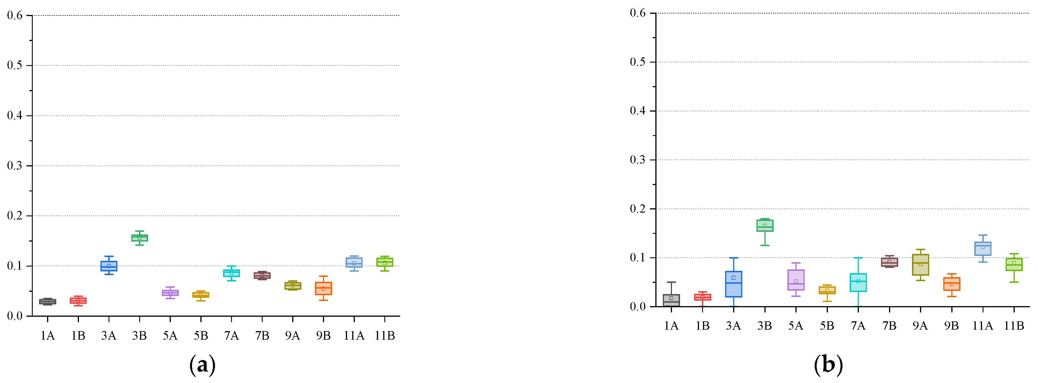
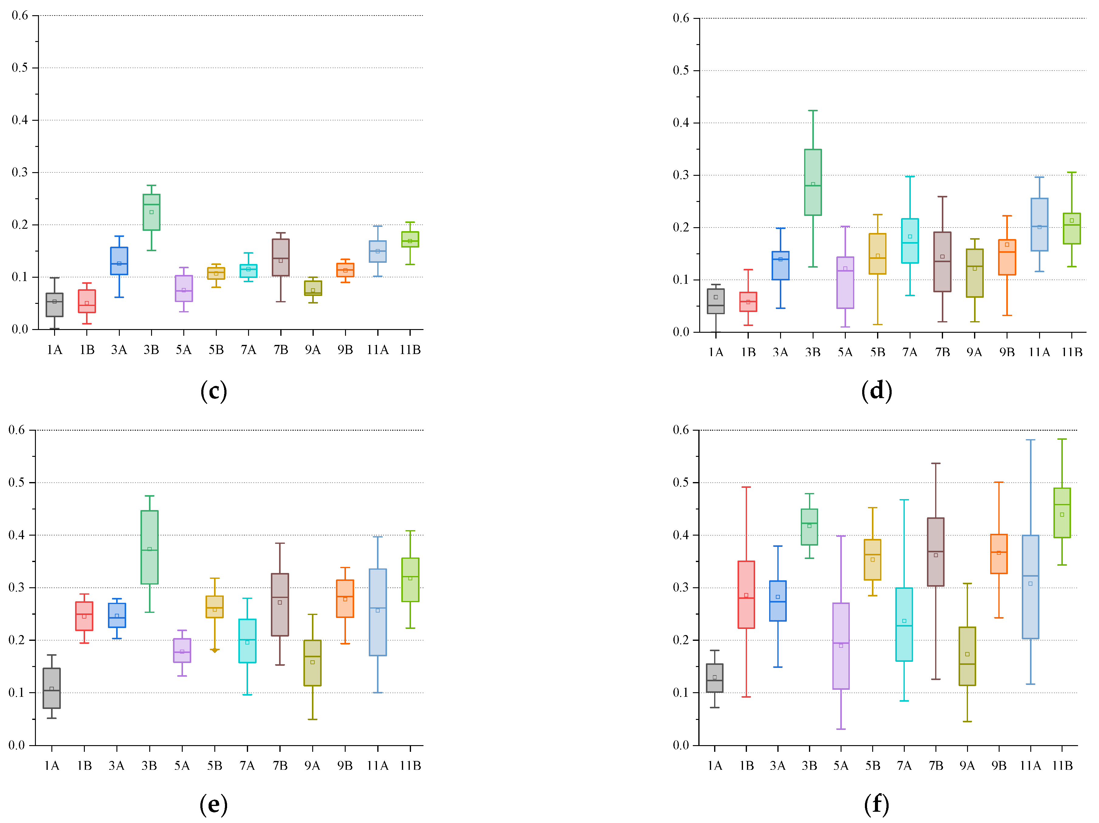
To better display the discrete distribution of the calculation results of each algorithm, we use the form of box plots for display. We selected twelve representative calculation instances (1A, 3A, 5A, 7A, 9A, 11A, 1B, 3B, 5B, 7B, 9B, 11B); each calculation example was independently run thirty times under each algorithm, and the data from those thirty runs are displayed in the form of box plots, as shown in Figure 13.

The upper line of the box is the upper 1/4 median $Q_1$, the middle line of the box is the median $Q_2$, the lower line of the box is the lower 1/4 median $Q_3$, and the top and bottom short lines represent the largest observations. For the observation of the box plot, first, the value of the box must be within the convergence range to indicate that the individual has converged. Second, smaller box lengths are better, and mean that the individuals are more concentrated, leading to relatively more stable algorithm performance. In addition, the distribution of individuals can be seen from the position of the median line. Finally, the number of extremely discrete individuals is as small as possible.

It can be seen from Figure 13 that NSGA-III can produce the most promising non-dominated solution. The individuals in the solution are relatively concentrated, the algorithm’s performance is stable, the convergence is good, and the robustness is strong.

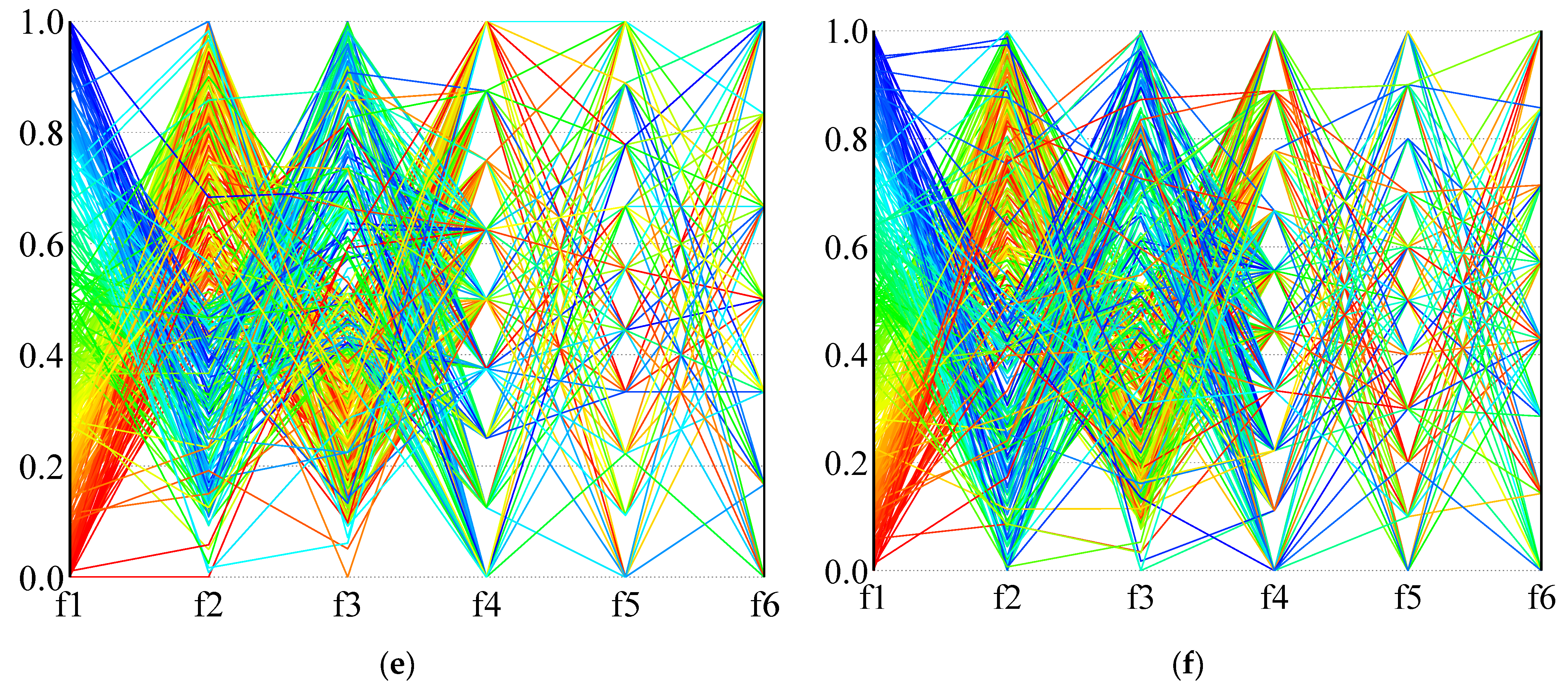
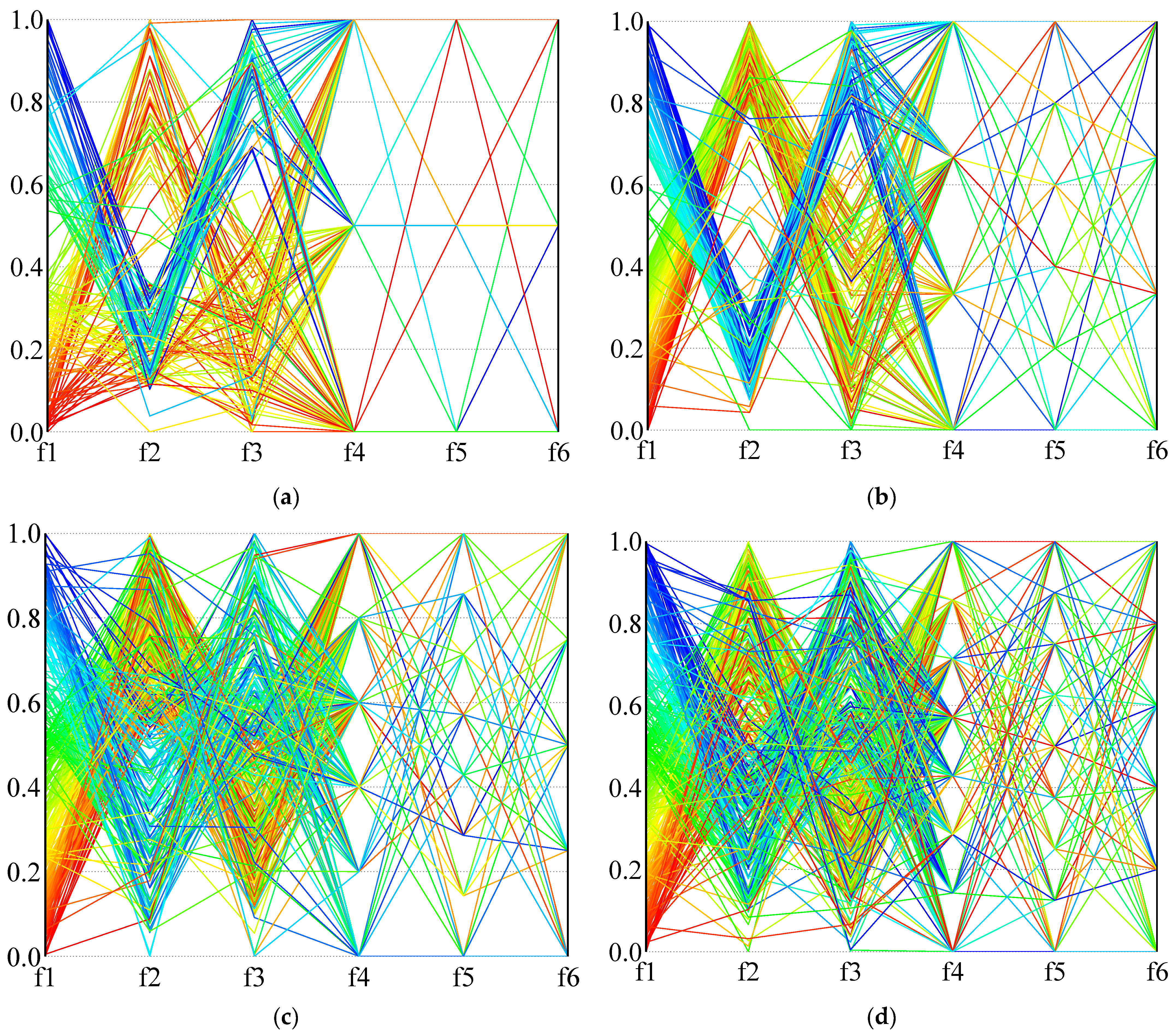
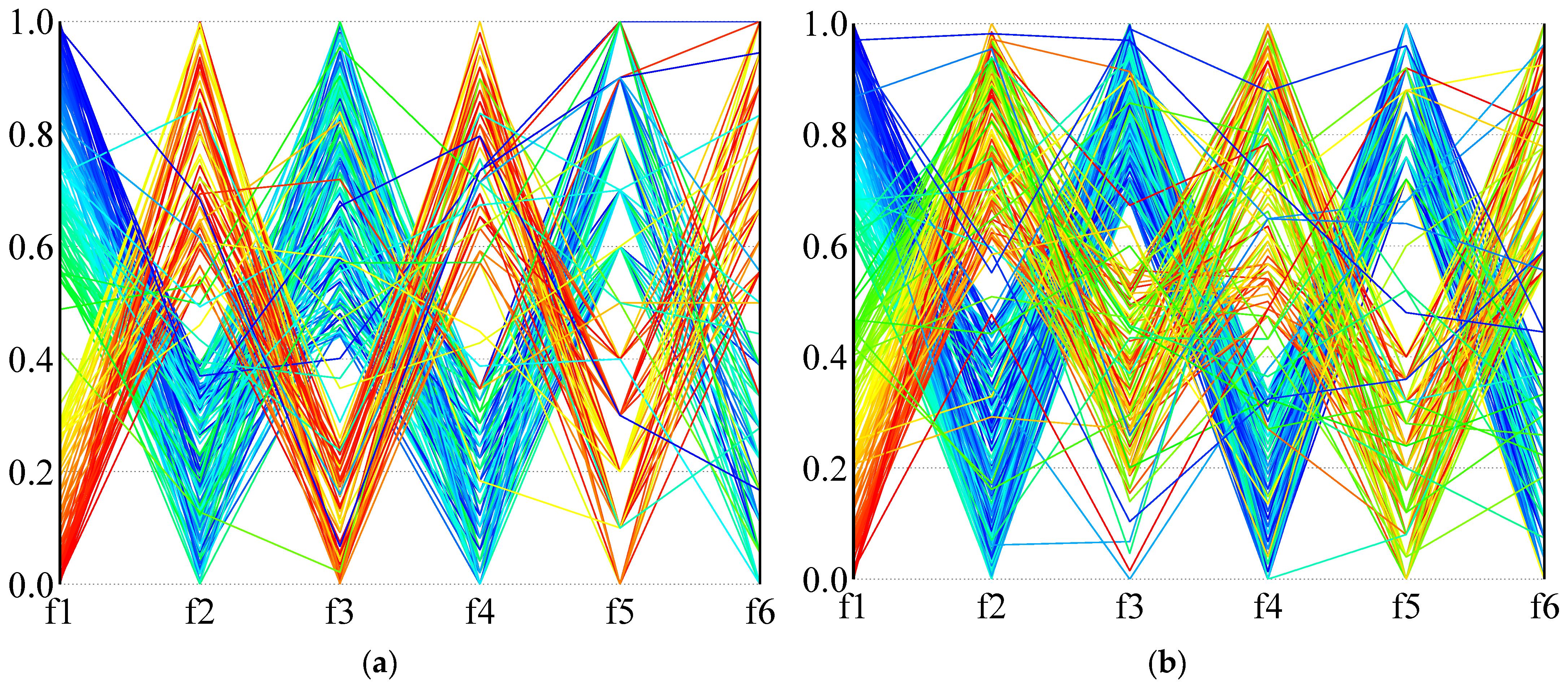
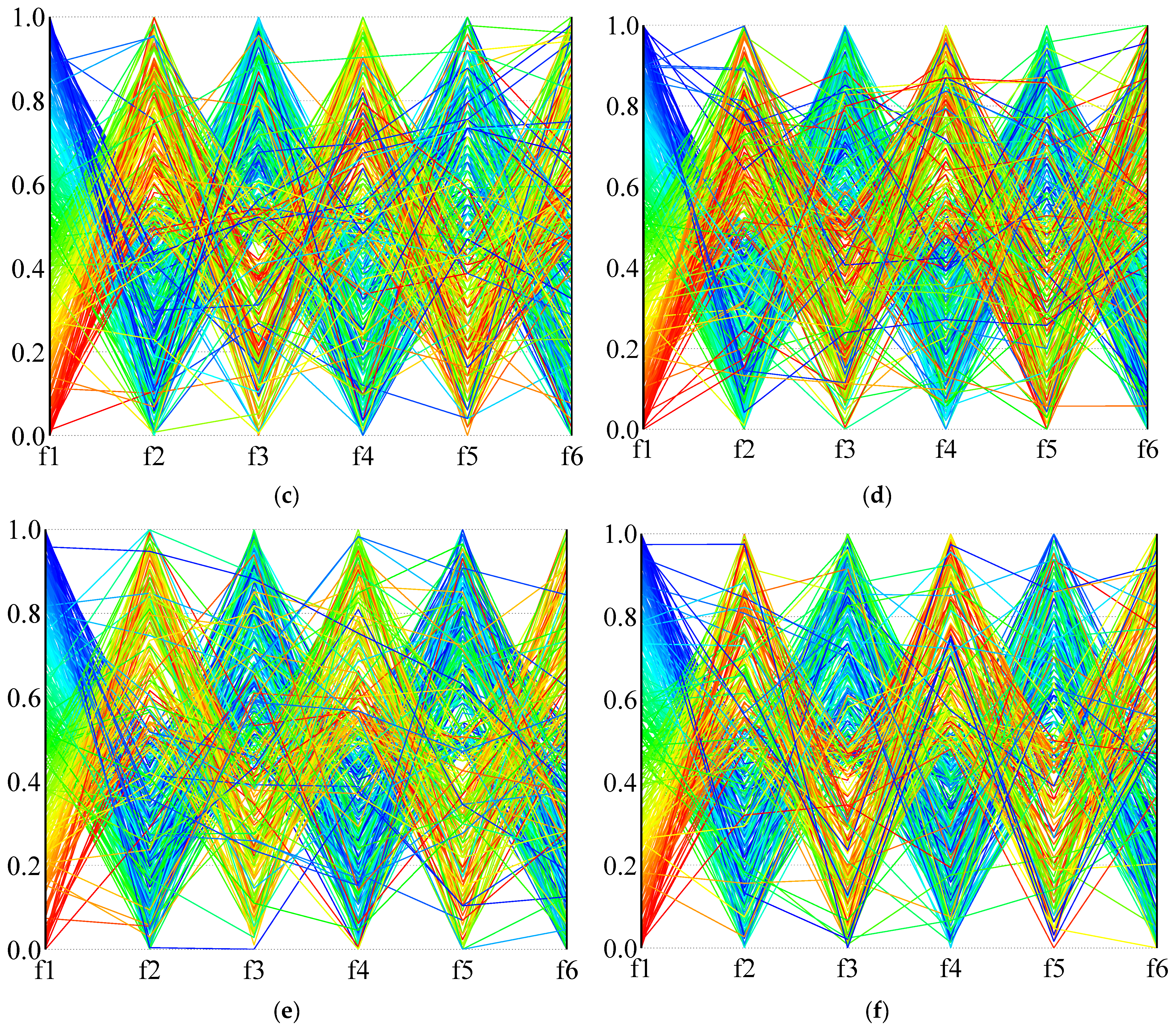
In order to more intuitively describe the distribution of the solution in the high-dimensional objective space, Figure 14 and Figure 15 use parallel coordinates to plot the non-dominated solutions generated by the different algorithms used in the two calculation examples (1A and 24B). For each algorithm and instance, we collected the non-dominated solutions (30 × 100 = 3000 solutions in total) generated by thirty independent runs and removed the dominated solutions. As the value of each objective function is not in the same dimension, the value of each dimension of the solution space is normalized, and the value in the figure is the normalized result. Figure 14 is the result of calculation example 1A, and Figure 15 is the result of calculation example 24B. It can be seen from the results that NSGA-III-L and NSGA-III-NL show the most vital convergence, especially in the face of complex situations (instance 24B), and result in better non-dominated solution sets. Although NSGA-II is not as convergent as NSGA-III when dealing with many-objective problems, it can provide a clear compromise solution. When RWGA deals with multi-objective problems, finding a convergent compromise solution is difficult. The results in Figure 14 and Figure 15 are consistent with the results in Table 9, Table 10 and Table 11. When dealing with many-objective problems, the NSGA-III and NSGA-II methods can cover the objective space more completely and consistently than RWGA, and provide clearer compromise solutions for decision-makers to choose from.

In summary, considering the different evaluation indexes of the algorithm’s distribution, convergence, and versatility, it is impossible to find an algorithm that performs perfectly under every index. Although the comprehensive performance of NSGA-III is more outstanding in multiple calculation examples, it is not the only perfect algorithm. The results show that our proposed variant based on NSGA-III can provide decision-makers with excellent and satisfying diverse non-dominated solutions, especially when dealing with high-dimensional multi-objective container stowage planning problems. This algorithm can achieve a better compromise between convergence and diversity. In practice, therefore, we recommend using NSGA-III-L.

6. Conclusions

As the container stowage plan often represents the major bottleneck in container transportation, effective methods to solve the problem of container stowage planning can ensure safety and improve economic benefits. Our study simultaneously considers ship stability and the number of container shifts and proposes an MaO-CSPP with six objective dimensions. This study mainly involves two categories, namely, ship stability and the number of shifts, and contains six specific objectives. To solve this problem, we added local search and neighborhood operators based on NSGA-III and designed a variant of NSGA-III. These variants can provide decision-makers with better non-dominated solutions. To evaluate the performance and effectiveness of the algorithm, we generated 48 calculation examples based on the EDI files of actual production and operation. We carried out extensive experiments on each algorithm. The experimental results verify the effectiveness of the algorithm. Compared with other algorithms, we found that the comprehensive performance of the algorithm is more prominent and that good results can be achieved in more calculation examples. Therefore, this algorithm is the most suitable for handling MaO-CSPPs.

The research in the present study mainly involves the coordinated optimization of ship bay stowage and container yard retrieval. In further research combining the coordinated optimization of yard pre-marshalling and crane schedules can allow more realistic problems to be solved. In addition, this research on many-objective visualization provides decision-makers with a more intuitive form in which to display result, allowing them to quickly choose among many compromise solutions according to different needs and based on different preferences.