Article

Hydrodynamic Analysis of Tidal Current Turbine under Water-Sediment Conditions

State Key Laboratory of Fluid Power and Mechatronic Systems, Zhejiang University, Zheda Rd.38, Hangzhou 310027, China
*
Author to whom correspondence should be addressed.
J. Mar. Sci. Eng. 2022, 10(4), 515; https://doi.org/10.3390/jmse10040515
Submission received: 6 March 2022 / Revised: 25 March 2022 / Accepted: 28 March 2022 / Published: 8 April 2022
(This article belongs to the Section Ocean Engineering)

Abstract

:
The rivers connecting oceans generally carry sediment due to water and soil losses in China. Additionally, the maximum sediment concentration is 300 g/L, which is much higher than that of other countries. It is unknown whether seawater with sand particles will affect the power of tidal current turbine blades. It is therefore necessary to study the capture power of tidal current turbines in the water-sediment environment. In this study, the blade was divided into a number of transversal airfoil elements based on the blade element theory. The CFD-DPM model was employed to study the lift and drag coefficients of airfoil under multiphase flow, and the fluid–particle interaction was considered. The accuracy of this presented model was assessed using the experimental data of a 120 kW tidal current turbine in a water-sediment environment. Good agreement between the predictions and experimental data was observed. The effect of particle properties on the lift coefficient and the drag coefficient of airfoil were investigated in detail. Furthermore, the 120 kW tidal current turbine power was calculated based on the Blade Element Momentum theory under different particle concentrations. The results show that small diameter particles can improve the tidal current turbine power and the large diameter particle can reduce the power.

Graphical Abstract

1. Introduction

Tidal energy has the advantages of abundant reserves, high energy density, and strong predictability [1]. In China, there is an abundance of tidal energy resources, and the estimated power is up to 14,000 MW [2,3]. Large-scale tidal current turbine and turbine arrays have become a trend in research, which puts forward strict requirements for the efficiency of blades [4,5,6,7]. However, due to the serious water and soil loss in river basins, a lot of sediment is brought into the channel, so the rivers generally carry this sediment [8]. Additionally, the particle properties are greatly diverse in different sea areas; the maximum particle concentration can reach 300 g/L in the Yellow River [9,10,11]. Part of the sea sediment is derived from rivers; the concentration of suspended sand reaches 5.522 g/L in the Zhoushan sea area. The maximum suspended sand concentration is 10 g/L in Aojiang coast, and the maximum particle concentration near the bottom is 20 g/L [12,13]. It is unknown whether the interaction between seawater and sand will change the flow behaviors around the blade and lead to a change in the blade capture power. It is therefore particularly necessary to study the hydrodynamic performance of tidal current turbine blades in a water-sediment environment.
Fraenkel and Ng et al. [14,15] point out that the roughening of tidal current turbines due to particle impacts or cavitation is a potential performance problem. Batten et al. [16] investigated the effect of increasing blade roughening on blade power based on the Blade Element Momentum (BEM) theory. Soonseok et al. [17] show that the modified wall-function approach can precisely predict the roughness effect on the performance of tidal current turbines. Walker et al. [18] tested the lift and the drag coefficient of the NACA airfoil section with both clean and roughened conditions using a wind tunnel. Additionally, they used a towing tank to test a model rotor in different surface conditions. These studies demonstrate that the power coefficient will decrease with increasing blade roughness.
Most studies have focused on the power loss due to the increase in blade roughness caused by the impact of sand particles. Almost no study has been carried out on the hydrodynamic performance of tidal current turbine under water-sediment conditions, and a few researchers have performed comprehensive simulations regarding to the effects of various variables on blade power under multiphase flow. This is because a high concentration of 300 g/L of sediment exists in China, which is greatly different from that of other countries. For example, the Amazon, the world’s largest river, has an average sediment concentration of 0.13 g/L. The longest river in Europe, the Volga, has an average sediment concentration of 0.11 g/L [9,11]. Additionally, most of the experimental data are based on wind tunnel or towing tank experiments, which lack the verification of experimental data in realistic sea environments.
In order to study the hydrodynamic performance of the blade under multiphase flow, both experiments and numerical simulation methods can be useful tools. However, it is difficult to capture flow characteristics considering all influencing factors using experiments. Therefore, many numerical calculation approaches to predicting flow characteristics have been proposed. The Euler–Euler model and the Euler–Lagrange model are the most common models.
In the Euler–Euler model, both particles and liquid phases are treated as continuous phases according to Navier–Stokes equations, but additional models are needed to define the shear stress and the pressure of the solid phase [19]. It is convenient and widely used in research, but it cannot obtain true particle motion and flow characteristics due to the constitutive relations for describing solid stress [20]. In the Euler–Lagrange model, the fluid phase is treated as continuous phase via Navier–Stokes equations and the solid phase is modeled as a discrete phase via Newton’s second law [21]. The model is able to capture the motion of every particle, and the particle–particle and particle–wall interactions can be taken into account.
Both the Discrete Element Method (DEM) and the Discrete Phase Model (DPM) are applied to track the trajectory of the particles using the Lagrange approach. The DEM considers the interaction between particles, which can be used to model a wider range of flows from low to high particle concentrations [22]. Unlike DEM, the DPM is only applied to simulate the dilute particle flow, because it is based on the assumption that the interaction between particles is negligible [23]. However, the concept of a particle parcel is applied in DPM the model, such that one particle replaces all particles with the same properties in a parcel, which will be beneficial for faster calculation and cost less computer resources [24]; as a result, the DPM is more appropriate for the dilute phase to capture particle physics. Most of these numerical simulation methods are carried out in closed environments, such as fluidized beds pipeline conveying. Further study is required to determine whether the simulation methods are suitable for open environments.
Airfoil is the key element in tidal current turbine blades, and the performance of the airfoil can significantly affect the performance of the tidal current turbine blade. In this research, based on blade element theory, the tidal current turbine blade was divided into a number of transversal airfoil elements. The Computational Fluid Dynamics-Discrete Phase Model (CFD-DPM) model was employed to simulate the lift and the drag coefficients of airfoil under multiphase flow. Two-way coupling was selected considering the particle–fluid interaction. First, the governing equations for liquid flow, particle, and the basic concept of airfoil are given [25]. Then, the accuracy of the CFD-DPM model was validated with the corresponding experiments of 120 kW tidal current turbine in realistic sea environments. Furthermore, the lift and the drag coefficients of airfoil under different particle properties were investigated. In the process of revealing the cause of hydrodynamic performance change, the particle velocity and the fluid velocity with and without particles along the same particle trajectory were analyzed. The analysis method is to analyze the influence of particles on fluid velocity first, and then the change in lift/drag coefficient caused by the fluid velocity is analyzed. Finally, the 120 kW tidal current turbine power was calculated based on the Blade Element Momentum theory under different particle concentrations. The analysis process and results can further provide suggestions on the field-site selection for tidal current turbine and the blade design for maintaining the high efficiency of blades.

2. Mathematical Model

2.1. Particle Phase Model

In the CFD-DPM model, the particle is treated as a discrete phase, so the governing equation of particle motion is described according to Newton’s second law, written as follows [26,27]:
d ν P d t = ( ρ P ρ f ) g ρ P + f D + f LS + f P + f add + f C
where ν P is the particle velocity and ρ P and ρ f represent the particle density and the fluid density, respectively.
The drag force f D is the most dominant force acting on the particle, as shown in the following equation [28]:
f D = 3 ρ f 4 ρ P d P C D ( U f ν P ) U f ν P
The added force f P is caused by the pressure gradient in the flow field and is expressed as:
f P = ( ρ f ρ P ) ν P U f x
The virtual mass force f add , which is the added mass force due to the acceleration of fluid phase around a particle, is given by the following [29]:
f add = 1 2 ρ f ρ P d d t U f ν P
The lift force f LS is caused by the fluid transverse velocity gradient (shear layer flow), which is expressed as follows [30]:
f LS = 2 k U f 1 / 2 ρ f d i j ρ P d P ( d l k d k l ) 1 / 4
The particle–particle force f c includes the normal force f cn and the tangential force f ct , as the following equation shows [22]:
f c = f cn + f ct
k is constant, k = 2.594 , d i j is the fluid deformation rate tensor, d P is the particle diameter, and U f is the velocity of fluid.
For a smooth spherical particle, the fluid drag coefficient C D proposed by Morsi and Alexander is adapted as follows [28]:
C D = a 1 + a 2 R e p + a 3 R e p 2
where a 1 , a 2 , and a 3 are constants, which vary with respect to the Reynolds number.
For non-spherical particles, the fluid drag coefficient C D is given as follows [31]:
C D = 24 R e p ( 1 + b 1 R e P b 2 )   +   b 3 R e p b 4 + R e p
where b 1 , b 2 , b 3 , and b 4 are parameters related to particle shape:
b 1 = exp ( 2.3288 6.4581 ϕ + 2.448 ϕ 2 )
b 2 = 0.0964 + 0.5565 ϕ
b 3 = exp ( 4.905 13.8944 ϕ + 18.4222 ϕ 2 10.2599 ϕ 3 )
b 4 = exp ( 1.4681 + 12.2584 ϕ 20.7322 ϕ 2 + 15.8855 ϕ 3 )
R e P is the particle Reynolds number, as shown below [32]:
R e p = ρ f d P μ f U f ν P
where μ f is the fluid dynamic viscosity.
The turbulent diffusion of the suspended sediment reaches a temporary equilibrium with the gravity of suspended sediment, so the gravity is negligible; since the particle diameter is greater than 10 µm, the Saffman lift force can be neglected. Additionally, as the ratio of fluid density to particle density is low, neither the pressure gradient force nor the virtual mass force is taken into account.

2.2. Fluid Phase Model

In the CFD-DPM model, the fluid flow is treated as a continuous phase, so the governing equation of the fluid is described using the continuity and momentum conservation equations, as shown below:
t ( ρ f ) + ( ρ f U f ) = 0
t ( ρ f U f ) + ( ρ f U f U f ) = P + ( R f ) + ρ f g + f Pf
where P is the fluid pressure gradient.
The volumetric fluid–solid interaction force f Pf proposed by Zhou is adopted [25,33]:
f Pf = 1 V cell i = 1 K C ( f d , i + f LS , i + f add , i )
where K C is the number of particles in one of the considered computational cell and V cell is the volume of the computational cell.
As the object of this study includes the airfoil lift and the drag coefficients, the influence of particles on the fluid is taken account in the momentum equation of the fluid, and two-way coupling is used.
The stress tensor R f includes two parts, viscous stress and Reynolds stress, which are given as [24]:
R f = μ f U f + ρ f τ
where τ represents the Reynolds stress, which is expressed as
τ = 2 ρ f η t S 2 3 μ f ρ f I
S = 1 2 ( U f + ( U f ) T )
where η t stands for the turbulent viscosity and I is the unit tensor.
Since flow variables changes significantly very close to the wall, an accurate fluid flow solution in the region is needed [34,35]. There are two approaches to simulating the fluid flow near the wall. In the first approach, the wall functions are used to model the viscous sublayer and the buffer layer. In the second approach, modified turbulence models are adopted to resolve the fluid flow field, is more accurately predicts the fluid flow near the wall [34], so the SST k-ω model is employed to compute Reynolds stress in the Reynolds-averaged NS equations in the following study, which are given as:
t ( ρ f k )   +   x i ( ρ f k u i ) = x j ( μ f + μ t σ k ) k x j   +   G k Y k + S k
t ( ρ f ω )   +   x i ( ρ f ω u i ) = x j ( μ f + μ t σ ω ) ω x j   +   G ω Y ω + D ω + S ω
where u i is the velocity component in i the direction, x i and x j are the spatial coordinates, σ k and σ ω are the turbulent Prandtl numbers for k and ω , G k is the turbulent production, G ω is the specific dissipation production, Y k and Y ω are the diffusion production, D ω is the cross-diffusion term, and S k S ω are the user-specified source terms [36].

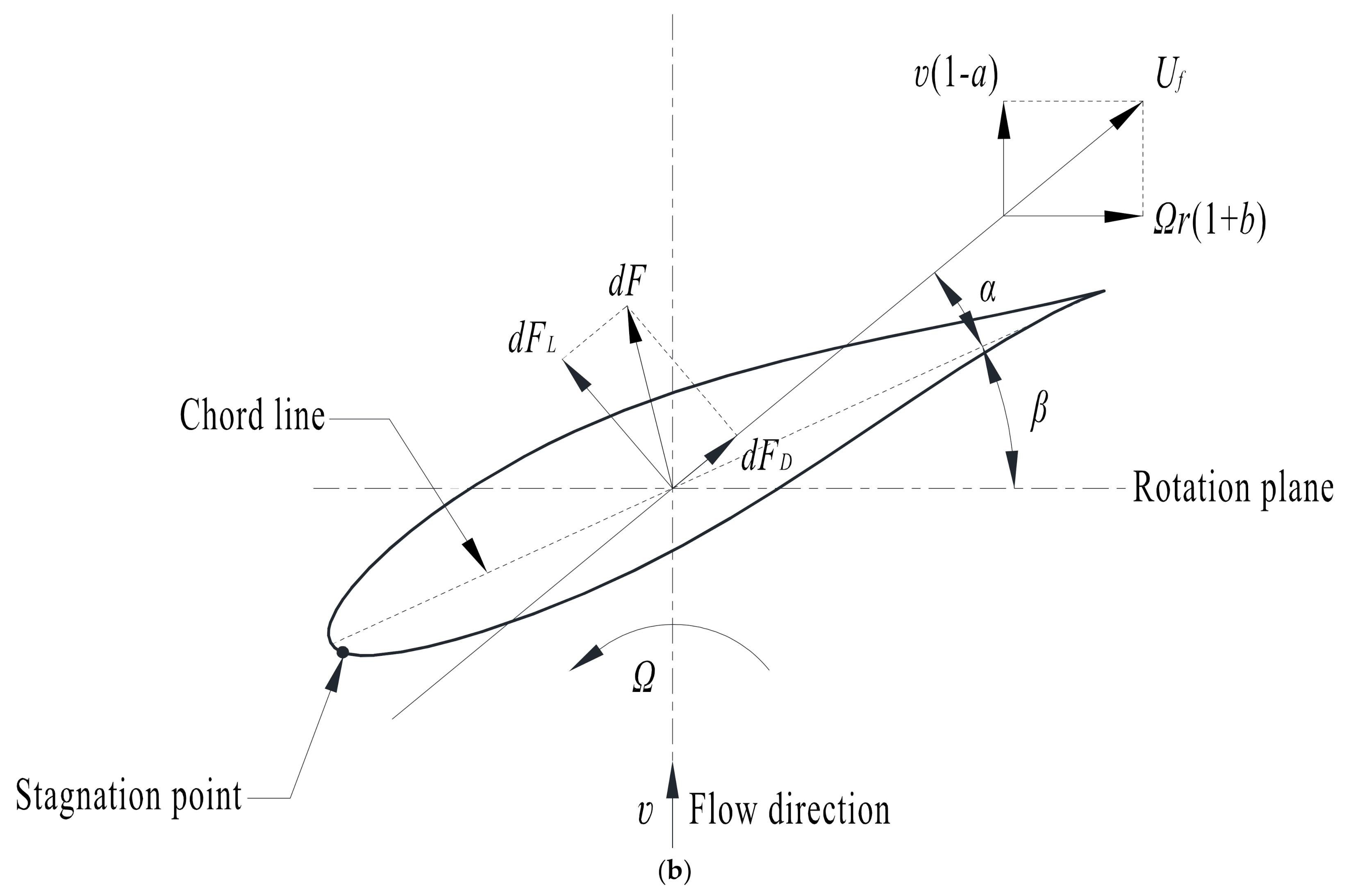
2.3. Blade Element Momentum (BEM) Theory
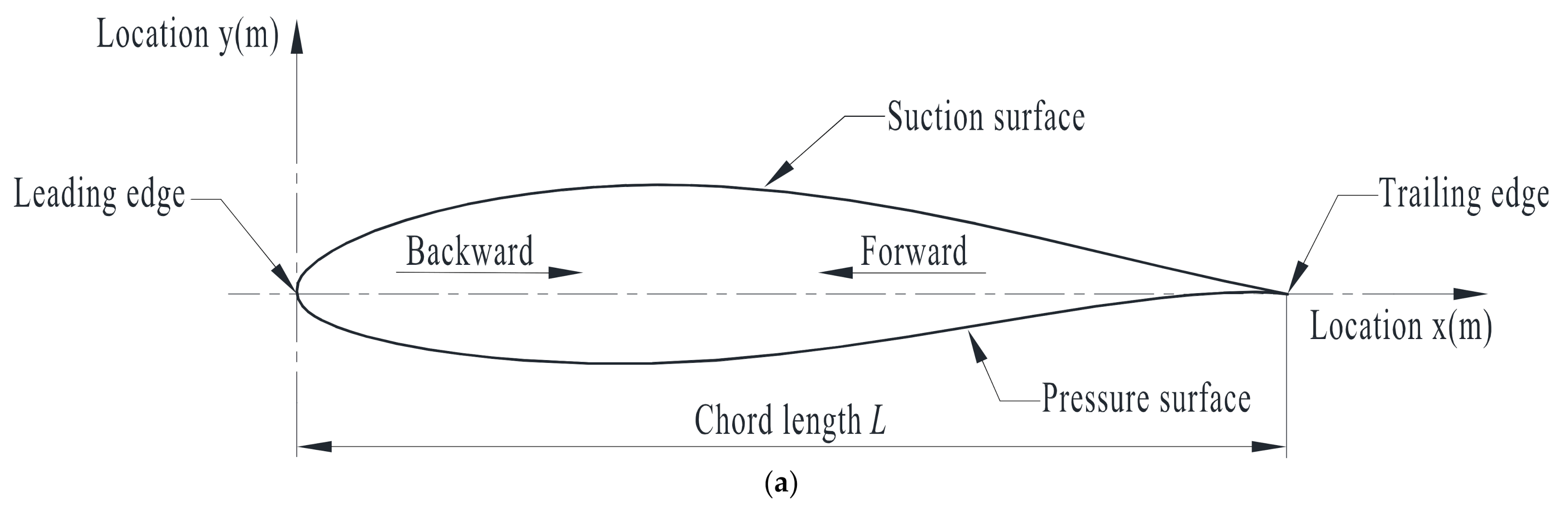
According to blade element theory [37,38], the blade of tidal current turbine is divided into a number of transversal elements, placed along the blade. Figure 1 shows the geometric and the hydrodynamic parameters of the airfoil element.
Consider that the turbine is situated in a tidal flow of v velocity, Ω is the turbine rotating speed, and U f is the relative velocity of tidal current, which is expressed as follows:
U f = ( 1 a ) 2 υ 2   +   ( 1 + b ) 2 2 r 2
where r is the radius of the local blade element and a and b denote the axial and the tangential flow induction factors, respectively [39,40,41].
The angle between the relative velocity of tidal current U f and the chord line is defined as the angle of attack α, β is the twist angle, and φ is the flow angle, which is given by:
φ = α + β   = tan 1 1 a 1 + b 1 λ r
where λ r is the local tip speed ratio.
According to the blade element theory, the thrust T and torque M on a span-wise length d r of the rotor (each blade) can be calculated by [39,40,41]:
d T = N d F L cos φ + d F D sin φ = 1 2 N ρ c U f 2 C L cos φ + C D sin φ d r
d M = N r d F L sin φ d F D cos φ = 1 2 N ρ c U f 2 C L sin φ C D cos φ r d r
where c is the local chord length and N is the number of blades of the tidal current turbine.
According to the momentum theory, the thrust T and torque M are given by [39,40,41]:
d T = 4 ρ π v 2 a 1 a r d r
d M = 4 ρ π v 1 a b r 3 d r
Therefore, the axial flow induction factor can be calculated by combining Equations (24) and (26) as
a = N c C L cos φ + C D sin φ 8 π r sin 2 φ + N c C L cos φ + C D sin φ
The tangential flow induction factor can be calculated by combining Equations (25) and (27) as
b = N c C L sin φ C D cos φ 8 π r sin φ cos φ N c C L sin φ C D cos φ
The chord length and twist angle can be given as
c r = 8 π r a N C L ( 1 a ) · sin 2 φ cos φ
β r   = tan 1 1 a 1 + b 1 λ r α
The Prandtl’s approximation method is adopted considering the blade tip and blade root losses, which are expressed as follows [39]:
F = F t F r = 2 π cos 1 exp N 2 R r R sin φ 2 π cos 1 exp N 2 r r h r h sin φ = 4 π 2 cos 1 exp N 2 R r R sin φ cos 1 exp N 2 r r h r h sin φ
where F is the Prandtl correction factor, Ft is the tip loss factor, Fr is the root loss factor, and r h is the radius of the hub.
The axial flow induction factor, tangential flow induction factor, chord length, and twist angle are modified as:
a = N c C L cos φ + C D sin φ 8 π r F sin 2 φ + N c C L cos φ + C D sin φ
b = N c C L sin φ C D cos φ 8 π r F sin φ cos φ N c C L sin φ C D cos φ
c r = 8 π r ( 1 a F ) N C L ( 1 a ) · sin 2 φ cos φ
β r = tan 1 1 a 1 + b 1 λ r   α

2.4. Airfoil

The airfoil is the section cut out from the blade along the incoming flow direction, and NACA airfoils are the most commonly used airfoils for tidal current turbine blades. The Airfoil is the key element in the tidal current turbine blade, and the performance of the airfoil can significantly affect the performance of the tidal current turbine blade. The blade power is positively correlated with the lift coefficient of the airfoil and negatively correlated with the airfoil drag coefficient.

2.4.1. Airfoil Lift Coefficient

Dimensionless lift coefficient of airfoil [42,43]:
C L = d F L 1 2 ρ f U f 2 c d r = f ( R e , α )
R e = ρ f U f c μ f
The airfoil lift comes from the pressure difference between the suction surface and the pressure surface, which is caused by the fluid velocity difference between the suction surface and the pressure surface. On the suction surface, the fluid velocity accelerates to the maximum from the zero of the stagnation point and then decreases. On the airfoil pressure surface, the fluid velocity decreases at first and then increases.
The lift coefficient can be reflected by the degree of change of the fluid velocity at the same streamline position. The more the fluid velocity changes at the same streamline position, the greater the lift coefficient is.

2.4.2. Airfoil Drag Coefficient

Dimensionless lift and drag coefficients of airfoil [42,43]:
C D = d F D 1 2 ρ f U f 2 c d r = f ( R e , α )
The drag is caused by the viscosity of the fluid, which includes the frictional drag and the pressure drag (the pressure drag formed by the pressure difference between the leading and the trailing of the airfoil). With the increase in the angle of attack, the flow separation is promoted, and the separation point moves forward. The pressure in the vortex region decreases, the pressure drag increases, and the drag coefficient increases. As the relative velocity increases, the flow separation is inhibited and the pressure drag decreases. Additionally, it was determined through experiments that with the increase in the relative velocity, the frictional drag increases and the frictional drag coefficient decreases. As a result, with the increase in relative velocity, the drag coefficient decreases.

3. Computational Details

3.1. Case Description

In the present work, ANSYS ICEM was adopted to perform geometric modeling and mesh generation [44]. The commercial software ANSYS FLUENT was the CFD solver used for numerical simulation [45]. The experiment data of 120 kW tidal current turbine were employed in this work to investigate the hydrodynamic performance of blade under water-sediment conditions. A 120 kW tidal current turbine was used carried out sea trials in Zhoushan (Figure 2), and it has been operating for 4 years in water-sediment conditions (Figure 3). Figure 4 shows the 120 kW tidal current turbine blade profile, which contains 30 blade elements; the airfoil element at the tip is named “airfoil 30”, and the others are named in sequence. The 120 kW tidal current turbine blade fundamental parameters are listed in Table 1. Additionally, the 120 kW tidal current turbine blade geometrical parameter distributions along the blade are listed in Table 2. The suspended sediment in the Zhoushan sea area is composed of heterogeneous sand particles, and the logarithm of natural sediment particle size obeys normal distribution. Table 3 lists the details of the particle size distribution in Zhoushan. In order to study the hydrodynamic performance of the blade under a multiphase flow, the 120 kW tidal current turbine blade is divided into a number of transversal airfoil elements based on the blade element theory in the following study.

3.2. Model Description and Boundary Conditions

The domain and boundary conditions used for the simulation are shown in Figure 5. To avoid any spurious influence from the boundary surfaces, the domain extends 12.5 chord lengths upstream of the airfoil and 16 chord lengths downstream. The NACA63-xxx airfoil is chosen for its high lift–drag ratio when used on the 120 kW horizontal axis marine current turbine. The particle injection surface is a virtual surface established in ANSYS FLUENT, and a uniform grid can be obtained by setting the sampling density of the edge as 1/120 chord lengths. The particle injection surface is six chord lengths upstream of the airfoil, where the effect of the airfoil on the fluid velocity can be ignored. The length of the particle injection surface is set as 10 chord lengths, and the lift and the drag coefficients no longer change with further increase of the length of the injection surface.
In the simulation, a uniform velocity is set at the inlet, and particles are injected with the same velocity as the fluid at the particle-injection surface. Hydrostatic pressure is specified at the outlet, and a no-slip boundary condition is given at the airfoil wall [46]. Particles are reflected when they impact the airfoil wall. At the outlet, particles are marked as “escaped”, and the particle parcel calculation is terminated. Table 4 lists the properties of the liquid and the particles.
Table 5 presents the simulated cases, which are assigned to research the airfoil lift and the drag coefficients under different particle properties. For the base case, the particle diameter and concentration are 500 µm and 2 g/L, respectively, and the airfoil chord, angle of attack and relative velocity of tidal current are 1 m, 6°, and 16 m/s, respectively.

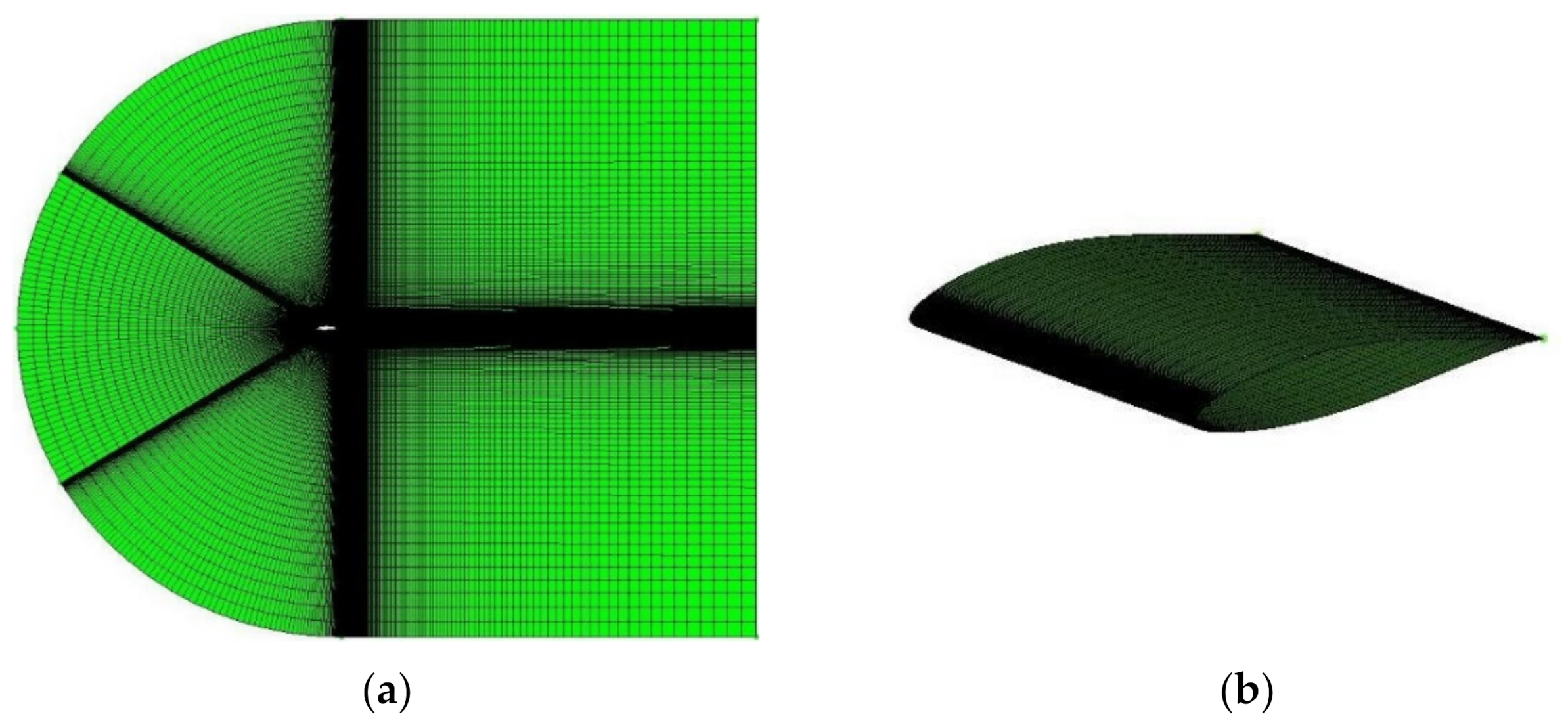
3.3. Computational Grids and Grid Independence Study

Since the flow variables such as velocity change significantly in the near-wall area [31], the computational model is hexahedrally meshed using the C-GRID topology in ANSYS ICEM, and the grids are refined in the near-wall area in order to accurately solve the near-wall fluid flow [47]. For the SST k-ω turbulence model, a very fine grid is required to maintain y+ values on the order of 1, so the size of the first cell adjacent to the wall is 0.02 mm [48].
For the accuracy of the simulation solution, the independence between the simulation results and the grid resolution needs to be verified; four grid schemes are considered to mesh the model. Table 6 shows that with the increase in the total number of cells, the lift coefficient increases and the drag coefficient decreases (the solution relative error is controlled within 0.1%). To be computationally efficient, mesh 3 is chosen in the following simulations, which is shown in Figure 6.
Table 6. Comparison of hydrodynamic performance under different grid resolutions.
Mesh NumberTotal Number of CellsLift CoefficientDrag Coefficient
11,936,7840.921970.01298
22,577,4940.925660.01287
33,239,2040.928250.01282
43,921,9140.928830.01281
Figure 6. Computational mesh used in the simulation: (a) domain volume mesh; (b) airfoil surface mesh.
Jmse 10 00515 g006

3.4. Numerical Method

The SIMPLE algorithm for pressure and velocity coupling is utilized. The pressure term is solved through standard discretization schemes. Additionally, the momentum, turbulent kinetic energy, and specific dissipation rate are handled with second-order upwind discretization schemes. The convergence of the simulation solution is set such that the residual in the control volume for each equation is smaller than 10−5. The interaction between the discrete and the continuous phases is considered, and the number of continuous phase iterations per DPM iteration is set as 10.

3.5. CFD-DPM Model Validation

3.5.1. Turbulence Model Verification

The simulated lift and drag coefficients under the SST k-ω model are shown in Figure 7. The experimental data are obtained using the wind tunnel [49]. It can be clearly observed that there is good agreement between the simulated results and the experimental data.

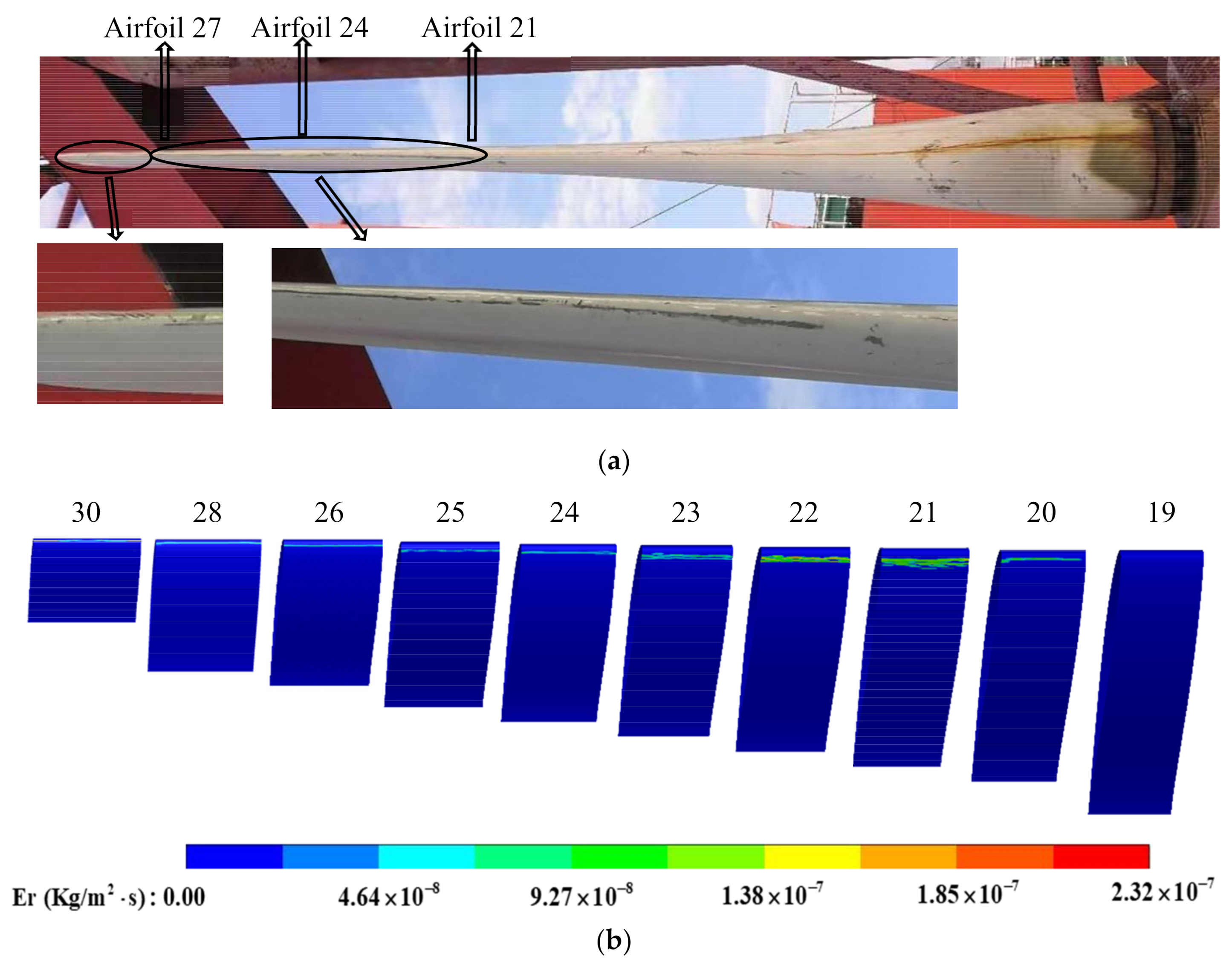
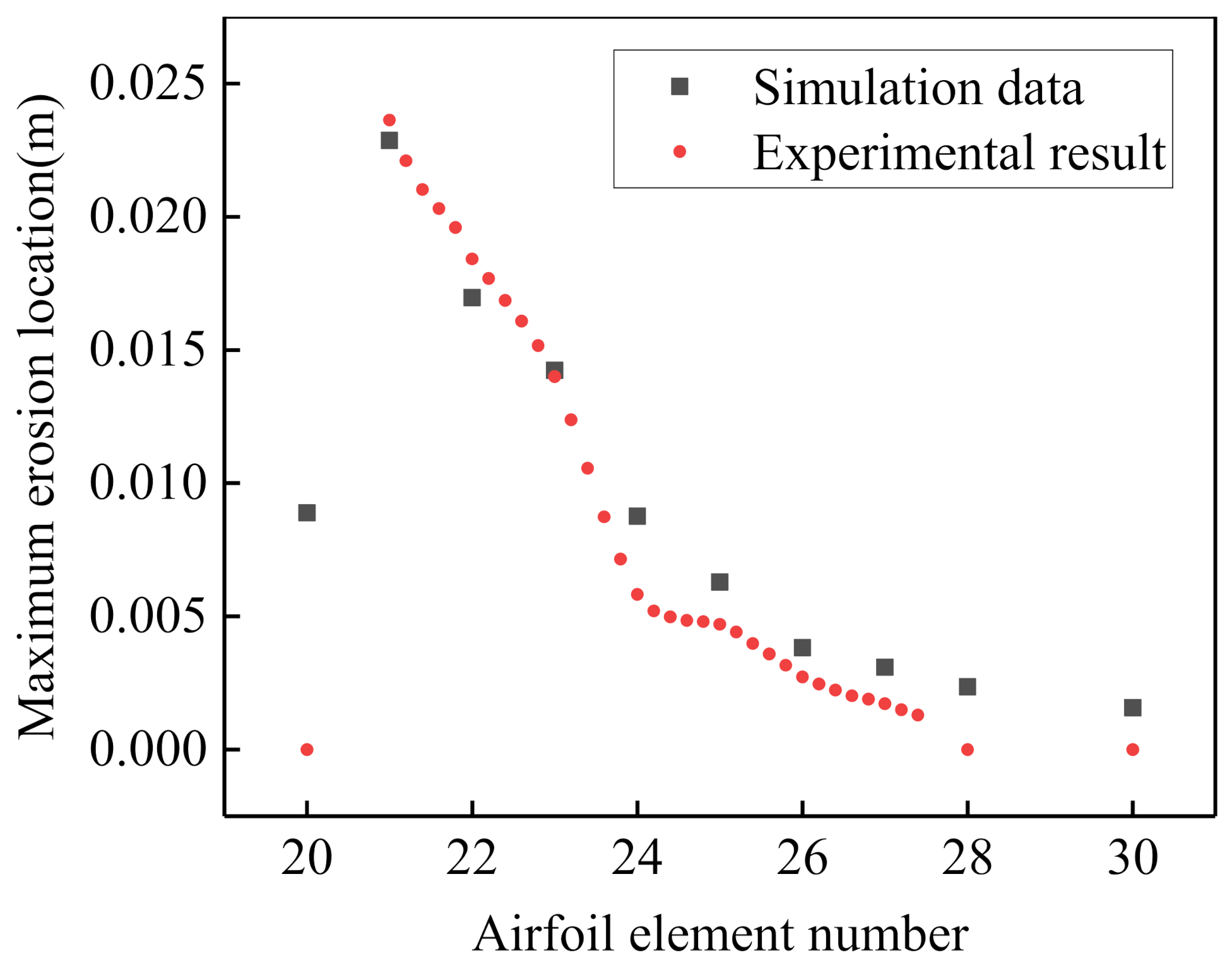
3.5.2. DPM Model Verification

In order to verify the accuracy of the DPM model, the erosion diagram of the 120 kW tidal current turbine is used, which is caused by particle impact. Figure 8a shows the actual erosion diagram of the 120 kW tidal current turbine under real sea conditions. The simulated erosion cloud diagram at 1.8 m/s with particle size the distribution taken into account is shown in Figure 8b, and Figure 9 shows the comparison of maximum erosion location of the simulation and the experiment. From the blade root to the blade tip, the maximum erosion location moves forward, which agrees well with the experimental data.

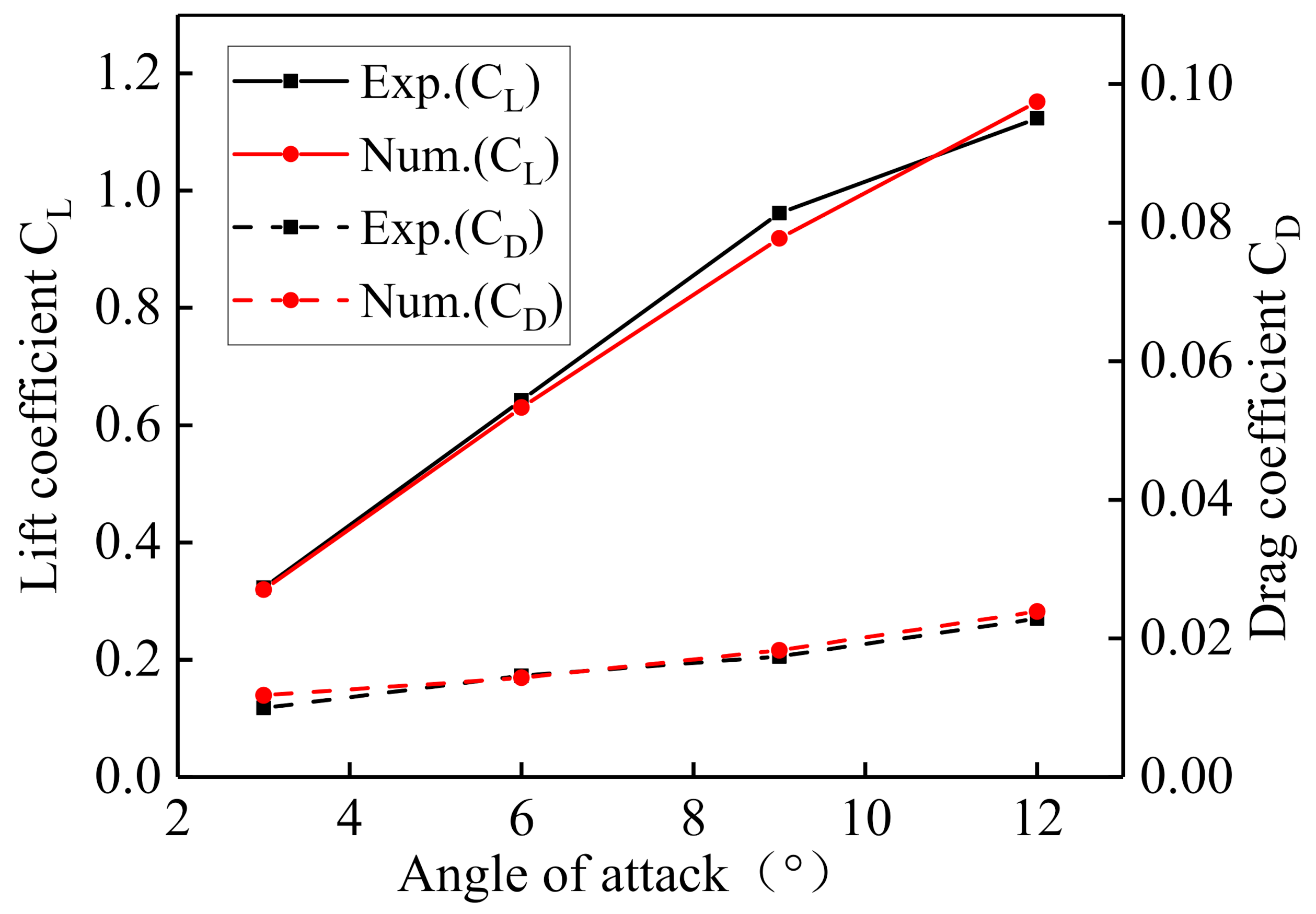
3.5.3. BEM Model Verification

The BEM model was solved using an in-house code, and the power of the 120 kW tidal current turbine was used to verify the accuracy of the BEM model. First, the lift coefficient and the drag coefficient of each airfoil were calculated using the CFD-DPM model; next, the output torque and the power of the turbine were calculated based on the BEM theory. Figure 10 shows the comparison between the simulated turbine power and the experimental data at different flow velocities. It can be found from Figure 10 that there is good agreement between the simulated turbine power and the experimental data. Thus, in the following section, the effects of particle diameter and particle concentration on the lift and drag coefficients will be assessed by using the CFD-DPM model, and the power is calculated using the BEM model.

4. Results and Discussion

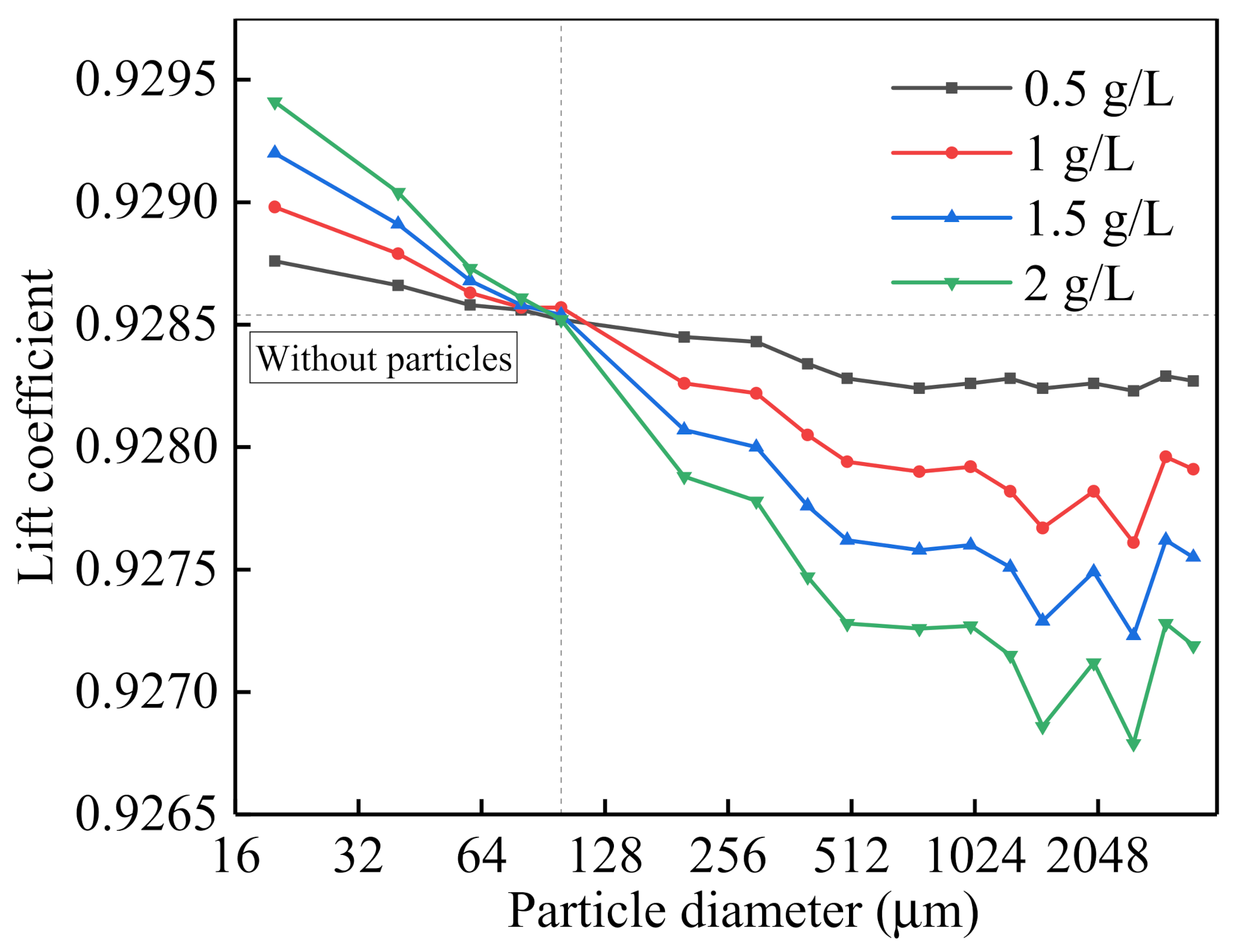
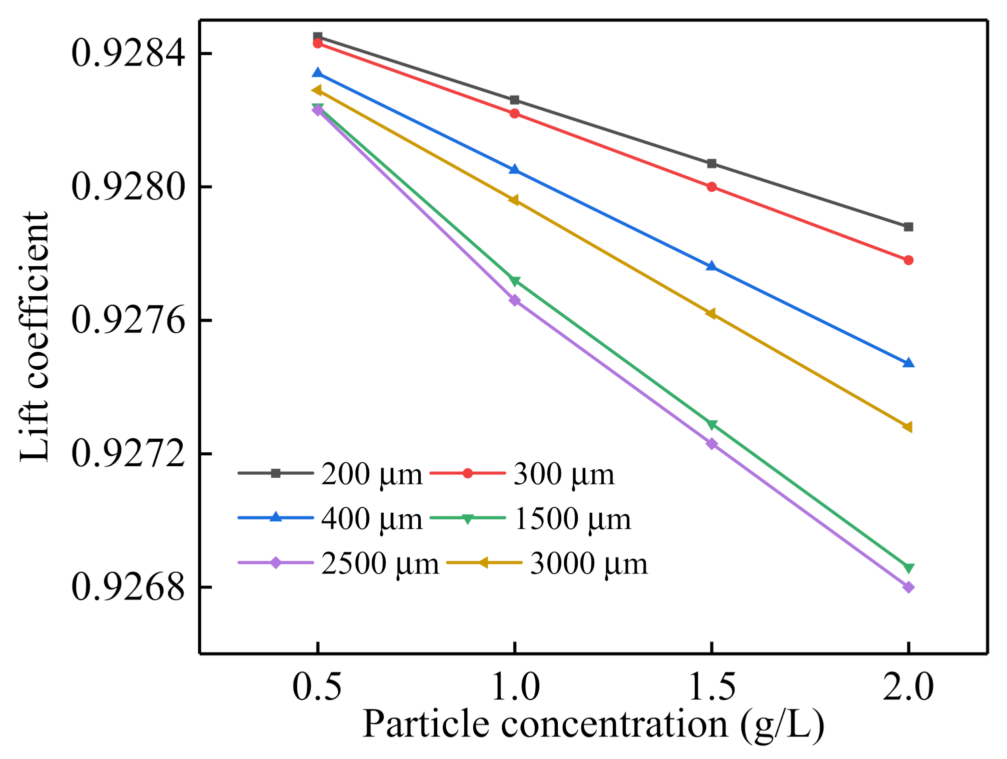
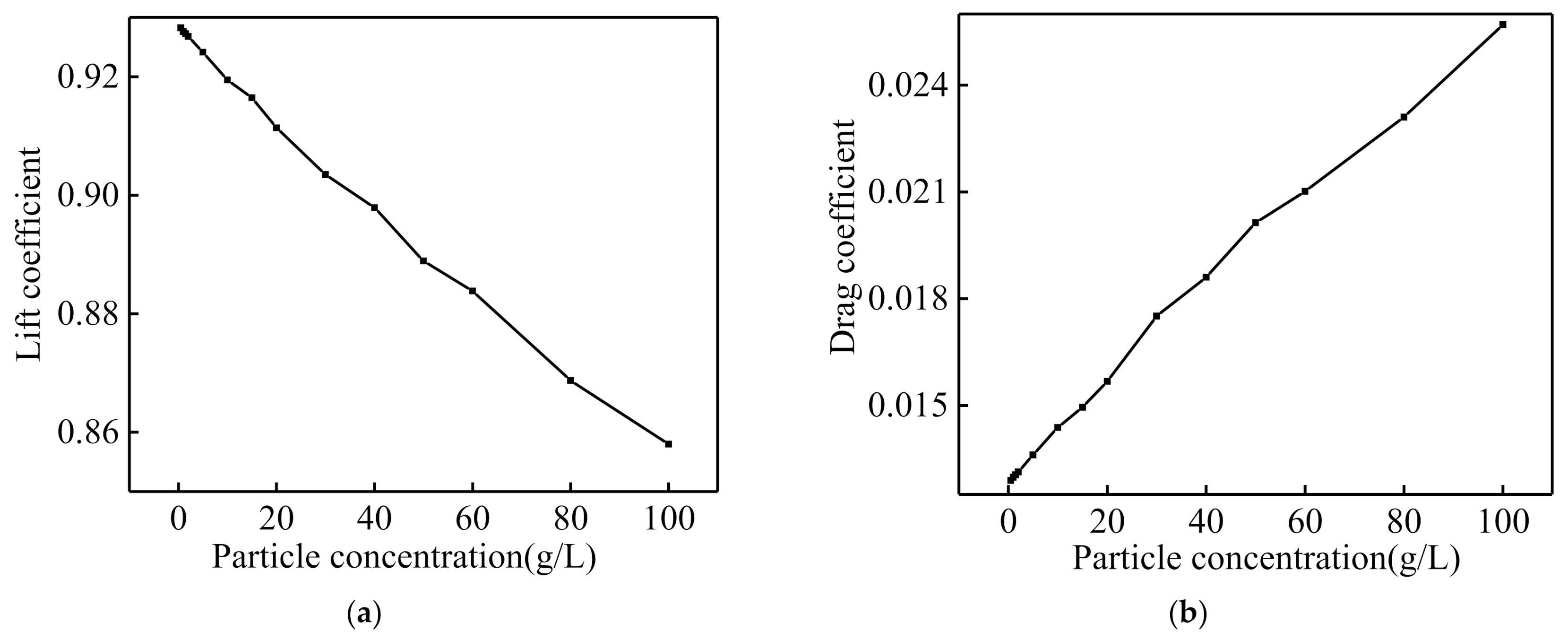
4.1. Effect of Particle Properties on Airfoil Lift Coefficient

Figure 11 shows the effect of particle properties on airfoil lift coefficient. When the particle diameter is less than 100 µm, the airfoil lift coefficient is greater than the airfoil lift coefficient without particles. The airfoil lift coefficient increases as the particle concentration increases. When the particle diameter exceeds 100 µm, the airfoil lift coefficient is smaller than the lift coefficient without particles. The airfoil lift coefficient decreases as the particle concentration increases.
Figure 12 displays the particle trajectories and the fluid streamlines when the particle diameter is 20 µm. It can be found that the particle trajectories are basically consistent with fluid streamlines. Further quantitative analysis is required. Figure 13 shows the particle velocity and the fluid velocity along the particle trajectory of the Particle ID = 5 when the particle diameter is 20 µm. Due to the small particle diameter, the particle inertia is small and the particle trajectory is mainly controlled by the fluid drag [50,51]. The particle velocity drops sharply on the particle injection surface, changing with the fluid velocity, which is equivalent to the increase in the density of the fluid, resulting in increased airfoil lift coefficient [50]. The density increases with the increasing concentration, so the airfoil lift coefficient increases with increasing particle concentration.
Figure 14 shows the particle velocity and the particle-free fluid velocity along the particle trajectory of Particle ID = 5 when the particle diameter is 2500 μ m . The fluid velocity drops due to the influence of the airfoil, and the drag of the fluid on the particle causes the particle velocity to drop. However, the decrease in fluid velocity is greater than the decrease in particle velocity, and the particle velocity surpasses the fluid velocity [50,51]. Considering the effect of the particle on the fluid, compared to the reduction in the velocity of particle-free fluid, the degree of decrease in the fluid velocity will drop, leading to decreased lift coefficient [49,51]. As the particle concentration increases, the number of particles that interact with the flow field increases. This means that the airfoil lift coefficient decreases with the increase in particle concentration.
Figure 15 displays a linear relationship between the lift coefficient and the particle concentration. Figure 16 shows that as the particle concentration increases, the U p f n remains unchanged. The effect of a single particle on the fluid does not change, and the influence of a single particle on the U f p f n remains unchanged. Figure 17 also shows that as the particle concentration increases, the degree to which the same particle deviates from the streamline does not change. The effect of a single particle on the change in the lift coefficient remains unchanged. The number of particles that interact with the fluid field is directly proportional to the particle concentration. For the same particle diameter, when the particle concentration increases by the same value, the number of particles interacting with fluid increases by the same value. Therefore, the airfoil lift coefficient has a linear relationship with the particle concentration.

4.2. Effect of Particle Properties on the Airfoil Drag Coefficient

Figure 18 shows the effect of particle properties on the airfoil drag coefficient. The airfoil drag coefficient is greater than the drag coefficient without particles. As the particle concentration increases, the airfoil drag coefficient increases. When the particle diameter is less than 100 μ m , the reason for this phenomenon is the same as the reason for the change in the lift coefficient with the particle properties.
When the particle diameter exceeds 100 μ m , the reason can be explained as follows. As shown in Figure 19, which shows the fluid velocities and the particle-free fluid velocities along the trajectories of Particle ID = 23,000 and Particle ID = 45,000 when the particle diameter is 2500 μ m , the effect of the particles on the fluid is equivalent to the decrease in the relative fluid velocity of the tidal current. It is known that the airfoil drag coefficient increases with the decrease in the relative velocity of tidal current. Therefore, the airfoil drag coefficient is greater than the drag coefficient without particles.
Figure 16 shows that as the particle concentration increases, the influence of a single particle on the U f p f n remains unchanged. As the particle concentration increases, the number of particles interacting with fluid increases, and the U f p f n increases. The degree of reduction in the equivalent relative fluid velocity increases, so the drag coefficient increases with the increase in particle concentration.
Figure 20 displays that as the particle concentration increases, the airfoil drag coefficient increases linearly. It is analyzed in the same way as the lift coefficient with particle concentration.

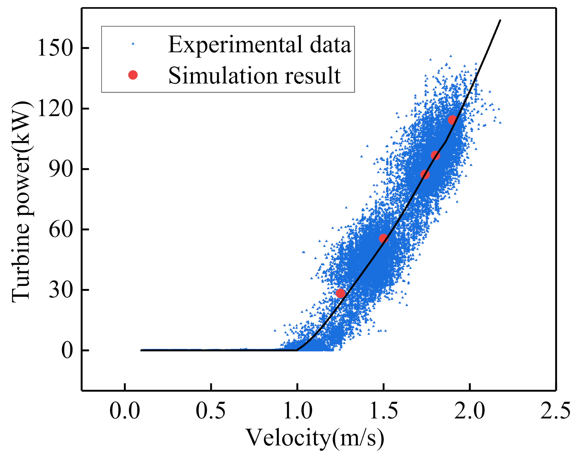
4.3. Effect of Sand on the Power of the 120 kW Tidal Current Turbine

When the particle diameter is large, the lift coefficient decreases with the increasing concentration. The airfoil lift and drag coefficients of 120 kW tidal current turbine were roughly estimated without considering the particle-to-particle interaction under a high particle concentration. Figure 21 shows the variation curves of lift and drag coefficients of Airfoil 28 with particle concentration when the particle diameter is 2500 μ m and the tidal current is 1.8 m/s. Based on Blade Element Momentum theory, the power of the 120 kW tidal current turbine was calculated under different particle concentrations, as shown in Table 7. When the particle concentration is 100 g/L, the rotor capture power is reduced by 21.4% at most compared to the particle-free case. The reduction in rotor capture power due to the particle concentration should be considered in the process of the tidal current turbine site selection and the blade design.
It has also been found that the airfoil lift coefficient increases when the particle diameter is small. Table 8 shows the power of the 120 kW tidal current turbine at different particle concentrations when the particle diameter is 20 μ m . When the particle concentration is 100 g/L, the rotor capture power is increased by 2.932% at most compared to the particle-free case, which is significant for the improvement of the tidal current turbine’s power.

5. Conclusions

In the paper, the CFD-DPM model was adopted to simulate the lift and the drag coefficients of the airfoil. The particle–fluid interaction was taken account in the CFD-DPM approach. The available experimental data for the120 kW tidal current turbine were used to validate the CFD-DPM model. Additionally, the lift and the drag coefficients of the airfoil under different particle properties were studied. Further, the 120 kW tidal current turbine power was calculated under different particle concentrations. According to the simulation results, the following conclusions can be drawn:
(1)
The CFD-DPM model accurately simulates the airfoil lift and drag coefficients.
(2)
When the particle diameter is small, the airfoil lift coefficient surpasses the particle-free lift coefficient. The lift coefficient increases as the particle concentration increases. When the particle diameter and the particle concentration are 20 μm and 100 g/L, respectively, the rotor capture power is increased by at most 2.932% compared to the particle-free case.
(3)
When the particle diameter is large, the airfoil lift coefficient is less than the non-particle lift coefficient. The lift coefficient decreases as the particle concentration increases. When the particle diameter and the particle concentration are 2500 μm and 100 g/L, respectively, the 120 kW tidal current turbine power is reduced by at most 21.4% compared to the particle-free case.
Conclusions (2) and (3) were roughly estimated using the CFD-DPM model under a large particle concentration. However, further investigation needs be conducted considering the particle-to-particle interaction under high particle concentrations.

Author Contributions

Y.G. (Yanjing Gao): Methodology, Formal analysis, Writing—Original Draft; H.L.: Writing—Review and Editing, Supervision, Funding acquisition; Y.L.: Writing—Review and Editing, Supervision, Funding acquisition; Y.G. (Yajing Gu): Conceptualization, Validation, Funding acquisition; Y.N.: Data Curation, Visualization. All authors have read and agreed to the published version of the manuscript.

Funding

This work was supported by National major research and development program (2018YFB1501900), Zhejiang Provincial major research and development program (2021C03182), Zhejiang Province Science and technology project (No. 2021R52040), and National Natural Science Foundation of China (No.51905472).

Institutional Review Board Statement

Not applicable.

Informed Consent Statement

Not applicable.

Data Availability Statement

Not applicable.

Conflicts of Interest

All authors declare that: (1) no support, financial or otherwise, has been received from any organization that may have an interest in the submitted work, and (2) there are no other relationships or activities that could appear to have influenced the submitted work.

Abbreviations

Variable SymbolsDefinitions
U p f n 
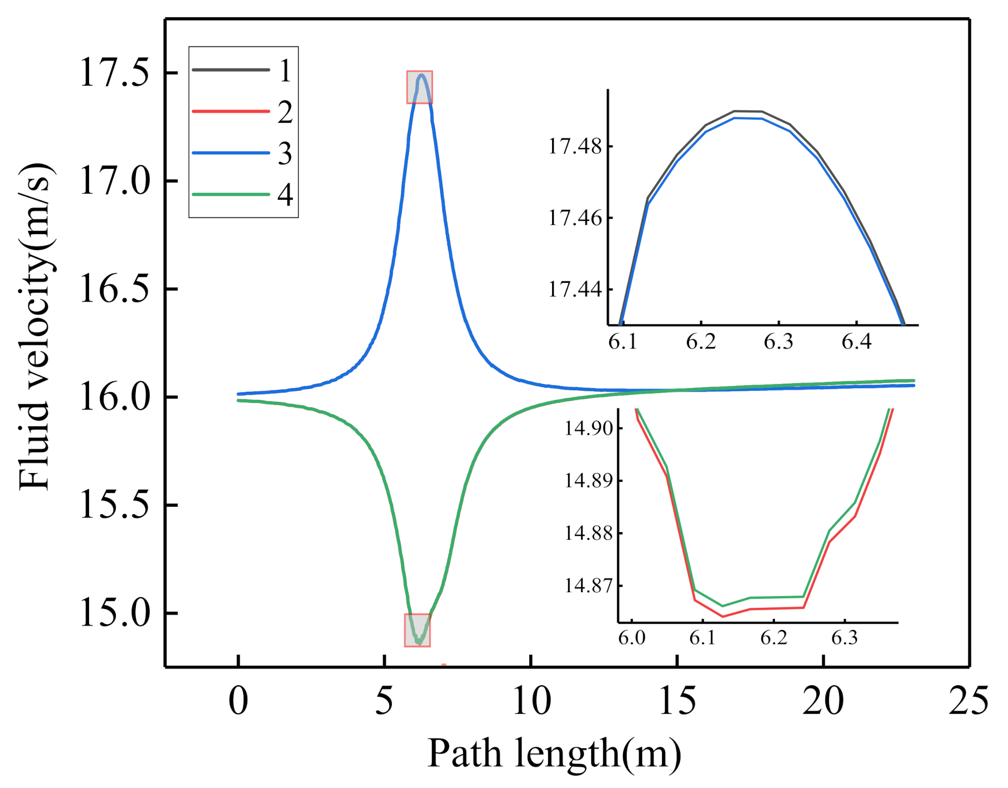
The difference between the particle velocity and the particle-free fluid velocity along the particle trajectory of the same Particle ID
U f p f n The difference between the fluid velocity and the particle-free fluid velocity along the particle trajectory of the same Particle ID
Time (in the Figure)Time beginning from the particle injection surface
Path length (in the Figure)Path length, defined as the path length of the particle trajectory, which is computed from the particle injection surface
CFDComputational Fluid Dynamics
BEMBlade Element Momentum
DEMDiscrete Element Method
DPMDiscrete Phase Model

References

  1. Myers, L.; Bahaj, A.S. Simulated electrical power potential harnessed by marine current turbine arrays in the Alderney Race. Renew. Energy 2005, 30, 1713–1731. [Google Scholar] [CrossRef]
  2. Li, D.; Wang, S.; Yuan, P. An overview of development of tidal current in China: Energy resource, conversion technology and opportunities. Renew. Sustain. Energy Rev. 2010, 14, 2896–2905. [Google Scholar] [CrossRef]
  3. Wang, S.; Yuan, P.; Li, D.; Jiao, Y. An overview of ocean renewable energy in China. Renew. Sustain. Energy Rev. 2011, 15, 91–111. [Google Scholar] [CrossRef]
  4. Wu, B.; Zhang, X.; Chen, J.; Xu, M.; Li, S.; Li, G. Design of high-efficient and universally applicable blades of tidal stream turbine. Energy 2013, 60, 187–194. [Google Scholar] [CrossRef]
  5. Gu, Y.J.; Yin, X.X.; Liu, H.W.; Li, W.; Lin, Y.G. Fuzzy terminal sliding mode control for extracting maximum marine current energy. Energy 2015, 90, 258–265. [Google Scholar] [CrossRef]
  6. Gupta, V.; Young, A.M. A one-dimensional model for tidal array design based on three-scale dynamics. J. Fluid. Mesh. 2017, 825, 651–676. [Google Scholar] [CrossRef] [Green Version]
  7. Attene, F.; Balduzzi, F.; Bianchini, A.; Campobasso, M.S. Using experimentally validated Navier-Stokes CFD to minimize tidal stream turbine power losses due to wake/turbine interactions. Sustainability 2020, 12, 8768. [Google Scholar] [CrossRef]
  8. Wang, X.K.; Shao, X.J.; Li, D.X. Fundamental River Mechanics; China Water & Power Press: Beijing, China, 2002; Available online: https://www.waterpub.com.cn (accessed on 8 April 2021).
  9. Yu, W.C.; Yue, H.Y. Position of runoff and sediment of Yangtze River in world rivers. J. Yangtze River Sci. Res. Inst. 2002, 6, 13–16. [Google Scholar]
  10. Zhang, R.J. River Sediment Dynamics, 2nd ed.; China Water & Power Press: Beijing, China, 1998; Available online: https://www.waterpub.com.cn (accessed on 8 April 2021).
  11. Ministry of Water Resource of the People’s Republic of China. China River Sediment Bulletin, China, Water & Power Press; Ministry of Water Resource of the People’s Republic of China: Beijing, China, 2019.
  12. Zuo, L.Q.; Lu, Y.J.; Ji, R.Y. Back silting law of the mouth bar channel in Southern Zhejiang muddy coastal estuaries: Case study of Aojiang Estuary. J. Basic Sci. Eng. 2014, 22, 88–105. [Google Scholar]
  13. Liu, L.Y. Suspended sediment simulation and numerical study of water purification scheme in turbid Zhoushan archipelago. In Proceedings of the OCEANS 2016, Shanghai, China, 10–13 April 2016. [Google Scholar]
  14. Fraenkel, P.L. Power from marine currents. Proc. Inst. Mech. Eng. Part A J. Power Energy 2002, 216, 1–14. [Google Scholar] [CrossRef]
  15. Ng, K.W.; Lam, W.H.; Ng, K.C. 2002–2012: 10 years of research progress in horizontal-axis marine current turbines. Energies 2013, 6, 1497–1526. [Google Scholar] [CrossRef] [Green Version]
  16. Batten, W.M.J.; Bahaj, A.S.; Molland, A.F. The prediction of the hydrodynamic performance of marine current turbines. Renew. Energy 2007, 33, 1085–1096. [Google Scholar] [CrossRef]
  17. Song, S.; Demirel, Y.K.; Atlar, M.; Shi, W.C. Prediction of the fouling penalty on the tidal turbine performance and development on its mitigation measures. Appl. Energy 2020, 276, 115498. [Google Scholar] [CrossRef]
  18. Walker, J.M.; Flack, K.A.; Lust, E.E. Experimental and numerical studies of blade roughness and fouling on marine current turbine performance. Renew. Energy 2014, 66, 257–267. [Google Scholar] [CrossRef]
  19. Gidaspow, D. Multiphase Flow and Fluidization: Continuum and Kinetic Theory Descriptions; Academic Press: Cambridge, MA, USA, 2012. [Google Scholar] [CrossRef]
  20. Guo, M.S.; Li, H.Z. Handbook of Fluidization; Chemical Industry Press Co., Ltd.: Beijing, China, 2008; Available online: https://www.cip.com.cn/ (accessed on 20 October 2021).
  21. Sun, L.; Ma, C.; Song, P.; Zhang, H. Quantitative computational fluid dynamic analyses of oil droplets deposition on vaneless diffusor walls of a centrifugal compressor. Energy Sci. Eng. 2020, 8, 910–921. [Google Scholar] [CrossRef]
  22. Cundall, P.A.; Strack, O.D.L. A discrete numerical model for granular assemblies. Geotechnique 1979, 29, 47–65. [Google Scholar] [CrossRef]
  23. Zhao, H.; Zhao, Y. CFD-DEM simulation of pneumatic conveying in a horizontal pipe. Powder Technol. 2020, 373, 58–72. [Google Scholar] [CrossRef]
  24. Wang, K.; Li, X.; Wang, Y.; He, R. Numerical investigation of the erosion behavior in elbows of petroleum pipelines. Powder Technol. 2017, 314, 490–499. [Google Scholar] [CrossRef]
  25. Zhou, M.M.; Wang, S.; Kuang, S.B.; Luo, K.; Fan, J.R. CFD-DEM modelling of hydraulic conveying of solid particles in a vertical pipe. Powder Technol. 2019, 354, 893–905. [Google Scholar] [CrossRef]
  26. Peng, W.S.; Cao, X.W. Numerical prediction of erosion distributions and solid particle trajectories in elbows for gas-solid flow. J. Nat. Gas Sci. Eng. 2016, 30, 455–470. [Google Scholar] [CrossRef]
  27. Peng, W.S.; Cao, X.W. Numerical simulation of solid particle erosion in pipe bends for liquid-solid flow. Powder Technol. 2016, 294, 266–279. [Google Scholar] [CrossRef]
  28. Morsi, S.A.; Alexander, A.J. An investigation of particle trajectories in two-phase flow systems. J. Fluid Mech. 1972, 55, 193–208. [Google Scholar] [CrossRef]
  29. Avi, U.; Avi, L. Flow characteristics of coarse particles in horizontal hydraulic conveying. Powder Technol. 2018, 58, 302–321. [Google Scholar]
  30. Saffman, P.G. The lift on a small sphere in a slow shear flow. J. Fluid. Mesh. 1965, 22, 385–400. [Google Scholar] [CrossRef] [Green Version]
  31. Haider, A.; Levenspiel, O. Drag coefficient and terminal velocity of spherical and nonspherical particles. Powder Technol. 1989, 58, 63–70. [Google Scholar] [CrossRef]
  32. Fatahian, H.; Salarian, H.; Nimvari, M.E.; Khaleghinia, J. Numerical simulation of the effect of rain on aerodynamic performance and aeroacoustic mechanism of an airfoil via a two-phase flow approach. SN Appl. Sci. 2020, 2, 867. [Google Scholar] [CrossRef]
  33. Zhou, Z.Y.; Kuang, S.B.; Chu, K.W.; Yu, A.B. Discrete particle simulation of particle–fluid flow: Model formulations and their applicability. J. Fluid Mech. 2010, 661, 482–510. [Google Scholar] [CrossRef]
  34. Karimi, S.; Shirazi, S.A.; McLaury, B.S. Predicting fine particle erosion utilizing computational fluid dynamics. Wear 2017, 376, 1130–1137. [Google Scholar] [CrossRef]
  35. Ahmadi, M.P.M.N. Particle Deposition in a Turbulent Channel Flow. In Fluids Engineering Division Summer Meeting; American Society of Mechanical Engineers: New York, NY, USA, 2013. [Google Scholar] [CrossRef]
  36. Menter, F.R. Two-equation eddy-viscosity turbulence models for engineering applications. J. AIAA 1994, 32, 1598–1605. [Google Scholar] [CrossRef] [Green Version]
  37. Li, W.; Zhou, H.B.; Liu, H.W.; Lin, Y.G.; Xu, Q.K. Review on the blade design technologies of tidal current turbine. Renew Sustain. Energy Rev. 2016, 63, 414–422. [Google Scholar] [CrossRef]
  38. Liu, H.W.; Zhou, H.B.; Lin, Y.G.; Li, W.; Gu, H.G. Design and test of 1/5th scale horizontal axis tidal current turbine. China Ocean Eng. 2016, 30, 407–420. [Google Scholar] [CrossRef]
  39. Burton, T.; Jenkins, N.; Sharpe, D.; Bossangi, E. Wind Energy Handbook; John Wiley & Sons, Ltd.: Chichester, UK, 2001. [Google Scholar]
  40. DNV GL. Tidal Bladed Theory Manual; Energy Headquarters: Arnhem, The Netherlands, 2012. [Google Scholar]
  41. Moriarty, P.J.; Hansen, A.C. AeroDyn Theory Manual; National Renewable Energy Lab: Golden, CO, USA, 2005.
  42. Gu, Y.J.; Liu, H.W.; Li, W.; Lin, Y.G.; Li, Y.J. Integrated design and implementation of 120-kW horizontal-axis tidal current energy conversion system. Ocean. Eng. 2018, 158, 338–349. [Google Scholar] [CrossRef]
  43. Yao, X.J.; Tian, D.; Song, J. Wind Generator’s Design and Manufacture; China Machine Press: Beijing, China, 2012; Available online: https://www.cmpedu.com (accessed on 20 October 2021).
  44. Ji, B.B.; Chen, J.P. ANSYS ICEM CFD Detailed Explanation of Grid Partition Technology Example; China Water & Power Press: Beijing, China, 2015. [Google Scholar]
  45. Ansys Fluent Inc. ANSYS FLUENT User Guide; Ansys Fluent Inc.: Canonsburg, PA, USA, 2018. [Google Scholar]
  46. Lewthwaite, M.T.; Amaechi, C.V. Numerical investigation of winglet aerodynamics and dimple effect of NACA 0017 airfoil for a freight aircraft. Inventions 2022, 7, 31. [Google Scholar] [CrossRef]
  47. Jia, W.; Yan, J. Pressure drop characteristics and minimum pressure drop velocity for pneumatic conveying of polyacrylamide in a horizontal pipe with bends at both ends. Powder Technol. 2020, 372, 192–203. [Google Scholar] [CrossRef]
  48. Farokhipour, A.; Mansoori, Z.; Rasoulian, M.A. Study of particle mass loading effects on sand erosion in a series of fittings. Powder Technol. 2020, 373, 118–141. [Google Scholar] [CrossRef]
  49. Li, D.S.; Wang, Y.; Guo, X.D.; Li, Y.R.; Li, R.N. Effects of particle shape on erosion characteristic and critical particle Stokes number of wind turbine airfoil. Trans. Chin. Soc. Agric. Eng. 2019, 35, 224–231. [Google Scholar]
  50. Li, Y.R.; Jin, J.J.; Han, W.; Li, D.S.; Zheng, L.K. Motion characteristics of diffuser diameter particles in flow field of S809 airfoil and effect of its aerodynamic performance. Acta Enegrgiae Sol. Sin. 2018, 39, 2923–2928. [Google Scholar]
  51. Li, R.N.; Zhao, Z.X.; Li, D.S.; Li, Y.R. Effects of wind sand on flow around airfoil of wind turbine and its aerodynamic performance. Trans. Chin. Soc. Agric. Eng. 2018, 34, 205–211. [Google Scholar]
Figure 1. Airfoil parameters: (a) geometric parameters and (b) hydrodynamic parameters.
Jmse 10 00515 g001aJmse 10 00515 g001b
Figure 2. Map of the location of the tidal current turbine.
Jmse 10 00515 g002
Figure 3. Photo of the sea trial in Zhoushan: (a) 120 kW tidal current turbine; (b) seawater with sediment.
Jmse 10 00515 g003
Figure 4. Blade profile of the 120 kW tidal current turbine: (a) blade profile; (b) detailed airfoil element section.
Jmse 10 00515 g004
Figure 5. Calculation domain and boundary conditions.
Jmse 10 00515 g005
Figure 7. Comparison of the simulated lift and drag coefficients with the experimental data.
Jmse 10 00515 g007
Figure 8. Erosion diagram of the 120 kW tidal current turbine: (a) the actual erosion diagram under real sea conditions; (b) the simulated erosion cloud diagram at 1.8 m/s (blade contains 30 airfoil elements, the airfoil element at the tip is named “airfoil 30”, and the others are named in sequence. Additionally, Er represents the average erosion rate).
Jmse 10 00515 g008
Figure 9. Comparison of the maximum erosion location of the simulation and the experiment.
Jmse 10 00515 g009
Figure 10. Comparison of the simulated turbine power with the experimental data at different flow velocities.
Jmse 10 00515 g010
Figure 11. The airfoil lift coefficient with the particle diameter under different particle concentrations.
Jmse 10 00515 g011
Figure 12. The particle trajectories and the fluid streamlines when the particle diameter is 20 μ m : (a) the particle trajectories; (b) the fluid streamlines.
Jmse 10 00515 g012
Figure 13. The particle velocity and the fluid velocity along the trajectory of Particle ID = 5 (particle diameter = 20 μ m ).
Jmse 10 00515 g013
Figure 14. The particle velocity and the particle-free fluid velocity along the trajectory of Particle ID = 5 (particle diameter = 2500 μ m ).
Jmse 10 00515 g014
Figure 15. The effect of particle concentration on the airfoil lift coefficient.
Jmse 10 00515 g015
Figure 16. The particle velocities and the particle-free fluid velocities along the trajectory of particle ID = 5 under different particle concentrations.
Jmse 10 00515 g016
Figure 17. The particle trajectories under different particle concentrations: (a) 0.5 g/L; (b) 1 g/L; (c) 1.5 g/L; (d) 2 g/L.
Jmse 10 00515 g017
Figure 18. The airfoil drag coefficient with the particle diameter under different particle concentrations.
Jmse 10 00515 g018
Figure 19. The velocities of fluid along the trajectories of Particle ID = 23,000 and Particle ID = 45,000 (1: Particle ID = 45,000 without particles; 2: Particle ID = 23,000 without particles; 3: Particle ID = 45,000 (particle diameter = 2500 μ m ); 4: Particle ID = 23,000 (particle diameter = 2500 μ m )).
Jmse 10 00515 g019
Figure 20. The effect of particle concentration on the airfoil lift coefficient.
Jmse 10 00515 g020
Figure 21. The variation curves of lift and drag coefficients of airfoil 28 with particle concentration when the particle diameter is 2500 μ m : (a) lift coefficient; (b) drag coefficient.
Jmse 10 00515 g021
Table 1. 120 kW tidal current turbine design parameters.
Design ParametersValue
Rated tidal current velocity2 m/s
Rated rotor rotating velocity20 r/min
Blade number3
Rotor radius5 m
Hub radius0.6 m
Optimal tip speed ratio6
Table 2. 120 kW tidal current turbine blade geometrical parameter distributions along the blade.
Distance Along Pitch Axis (m)Chord (m)Twist (°)Thickness (%)
00.46022.5100
0.40.62222.4568.1
0.80.87218.2736.1
1.250.71812.6231.1
1.70.5779.0327.6
2.20.4696.3725
2.80.3914.1922.2
3.40.3262.6121
3.80.2681.6421
4.20.2410.5421
4.40.152016
Table 3. Particle size distribution detail in Zhoushan.
Minimum DiameterMaximum DiameterMedian DiameterMean Diameter
5 × 10 7 m 2 . 84 × 10 4 m 4 . 2 × 10 5 m 1 . 2 × 10 5 m
Table 4. Simulation parameters employed in the current simulations.
Liquid Property
Density, (Kg/m3)1040
Temperature, (°C)25
Viscosity, (Kg/(m s))0.00115
Solid Property
Materialsand
Density, (Kg/m3)2650
Table 5. Operating conditions of the simulation cases.
Operating
Parameters
dP  ( μ m ) CP (g/L)α (°)c (m)U (m/s)
Effect of particle properties20∼30000.5~26116
Table 7. The power of the 120 kW tidal current turbine at different particle concentrations when the particle diameter is 2500 μ m .
Particle Concentration/(kg/m3)Power/(W)(P0 *-P)/P0 *
096,7100
296,2060.521%
595,4321.32%
2092,2774.58%
4087,6749.34%
8080,87417.5%
10076,02021.4%
* P0: rotor capture power without particles.
Table 8. The power of the 120 kW tidal current turbine at different particle concentrations when the particle diameter is 20 μ m .
Particle Concentration/(kg/m3)Power/(W)(P0 *-P)/P0 *
096,7100
296,7640.0558%
596,8350.129%
2097,1760.482%
4097,4110.725%
8098,3971.744%
10099,5462.932%
* P0: rotor capture power without particles.
Publisher’s Note: MDPI stays neutral with regard to jurisdictional claims in published maps and institutional affiliations.

