Flow Characteristics of Oblique Submerged Impinging Jet at Various Impinging Heights

Abstract

To study the influence of impinging height H/D on the flow field characteristics of oblique submerged impinging jets, the numerical calculation of an oblique submerged impinging jet was carried out based on Wray–Agarwal (W–A) turbulence model. The jet flow field structure and pressure distribution under various impinging heights (1 ≤ H/D ≤ 8) when the impinging angle was θ = 45° were analyzed. The results show that with the increase in the impinging height, the diffusion degree of the jet gradually increased and the velocity decreased when the jet reached the impingement region, and the distance between the stagnation point (SP) and the geometric center (GC) gradually increased, the flow angle φ along the jet centerline remained constant in the free-jet region and rapidly decreased in the impingement region. The impingement plate pressure distribution at various heights was similar, and the impinging pressure concentration on the upstream side of the maximum pressure point was higher.

1. Introduction

Impinging jet refers to the impinging flow of free jets on solid or liquid surfaces. It is widely used in daily life and has been widely used in the field of engineering technology, such as micro-spray irrigation in water-saving irrigation, cooling and heating in industrial manufacturing, high-pressure water jet cutting, and other applications. With the progress of experimental technology and the development of computational fluid dynamics, many scholars have explored the internal flow field and heat transfer characteristics of impinging jet from the nozzle shape, impinging angle, number of jets, jet velocity and other aspects, and obtained the entrainment, mixing and impact characteristics of the internal fluid of impinging jest, which enriches the jet theory and has been applied in practical problems.

As a widely existing flow form, impinging jet has important engineering application significance. Many studies have focused on vertical impinging jets. Cooper et al. [1] measured the average velocity components of the vertical circular impinging jet at various impinging heights by hot-wire anemometer, and the experimental results are widely used in the development and verification of turbulence models. Ashforthfrost et al. [2] used a laser-Doppler anemometer to study the influence of nozzle geometry and semi-confined cases on the potential core of vertical jets, and found that the potential core of fully developed jet is 7% longer. Alekseenko et al. [3] studied the flow structure of turbulent impinging jets under different swirl rate by using particle image velocity measurement and found that the swirl impinging jet studied had larger diffusion rate and faster absolute velocity attenuation. Hammad et al. [4] analyzed the flow structure of the pipe outlet, impingement region, and wall-jet region in vertical impact at different heights by particle image velocimetry, and found that the correlation of the 1/6th power law provides a good approximation for the fully developed turbulence profile. Xu et al. [5] studied the sensitivity of vertical impinging jets to Reynolds number, surface roughness, and inlet conditions, and found that inlet turbulence mainly affects the free-jet region. Fitzgerald et al. [6] studied a confined vertical submerged impinging jet with perfluorinated dielectric liquid (FC-77) as the medium by laser-Doppler velocimeter. The results showed the effects of the distance between the nozzle and the plate and the nozzle diameter on the peak turbulence levels. Lai et al. [7] studied impulsively started impinging jets by using fluorescent dye technology and found that the velocity of the jet-front varied with the square root of time. Pieris et al. [8] used time-resolved two-component particle image technology to analyze the flow development of impinging jets at various impinging heights and Reynolds numbers, and quantitatively described the vortex dynamics characteristics under various working conditions. Hanson et al. [9] obtained the pressure and shear stress distribution of a submerged vertical impinging jet at the planar boundary and established an empirical relationship to describe the shear stress distribution at the boundary of the impingement region. With the development of computational fluid dynamics and the improvement of computational performance, the computational accuracy of numerical simulation is continuously improved and applied more widely [10,11,12]. Combined with experimental applications in practical engineering [13,14,15], the research ability is enhanced, and the complex mechanism of impinging jets is gradually explored. Wang et al. [16] used the large eddy simulation (LES) method to numerically simulate the unsteady flow in an impinging jet and used the Lagrangian scheme for particle tracking to simulate the unsteady erosion of the target surface. Sabato et al. [17] studied the influence of several configurations of submerged impinging jet on the cooling of power electronic equipment through numerical simulation and derived a reasonable value range for nozzle diameter and nozzle number. Zerrout et al. [18] carried out a numerical simulation of a multi-jet system under various impinging heights, velocity, and other conditions, and, compared with the experimental results, it was found that the calculation results of the two-equation transport model (k-ε) were more accurate. Abdel et al. [19] conducted a numerical study on the three-dimensional turbulent flow field of jet impinging on a rotating disk and presented the influence of nozzle to disk distance and Reynolds number on the flow characteristics and pressure characteristics. So et al. [20] adopted the large eddy simulation method to analyze the flow structure of impinging jets under different nozzle widths and nozzle-to-plate distances. By analyzing the flow field, the flow characteristics of impinging jets were classified according to the dimensionless distance. However, compared to vertical impinging jets, oblique impinging jets have received relatively less attention; most are water jets in the air, and there are fewer studies on submerged oblique impinging jets. Wang et al. [21] analyzed the flow characteristics of impinging jets under various impinging angles and Reynolds numbers through particle image velocity and pressure measurement and found that the jet is more dependent on the impinging angle and relatively independent of the Reynolds number. Mishra et al. [22] used particle image velocity measurement to analyze the flow characteristics of oblique submerged jets with impinging angles of 45° and 26° and an impinging height of 1D~6D (D is the nozzle diameter). They found that there is a critical impinging angle, below which there is no flow of the jet in the uphill region. Jalil et al. [23] studied the flow characteristics of impinging jets under different nozzle diameters and impinging angles and found that when the impinging angle is less than 45°, the deflected jet rarely flows backward, and that the estimated value may increase by 5~10% when the impinging angle is larger. Jiao et al. [24] used a new one-equation turbulence model to analyze the flow field characteristics and impinging pressure variation of oblique submerged jets at different times, and found that the impinging plate pressure was affected by Reynolds number, but that the distribution trend remained unchanged.

In summary, previous studies on oblique submerged impinging jets are relatively few. As a complex flow, they have a practical engineering application background. Compared with the previous research on oblique submerged impinging jet, this paper innovatively adopts the Wray–Agarwal (W–A) turbulence model, studies the influence of oblique jet at various Reynolds numbers, and gives the variation law of oblique jet impact pressure at different heights. Firstly, when the Reynolds number (Re) was 35,100, we studied the influence of impinging height on the flow field in the free-jet region and near-wall region of 45° oblique submerged impinging jet. In addition, when calculating the impinging pressure at various heights, we analyzed the influence of different Reynolds number conditions (11,700 ≤ Re ≤ 35,100).

2. Calculation Model and Numerical Method

2.1. Geometric Model and Boundary Conditions

The submerged impinging jet model is shown in Figure 1: The fluid is ejected from a circular nozzle with diameter D, length 50 D, and angle θ = 45° to the horizontal plane, obliquely impinging on the bottom of the tank. The front and rear sides of the sink are fixed wall surfaces, the left and right sides are outlets, and the top surface is a free surface. The length of the tank L_w is 55D, the width W_w is 7D, and the height Hw is 12D. Two coordinate systems of ro₁l and o₂xyz are established. The origin o₁ in the ro₁l coordinate system is at the center of the jet pipe outlet. The r-axis is the radial direction of the jet pipe, and the l-axis is the axial direction of the jet pipe, that is, the jet impingement direction. The origin o₂ in the o₂xyz coordinate system is located at the intersection of the extension line of the center line of the jet pipe and the impingement plane, that is, the geometric center (GC). The axis x and axis z correspond to the parallel and vertical directions of the impingement plane, respectively, and the axis y is perpendicular to the plane. As shown in Figure 1b, the flow angle φ of the jet can represent the flow direction of each point in the mid-section (o₂xz section) of the jet, and its size is defined as φ = arctan (−V_z/V_x). The jet velocity at the outlet of the pipe is set as V, the average velocity at the outlet V_b = 4Q/πD², and the maximum velocity is the jet center velocity V_max.

The calculation area was divided into structured grids by ICEM software. As shown in Figure 2a, the velocity inlet condition was adopted. According to the velocity measured in the previous experiment, the three working conditions were set as 0.585 m/s, 1.17 m/s, and 1.76 m/s, respectively, and the corresponding Reynolds numbers were Re = 11,700, Re = 23,400, and Re = 35,100, respectively. The rigid-lid hypothesis method was adopted on the top free surface and set as the symmetry boundary conditions. Since the length of the experimental water tank was much greater than that of the simulated water tank, the left and right sides were set as pressure outlets with a gauge pressure of 0 Pa, and the rest were set as non-slip fixed wall. The most suitable grid size was determined by analyzing the independence of the number of grids. Five schemes were obtained by determining different grid sizes, and the number of grids was 2.65 × 10⁶, 3.21 × 10⁶, 3.73 × 10⁶, 4.26 × 10⁶, 4.80 × 10⁶. As shown in Figure 2b, with the increase in the number of grids, the numerical simulation results gradually approached those of the experimental results, and the number of grids was finally determined to be 4.26 million.

2.2. Turbulence Model Selection

The Wray–Agarwal (W–A) turbulence model is a one-equation model developed based on the k-ω model [25,26,27]. Wang et al. [28] used Wray–Agarwal, Standard k-ε, Renormalization Group k-ε (RNG k-ε), Realizable k-ε, Standard k-ω and Shear Stress Transfer k-ω (SST k-ω) turbulence models for numerical calculations under the parameters of impinging angle θ = 45° and impinging height H/D = 3. Combined with Particle Image Velocimetry (PIV) experimental results [21], the difference between V/V_max of circular jet outlet velocity and empirical formula V/V_max = (1 − 2 r/D)^1/n reflecting fully developed jet outlet velocity was compared. When n = 7, the velocity profiles were approximately consistent with those of the fully developed circular jet. Figure 3 shows that the calculation results based on W–A model were closest to the PIV results and the empirical formula.

The W–A turbulence model not only adopts the ω equation with the cross-diffusion term, but also retains the link to the k-ε model, improving the accuracy of predicting equilibrium flow and the ability to explain non-equilibrium flow.

The eddy viscosity equation is as follows:

$${\mu }_{\tau }=f_{\mu }\rho R$$

(1)

$$R=\frac{k}{\omega }$$

(2)

The transport equation of the variable R in W–A model is as follows:

$$\frac{\partial \rho R}{\partial t}+\frac{\partial \rho u_{j}R}{\partial x_j}=\frac{\partial }{\partial x_j}\left[\left({\sigma }_R{\mu }_{\tau }+\mu \right)\frac{\partial R}{\partial x_j}\right]+\rho C_{1}RS+\rho f_1{C}_{2k\omega }\frac{R}{S}\frac{\partial R}{\partial x_j}\frac{\partial S}{\partial x_j}-\left(1-f_1\right)\rho C_{2k\epsilon }\left(\frac{R\frac{\partial S}{\partial x_j}}{S}\right)$$

(3)

The constants C₁, C_2kω, C_2kε, and σ_R are determined from empirical data and the wall constraint law:

$$\begin{gathered} C_{1k\omega }=0.0829,C_{1k\epsilon }=0.1127,C_1=f_1\left(C_{1k\omega }-C_{1k\epsilon }\right)+C_{1k\epsilon }, \\ {\sigma }_{k\omega }=0.72,{\sigma }_{k\epsilon }=1.0,{\sigma }_R=f_1\left({\sigma }_{k\omega }-{\sigma }_{k\epsilon }\right)+{\sigma }_{k\epsilon }, \\ {C}_{2k\omega }=\frac{C_{1k\omega }}{{\kappa }^2}+{\sigma }_{k\omega },C_{2k\epsilon }=\frac{C_{1k\epsilon }}{{\kappa }^2}+{\sigma }_{k\epsilon },\kappa =0.41 \end{gathered}$$

(4)

S is the mean strain, given as:

$$S=\sqrt{2S_{ij}{S}_{ij}}$$

(5)

The wall blocking effect is accounted for by the damping function f_μ:

$$f_{\mu }=\frac{{\chi }^3}{{\chi }^3+C_W^3}, \chi =\frac{R}{v}$$

(6)

The existence of the two terms C_2kω and C_2kε makes the W–A turbulence model behave as a one-equation k-ω model or a one-equation k-ε model, and f₁ is the switching function, defined as:

$$f_1=tanh({arg}_1^4)$$

(7)

$${arg}_1=min\left[max(\frac{\sqrt{R}}{0.164d\sqrt{S}},\frac{150\nu }{d^{2}S}),\frac{2R{S}^2}{d^{2}CrossDiff}\right]$$

(8)

$$CrossDiff=S\frac{\partial R}{\partial x_j}\frac{\partial S}{\partial x_j}+R\frac{\partial S}{\partial x_j}\frac{\partial S}{\partial x_j}$$

(9)

where d is the minimum distance to the nearest wall.

3. Results and Discussion

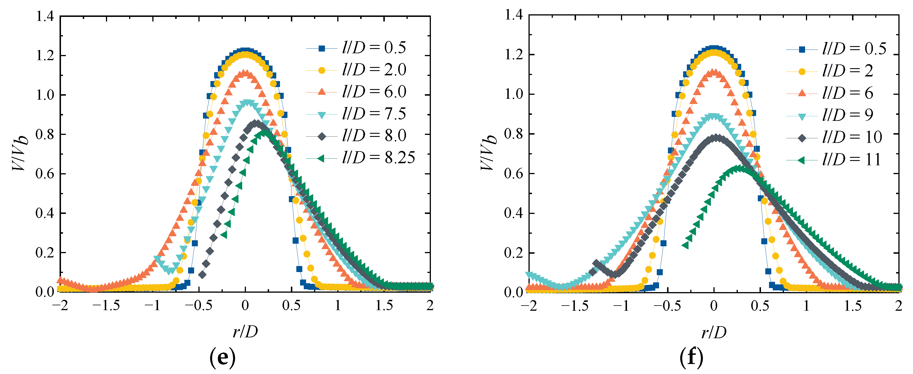
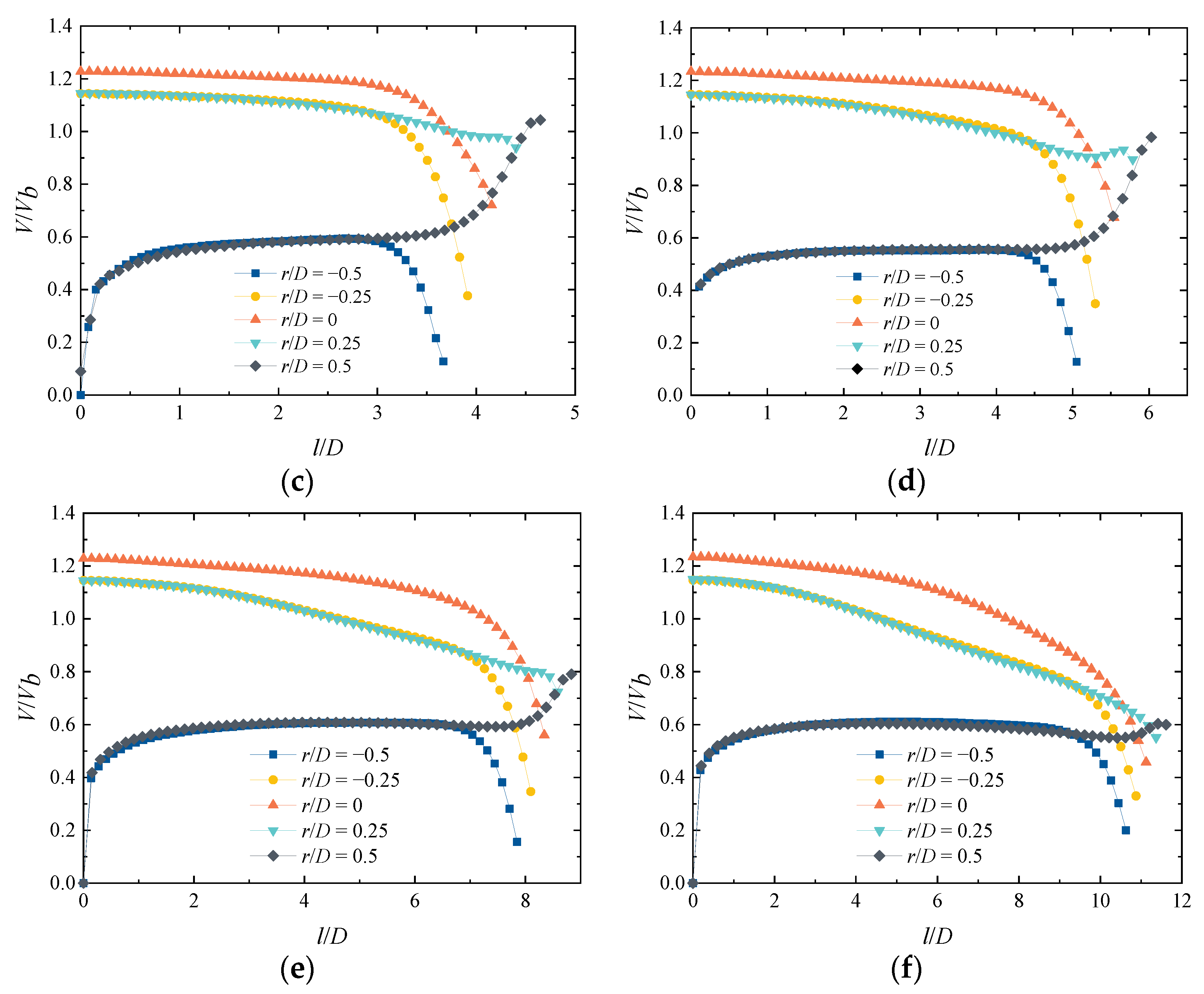
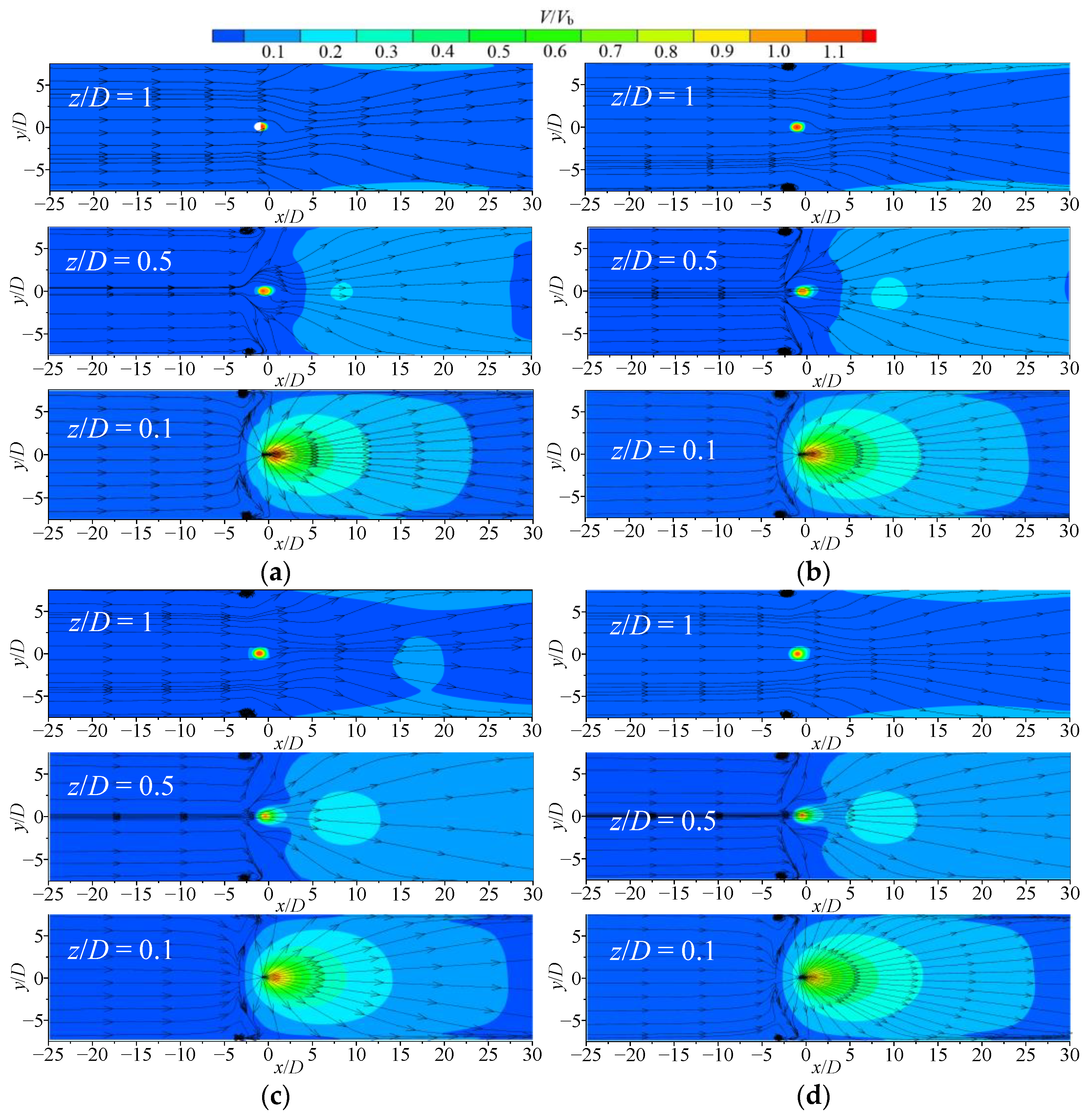
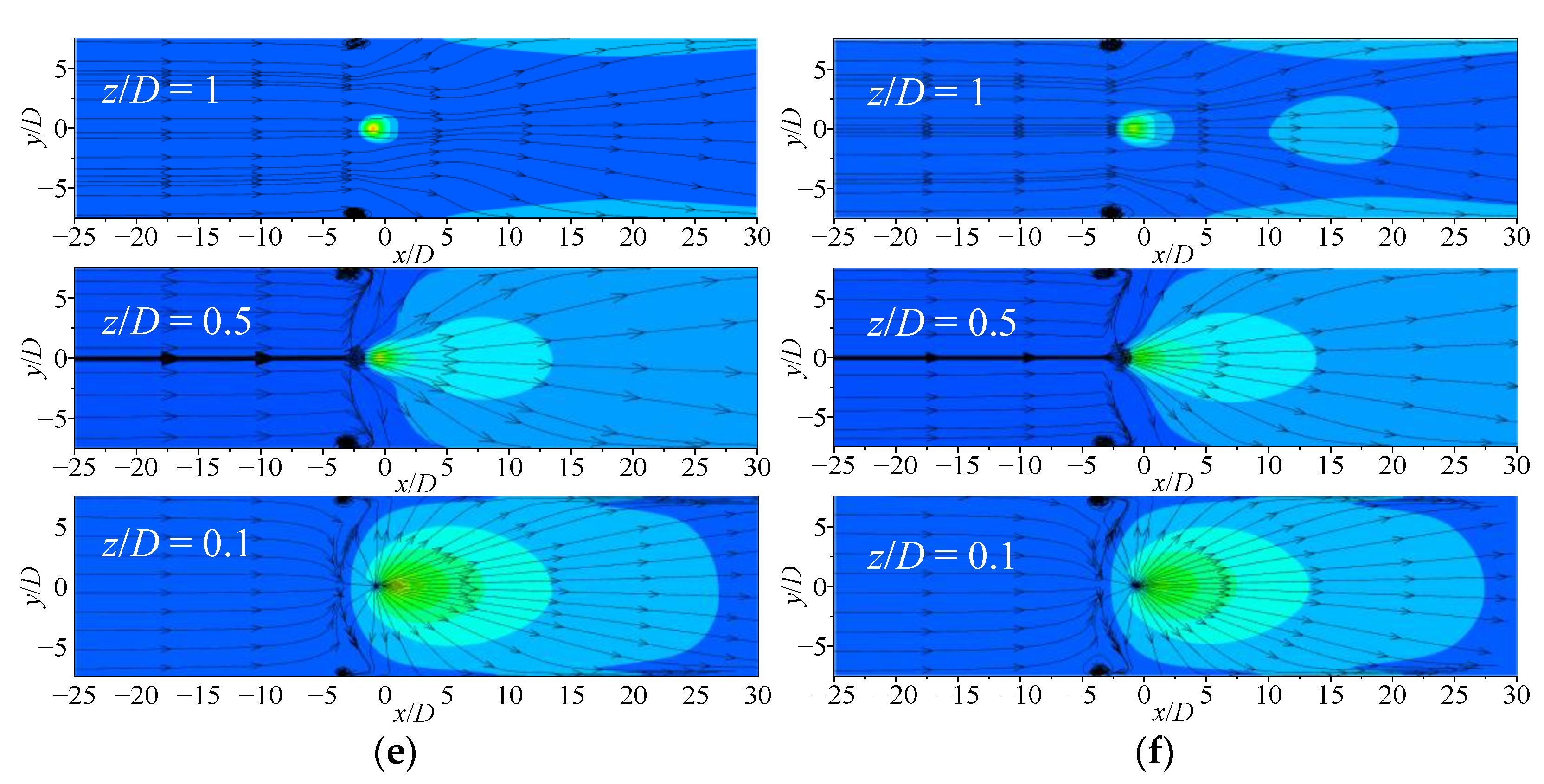
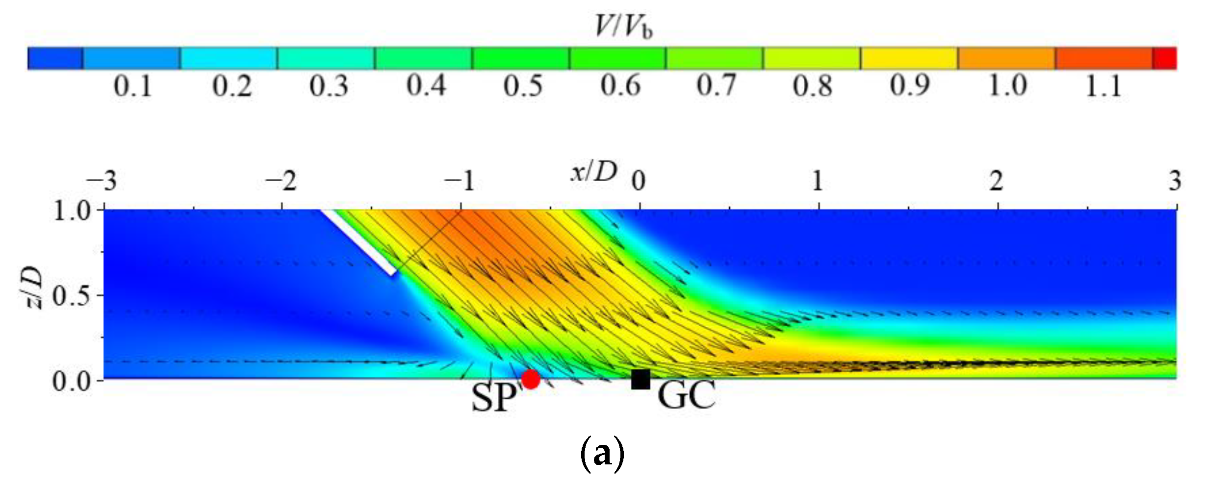
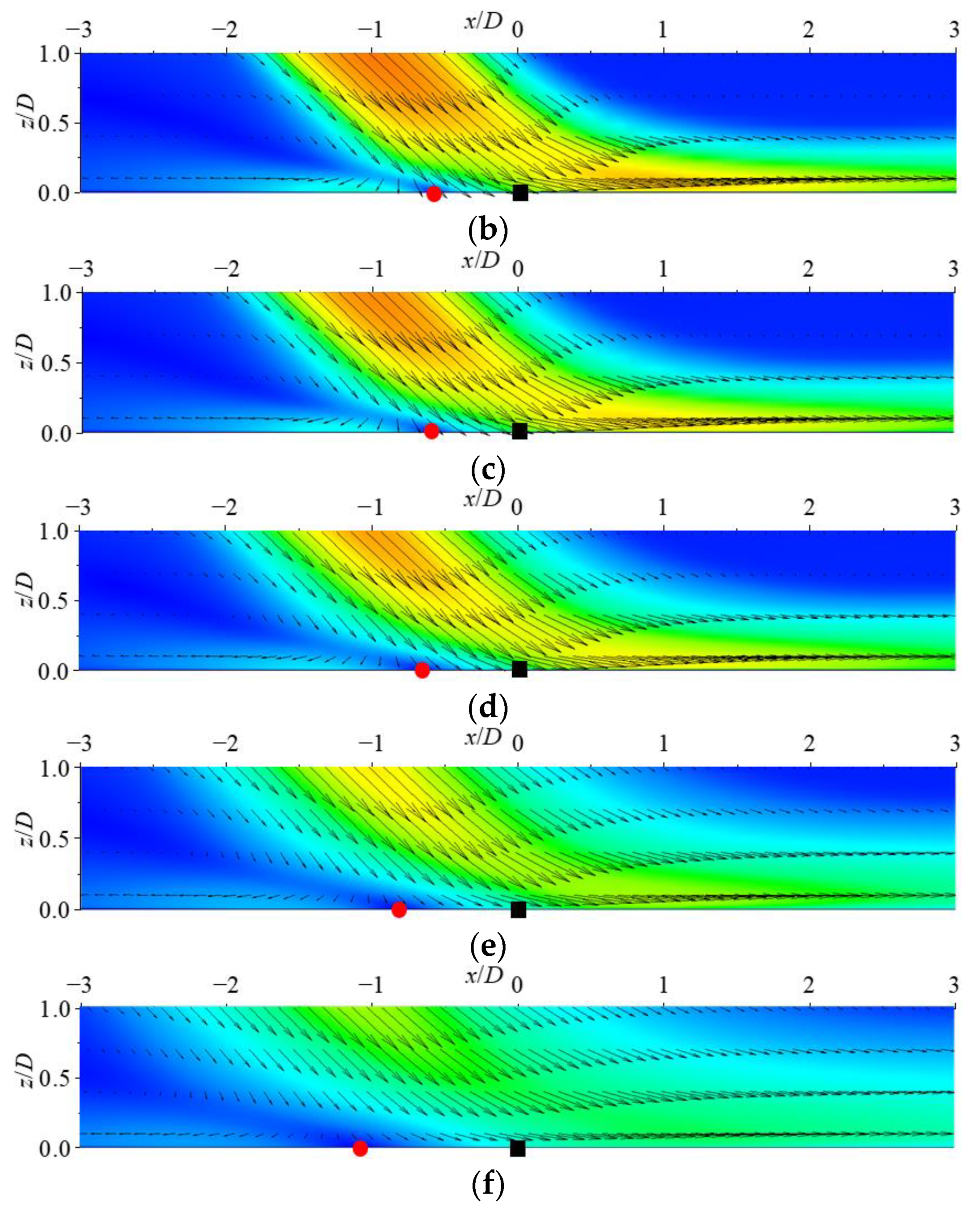
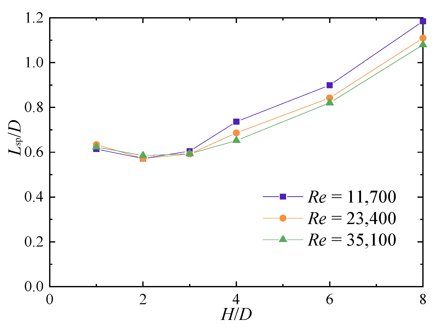
3.1. Analysis of Submerged Jet Flow Field under Various Impinging Heights

The streamline of the submerged jet at various impinging heights is shown in Figure 4 (Re = 35,100). When the impinging height is low, the flow direction of the jet fluid deflects when it impacts on the plane. Most of the fluid flows in the downstream direction (+x direction), and a small amount of fluid flows in the upstream direction (−x direction); the vortex is generated near the impact origin in the upstream direction. After the vortex moves horizontally to the two sides of the wall and collides, it moves in the downstream direction, and the vortex range gradually increases. With the increase in the impinging height, the intensity of the vortex gradually weakens.

Figure 5 shows the velocity cloud chart and streamline (Re = 35,100) of the middle section (y/D = 0) V/V_b of the jet at various impinging heights. When the impinging height increases, the jet flow distance between the nozzle and impact plane increases, and the jet diffusion range increases gradually. When H/D ≤ 4, the jet fluid has a greater axial velocity when it reaches the impingement region; when H/D ≥ 6, the axial velocity gradually decreases when it reaches the impingement region. Vortex (C₁~C₆) is generated near the impact origin in the jet upstream direction (−x direction), and the vortex center location is consistent, and is almost unaffected by the impinging height.

The V/V_b velocity cloud chart and streamline (Re = 35,100) of jet cross sections (z/D = 1, 0.5, 0.1) at different impinging heights are shown in Figure 6. The velocity cloud chart and streamline of the jet have good symmetry. In the z/D = 1 section, when H/D ≥ 2, small-scale vortices appear near the two side walls (x/D = −2.5), and the ambient fluid in the upstream flow direction of the jet is sucked into the vortex. In the z/D = 0.5 section, it is found that when the impinging height H/D ≥ 3, the jet velocity cloud chart of the impingement region and the wall-jet region is connected, indicating that the thickness of the wall-jet near the impingement region increases with the increase in the impinging height. The section with z/D = 0.1 is closest to the impact plate. It was found that the increase of impinging height leads to the gradual decrease of the maximum velocity in the impingement region and the influence range of the jet velocity. When H/D ≥ 3, the velocity distribution range remains unchanged. The results show that with the increase in impinging height, the jet velocity in the impingement region decreases gradually at the same position, and the jet fluid thickness increases from the impingement region to the wall-jet region.

Figure 7 shows the axial velocity V/V_b, horizontal velocity |V_x|/V_b, and vertical velocity |V_z|/V_b (H/D = 1, 8) of the jet at different Reynolds numbers (Re = 11,700~35,100). When H/D = 1, V/V_b remains unchanged in the range of 0 ≤ l/D ≤ 0.2; when l/D ≥ 0.2, V/V_b decreases with the increase in l/D, |V_z|/V_b decreases rapidly from 0.9 to 0, and |V_x|/V_b remains unchanged after slightly decreasing. At the same axial location, l/D, the values of V/V_b, |V_x|/V_b, and |V_z|/V_b at low Reynolds numbers are slightly higher than those of higher Reynolds numbers, but the velocity profiles have good similarity. When H/D = 8, V/V_b, |V_x|/V_b and |V_z|/V_b decrease gradually with the increase in l/D in the potential core region and transition region (0 ≤ l/D ≤ 10.5), and the decay rates of |V_x|/V_b and |V_z|/V_b are fundamentally the same; in the impingement region (l/D ≥ 10.5), the decay rates of |V_x|/V_b and |V_z|/V_b increase. It can be seen from Figure 7 that an increase in impinging height leads to an increase in jet flow distance and a decrease in jet velocity when it reaches the impingement region. The velocity profiles are similar under different levels of Re, which indicates that Reynolds number has little effect on velocity profiles.

The radial profiles of jet axial velocity V/V_b at different impinging heights are shown in Figure 8 (Re = 35,100). When the impinging height H/D = 1, the velocity profiles are obviously asymmetrical under the influence of the impact wall. The maximum value of V/V_b deviated from the axis, and with the increase in l/D, it decreases rapidly at first and then remains almost constant. When H/D = 2, the jet velocity profiles show good symmetry in the range of 0 ≤ l/D ≤ 3.0, −0.5 < r/D ≤ 0.5; in the range of −2.0 < r/D ≤ −0.5, the jet flows in the upstream direction, and the V/V_b decreases first and then increases. When l/D ≥ 2.5, the location where the maximum value of V/V_b is deflected toward +r direction, and the maximum value of V/V_b is approximately equal to 1. When H/D = 3, in the range of 0 ≤ l/D ≤ 1.5, the velocity profiles show good symmetry, and the maximum value of V/V_b is basically unchanged; when l/D > 3, the maximum value of V/V_b decreases with the increase of l/D. When H/D = 4, the range of the jet potential core region increases, but the maximum value of V/V_b near the wall decreases. This is caused by the increase in jet flow distance and the large attenuation of jet velocity in the transition region. When H/D = 6, the jet flow distance increases, the transition region range becomes larger, and the velocity entering the impingement region decreases. The maximum value of V/V_b near the wall is about 0.8. When H/D = 8, in the free-jet region, the impingement plane has little effect on the jet, and the jet is in a good axisymmetric shape; the maximum value of V/V_b near the wall decreases to about 0.6. It can be seen from the figure that at low impinging height (H/D ≤ 3), the velocity attenuation of the jet center is small, and the maximum value of V/V_b near the wall remains near 1. When the impinging height increases, the jet flow distance increases, the jet diffusion degree increases, and the maximum value of V/V_b near the wall decreases gradually. When H/D = 8, the maximum value of V/V_b near the wall is about 0.6, and nearly half of the initial velocity is lost, indicating that the impinging height has a great influence on the jet velocity.

Figure 9 shows the axial profile development of velocity V/V_b at different radial locations (r/D = 0, ±0.25, and ±0.5) under various impinging heights (Re = 35,100). Within the calculated height range, the flow distance of the jet between the nozzle and the impingement plane is l/D = h/(D × sinθ) ≈ 1.4~11.3, and it is generally considered that the length of the jet potential core region is 4~6 D. Therefore, when H/D = 1~3, there is only the potential core region in the free-jet region, and the velocity V/V_b remains fundamentally unchanged at r/D = 0 and ±0.25. When H/D ≥ 4, there is a transition region in the free-jet region, and the velocity V/V_b at r/D = 0 and ±0.25 first remains unchanged and then decreases with the increase in l/D; at r/D = ±0.5, the velocity V/V_b increases gradually and then tends to be stable, and the momentum is the main factor driving the jet flow. In the impingement region, the velocity V/V_b decreases gradually at r/D = 0, ±0.25 and −0.5, and the velocity V/V_b decreases slightly at r/D = 0.25 due to the jet deflecting in the downstream direction in the impingement region, and the increase in |Vx| is lower than the decrease in |Vz| in the impingement region; at r/D = 0.5, the velocity V/V_b gradually increases, and the increment decreases with the increase in impinging height. When H/D = 1, the velocity V/V_b increases by about 0.55, while when H/D = 8, the velocity is almost unchanged.

Figure 10 shows the variation law of flow angle φ (Re = 35,100) in each radial direction (r/D = 0, ±0.25 and ±0.5) of jet under various impinging heights. In the free-jet region, the flow angle φ is always close to the impinging angle θ. At this time, the impingement plane has little influence on the flow, and the changes in |V_x| and |V_z| are basically the same. In the impingement region, the values of φ decay linearly with l/D at r/D = 0, ±0.25, and 0.5, and the decay rates are different at various radial locations. The flow angle φ increases gradually at r/D = −0.5. When H/D = 1, the maximum value of φ is greater than 90°, and there is a countercurrent flow; when H/D ≥ 2, the flow angle φ is less than 90°, indicating that the flow deflects in the downstream direction.

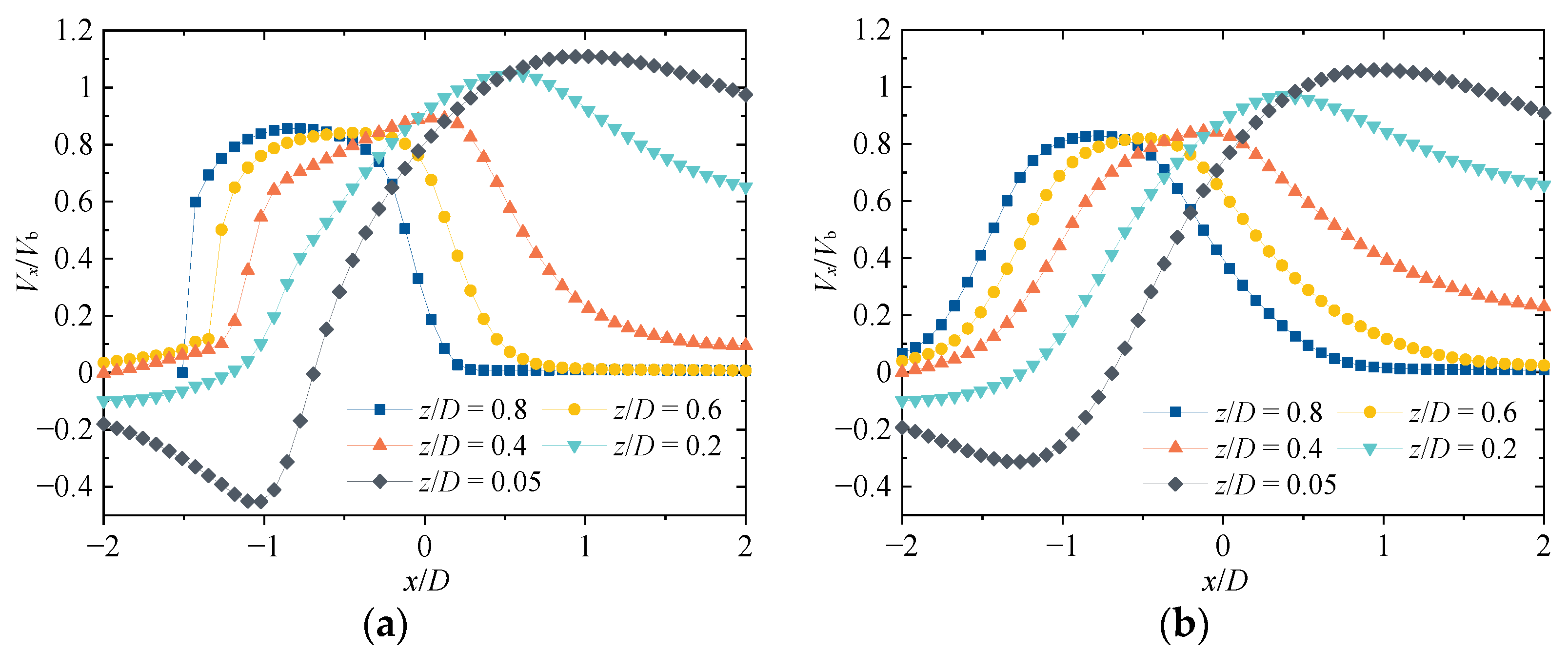
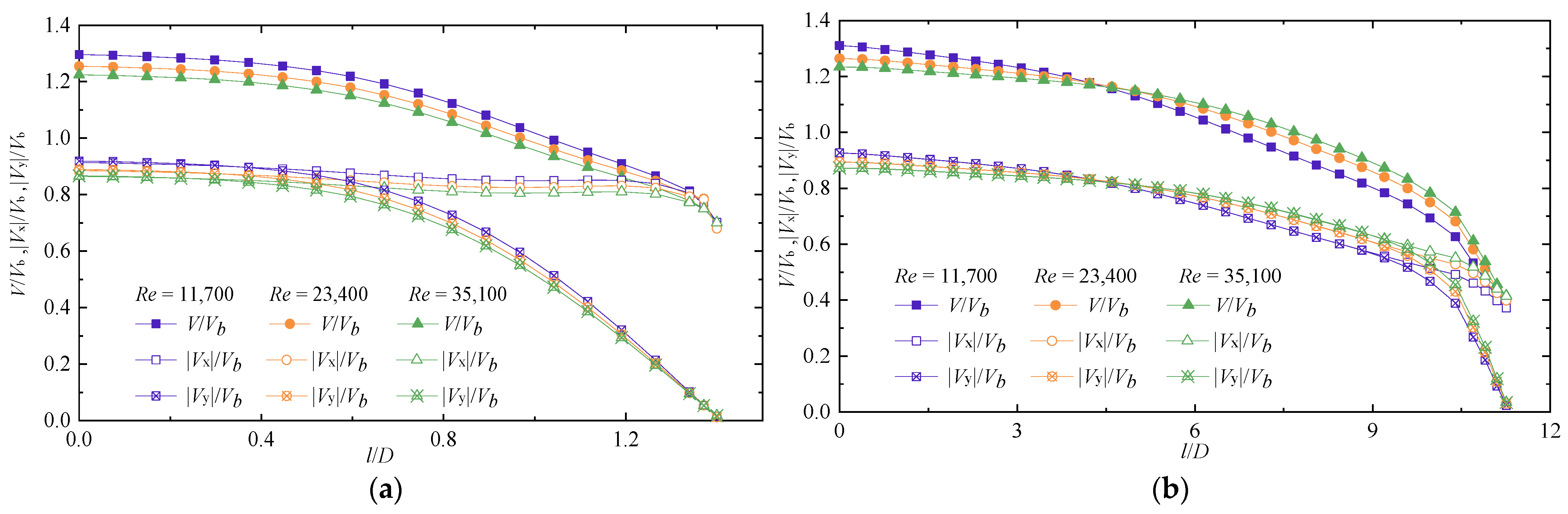
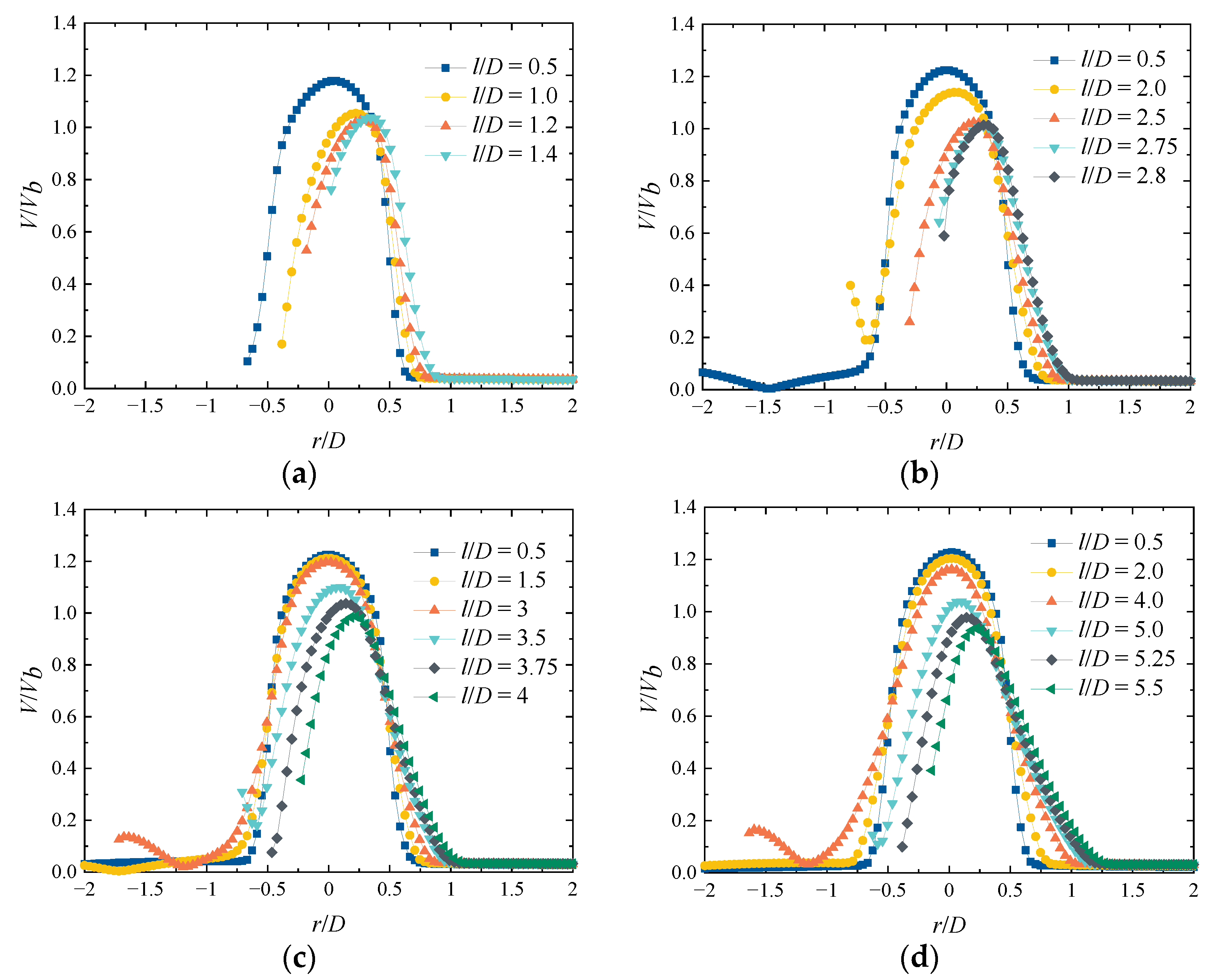
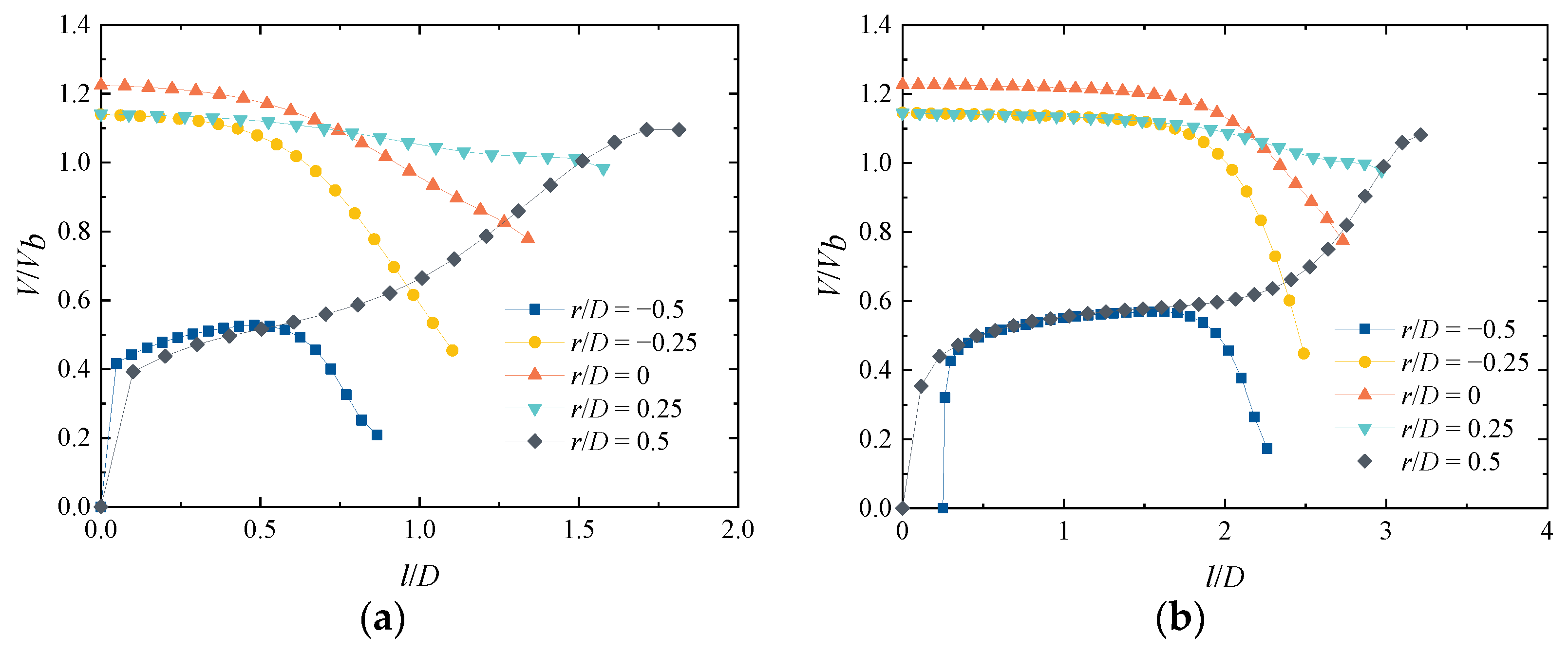
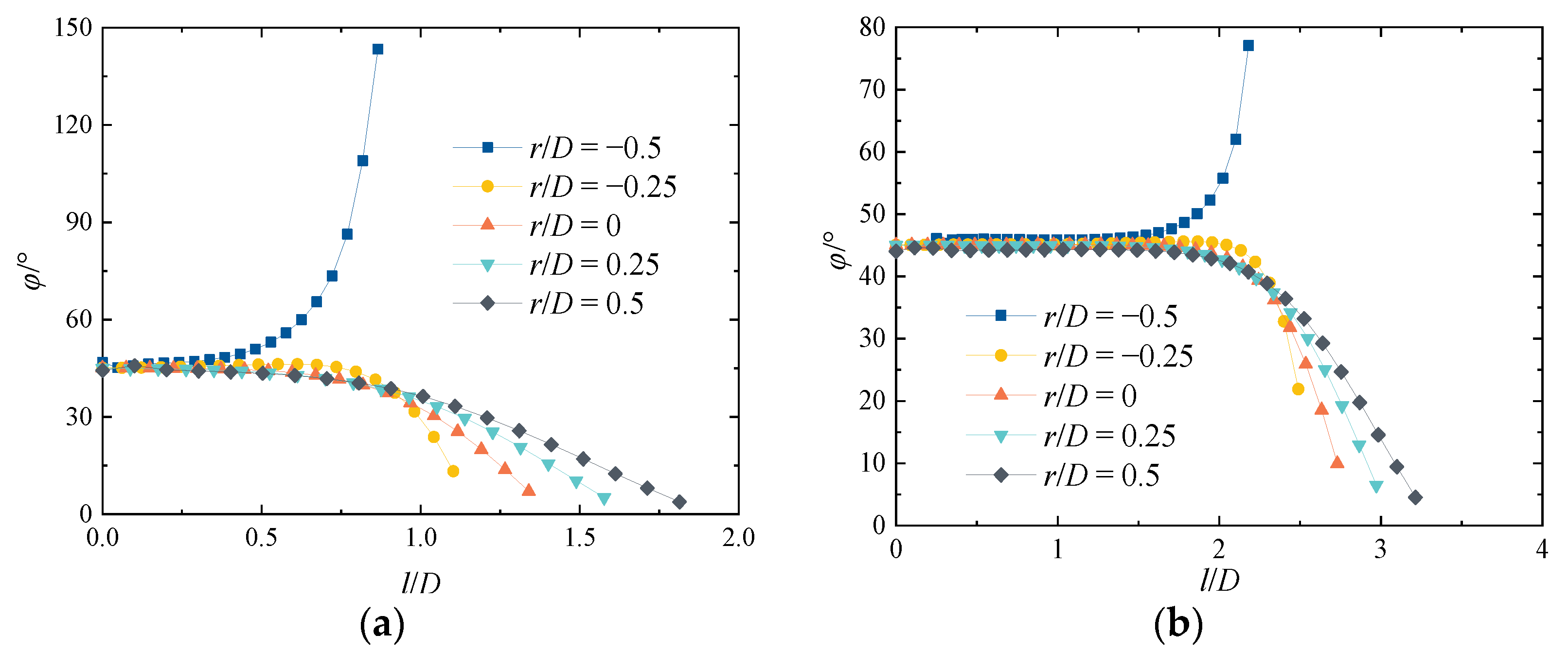
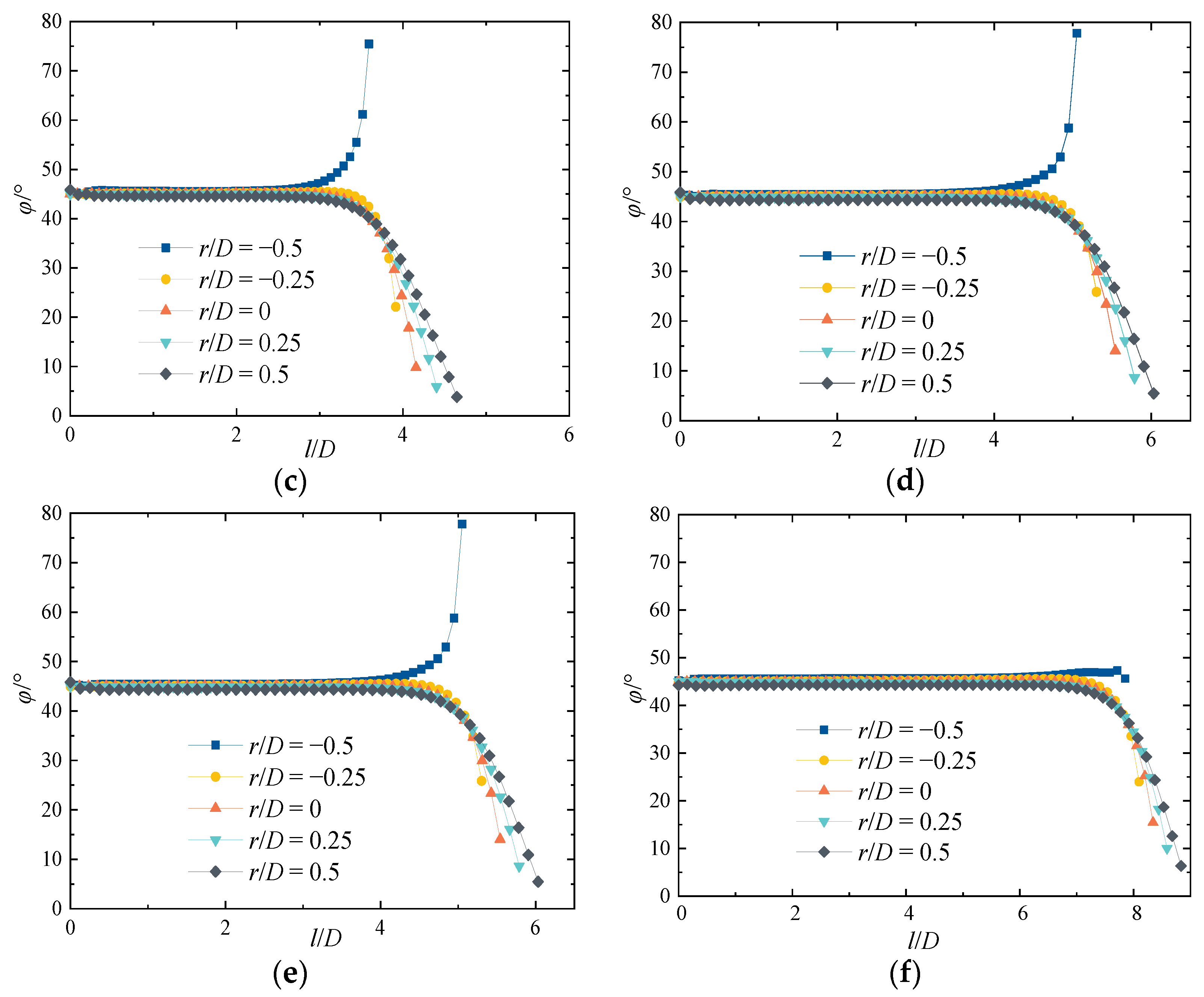
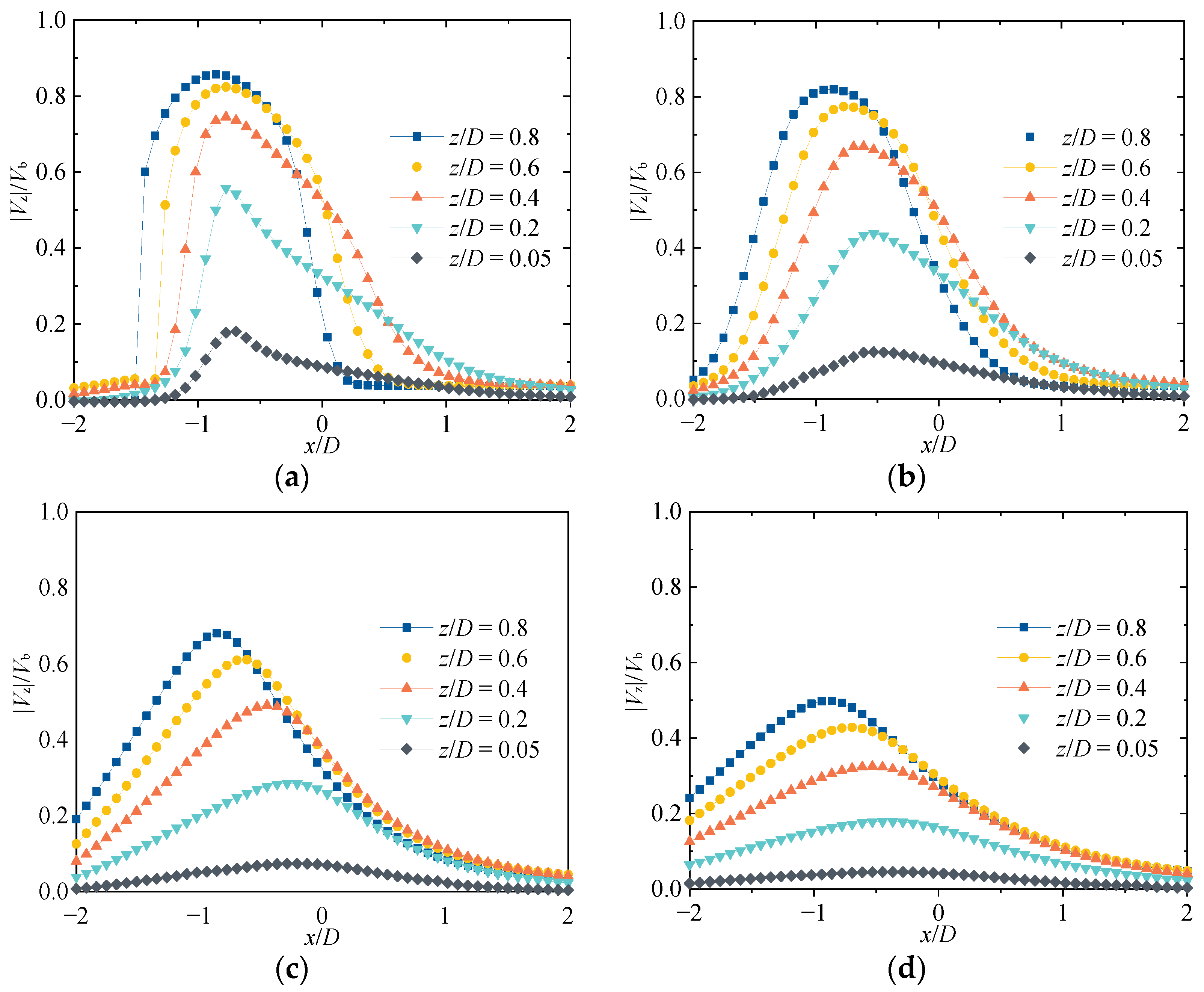
3.2. Mean Velocity Profile in the Near-Wall Region

To highlight the flow structure, the location of the stagnation point (SP) (the segmentation point of the downstream and countercurrent) and the geometric center (GC) (the intersection of the jet pipe center extension line and the impingement plane) are added to the figure. The fluid decelerates rapidly near the impingement plane and begins to develop laterally along the plane, thus forming a wall-jet region, which is mainly composed of a downstream region (+x direction) and a countercurrent region (−x direction). Figure 11 shows the mean velocity vector field (Re = 35,100) of the mid-section (y/D = 0) near-wall region (0 ≤ z/D ≤ 1, −3 ≤ x/D ≤ 3) of the jet at different impinging heights. The increase in impinging height leads to the increase in jet diffusion when reaching the impingement region, and the maximum value of V/V_b decreases; the wall jet thickness increases, and the velocity gradient decreases. When H/D ≤ 3, the location of SP remains unchanged; when H/D > 3, the location of SP gradually moves away from GC.

The horizontal distance between SP and GC is represented by L_sp. Figure 12 shows the L_sp/D distribution at different impinging heights. When H/D ≤ 3, L_sp/D decreases slightly from 0.62 and then increases to 0.6, and the size difference of L_sp/D under different levels of Re is small. When H/D > 3, the value of L_sp/D gradually increases with the increase in H/D. When Re = 11,700, L_sp/D is larger than when Re is higher.

To explore the velocity distribution in the near-wall region, Figure 13 and Figure 14 show the horizontal distributions of |V_z|/V_b and V_x/V_b (Re = 35,100) at different locations (z/D = 0.05, 0.2, 0.4, 0.6, and 0.8) between the jet exit and the impingement plane. As shown in Figure 13, under different impinging heights, the distribution law of |V_z|/V_b at the same section z/D is similar. With the increase in x, |V_z|/V_b increases rapidly and then decreases. In the forward flow direction of jet, the attenuation of |V_z|/V_b is related to the impinging height. When x/D ≥ 1.5, |V_z|/V_b is close to 0, indicating that the mainstream velocity direction of the jet is horizontal. As shown in Figure 14, when 0.6 ≤ z/D ≤ 0.8, the profile of section V_x/V_b is similar, indicating that the velocity V_x/V_b in this region deflects in +x direction, and the velocity is less affected by the impingement plane. When 0.05 ≤ z/D ≤ 0.4, the maximum value of V_x/V_b increases gradually with the decrease in z/D; in the jet’s downstream direction, the jet fluid first accelerates and then decelerates. In the range of x < 0, V_x/V_b has a negative value at section z/D = 0.05, indicating that the jet flows in the countercurrent direction.

The distribution law of the maximum velocity V_m/V_b of the wall jet along the forward flow direction is shown in Figure 15 (Re = 35,100). As shown in the figure, when H/D ≤ 6, there is a large difference in velocity V_m/V_b at various impinging heights in the range of 1 ≤ x/D ≤ 4, and the difference is small in the range of x/D > 4, which is in good agreement with the fitting formula V_m/V_b = 2.3(x/D)⁻¹; when H/D = 8, the calculated results in the range of x/D > 8 are in good agreement with the formula.

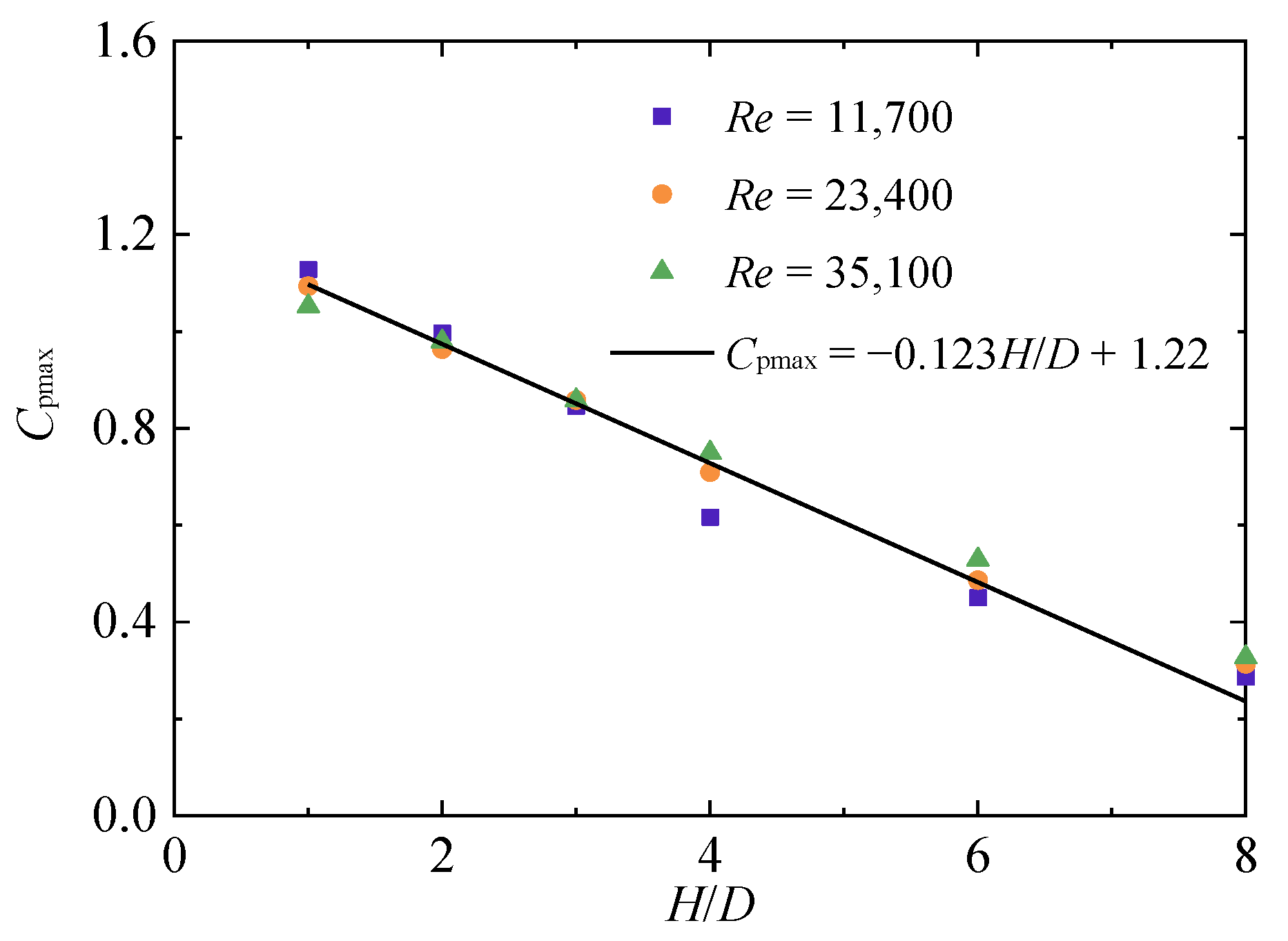
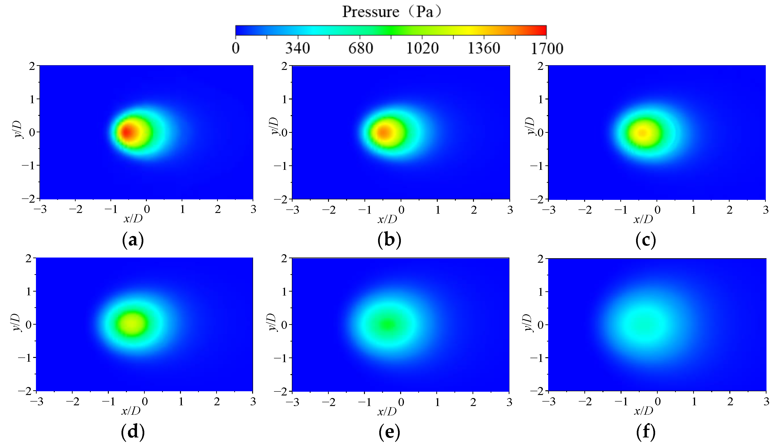
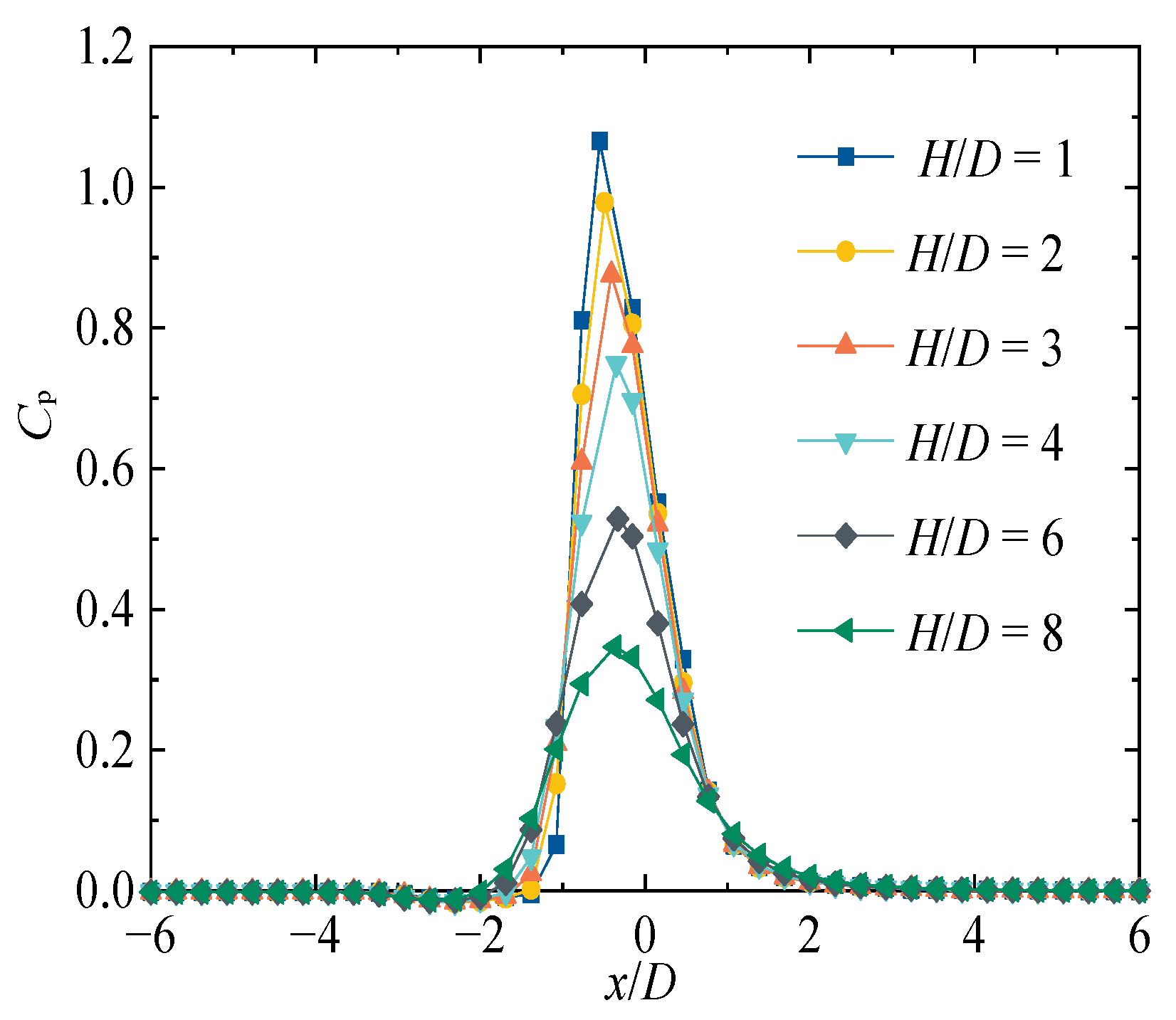
3.3. Time-Averaged Impinging Pressure Distribution

The pressure distribution when the jet impinges on the plane under various heights is shown in Figure 16 (Re = 35,100). When H/D = 1, the pressure distribution on the impingement plane has good symmetry, and the maximum value is obtained at about x/D = −0.5, y/D = 0. The concentration degree of pressure distribution on the left (−x direction) of the maximum pressure point is higher than that on the right. With the increase in impinging height, the maximum impinging pressure on the plane decreases gradually, and the distribution range of the impinging pressure is almost unchanged.

Figure 17 shows the variation law between the maximum pressure coefficient C_pmax and H/D, and gives the fitting formula between them as follows:

$$C_{pmax}=\frac{P_{max}-P_0}{\frac{1}{2}\rho V_b^2}=-0.123\frac{H}{D}+1.22$$

(10)

Figure 18 shows the distribution law of the pressure coefficient at each height. It was found that the pressure coefficient C_p first increases and then decreases with the increase of x, while H/D increases from 1 to 8 and C_pmax decreases from 1.1 to 0.3, but the effective impact range is −2 ≤ x/D ≤ 2, which is independent of the height. With the increase in impinging height, the maximum pressure coefficient gradually decreases, and the C_p curve gradually flattens. In engineering applications, such as electronic component cooling, there is not always the condition of vertical impact heat dissipation. The oblique jet results show that in the studied height range (1 ≤ H/D ≤ 8), the effective impact range is [−2D,2D]. With the increase in impact height, the impact pressure decreases significantly. In practical engineering applications, it is not recommended that the impact height be greater than eight times the pipe diameter. At the same time, the pressure in the center of short-distance impact is large and the pressure on both sides is low. The impact height can be reasonably selected according to the impact region.

4. Conclusions

Oblique submerged impinging jets (θ = 45°) at various heights (1 < H/D < 8) were simulated by using the Wray–Agarwal turbulence model. The following conclusions were obtained through the numerical simulation:

(1) With the increase in impinging height, the diffusion degree of the oblique jet increases gradually, while the velocity decreases when it reaches the impingement region, and the distance between stagnation point (SP) and geometric center (GC) increases gradually.

(2) The flow angle φ along the jet centerline remains constant in the free-jet region and decreases rapidly in the impingement region. The maximum axial velocity V_m/V_b at different locations of the wall-jet region is essentially consistent with the formula V_m/V_b = 2.3(x/D)⁻¹. As the impinging height increases, the size of the vortex in the flow field is almost unchanged, but its intensity gradually weakens.

(3) An increase in impinging height leads to a decrease in the maximum impinging pressure coefficient and pressure coefficient, but the effective impinging pressure is maintained in the range of −2 ≤ x/D ≤ 2. The pressure distribution is similar at various heights, and the impinging pressure concentration on the left (−x direction) of the maximum pressure point is higher.

References

1. Cooper, D.; Jackson, D.C.; Launder, B.E.; Liao, G.X. Impinging jet studies for turbulence model assessment—I. Flow-field experiments. Int. J. Heat Mass Transf. 1993, 36, 2675–2684. [Google Scholar] [CrossRef]
2. Ashforthfrost, S.; Jambunathan, K. Effect of nozzle geometry and semi-confinement on the potential core of a turbulent axisymmetric free jet. Int. Commun. Heat Mass Transf. 1996, 23, 155–162. [Google Scholar] [CrossRef]
3. Alekseenko, S.V.; Bilsky, A.V.; Dulin, V.M.; Markovich, D.M. Experimental study of an impinging jet with different swirl rates. Int. J. Heat Fluid Flow 2007, 28, 1340–1359. [Google Scholar] [CrossRef]
4. Hammad, K.J.; Milanovic, I. Flow structure in the near-wall region of a submerged impinging jet. J. Fluids Eng. 2011, 133, 091205. [Google Scholar] [CrossRef]
5. Xu, Z.; Hangan, H. Scale, boundary and inlet condition effects on impinging jets. J. Wind Eng. Ind. Aerodyn. 2008, 96, 2383–2402. [Google Scholar] [CrossRef]
6. Fitzgerald, J.A.; Garimella, S.V. A study of the flow field of a confined and submerged impinging jet. Int. J. Heat Mass Transf. 1998, 41, 1025–1034. [Google Scholar] [CrossRef]
7. Lai, H.; Naughton, J.W.; Lindberg, W.R. An experimental investigation of starting impinging jets. J. Fluids Eng. 2003, 125, 275–282. [Google Scholar] [CrossRef]
8. Pieris, S.; Zhang, X.; Yarusevych, S.; Peterson, S.D. Vortex dynamics in a normally impinging planar jet. Exp. Fluids 2019, 60, 84. [Google Scholar] [CrossRef]
9. Hanson, G.J.; Robinson, K.M.; Temple, D.M. Pressure and stress distributions due to a submerged impinging jet. In Hydraulic Engineering—Proceedings of the 1990 National Conference, San Diego, CA, USA, 30 July–3 August 1990; Reston, V., Ed.; American Society of Civil Engineers: Reston, VA, USA, 1990; pp. 525–530. [Google Scholar]
10. Yang, Y.; Zhou, L.; Bai, L.; Xu, H.; Lv, W.; Shi, W.; Wang, H. Numerical investigation of tip clearance effects on the performance and flow pattern within a sewage pump. J. Fluids Eng. 2022, 144, 081202. [Google Scholar] [CrossRef]
11. Tang, S.; Zhu, Y.; Yuan, S. Intelligent fault diagnosis of hydraulic piston pump based on deep learning and Bayesian optimization. ISA Trans. 2022; in press. [Google Scholar] [CrossRef] [PubMed]
12. Zhu, Y.; Li, G.; Wang, R.; Tang, S.; Su, H.; Cao, K. Intelligent fault diagnosis of hydraulic piston pump combining improved LeNet-5 and PSO hyperparameter optimization. Appl. Acoust. 2021, 183, 108336. [Google Scholar] [CrossRef]
13. Wang, C.; Shi, W.; Wang, X.; Jiang, X.; Yang, Y.; Li, W.; Zhou, L. Optimal design of multistage centrifugal pump based on the combined energy loss model and computational fluid dynamics. Appl. Energy 2017, 187, 10–26. [Google Scholar] [CrossRef]
14. Wang, C.; Chen, X.; Qiu, N.; Zhu, Y.; Shi, W. Numerical and experimental study on the pressure fluctuation, vibration, and noise of multistage pump with radial diffuser. J. Braz. Soc. Mech. Sci. Eng. 2018, 40, 481. [Google Scholar] [CrossRef]
15. Zhang, D.; Jiao, W.; Cheng, L.; Xia, C.; Zhang, B.; Luo, C.; Wang, C. Experimental study on the evolution process of the roof-attached vortex of the closed sump. Renew. Energy 2021, 164, 1029–1038. [Google Scholar] [CrossRef]
16. Wang, Q.; Huang, Q.; Sun, X.; Zhang, J.; Karimi, S.; Shirazi, S.A. Transient Large Eddy Simulation of Slurry Erosion in Submerged Impinging Jets. J. Energy Resour. Technol. 2021, 143, 062107. [Google Scholar] [CrossRef]
17. Sabato, M.; Fregni, A.; Stalio, E.; Brusiani, F.; Tranchero, M.; Baritaud, T. Numerical study of submerged impinging jets for power electronics cooling. Int. J. Heat Mass Transf. 2019, 141, 707–718. [Google Scholar] [CrossRef]
18. Zerrout, A.; Khelil, A.; Loukarfi, L. Experimental and numerical investigation of impinging multi-jet system. Mechanika 2017, 23, 228–235. [Google Scholar]
19. Abdel-Fattah, A. Numerical simulation of turbulent impinging jet on a rotating disk. Int. J. Numer. Methods Fluids 2007, 53, 1673–1688. [Google Scholar] [CrossRef]
20. So, H.; Yoon, H.G.; Chung, M.K. Large eddy simulation of flow characteristics in an unconfined slot impinging jet with various nozzle-to-plate distances. J. Mech. Sci. Technol. 2011, 25, 721–729. [Google Scholar] [CrossRef]
21. Wang, C.; Wang, X.; Shi, W.; Lu, W.; Tan, S.K.; Zhou, L. Experimental investigation on impingement of a submerged circular water jet at varying impinging angles and Reynolds numbers. Exp. Therm. Fluid Sci. 2017, 89, 189–198. [Google Scholar] [CrossRef]
22. Mishra, A.; Yadav, H.; Djenidi, L.; Agrawal, A. Experimental study of flow characteristics of an oblique impinging jet. Exp. Fluids 2020, 61, 90. [Google Scholar] [CrossRef]
23. Jalil, A.; Rajaratnam, N. Oblique impingement of circular water jets on a plane boundary. J. Hydraul. Res. 2006, 44, 807–814. [Google Scholar] [CrossRef]
24. Jiao, W.; Zhang, D.; Wang, C.; Cheng, L.; Wang, T. Unsteady numerical calculation of oblique submerged jet. Energies 2020, 13, 4728. [Google Scholar] [CrossRef]
25. Wray, T.J.; Agarwal, R.K. Low-Reynolds-number one-equation turbulence model based on k-ω closure. AIAA J. 2015, 53, 2216–2227. [Google Scholar] [CrossRef]
26. Han, X.; Wray, T.J.; Fiola, C.; Agarwal, R.K. Computation of flow in S ducts with Wray–Agarwal one-equation turbulence model. J. Propuls. Power 2015, 31, 1338–1349. [Google Scholar] [CrossRef]
27. Han, X.; Wray, T.; Agarwal, R.K. Application of a new DES model based on wray-agarwal turbulence model for simulation of wall-bounded flows with separation. In Proceedings of the 47th AIAA Fluid Dynamics Conference, Denver, CO, USA, 2 June 2017; p. 3966. [Google Scholar]
28. Wang, H.; Qian, Z.; Zhang, D.; Wang, T.; Wang, C. Numerical study of the normal impinging water jet at different impinging height, based on Wray–Agarwal turbulence model. Energies 2020, 13, 1744. [Google Scholar] [CrossRef] [Green Version]
Figure 1. Establishment of calculation model coordinate system: (a) three-dimensional diagram of oblique submerged water jet; (b) schematic diagram of the flow angle φ on the o2xz section.
Jmse 10 00399 g001
Figure 2. Computational grid generation and independence verification: (a) calculation grid of oblique submerged jet; (b) analysis of grid independence.
Jmse 10 00399 g002
Figure 3. Comparison of axial velocity profiles of jet exit section.
Jmse 10 00399 g003
Figure 4. Streamline diagram of oblique submerged impinging jet at various impinging heights: (a) H/D = 1; (b) H/D = 2; (c) H/D = 3; (d) H/D = 4; (e) H/D = 6; (f) H/D = 8.
Jmse 10 00399 g004
Figure 5. Normalized mean velocity V/Vb cloud chart and streamline of mid-section at various impinging heights: (a) H/D = 1; (b) H/D = 2; (c) H/D = 3; (d) H/D = 4; (e) H/D = 6; (f) H/D = 8.
Jmse 10 00399 g005
Figure 6. Normalized mean velocity V/Vb cloud chart and streamline of different cross sections at various impinging height: (a) H/D = 1; (b) H/D = 2; (c) H/D = 3; (d) H/D = 4; (e) H/D = 6; (f) H/D = 8.
Jmse 10 00399 g006aJmse 10 00399 g006b
Figure 7. Normalized mean axial (V/Vb), horizontal (|Vx|/Vb), and vertical (|Vy|/Vb) velocity profiles along the centerline of the impinging jet at various impinging heights: (a) H/D = 1; (b) H/D = 8.
Jmse 10 00399 g007
Figure 8. Radial profile development of the normalized mean axial velocity V/Vb at various impinging heights: (a) H/D = 1; (b) H/D = 2; (c) H/D = 3; (d) H/D = 4; (e) H/D = 6; (f) H/D = 8.
Jmse 10 00399 g008aJmse 10 00399 g008b
Figure 9. Axial profile development of mean velocity V/Vb at different radial locations under various impinging heights: (a) H/D = 1; (b) H/D = 2; (c) H/D = 3; (d) H/D = 4; (e) H/D = 6; (f) H/D = 8.
Jmse 10 00399 g009aJmse 10 00399 g009b
Figure 10. Development of flow angle φ along the axial direction at different radial locations under various impinging heights: (a) H/D = 1; (b) H/D = 2; (c) H/D = 3; (d) H/D = 4; (e) H/D = 6; (f) H/D = 8.
Jmse 10 00399 g010aJmse 10 00399 g010b
Figure 11. Mean velocity vectors in the near-wall region and flood contours of the normalized mean axial velocity V/Vb: (a) H/D = 1; (b) H/D = 2; (c) H/D = 3; (d) H/D = 4; (e) H/D = 6; (f) H/D = 8.
Jmse 10 00399 g011aJmse 10 00399 g011b
Figure 12. Normalized distance Lsp/D between SP and GC.
Jmse 10 00399 g012
Figure 13. Development of mean vertical velocity (|Vz|/Vb) along the horizontal direction at different vertical locations on the near-well region: (a) H/D = 1; (b) H/D = 3; (c) H/D = 6; (d) H/D = 8.
Jmse 10 00399 g013
Figure 14. Development of mean horizontal velocity (Vx/Vb) along the horizontal direction at different vertical locations on the near-well region: (a) H/D = 1; (b) H/D = 3; (c) H/D = 6; (d) H/D = 8.
Jmse 10 00399 g014aJmse 10 00399 g014b
Figure 15. Variation of normalized maximum velocity Vm/Vb of the wall jet along the forward flow direction.
Jmse 10 00399 g015
Figure 16. Pressure contour of jet impingement plane (oxy plane) under various impinging heights: (a) H/D = 1; (b) H/D = 2; (c) H/D = 3; (d) H/D = 4; (e) H/D = 6; (f) H/D = 8.
Jmse 10 00399 g016
Figure 17. Variation of the maximum pressure coefficient Cpmax as a function of H/D.
Jmse 10 00399 g017
Figure 18. Variation of pressure coefficient Cp along the x-axis at various impinging heights.
Jmse 10 00399 g018
Publisher’s Note: MDPI stays neutral with regard to jurisdictional claims in published maps and institutional affiliations.