Robust Path-Following Control of Underactuated AUVs with Multiple Uncertainties in the Vertical Plane

Abstract

The current study employs a novel nonlinear robust control approach for path-following control of underactuated autonomous underwater vehicles (AUVs) with multiple uncertainties in the vertical plane. Firstly, a nonlinear underactuated AUV model is established to characterize the dynamics of AUV and path-following error. To resolve dependence on a detailed model that appeared in previous studies, the unknown time-varying attack angular velocity in the dynamic model of the path-following error is considered as the kinematic uncertainty, while the linear superposition of the external environmental disturbances, the perturbations in the internal model parameters, and other unmodeled dynamics in the dynamic model is chosen as lumped dynamic uncertainties. Several reduced-order extended state observers (ESOs) are designed for estimating both of these uncertainties. Secondly, to reduce the impact of input saturation and avoid the “explosion of complexity” associated with traditional back-stepping method, a nonlinear track differentiator (NTD) is utilized to follow the virtual control signal and its derivative. Thirdly, the constructed reduced-order ESOs and NTD are adopted to establish an augmented back-stepping controller, where its ability to stabilize the overall system is demonstrated using the Lyapunov theorem. Finally, extensive simulations and analyses in various working conditions, including the nominal working condition without disturbances, the working condition with multiple uncertainties, and the conditions which better replicate the actual environment, are performed to demonstrate the effectiveness, superiority, and robustness of the designed controller.

1. Introduction

With the growth of marine operations, autonomous underwater vehicles (AUVs) have become valuable tools in various applications, including water quality control, geological sampling, underwater archaeology, underwater rescue, and oceanographic surveys [1,2,3,4,5]. During the mission execution mentioned above, various studies in recent decades have been devoted to the path-following control of an AUV [6,7]. The path-following issue involves establishing control strategies that allow a marine vehicle to track the desired trajectory without time limitations [8,9]. The vehicle configuration determines the complexity of the above-mentioned problem. For example, the path-following of an entirely actuated vehicle is a straightforward problem. However, due to the weight, reliability, complexity, and performance requirements, most popular AUVs are underactuated with fewer inputs than degrees of freedom (DOFs). Lack of sway and heave actuation make the design of the control system highly complicated, since most of the underactuated systems are strongly coupled, time-varying, inherently extremely nonlinear among the movement of multiple DOFs, and include non-integrable acceleration constraints [10,11]. Additionally, the working environments of an underactuated AUV often bring unpredictable disturbances, such as internal parametric uncertainties and external environmental disturbances, to the control system, which might result in slow convergence speeds, or/and large steady-state errors, and even cause instability of the closed-loop system [12].

In order to maintain stability and improve robustness in the presence of multiple disturbances, many control strategies such as back-stepping control [13,14], sliding mode control (SMC) [15,16], fuzzy control [17], neural network control [18,19], observer-based method [20,21], model predictive control (MPC) [22], and their combinations [23,24] have been widely utilized for path-following control of underactuated AUVs. In [25], an adaptive switching supervisory control method was utilized to solve the trajectory-tracking problems of underactuated vehicles suffering from large parametric uncertainties. In [26], a hybrid parameter tuning strategy had been used to enhance the vehicle robustness, and the proposed standard adaption strategy can only deal with the dynamic parameters in an affine structure. In [18], dynamic surface control was adopted to design the controller, and a neural network was employed to estimate the model uncertainties in the hydrodynamic damping terms of underactuated AUVs. In [27], Lyapunov’s direct approach, back stepping, and parameter projection strategies were adopted to establish a nonlinear robust adaptive control scheme, forcing a 6-DOF underactuated AUV to follow the predefined path at an intended speed under environmental disturbances. Unfortunately, unknown parameters must be held constant in this method, which is unrealistic for the challenging marine environmental conditions. In [28], the back-stepping approach and dynamical SMC theory were utilized to construct a nonlinear path-following controller for an underactuated surface ship. Although the modeling errors and external disturbances were considered in the control system, the path curvature was not considered. Accordingly, only straight or piecewise straight lines could be followed. By converting the trajectory tracking control problem into a constrained standard quadratic programming problem, Zhang et al. [22] proposed a novel three-dimensional trajectory tracking controller using MPC to address the trajectory tracking problem of an AUV with the model uncertainties and time-varying disturbances. However, the MPC methods require an accurate mathematical model of the vehicle. As is well known, it is challenging to obtain an accurate mathematical model of underactuated AUV due to the complex marine environment.

In practice application, due to the existence of the perturbations in the internal model parameters and the external disturbances, it is an arduous task to perform precise path-following control of an underactuated AUV. In recent years, extended state observer (ESO) has been well developed to estimate the internal model uncertainties and/or the external environmental disturbances [29,30]. Compared to other currently available observer techniques, such as the unknown input observer (UIO), the uncertainty and disturbance estimator (UDE), and other disturbance and uncertainty estimation techniques, it has been proved that ESO requires minimum information about a dynamical system [31]. Therefore, it is appealing to utilize ESO to estimate the unknown velocity and disturbances in the underactuated AUVs [32,33,34]. In [33], an ESO-based disturbance rejection method, combined with neurodynamic optimization method, was proposed for path-following control of underactuated AUVs with velocity and input constraints, as well as internal and external disturbances. Unfortunately, due to the relatively complex derivations and decision-making process, the above-mentioned controller required substantial computational costs. In [35], a finite-time controller based on disturbance observer and command filter back-stepping was proposed to avoid the differential expansion problem caused by the traditional back-stepping calculation complexity. However, the parameter uncertainties were not taken into consideration in the above control method, which is unrealistic in practical applications.

Motivated by the above considerations, a back-stepping controller augmented by reduced-order ESOs and NTD is designed to achieve path-following control of an underactuated AUV with multiple uncertainties in the vertical plane. The main contributions of the current study are summarized as follows:

(1)

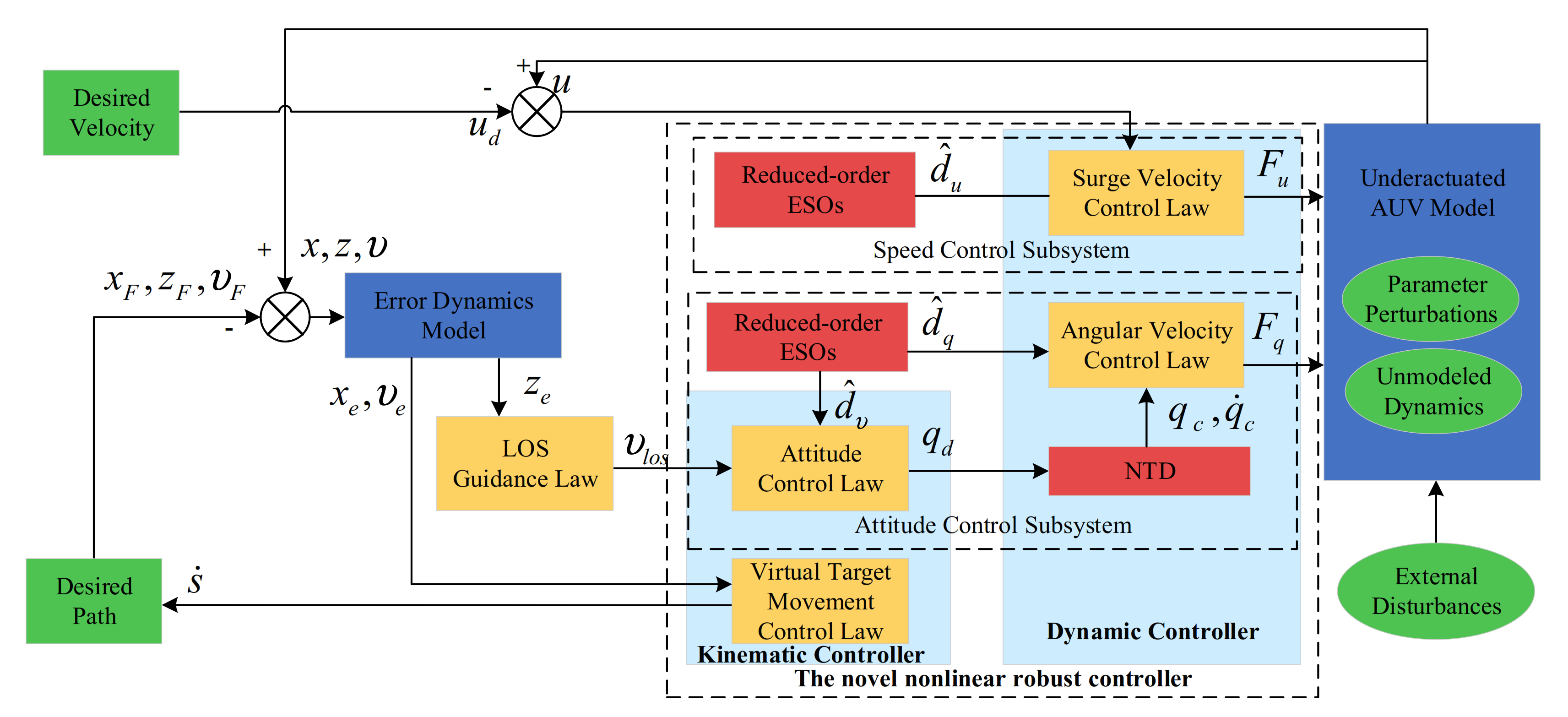
To relax the requirement of having an accurate estimation of the model parameters, and reduce dependence on the precise mathematical model, the unknown time-varying attack angular velocity in the dynamic model of the path-following error is treated as kinematic uncertainty, while the linear superposition of the external environment disturbances, the perturbations in the internal model parameters, and other unmodeled dynamics in the dynamic model is treated as the lumped dynamic uncertainties. Four reduced-order ESOs are introduced for an accurate estimation of the kinematic and dynamic uncertainties. Compared with previous studies [36,37], which are based on the assumption that the attack angle was neglected or regarded as constant, the unknown time-varying attack angle is considered in this paper, which is suitable for a challenging marine environment.

(2)

To eliminate the effect of input saturation and handle the “explosion of complexity” associated with a traditional backstepping method, an NTD is utilized to track the virtual control signal and its derivative. Compared with the traditional dynamic surface control method presented in [18,38], the NTD is a time-optimal solution that provides the fastest tracking of the input signal [29].

(3)

Based on the constructed reduced-order ESOs and NTD, an augmented back-stepping controller is constructed to enhance the robustness against the external environment disturbances, the perturbations in the internal model parameters, and other unmodeled dynamics. Compared with the previous study [39] on vertical path-following control of underactuated AUVs, the proposed controller is simplified and is more suitable for underactuated AUVs cruising in complex marine environment. Then, the nominal working condition without disturbances, the working condition with multiple uncertainties, and the conditions which better replicate the actual environment are introduced to further evaluate the effectiveness, superiority, and robustness of the mentioned controller.

This paper is organized as follows: Section 2 introduces the underactuated AUV dynamics and problem formulation, and the nonlinear path-following control strategy is described in Section 3. In Section 4, the closed-loop system stability is verified, followed by the numerical simulations and discussions provided in Section 5. Section 6 contains the concluding remarks of this paper and future research avenues.

2. Underactuated AUV Model and Problem Formulation

In this section, the three-DOF mathematical model of an underactuated AUV with multiple uncertainties in the vertical plane is presented to formulate the path-following control problem. The path-following problem in the vertical plane is described in Figure 1, where the notations and the corresponding description are presented in

Table 1. Notation.

$\left\{\mathrm{I}\right\}$	Earth-fixed frame
$\left\{\mathrm{B}\right\}$	Body-fixed frame
$\left\{\mathrm{SF}\right\}$	Serret-Frenet frame
$\left[x,z,\theta \right]$	Inertial position and orientation vectors of AUV
$\left[u,w,q\right]$	Body-fixed velocity vector
$\left[x_e,z_e,{\upsilon }_e\right]$	Path following error vector
$\left[x_F,z_F,{\upsilon }_F\right]$	Position and elevation angle vector of virtual target P
$\alpha$	Attack angle of AUV
$\upsilon$	Course angle of AUV
$U$	Total speed of AUV
$\Delta$	Look-ahead distance
${\upsilon }_{LOS}$	Line-of-sight (LOS) angle

.

2.1. The Underactuated AUV Model

The kinematic relations can be described as [17,39]:

$$\left\{\begin{array}{c}\dot{x}=u\cos \theta +w\sin \theta \hfill \\ \dot{z}=-u\sin \theta +w\cos \theta \hfill \\ \dot{\theta }=q\hfill \end{array}\right.$$

(1)

Based on the previous studies [17,39] and considering the external environmental disturbances, the perturbations in the internal model parameters and other unmodeled dynamics, the dynamic model of an underactuated AUV in the vertical plane is modified as:

$$\left\{\begin{array}{c}\dot{u}=F_{11}(u,w,q)+\frac{F_u}{m_{11}}+d_u\hfill \\ \dot{w}=F_{12}(u,w,q)+d_w\hfill \\ \dot{q}=F_{13}(u,w,q)-\frac{BL\sin \theta }{m_{33}}+\frac{F_q}{m_{33}}+d_q\hfill \end{array}\right.$$

(2)

with

$$\begin{gathered} F_{11}\left(u,w,q\right)=-\frac{m_{22}}{m_{11}}wq-\frac{d_{11}}{m_{11}}u-\frac{d_{u2}}{m_{11}}u\left|u\right|-\frac{d_{u3}}{m_{11}}{u}^3 \\ {F}_{12}(u,w,q)=\frac{m_{11}}{m_{22}}uq-\frac{d_{22}}{m_{22}}w-\frac{d_{w2}}{m_{22}}w\left|w\right|-\frac{d_{w3}}{m_{22}}{w}^3 \\ {F}_{13}(u,w,q)=\frac{m_{22}-m_{11}}{m_{33}}uw-\frac{d_{33}}{m_{33}}q-\frac{d_{q2}}{m_{33}}q\left|q\right|-\frac{d_{q3}}{m_{33}}{q}^3 \end{gathered}$$

where $m_{ii}(i=1,2,3)$ denotes the combined terms of mass and inertia parameters of the AUV; $d_{ii}(i=1,2,3)$, $d_{i2}(i=u,w,q)$, and $d_{i3}(i=u,w,q)$ represent the nominal hydrodynamic parameters in the vehicle model; $B$ is the buoyancy of the AUV; $L$ denotes the metacentric height; $F_u$ and $F_q$ represent surge control force and pitch control torque, respectively; $d_i(i=u,w,q)$ represents lumped dynamic uncertainties, including the external environmental disturbances, the perturbations in the internal model parameters and other unmodeled dynamics.

Remark 1.

It is noted that there is no direct control force in the heave direction, so the vehicle is considered underactuated.

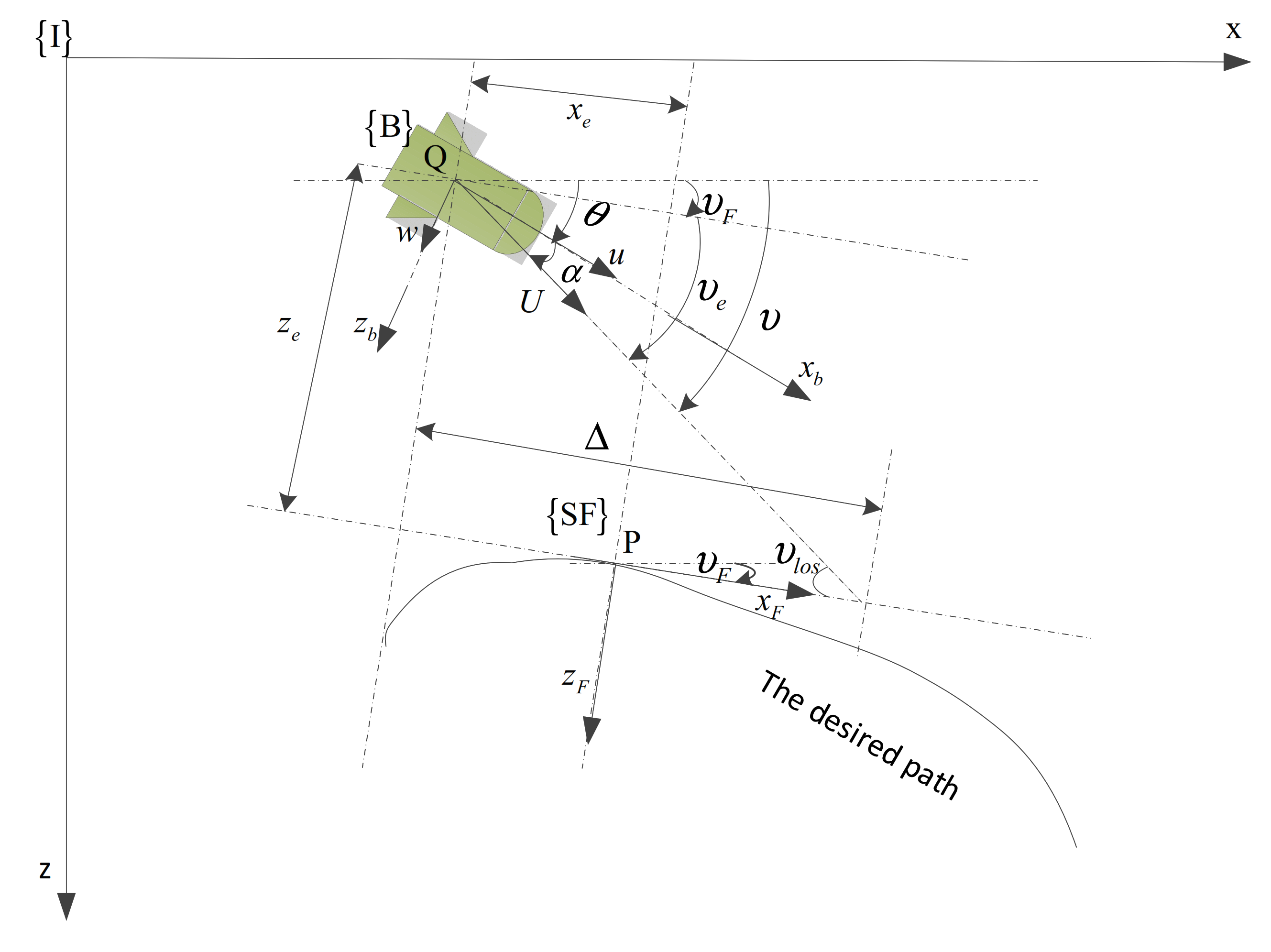
2.2. Path-Following Error Dynamics

As depicted in Figure 1, assuming that an underactuated AUV to track a predefined path is located at $(x,z)$, the path-following error equation constructed in the Serret-Frenet frame is given by [17]:

$$\left\{\begin{array}{l}{x}_e=(x-x_F)\cos {\upsilon }_F-(z-z_F)\sin {\upsilon }_F\\ z_e=(x-x_F)\sin {\upsilon }_F+(z-z_F)\cos {\upsilon }_F\\ {\upsilon }_e=\upsilon -{\upsilon }_F\end{array}\right.$$

(3)

Differentiating the above error equation and considering ${\dot{\upsilon }}_F=c_c(s)\dot{s}, \upsilon =\theta -\alpha$, the error dynamics can be written as follows [17]:

$$\left\{\begin{array}{l}{\dot{x}}_e=-\dot{s}\left(1+z_e{c}_c\right)+U\cos {\upsilon }_e\\ {\dot{z}}_e=c_c\dot{s}{x}_e-U\sin {\upsilon }_e\\ {\dot{\upsilon }}_e=q-\dot{\alpha }-c_c\dot{s}\end{array}\right.$$

(4)

where $c_c(s)$ denotes the path curvature of the predefined path. $\dot{s}$ represents the velocity of the virtual point P.

Remark 2.

It is noted that the third equation of the error dynamic model (Equation (4)) involves the calculation of$\dot{\alpha }$. According to the definition of the attack angle$\alpha =\arctan \left(w/u\right)$and the total speed$U=\sqrt{u^2+w^2}$, it can be deduced that$\dot{\alpha }=(u\dot{w}-w\dot{u})/U^2$. However, due to the existence of the lumped dynamic uncertainties$d_i(i=u,w,q)$, and cannot be obtained from the dynamic model (Equation (2)). Thus,$\dot{\alpha }$is unknown and coupled with the pitch speed$q$. To address this problem,$\dot{\alpha }$is treated as the kinematic uncertainty, and the reduced-order ESO is utilized to observe it.

The third equation of the dynamic model of the path-following error is modified as:

$${\dot{\upsilon }}_e=q-d_{\upsilon }-c_c\dot{s}$$

(5)

where $d_{\upsilon }=\dot{\alpha }$ is the kinematic uncertainty to be estimated.

2.3. Problem Formulation

To facilitate the design of the path-following controller, the reasonable assumptions taken into consideration are summarized as follows:

Assumption 1.

$d_{\upsilon }$ and ${\dot{d}}_{\upsilon }$are bounded, i.e.,$\left|\frac{d^l{d}_{\upsilon }}{d{t}^l}\right|\le {\overline{d}}_{\upsilon } (l=0,1)$, where ${\overline{d}}_{\upsilon }$is an unknown positive constant [34,40].

Assumption 2.

The unknown time-varying lumped dynamic uncertainties are bounded, i.e.,$d_u$, $d_w$, and$d_q$satisfy$‖d_i‖\le {\overline{d}}_i, (i=u,w,q)$, where${\overline{d}}_i(i=u,w,q)$is unknown positive constants [41].

Assumption 3.

A finite desired path is considered, such that$x_F$, $z_F$,${\dot{x}}_F$, and${\dot{z}}_F$are bounded [41].

Assumption 4.

The position vector$(x,z)$, the velocity vector$(u,w,q)$, and the pitch angle$\theta$are measurable.

Remark 3.

Firstly, the kinematic uncertainty$d_{\upsilon }$is determined by$\dot{\alpha }$, and the limited external disturbances mainly influence the attack angle$\alpha$. Therefore, it is reasonable to assume that the$d_{\upsilon }$and${\dot{d}}_{\upsilon }$are bounded in Assumption 1. Secondly, since external disturbances, the perturbations in the internal model parameters, and unmodeled dynamics are bounded in practice, Assumption 2 is reasonable. Finally, due to the limited movement space of AUV, Assumption 3 is practical.

According to the above assumptions and analyses, the formulation of the control objective of the current research can be described as follows:

Considering the dynamics of AUV and path-following error dynamics described by Equations (2) and (4), design an appropriate controller which can force the underactuated AUV to follow a given geometric path at the desired surge speed $u_d$ in the limitations described by Assumptions 1–4, such that

$$\underset{t\in \left[t_0,\infty \right]}{\sup }‖x_e‖\le \epsilon , \underset{t\in \left[t_0,\infty \right]}{\sup }‖z_e‖\le \epsilon , \underset{t\in \left[t_0,\infty \right]}{\sup }‖{\upsilon }_e-{\upsilon }_{LOS}‖\le \epsilon , \underset{t\in \left[t_0,\infty \right]}{\sup }‖u-u_d‖\le \epsilon$$

where $\epsilon$ is a small positive constant and desired bound among the controlled output and the reference signal.

3. Path-Following Controller Design

In this section, a novel robust path-following control scheme for the underactuated AUV subject to multiple uncertainties is established. The structure of the proposed controller is shown in Figure 2. The nonlinear controller can be divided into two parts: speed control subsystem and attitude control subsystem. Two sets of reduced-order ESOs are designed to estimate the kinematic and dynamic uncertainties, and the estimated values are used in the design of the speed control subsystem and the attitude control subsystem. In the attitude control subsystem, the attitude control law is designed to generate the desired pitch angular velocity. Then, the angular velocity control law is designed to generate the pitch moment, so that the pitch angular velocity can converge to the desired pitch angular velocity. To resolve the problem of “explosion of complexity” inherent in the traditional back-stepping method, the NTD is utilized to obtain the derivative of the desired pitch angular velocity. In the speed control subsystem, the surge velocity control law is designed to generate the surge force, so that the surge speed can converge to the desired surge speed.

3.1. Design of Reduced-Order ESOs

As mentioned previously, the advantage of an ESO is that it needs only the minimum effective information of the dynamical system [32]. Moreover, compared with the conventional ESO, the reduced-order ESO produces faster transient response in the same bandwidth [42]. Therefore, four reduced-order ESOs are designed for estimating the kinematic uncertainty $d_{\upsilon }$ in the dynamic model of the path-following error and lumped dynamic uncertainties $d_i(i=u,w,q)$ in the dynamic model. The following four specific reduced-order ESOs are designed as follows [30]:

$$\left\{\begin{array}{l}{\dot{p}}_1=-{\omega }_1{p}_1-{\omega }_1^{2}u-{\omega }_1\left[\frac{F_u}{m_{11}}+F_{11}\left(u,w,q\right)\right]\\ {\widehat{d}}_u={\omega }_{1}u+p_1 , {\omega }_1>0\end{array}\right.$$

(6a)

$$\left\{\begin{array}{l}{\dot{p}}_2=-{\omega }_2{p}_2-{\omega }_2^{2}w-{\omega }_2{F}_{12}\left(u,w,q\right)\\ {\widehat{d}}_w={\omega }_{2}w+p_2 , {\omega }_2>0\end{array}\right.$$

(6b)

$$\left\{\begin{array}{l}{\dot{p}}_3=-{\omega }_3{p}_3-{\omega }_3^{2}q-{\omega }_3\left[F_{13}\left(u,w,q\right)-\frac{BL\sin \theta }{m_{33}}+\frac{F_q}{m_{33}}\right]\\ {\widehat{d}}_q={\omega }_{3}q+p_3 , {\omega }_3>0\end{array}\right.$$

(6c)

$$\left\{\begin{array}{l}{\dot{p}}_4=-{\omega }_4{p}_4-{\omega }_4^2{\upsilon }_e-{\omega }_4\left(q-c_c\dot{s}\right)\\ {\widehat{d}}_{\upsilon }=-\left({\omega }_4{\upsilon }_e+p_4\right) , {\omega }_4>0\end{array}\right.$$

(6d)

where ${\widehat{d}}_u$, ${\widehat{d}}_w$, ${\widehat{d}}_q$, and ${\widehat{d}}_{\upsilon }$ are estimations of the dynamic and kinematic uncertainties, $p_i(i=1,2,3,4)$ denotes the observe auxiliary state, and ${\omega }_i(i=1,2,3,4)$ describes the bandwidth of reduced-order ESOs.

Remark 4.

Considering that the internal dynamics$F_{11}$, $F_{12}$, and $F_{13}$are available before design, their models are included in the observers to reduce its estimation burden.

The estimation error of reduced-order ESOs for disturbances has been widely investigated in previous studies [42]. Therefore, the following conclusion can be obtained [43]:

$$‖E_0‖\le \frac{\max ({\overline{d}}_j)}{\min (\left|{\omega }_i\right|)}, j=u,w,q,\upsilon , i=1,2,3,4$$

(7)

where $E_0={[\begin{array}{cccc}{\tilde{d}}_u& {\tilde{d}}_w& {\tilde{d}}_q& {\tilde{d}}_{\upsilon }\end{array}]}^T={[\begin{array}{cccc}{d}_u-{\widehat{d}}_u& d_w-{\widehat{d}}_w& d_q-{\widehat{d}}_q& d_{\upsilon }-{\widehat{d}}_{\upsilon }\end{array}]}^T$.

Remark 5.

Equation (7) indicates that the observer gains${\omega }_i(i=1,2,3,4)$can be adjusted to ensure the estimation errors is within an arbitrarily narrow bound.

3.2. The LOS Guidance Law Design

In this subsection, the LOS guidance law is constructed to calculate the desired LOS angle. The LOS guidance issue and the interrelated essential variables are described in Figure 1. The maneuvering features of the vehicle change significantly concerning the look-ahead distance $(\Delta )$. Hence, algorithms with a time-varying $\Delta$ are implemented to ensure flexible behavior. Here, in order to reduce the overall complexity of the problem, a fixed $\Delta$ is considered and the LOS guidance law is given by:

$${\upsilon }_{LOS}=\arctan \left(\frac{z_e}{\Delta }\right), \Delta >0$$

(8)

Remark 6.

The value of$\Delta$affects the guidance performance, for instance, a lower value of$\Delta$induces more aggressive steering, whereas a larger value of$\Delta$induces milder steering. Therefore, the value of$\Delta$is usually chosen between 1.5 and 2.5 of the AUV length.

3.3. The Kinematic Controller Design

3.3.1. The Virtual Target Movement Control Law Design

In this subsection, the virtual target movement control law is constructed to overcome the strict constraints that the initial position of the underactuated AUV must be in a narrow bound near the desired path. As proposed in [26,44], the virtual target movement control law is constructed as follows:

$$\dot{s}=U\cos {\upsilon }_e+k_2{x}_e$$

(9)

where $k_2$ is a positive constant.

3.3.2. Attitude Control Law Design

In this subsection, the attitude control law is constructed to calculate the desired pitch speed $q_d$. The desired dynamic features of the pitch angle error ${\upsilon }_e$ can be represented as follows:

$${\dot{\upsilon }}_e={\dot{\upsilon }}_{LOS}-k_1({\upsilon }_e-{\upsilon }_{LOS})$$

(10)

where $k_1$ is a positive constant.

According to the linear feedback design process, inserting Equation (10) into Equation (5), results in:

$$q_d=c_c\dot{s}+{\dot{\upsilon }}_{LOS}+d_{\upsilon }-k_1({\upsilon }_e-{\upsilon }_{LOS})$$

(11)

where $q_d$ denotes the desired pitch speed.

With the kinematic uncertainty obtained by the reduced-order ESO (Equation (6d)), the desired pitch speed can be modified as:

$$q_d=c_c\dot{s}+{\dot{\upsilon }}_{LOS}+{\widehat{d}}_{\upsilon }-k_1({\upsilon }_e-{\upsilon }_{LOS})$$

(12)

3.4. Dynamic Controller Design

3.4.1. Angular Velocity Control Law Design

In this subsection, the angular velocity control law is constructed to generate the control moment $F_q$, so that the pitch speed $q$ can converge to the desired pitch speed $q_d$ obtained by the attitude control law. The desired dynamics of pitch speed can be represented as follows:

$$\dot{q}={\dot{q}}_d-k_4(q-q_d)$$

(13)

where $k_4$ is a positive constant.

Substituting Equation (13) into the third equation of Equation (2), together with the estimation ${\widehat{d}}_q$ generated by the ESO (Equation (6c)), the angular velocity control law can be obtained as:

$$F_q=\left[-k_4\left(q-q_d\right)+{\dot{q}}_d-{\widehat{d}}_q-F_{13}\left(u,w,q\right)\right]m_{33}+BL\sin \theta$$

(14)

It is noted that the angular velocity control law represented by Equation (14) involves the calculation of the derivative (${\dot{q}}_d$) of the desired pitch angle $q_d$. However, the complex expression ${\widehat{d}}_{\upsilon }$ (Equation (6d)) is included in $q_d$, which results in the problem of “explosion of complexity”. Therefore, an NTD is introduced to obtain the derivative of the desired pitch speed. The discrete form of NTD is provided as follows [29]:

$$\left\{\begin{array}{l}fh=fhan(q_c(k)-q_d(k),{\dot{q}}_c(k),r,h)\\ q_c(k+1)=q_c(k)+T{\dot{q}}_c(k)\\ {\dot{q}}_c(k+1)={\dot{q}}_c(k)+Tfh\end{array}\right.$$

(15)

where $q_c$ is the fastest tracking of $q_d$ and ${\dot{q}}_c$ is the derivative of $q_c$; $T$ denotes the sampling period, $r$ is an acceleration parameter, and $h$ is the filter factor. A description of $fhan(\cdot )$ and a detailed explanation about the NTD have been presented in [29].

The theoretical results about the NTD convergence in [30,43] can be utilized to derive the following results:

Corollary 1.

If the input signal $q_d$is differentiable and bounded, there are arbitrarily small values of$a,{\epsilon }_1,{\epsilon }_2>0$, such that:

$$\left\{\begin{array}{l}\underset{q\to \infty }{\lim }\left|q_c-q_d\right|\le {\epsilon }_1\\ \underset{q\to \infty }{lim}\left|{\dot{q}}_c-{\dot{q}}_d\right|\le {\epsilon }_2\end{array}\right.t\in [a,\infty )$$

(16)

Therefore, with the availability of $q_c$ and its derivative ${\dot{q}}_c$, the angular velocity control law (Equation (14)) can be further modified as:

$$F_q=\left[-k_4\left(q-q_c\right)+{\dot{q}}_c-{\widehat{d}}_q-F_{13}\left(u,w,q\right)\right]m_{33}+BL\sin \theta$$

(17)

3.4.2. Surge Velocity Control Law Design

In this subsection, the surge velocity control law is constructed to generate the control force $F_u$, so that the surge speed $u$ can converge to the given desired surge speed $u_d$. The desired dynamics of the surge speed can be represented as follows:

$$\dot{u}={\dot{u}}_d-k_3(u-u_d)$$

(18)

where $k_3$ is a positive constant and ${\dot{u}}_d=0$.

Substituting Equation (18) into the first equation of Equation (2), together with the estimation ${\widehat{d}}_u$ generated by the ESO (Equation (6a)), the surge velocity control law can be obtained as:

$$F_u=\left[-k_3\left(u-u_d\right)-{\widehat{d}}_u-F_{11}\left(u,w,q\right)\right]m_{11}$$

(19)

According to the above derivations and analyses, the kinematic controller and dynamic controller are summarized as follows:

$$\left\{\begin{array}{l}{q}_d=c_c\dot{s}+{\dot{\upsilon }}_{LOS}+{\widehat{d}}_{\upsilon }-k_1({\upsilon }_e-{\upsilon }_{los})\\ F_u=\left[-k_3\left(u-u_d\right)-{\widehat{d}}_u-F_{11}\left(u,w,q\right)\right]m_{11}\\ F_q=\left[-k_4\left(q-q_c\right)+{\dot{q}}_c-{\widehat{d}}_q-F_{13}\left(u,w,q\right)\right]m_{33}+BL\sin \theta \end{array}\right.$$

(20)

Remark 7.

$u$, $w$, $q$, and$\theta$are assumed to be measured by the sensors;${\widehat{d}}_u$, ${\widehat{d}}_w$, and${\widehat{d}}_q$are estimated by the designed reduced-order ESO;$m_{11}$,$m_{33}$,$B$, and$L$are the AUV model parameters, which are known; $k_1$, $k_3$, and$k_4$are control gains to be designed;$q_c$and${\dot{q}}_c$are obtained by the NTD (Equation (15)).

4. Stability Analysis of the Closed-Loop System

In this section, the stability of the closed-loop system, under the proposed novel robust controller, is established. The tracking errors of the closed-loop system are defined as:

$$E_1={\left[\begin{array}{cc}{\tilde{\upsilon }}_e& \tilde{q}\end{array}\right]}^T={\left[\begin{array}{cc}{\upsilon }_e-{\upsilon }_{LOS}& q-q_d\end{array}\right]}^T, E_2=\tilde{u}=u-u_d, \mathrm{and} E_3={\left[\begin{array}{cc}{x}_e& z_e\end{array}\right]}^T.$$

Theorem 1.

Consider the underactuated AUV model (Equations (1) and (2)) with multiple uncertainties, and suppose that Assumptions 1–4 are satisfied. If the kinematic uncertainty and the lumped dynamic uncertainties are estimated by Equation (6a–d), the desired LOS angle is calculated by Equation (8), the parameter of desired path is updated by Equation (9), the derivative of the desired pitch speed is obtained by Equation (15), and the control laws are obtained from Equation (20), then the following proposition holds:

(1) 

The tracking errors$E_1$, $E_2$, and$E_3$ultimately converge to an arbitrarily narrow bound around zero.

(2) 

The heave velocity which is not controlled directly is uniformly ultimate bounded.

Proof. 

The proof includes three parts.

Firstly, we show that the tracking error $E_1$ tends to narrow bound around zero using NTD (Equation (15)), ESOs (Equation (6c,d)), and the control law (Equations (12) and (17)). The following Lyapunov function candidate is considered:

$$V_1=\frac{1}{2}{\left({\upsilon }_e-{\upsilon }_{los}\right)}^2+\frac{1}{2}{\left(q-q_d\right)}^2=\frac{1}{2}{\tilde{\upsilon }}_e{}^2+\frac{1}{2}{\tilde{q}}^2$$

(21)

Considering Equations (2) and (5), the time-derivative of Equation (21) can be described as:

$$\begin{array}{cc}\hfill {\dot{V}}_1& =({\upsilon }_e-{\upsilon }_{LOS})({\dot{\upsilon }}_e-{\dot{\upsilon }}_{LOS})+(q-q_d)(\dot{q}-{\dot{q}}_d)\hfill \\ & =({\upsilon }_e-{\upsilon }_{los})(q-d_{\upsilon }-c_c\dot{s}-{\dot{\upsilon }}_{LOS})+(q-q_d)(F_{13}+\frac{F_q}{m_{33}}+d_q-\frac{BL\sin \theta }{m_{33}}-{\dot{q}}_d)\hfill \end{array}$$

(22)

Substituting Equations (6c,d), (12), (15), and (17) into Equation (22), results in:

$$\begin{array}{cc}\hfill {\dot{V}}_1& =({\upsilon }_e-{\upsilon }_{LOS})(\tilde{q}+c_c\dot{s}+{\dot{\upsilon }}_{LOS}+{\widehat{d}}_{\upsilon }-k_1({\upsilon }_e-{\upsilon }_{los})-({\tilde{d}}_{\upsilon }+{\widehat{d}}_{\upsilon })-c_c\dot{s}-{\dot{\upsilon }}_{LOS})\hfill \\ & +(q-q_d)\left(F_{13}+\frac{(-k_4(q-q_c)-{\widehat{d}}_q+{\dot{q}}_c-F_{13})m_{33}+BL\sin \theta }{m_{33}}+{\widehat{d}}_q+{\tilde{d}}_q-\frac{BL\sin \theta }{m_{33}}-{\dot{q}}_d\right)\hfill \\ & =-k_1{\tilde{\upsilon }}_e^2+\tilde{q}{\tilde{\upsilon }}_e-{\tilde{d}}_{\upsilon }{\tilde{\upsilon }}_e+\tilde{q}\left[-k_4(q-q_c)-{\widehat{d}}_q+{\dot{q}}_c+{\widehat{d}}_q+{\tilde{d}}_q-{\dot{q}}_d\right]\hfill \\ & =-k_1{\tilde{\upsilon }}_e^2+\tilde{q}{\tilde{\upsilon }}_e-{\tilde{d}}_{\upsilon }{\tilde{\upsilon }}_e+\tilde{q}\left[-k_4(q-q_d+q_d-q_c)+{\dot{q}}_c+{\tilde{d}}_q-{\dot{q}}_d\right]\hfill \\ & =-k_1{\tilde{\upsilon }}_e^2+\tilde{q}{\tilde{\upsilon }}_e-{\tilde{d}}_{\upsilon }{\tilde{\upsilon }}_e-k_4{\tilde{q}}^2+\tilde{q}\left[k_4(q_c-q_d)+({\dot{q}}_c-{\dot{q}}_d)+{\tilde{d}}_q\right]\hfill \\ & \le -k_1{\tilde{\upsilon }}_e^2+\tilde{q}{\tilde{\upsilon }}_e-{\tilde{d}}_{\upsilon }{\tilde{\upsilon }}_e-k_4{\tilde{q}}^2+\tilde{q}(k_4{\epsilon }_1+{\epsilon }_2+{\tilde{d}}_q)\hfill \end{array}$$

(23)

According to Young’s inequality [45], the following relationship holds:

$$\begin{array}{cc}\hfill {\dot{V}}_1& \le -k_1{\tilde{\upsilon }}_e^2-k_4{\tilde{q}}^2+\frac{1}{2}{\tilde{q}}^2+\frac{1}{2}{\tilde{\upsilon }}_e{}^2+\tilde{q}(k_4{\epsilon }_1+{\epsilon }_2+{\tilde{d}}_q)-{\tilde{d}}_{\upsilon }{\tilde{\upsilon }}_e\hfill \\ & =-\left[\begin{array}{cc}{\tilde{\upsilon }}_e& \tilde{q}\end{array}\right]\left[\begin{array}{cc}{k}_1-\frac{1}{2}& 0\\ 0& k_4-\frac{1}{2}\end{array}\right]\left[\begin{array}{c}{\tilde{\upsilon }}_e\\ \tilde{q}\end{array}\right]+\left[\begin{array}{cc}{\tilde{\upsilon }}_e& \tilde{q}\end{array}\right]\left[\begin{array}{c}-{\tilde{d}}_{\upsilon }\\ k_4{\epsilon }_1+{\epsilon }_2+{\tilde{d}}_q\end{array}\right]\hfill \\ & =-E_1{}^{T}G{E}_1+E_1{}^{T}K\le -{‖E_1‖}^2‖G‖+‖E_1‖‖K‖\hfill \\ & =-‖E_1‖(‖E_1‖‖G‖-‖K‖)\hfill \end{array}$$

(24)

We set $k_1>\frac{1}{2}$ and $k_4>\frac{1}{2}$ to ensure that $G$ is a positive definite matrix. Thus, during a limited time, the norm of the tracking error $E_1$ is bounded by:

$$\begin{array}{cc}\hfill ‖E_1‖& \le \frac{‖K‖}{‖G‖}\le \frac{{\lambda }_{\max }(K)}{{\lambda }_{\min }(G)}=\frac{k_4{\epsilon }_1+{\epsilon }_2+{\tilde{d}}_q}{\min (k_1,k_4)-\frac{1}{2}}\hfill \\ & \le \frac{k_4{\epsilon }_1+{\epsilon }_2+\frac{\max ({\overline{d}}_q)}{\min (\left|{\omega }_3\right|)}}{\min (k_1,k_4)-\frac{1}{2}}\hfill \end{array}$$

(25)

where ${\lambda }_{\min }(G)$ indicates the smallest eigenvalue of $G$, and ${\lambda }_{\max }(K)$ describes the maximum eigenvalue of $K$.

Secondly, we show that the tracking error $E_2$ converges to a narrow bound near zero using the control law (Equation (19)) and ESO (Equation (6a)). Consider the following Lyapunov function candidate:

$$V_2=\frac{1}{2}{(u-u_d)}^2=\frac{1}{2}{\tilde{u}}^2$$

(26)

Considering Equations (2), (6a), and (19), the time-derivative of Equation (26) can be computed as follows:

$$\begin{array}{cc}\hfill {\dot{V}}_2& =(u-u_d)(\dot{u}-{\dot{u}}_d)\hfill \\ & =(u-u_d)\left(F_{11}+\frac{F_u}{m_{11}}+d_u\right)\hfill \\ & =(u-u_d)\left(F_{11}+\frac{m_{11}\left[-F_{11}-{\widehat{d}}_u-k_3(u-u_d)\right]}{m_{11}}+d_u\right)\hfill \\ & =-k_3{\tilde{u}}^2+{\tilde{d}}_u\tilde{u}\hfill \end{array}$$

(27)

where $k_3$ is a positive constant. It has been proved that the estimation error satisfies ${\tilde{d}}_u\le \frac{\max ({\overline{d}}_u)}{\min (\left|{\omega }_1\right|)}$. This means that ${\tilde{d}}_u$ is finite. Accordingly, ${\dot{V}}_2<0$ can be realized when the control gain $k_3$ is large enough. The decrease in $V_2(t)$ finally forces the closed-loop system trajectories within $‖E_2‖\le \frac{{\tilde{d}}_u}{k_3}$.

Finally, we show that the tracking error $E_3$ converges to a narrow bound near zero using the control law (Equation (9)). Consider the following Lyapunov function candidate:

$$V_3=\frac{1}{2}\left(x_e{}^2+z_e{}^2\right)$$

(28)

Considering Equations (4), (8) and (9), the time-derivative of Equation (28) can be written as follows:

$$\begin{array}{cc}\hfill {\dot{V}}_3& =\left(x_e{\dot{x}}_e+z_e{\dot{z}}_e\right)\hfill \\ & =x_e\left[-\dot{s}(1+z_e{c}_c)+U\cos {\upsilon }_e\right]+z_e\left[c_c\dot{s}{x}_e-U\sin {\upsilon }_e\right]\hfill \\ & =-k_2{x}_e{}^2-z_{e}U\sin {\upsilon }_e\hfill \\ & =-k_2{x}_e{}^2-z_{e}U\sin {\upsilon }_{LOS}\cos {\tilde{\upsilon }}_e+z_{e}U\sin {\tilde{\upsilon }}_e\cos {\upsilon }_{LOS}\hfill \\ & \le -k_2{x}_e{}^2-z_{e}U\frac{z_e}{\sqrt{{\Delta }^2+z_0{}^2}}\cos {\tilde{\upsilon }}_e+z_{e}U\sin {\tilde{\upsilon }}_e\hfill \\ & =-\left[\begin{array}{cc}{x}_e& z_e\end{array}\right]\left[\begin{array}{cc}{k}_2& 0\\ 0& \frac{U}{\sqrt{{\Delta }^2+z_0{}^2}}\cos {\tilde{\upsilon }}_e\end{array}\right]\left[\begin{array}{c}{x}_e\\ z_e\end{array}\right]+\left[\begin{array}{cc}{x}_e& z_e\end{array}\right]\left[\begin{array}{c}0\\ U\sin {\tilde{\upsilon }}_e\end{array}\right]\hfill \\ & =-E_3{}^{T}N{E}_3+E_3{}^{T}M\le -{‖E_3‖}^2‖N‖+‖E_3‖‖M‖\hfill \\ & =-‖E_3‖(‖E_3‖‖N‖-‖M‖)\hfill \end{array}$$

(29)

where $k_2$ is a positive constant. It is assumed that $z_e$ is bounded, that is, $\left|z_e\right|\le z_0$, where $z_0$ is a positive constant. It has been demonstrated that ${\tilde{\upsilon }}_e$ tends to a neighborhood near zero. Thus, the norm of the tracking error $E_3$ is bounded by:

$$‖E_3‖\le \frac{‖M‖}{‖N‖}\le \frac{{\lambda }_{\max }(M)}{{\lambda }_{\min }(N)}=\frac{U\sin {\tilde{\upsilon }}_e}{\min (k_2,\frac{U\cos {\tilde{\upsilon }}_e}{\sqrt{{\Delta }^2+z_0{}^2}})}$$

(30)

where ${\lambda }_{\min }(N)$ denotes the minimum eigenvalue of $N$, while ${\lambda }_{\max }(M)$ denotes the maximum eigenvalue of $M$.

 Consider the following Lyapunov function candidate:

$$V_4=\frac{1}{2}{m}_{22}{w}^2$$

(31)

Differentiating Equation (31) with respect to the time, and combining Equation (2), yields:

$$\begin{array}{cc}\hfill {\dot{V}}_4& =m_{22}w\dot{w}\hfill \\ & =m_{11}uwq-d_{22}{w}^2-d_{w2}\left|w\right|w^2-d_{w3}{w}^4+m_{22}w{d}_w\hfill \\ & \le m_{11}\left|uq\right|\left|w\right|-d_{22}{w}^2-d_{w2}\left|w\right|w^2-d_{w3}{w}^4+m_{22}\left|w\right|{\overline{d}}_w\hfill \\ & =\left(m_{11}\left|uq\right|+m_{22}{\overline{d}}_w\right)\left|w\right|-d_{22}{w}^2-d_{w2}\left|w\right|w^2-d_{w3}{w}^4\hfill \end{array}$$

(32)

where $m_{11}$, $u$, $q$, and ${\overline{d}}_w$ are bounded and the hydrodynamic parameters $d_{22}$, $d_{w2}$, and $d_{w3}$ are positive constants. According to [46], the indirectly controlled heave velocity of the underactuated AUV is ultimately uniformly bounded. □

5. Numerical Simulation and Comparative Analysis

In the current section, comparative numerical simulations and robustness analyses are introduced to demonstrate the effectiveness, superiority, and robustness of the presented controller. The performance of the presented controller (named as Controller 1) is compared with the back-stepping controller (named as Controller 2) presented in [39] and the fuzzy sliding mode controller (named as Controller 3) proposed in [17]. Three different scenarios are presented in Section 5.1, Section 5.2 and Section 5.3. For a fair comparison, we adopt a specific underactuated AUV with a length of 5.56 m and a mass of 1089.8 kg [17,39,47,48] for numerical simulations. The values of the AUV model parameters employed in these comparative simulations are shown in

Table 2. Rigid body and hydrodynamic parameters of the AUV.

$$\begin{gathered} m_{11}=1116\mathrm{kg},m_{22}=2133\mathrm{kg},m_{33}=4061\mathrm{kg}{\mathrm{m}}^2,d_{11}=25.5\mathrm{kg}{\mathrm{s}}^{-1},d_{22}=138\mathrm{kg}{\mathrm{s}}^{-1},d_{33}=490\mathrm{kg}{\mathrm{m}}^2{\mathrm{s}}^{-1} \\ {d}_{u2}=0,d_{u3}=0,d_{w2}=920.1\mathrm{kg}{\mathrm{m}}^{-2}\mathrm{s},d_{w3}=750\mathrm{kg}{\mathrm{m}}^{-3}{\mathrm{s}}^2,d_{q2}=0,d_{q3}=0,B=10690.9 \mathrm{N},L=0.0065 \mathrm{m} \end{gathered}$$

[39,47].

Remark 8.

For the underactuated AUV used in numerical simulations,$q$and$\theta$can be measured by Attitude and Heading Reference System (AHRS),$u$and$w$can be measured by Doppler Velocity Log (DVL),$x$can be measured by Inertial Navigation System (INS), and$z$can be measured by the depth sensor [48].

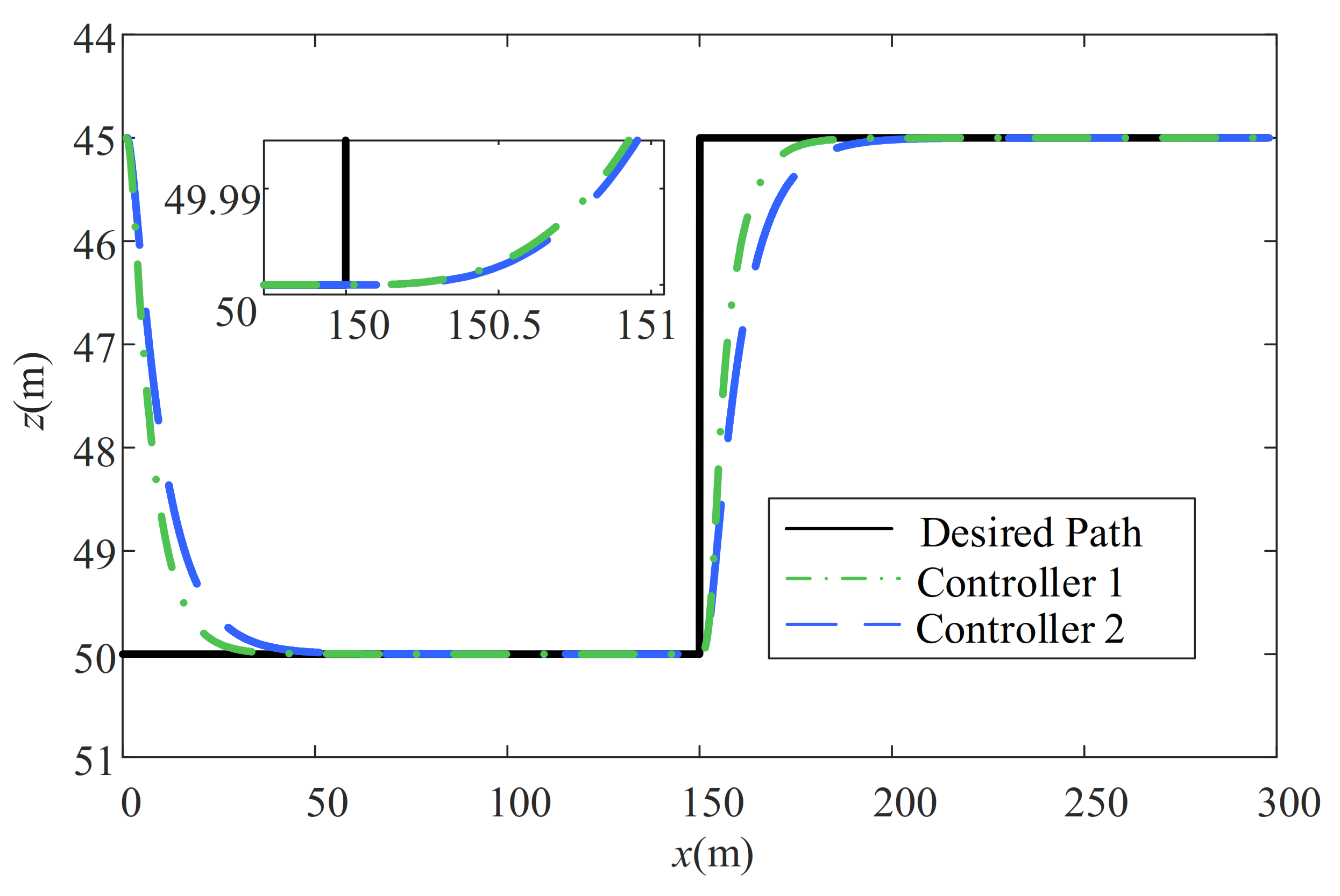
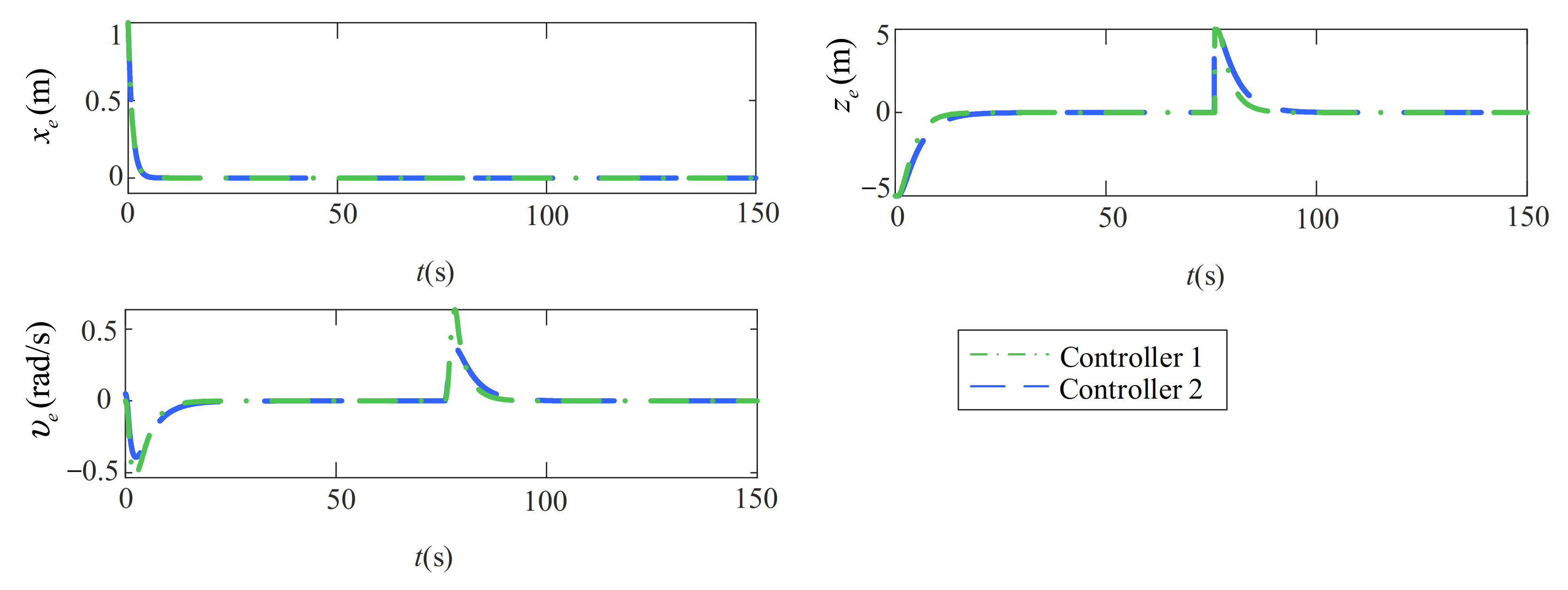
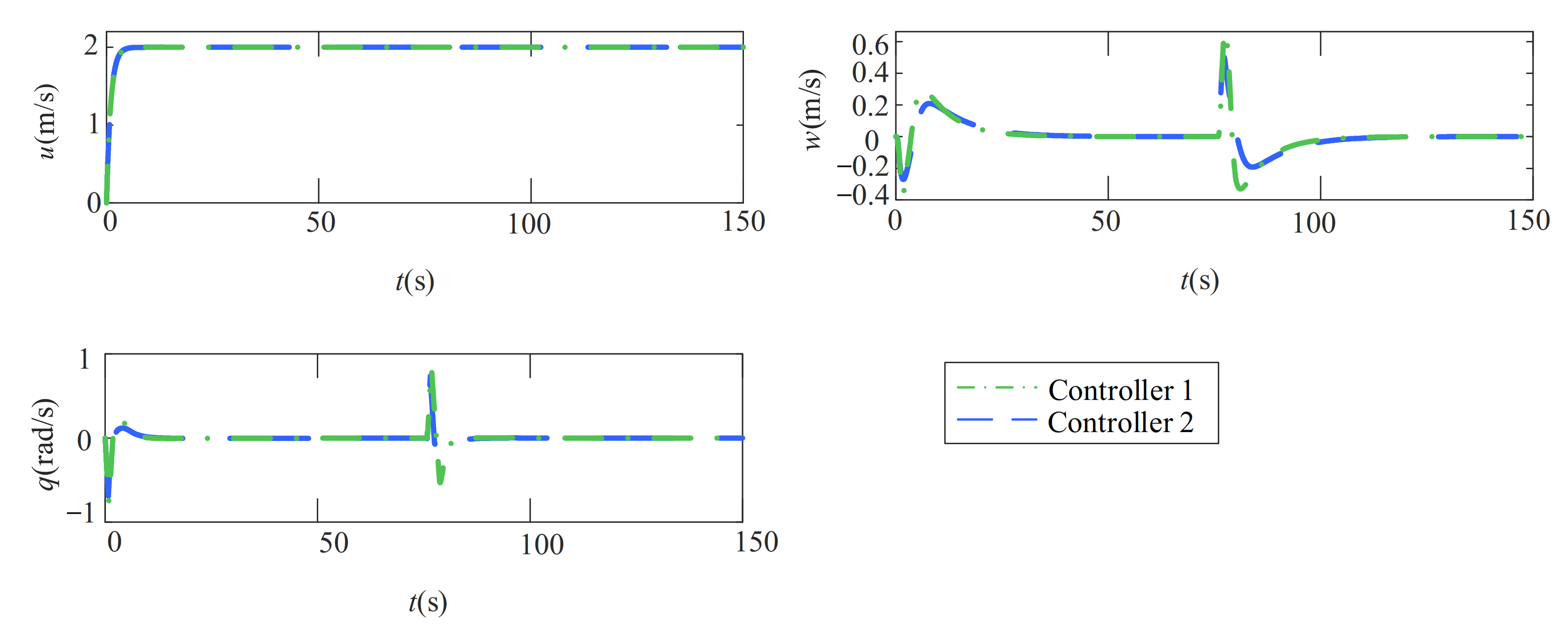
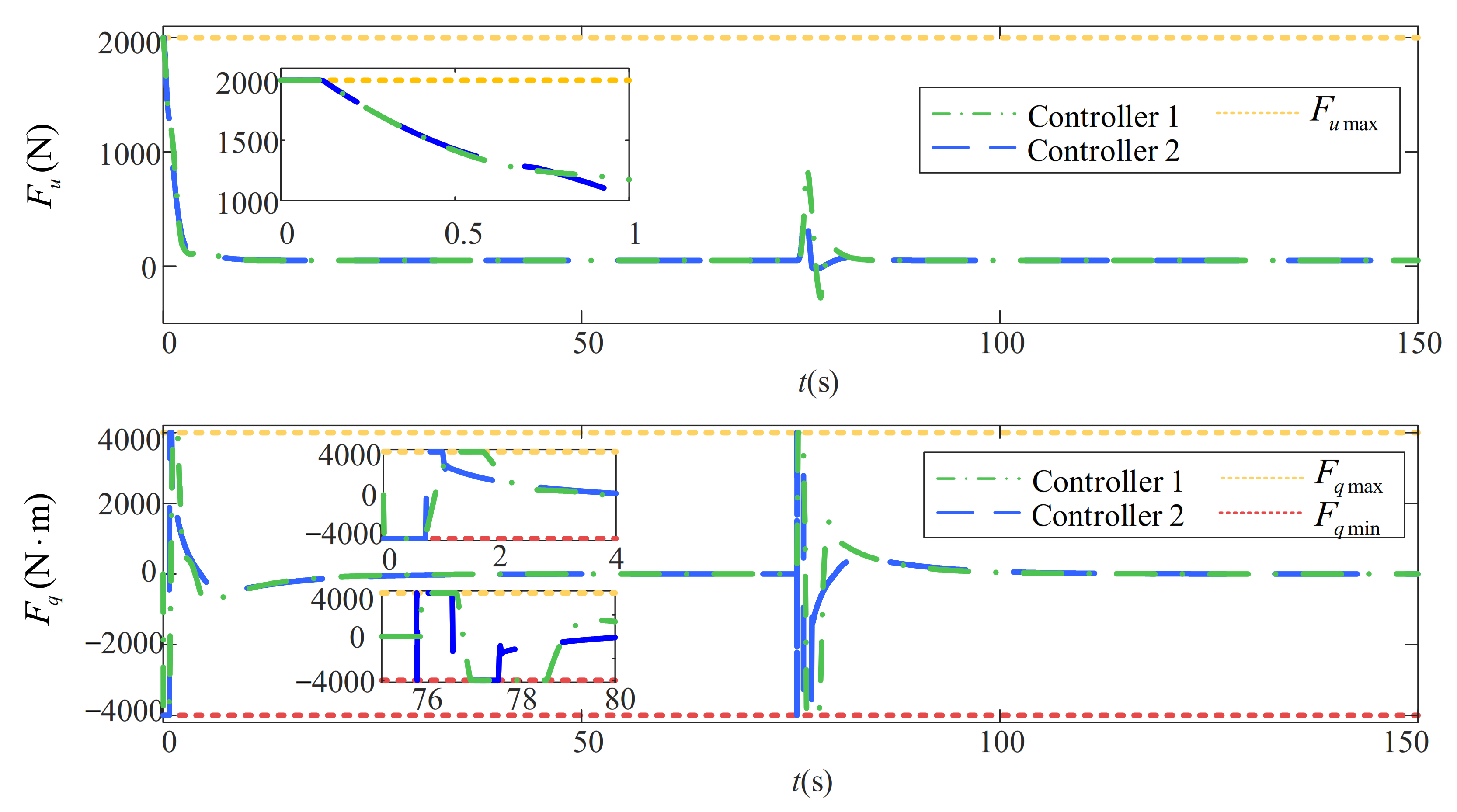
5.1. Comparative Analysis of the Path-Following Performance in the Nominal Working Condition without Disturbances

In the current subsection, the effectiveness of the presented controller is verified through comparison with Controller 2. The initial conditions of the underactuated AUV in the nominal working condition and the designed controller parameters are listed in Table 3. For a fair comparison, the desired path is parameterized as [39]:

$$\left\{\begin{array}{l}{x}_F(\varpi )=\varpi \\ z_F(\varpi )=\left\{\begin{array}{l}50,\varpi \le 150\\ 45,\varpi >150\end{array}\right.\end{array}\right.$$

(33)

where $\varpi (s)$ can be estimated as:

$$\frac{d\varpi }{ds}=\frac{1}{\sqrt{{\left[{\left(x_F\right)}^{\prime }\right]}^2+{\left[{\left(z_F\right)}^{\prime }\right]}^2}}$$

(34)

where ${(x_F)}^{\prime }=\frac{d{x}_F}{d\varpi }$ and ${(z_F)}^{\prime }=\frac{d{z}_F}{d\varpi }$.

Remark 9.

The elevation angle of virtual target point P is ${\upsilon }_F(s)=-{\tan }^{-1}\frac{{(z_F)}^{\prime }}{{(x_F)}^{\prime }}$, and the curvature of the predefined path at the virtual target’s position can be obtained as$c_c(s)=\frac{\partial {\upsilon }_F(s)}{\partial \varpi }\frac{d\varpi }{ds}$.

Table 3. Initial conditions of the underactuated AUV in the nominal working condition and the designed controller parameters.

Initial conditions of the underactuated AUV	$x(0)=1 \mathrm{m}$$,z(0)=45 \mathrm{m}$$,u(0)=0 \mathrm{m}/\mathrm{s}$$,w(0)=0 \mathrm{m}/\mathrm{s}$$,q(0)=0 \mathrm{rad}/\mathrm{s}$$, \theta (0)=0.05 \mathrm{rad}$$,s(0)=0 \mathrm{m}$$,u_d=2 \mathrm{m}/\mathrm{s}$
Controller parameters	$k_1=1$$,k_2=10$$,k_3=1$$,k_4=1$$,{\omega }_1=20$$,{\omega }_2=20$$,{\omega }_3=20$$,{\omega }_4=5$$,h=0.01 {\mathrm{s}}^{-1}$$,r=100 {\mathrm{m}/\mathrm{s}}^2$$,T=0.001 {\mathrm{s}}^{-1}$

Table 3. Initial conditions of the underactuated AUV in the nominal working condition and the designed controller parameters.

Initial conditions of the underactuated AUV	$x(0)=1 \mathrm{m}$$,z(0)=45 \mathrm{m}$$,u(0)=0 \mathrm{m}/\mathrm{s}$$,w(0)=0 \mathrm{m}/\mathrm{s}$$,q(0)=0 \mathrm{rad}/\mathrm{s}$$, \theta (0)=0.05 \mathrm{rad}$$,s(0)=0 \mathrm{m}$$,u_d=2 \mathrm{m}/\mathrm{s}$
Controller parameters	$k_1=1$$,k_2=10$$,k_3=1$$,k_4=1$$,{\omega }_1=20$$,{\omega }_2=20$$,{\omega }_3=20$$,{\omega }_4=5$$,h=0.01 {\mathrm{s}}^{-1}$$,r=100 {\mathrm{m}/\mathrm{s}}^2$$,T=0.001 {\mathrm{s}}^{-1}$

The numerical simulations are presented in Figure 3, Figure 4, Figure 5, Figure 6 and Figure 7. Figure 3 depicts the path-following results of two controllers in the vertical plane. It is evident that both Controller 1 and Controller 2 can drive the underactuated AUV to accurately follow the given path, but Controller 1 has a faster convergence rate than Controller 2. The corresponding path-following errors and speed evolutions are displayed in Figure 4 and Figure 5, respectively. It is easily observed that the path-following errors of two controllers tend to a very narrow band around zero rapidly. Moreover, the surge speed $u$ rapidly converges to the given surge speed $u_d=2 \mathrm{m}/\mathrm{s}$, while the heave and pitch speeds are kept bounded, which is consistent with Theorem 1. However, Controller 1 has a shorter convergent time in position tracking than Controller 2. The control inputs $F_u$ and $F_q$ in the nominal working condition are presented in Figure 6. It can be concluded from Figure 6 that both Controller 1 and Controller 2 can guarantee that the control inputs remain in the boundary range.

According to the above analyses, both Controller 1 and Controller 2 are verified to be effective for path-following in the vertical plane, but Controller 1 exhibits more satisfactory performance than Controller 2 in the nominal working condition.

Figure 3. Path-following results in the nominal working condition.

Figure 3. Path-following results in the nominal working condition.

Figure 4. Path-following errors in the nominal working condition.

Figure 4. Path-following errors in the nominal working condition.

Figure 5. Body-fixed velocities in the nominal working condition.

Figure 5. Body-fixed velocities in the nominal working condition.

Figure 6. Control inputs in the nominal working condition.

Figure 6. Control inputs in the nominal working condition.

Figure 7. Angle of attack and its derivative in the nominal working condition.

Figure 7. Angle of attack and its derivative in the nominal working condition.

5.2. Comparative Analysis of the Path-Following Performance under Multiple Uncertainties

In practical applications, the performance of underactuated AUVs can be affected by external disturbances, perturbations in the internal model parameters, and other unmodeled dynamics. In this subsection, the superiority of Controller 1 under the unknown multiple uncertainties is evaluated through comparison with Controller 3. The initial conditions of the underactuated AUV with multiple uncertainties and the designed controller parameters are presented in Table 4. The multiple uncertainties, which include both internal model parameter perturbations and the external environmental disturbances, are generated as follows [17]:

$$\Delta m_{11}=-0.2m_{11}, \Delta m_{22}=-0.2m_{22}, \Delta m_{33}=-0.1m_{33}, \Delta d_{11}=-0.1d_{11}, \Delta d_{33}=-0.3d_{33}, \Delta L=-0.3L.$$

$$\left\{\begin{array}{l}\Delta F_u=\left(-0.2m_{11}\cos \theta -0.1m_{22}\sin \theta \right)f(t)\\ \Delta F_w=\left(-0.2m_{11}\sin \theta +0.1m_{22}\cos \theta \right)f(t)\\ \Delta F_q=-0.1m_{33}f(t)\end{array}\right.$$

(35)

where $f(t)=1+0.1\sin (2t)$.

For a fair comparison, the desired path is parameterized as [17]:

$$\left\{\begin{array}{l}{x}_F(\varpi )=\varpi \\ z_F(\varpi )=10\left[1+0.25\tanh \left(\frac{\varpi -75}{15}\right)\right]\end{array}\right.$$

(36)

Table 4. Initial conditions of the underactuated AUV with multiple uncertainties and the designed controller parameters.

Initial position and posture of the underactuated AUV	$x(0)=2 \mathrm{m}$$,z(0)=11 \mathrm{m}$$,u(0)=1.5 \mathrm{m}/\mathrm{s}$$,w(0)=0 \mathrm{m}/\mathrm{s}$$,q(0)=0 \mathrm{rad}/\mathrm{s}$$, \theta (0)=0 \mathrm{rad}$$,s(0)=0 \mathrm{m}$$,u_d=2 \mathrm{m}/\mathrm{s}$
Controller parameters	$k_1=5$$,k_2=5$$,k_3=1$$,k_4=1$$,{\omega }_1=20$$,{\omega }_2=20$$,{\omega }_3=20$$,{\omega }_4=0.5$$,h=0.01 {\mathrm{s}}^{-1}$$,r=100 {\mathrm{m}/\mathrm{s}}^2$$,T=0.001 {\mathrm{s}}^{-1}$

Table 4. Initial conditions of the underactuated AUV with multiple uncertainties and the designed controller parameters.

Initial position and posture of the underactuated AUV	$x(0)=2 \mathrm{m}$$,z(0)=11 \mathrm{m}$$,u(0)=1.5 \mathrm{m}/\mathrm{s}$$,w(0)=0 \mathrm{m}/\mathrm{s}$$,q(0)=0 \mathrm{rad}/\mathrm{s}$$, \theta (0)=0 \mathrm{rad}$$,s(0)=0 \mathrm{m}$$,u_d=2 \mathrm{m}/\mathrm{s}$
Controller parameters	$k_1=5$$,k_2=5$$,k_3=1$$,k_4=1$$,{\omega }_1=20$$,{\omega }_2=20$$,{\omega }_3=20$$,{\omega }_4=0.5$$,h=0.01 {\mathrm{s}}^{-1}$$,r=100 {\mathrm{m}/\mathrm{s}}^2$$,T=0.001 {\mathrm{s}}^{-1}$

The simulation results are shown in Figure 8, Figure 9, Figure 10, Figure 11, Figure 12 and Figure 13. From Figure 8, it is easily observed that both Controller 1 and Controller 3 can regulate the underactuated AUV to accurately follow the predefined path. The path-following performance is presented in Figure 9 and Figure 10. It is evident that the path-following errors of two controllers converge to the vicinity of zero, but Controller 1 has superior path-following accuracy and smaller steady-state error than Controller 3. The reason is that Controller 1 has a faster convergence rate than Controller 3. From Figure 11, it is evident that the control inputs of Controller 3 violate the input constraints during the transient phase, whereas Controller 1 can limit the control inputs into a valid range. Figure 12 shows the estimated and actual values of the kinematic uncertainty and the dynamic uncertainties, which demonstrates that the kinematic and dynamic uncertainties can be accurately and rapidly estimated by the designed reduced-order ESOs, respectively. The desired pitch speed $q_d$ and the outputs ($q_c$ and ${\dot{q}}_c$) obtained by NTD are shown in Figure 14. It is evident that the output $q_c$ generated by NTD rapidly tracks the desired pitch speed $q_d$.

The above simulation results and analyses indicate the superiority of Controller 1 compared with Controller 3. Controller 1 provides improved performance under the given multiple uncertainties. This improved performance is attributed to the precise estimation of the kinematic and dynamic uncertainties in real time.

Figure 8. Path-following results under multiple uncertainties.

Figure 8. Path-following results under multiple uncertainties.

Figure 9. Path-following errors under multiple uncertainties.

Figure 9. Path-following errors under multiple uncertainties.

Figure 10. Body-fixed velocities under multiple uncertainties.

Figure 10. Body-fixed velocities under multiple uncertainties.

Figure 11. Control inputs under multiple uncertainties.

Figure 11. Control inputs under multiple uncertainties.

Figure 12. The estimated and actual values of the kinematic and dynamic uncertainties.

Figure 12. The estimated and actual values of the kinematic and dynamic uncertainties.

Figure 13. Desired pitch speed $q_d$ and the outputs ($q_c$ and ${\dot{q}}_c$) produced by NTD under multiple uncertainties.

Figure 13. Desired pitch speed $q_d$ and the outputs ($q_c$ and ${\dot{q}}_c$) produced by NTD under multiple uncertainties.

Figure 14. Path-following results in both cases.

Figure 14. Path-following results in both cases.

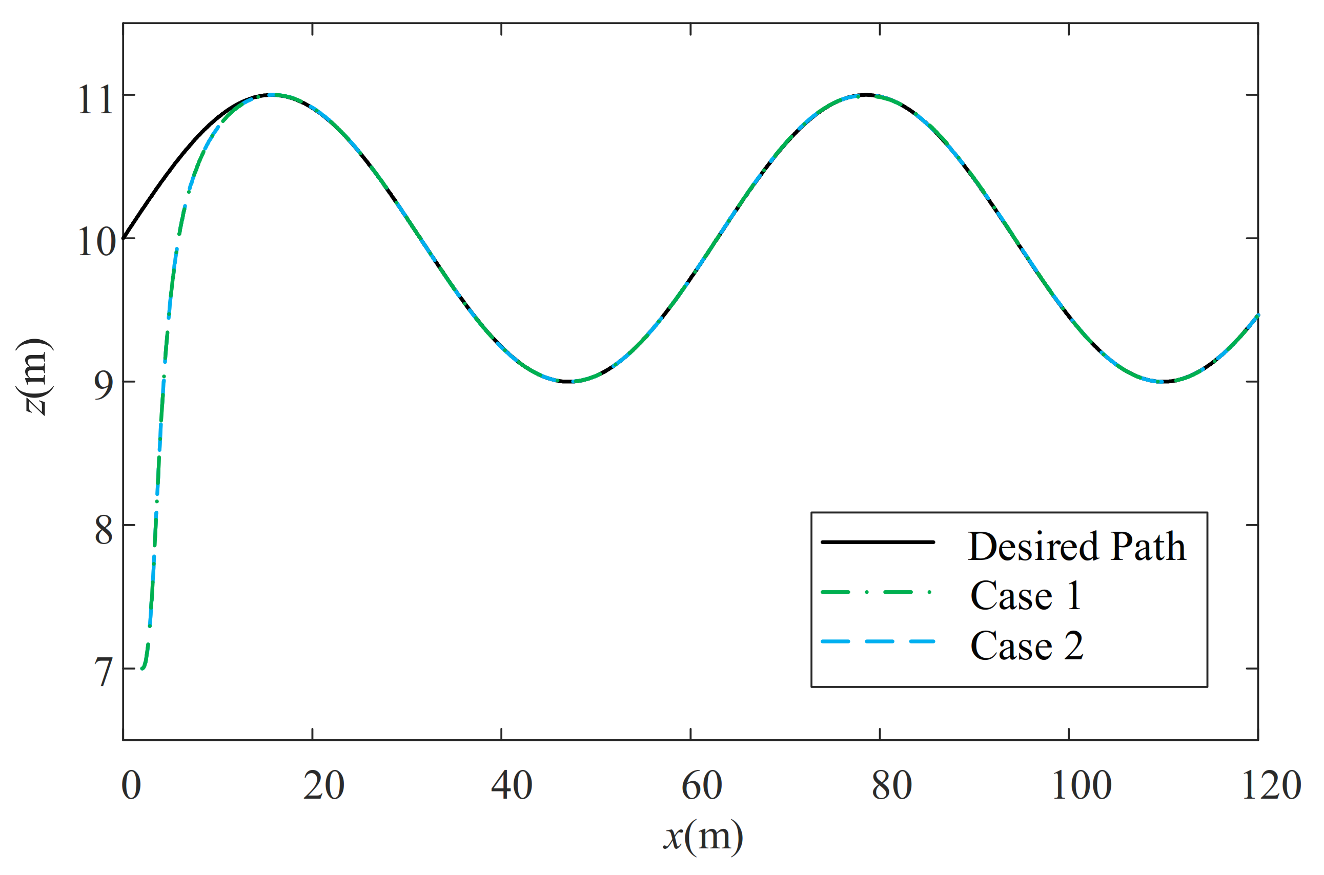
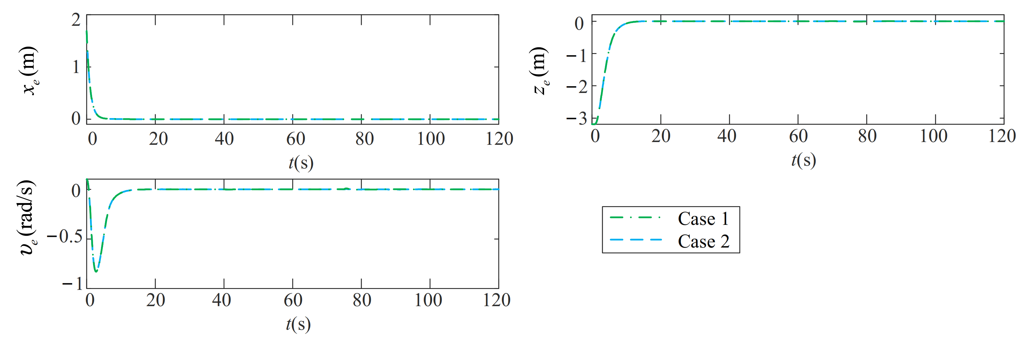
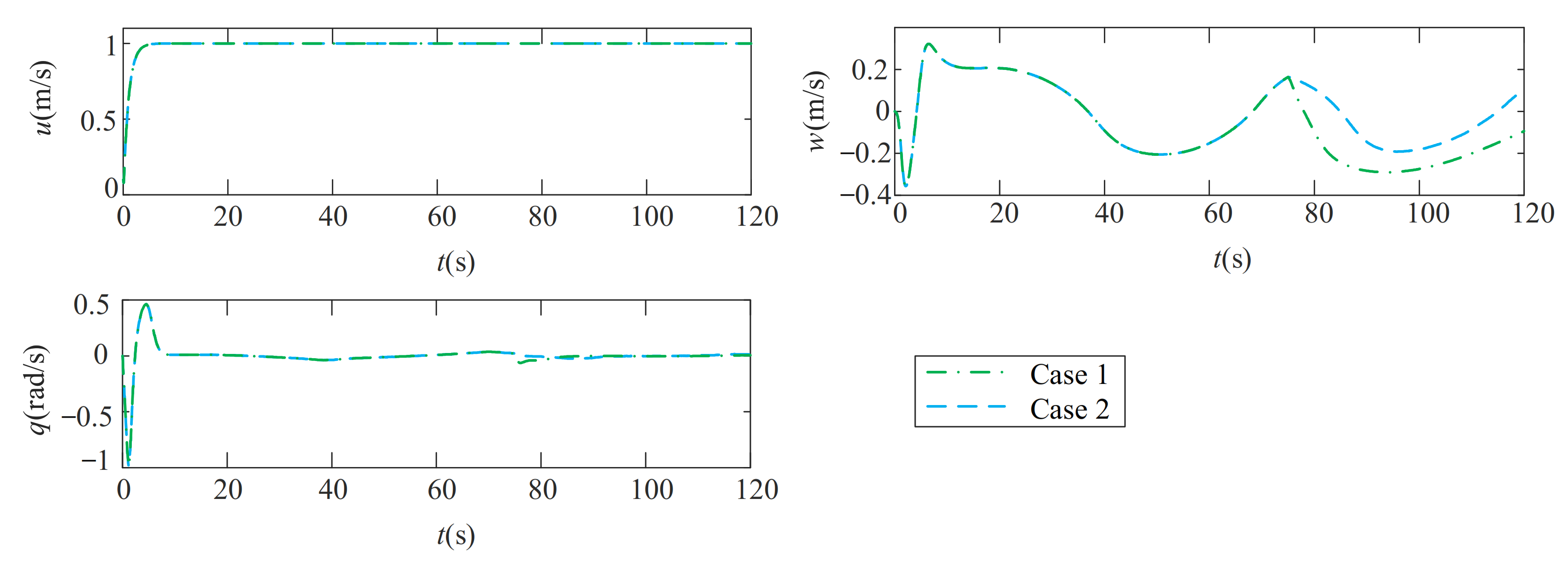
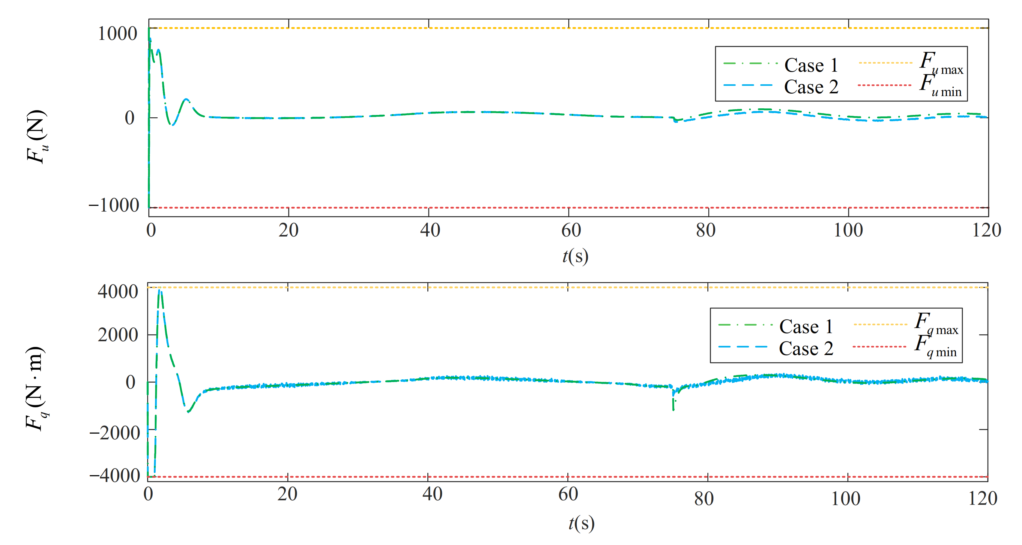
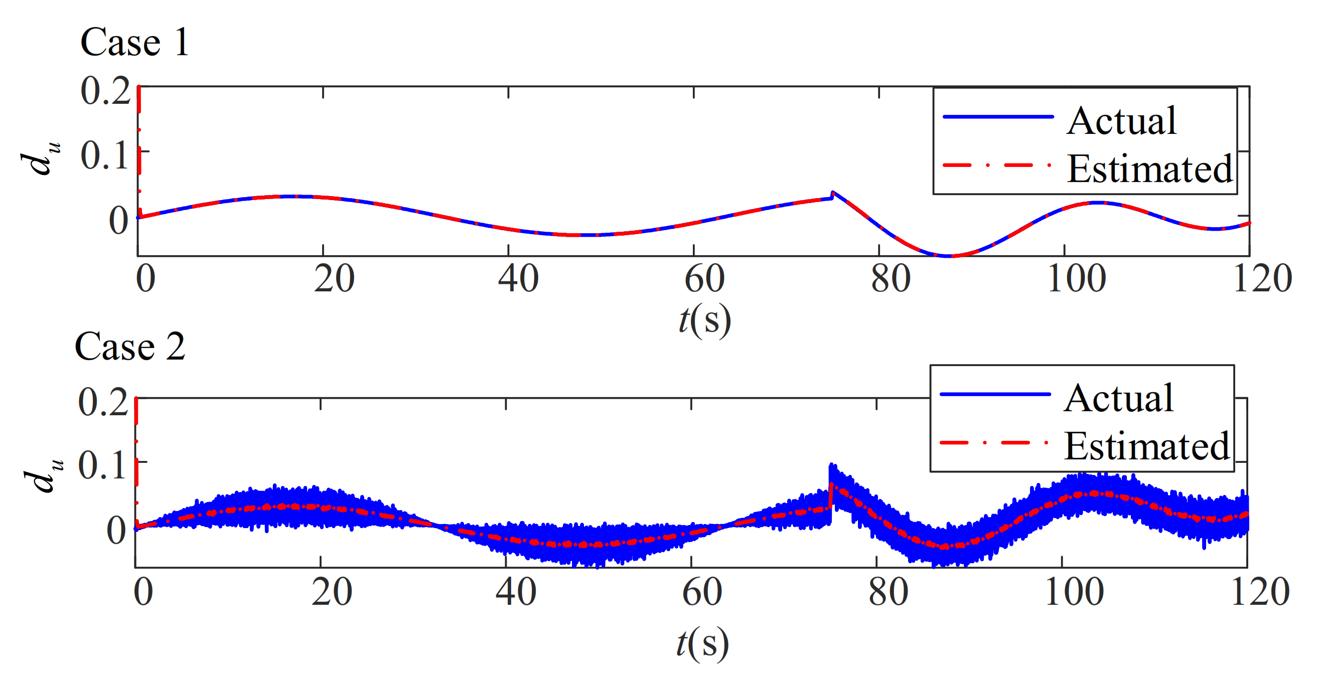
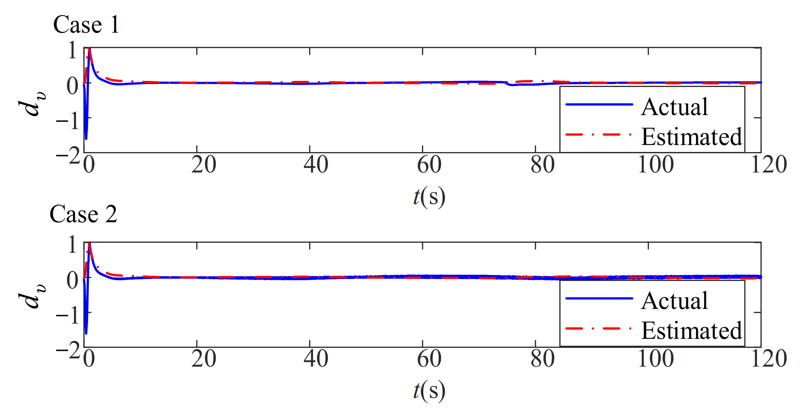
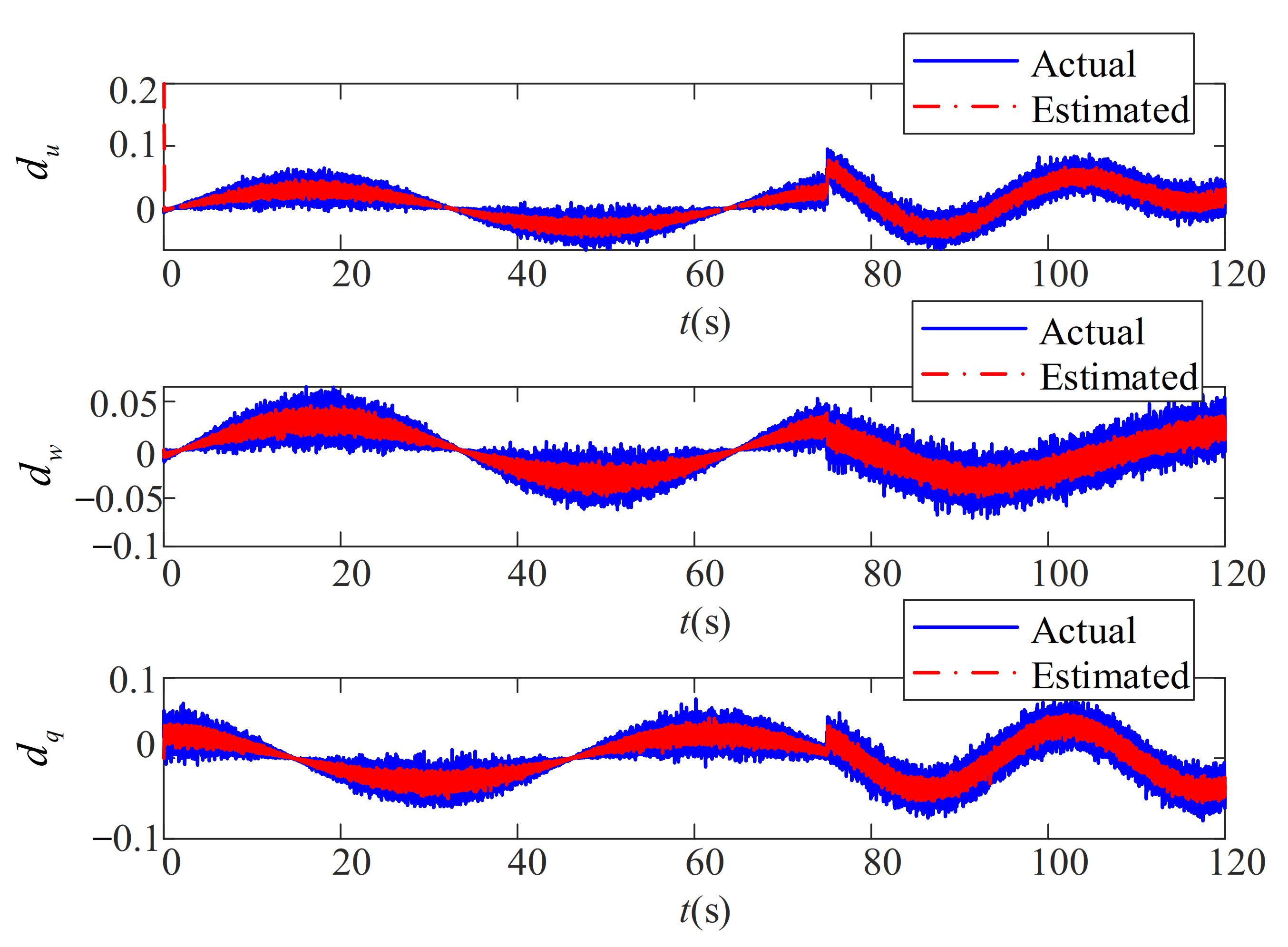
5.3. Robustness Analysis for the Path-Following Performance in the Conditions Which Better Replicate the Actual Environment

To evaluate whether Controller 1 can operate well in the actual working environment, in this subsection, two different kinds of disturbances which better replicate the actual environment, including complex segmented disturbances and more complex segmented disturbances with high-frequency noise, are introduced to the control system, respectively. The specific dynamic uncertainties are generated as follows [41]:

Case 1:

$$\left\{\begin{array}{l}{d}_u=\left\{\begin{array}{l}0.03\sin (0.1t-0.1)t<75s\\ 0.03u\cos (0.1t)+0.04\sin (0.2t)+0.03u^2-0.03t\ge 75s\end{array}\right.\\ d_w=\left\{\begin{array}{l}0.03\sin (0.1t-0.2)t<75s\\ 0.04w\sin (0.1t)+0.03\cos (0.1t)-0.03w^2-0.03t\ge 75s\end{array}\right.\\ d_q=\left\{\begin{array}{l}0.03\cos (0.1t+0.1)t<75s\\ 0.03q\cos (0.1t)+0.04\sin (0.2t)-0.03q^2+0.03t\ge 75s\end{array}\right.\end{array}\right.$$

Case 2:

$$\left\{\begin{array}{l}{d}_u=\left\{\begin{array}{l}(0.03+\mathrm{normrnd}(0,0.01))\sin (0.1t-0.1+\mathrm{normrnd}(0,0.01))t<75s\\ 0.03u\cos (0.1t)+0.04\sin (0.2t)+0.03u^2-\mathrm{normrnd}(0,0.01) t\ge 75s\end{array}\right.\\ d_w=\left\{\begin{array}{l}(0.03+\mathrm{normrnd}(0,0.01\left)\right)\sin (0.1t-0.2+\mathrm{normrnd}(0,0.01))t<75s\\ 0.04w\sin (0.1t)+0.03\cos (0.1t)-0.03w^2-\mathrm{normrnd}(0,0.01) t\ge 75s\end{array}\right.\\ d_q=\left\{\begin{array}{l}(0.03+\mathrm{normrnd}(0,0.01\left)\right)\cos (0.1t+0.1+\mathrm{normrnd}(0,0.01))t<75s\\ 0.03q\cos (0.1t)+0.04\sin (0.2t)-0.03q^2+\mathrm{normrnd}(0,0.01) t\ge 75s\end{array}\right.\end{array}\right.$$

The desired path is given as [41]:

$$\left\{\begin{array}{l}{x}_F(\varpi )=\varpi \\ z_F(\varpi )=10+\sin (0.1\varpi )\end{array}\right.$$

The simulation results are shown in Figure 14, Figure 15, Figure 16, Figure 17, Figure 18, Figure 19, Figure 20 and Figure 21. Figure 15 and Figure 16 depict the path-following results and their corresponding path-following errors, respectively. It is evident that even for more complicated path and more actual environmental disturbances, Controller 1 still effectively forces the AUV to follow the desired path, and all path-following errors still quickly tend to narrow bound fields near the origin. Since the kinematic and dynamic uncertainties are compensated via reduced-order ESOs in time, the steady-state tracking errors of Controller 1 are maintained at a low level in the two different kinds of disturbances. As shown in Figure 16, the surge speed can accurately and rapidly converge to the given speed. The input force and torque are presented in Figure 18. Small fluctuations occur in the control inputs as the dynamic uncertainties with random noise are continuously and abruptly varied in Case 2, which is reasonable because the input force and torque need some time to adjust.

The estimated values of $d_u$, $d_w$, $d_q$, and $d_{\upsilon }$ are shown in Figure 18, Figure 19, Figure 20 and Figure 21. The dynamic and kinematic uncertainties can be accurately estimated for a system with complex segmented disturbances in Case 1 using the designed reduced-order ESOs in time. Moreover, although the dynamic uncertainties with random noise are continuously and suddenly changed, only a slight chattering can be observed in the estimation of $d_u$, $d_w$, and $d_q$ in Case 2, which is acceptable in complex sea conditions.

Remark 10.

According to the above results and analyses, the proposed controller in this paper provides satisfactory performance and enhanced robustness in the above two kinds of disturbances due to the timely and accurate observability of the established reduced-order ESOs. As shown in Figure 22, it is noted that with the increase in the bandwidth of the observer, the estimation accuracy of the observer is improved, but it also becomes more sensitive to high-frequency noise. In reality, satisfactory performance in the presence of random noise can be attained by adjusting the observer bandwidth to make a tradeoff between the estimation precision and the sensitivity to noise.

Figure 15. Path-following errors in both cases.

Figure 15. Path-following errors in both cases.

Figure 16. Body-fixed velocities in both cases.

Figure 16. Body-fixed velocities in both cases.

Figure 17. Control inputs in both cases.

Figure 17. Control inputs in both cases.

Figure 18. Estimate and actual of $d_u$ in both cases.

Figure 18. Estimate and actual of $d_u$ in both cases.

Figure 19. Estimate and actual of $d_w$ in both cases.

Figure 19. Estimate and actual of $d_w$ in both cases.

Figure 20. Estimate and actual of $d_q$ in both cases.

Figure 20. Estimate and actual of $d_q$ in both cases.

Figure 21. Estimate and actual of $d_{\upsilon }$ in both cases.

Figure 21. Estimate and actual of $d_{\upsilon }$ in both cases.

Figure 22. Estimates and actual of $d_u$, $d_w$, and $d_q$ in larger bandwidth (${\omega }_1=500$, ${\omega }_2=500$, ${\omega }_3=500$).

Figure 22. Estimates and actual of $d_u$, $d_w$, and $d_q$ in larger bandwidth (${\omega }_1=500$, ${\omega }_2=500$, ${\omega }_3=500$).

6. Conclusions

This paper presents a novel augmented back-stepping controller to solve the path-following issue of an underactuated AUV with multiple uncertainties. Reduced-order ESOs and NTD are employed to construct an augmented back-stepping controller. Four reduced-order ESOs are designed to estimate the kinematic and dynamic uncertainties, and an NTD is adopted to minimize the impact of the input saturation issue and overcome the problem of “explosion of complexity” associated with traditional back-stepping method. A stability analysis of the proposed controller is established through the Lyapunov theorem to guarantee that the tracking errors uniformly tend to a narrow bound near zero. Extensive simulations and robustness analyses are performed to verify the efficiency, superiority, and robustness of the presented controller. It should be pointed out that due to the complexity of the experiment setup and cost limitations, experimental verification is not carried out in this paper. In future work, observers and stochastic control methods will be combined further to improve the controller performance subject to disturbances with random noises. We will extend the proposed path-following controller to the motion in 3-D space.

References

1. Xiang, X.; Yu, C.; Zhang, Q. Robust fuzzy 3D path following for autonomous underwater vehicle subject to uncertainties. Comput. Oper. Res. 2017, 84, 165–177. [Google Scholar] [CrossRef]
2. Peng, Z.; Wang, J.; Wang, J. Constrained control of autonomous underwater vehicles based on command optimization and disturbance estimation. IEEE Trans. Ind. Electron. 2018, 66, 3627–3635. [Google Scholar] [CrossRef]
3. Wang, H.; Li, Y.; Liu, K. Globally stable adaptive dynamic surface control for cooperative path following of multiple underactuated autonomous underwater vehicles. Asian J. Control 2018, 20, 1204–1220. [Google Scholar] [CrossRef]
4. Duan, K.; Fong, S.; Chen, C.P. Multilayer neural networks-based control of underwater vehicles with uncertain dynamics and disturbances. Nonlinear Dyn. 2020, 100, 3555–3573. [Google Scholar] [CrossRef]
5. Fan, S.; Chan, K.; Chin, C. Motion Analysis of an Autonomous Underwater Vehicle Tethered with an Optical Fiber for Real-Time Surveillance. IEEE J. Ocean. Eng. 2020, 46, 434–446. [Google Scholar] [CrossRef]
6. Yu, C.; Xiang, X.; Lapierre, L.; Zhang, Q. Nonlinear guidance and fuzzy control for three-dimensional path following of an underactuated autonomous underwater vehicle. Ocean Eng. 2017, 146, 457–467. [Google Scholar] [CrossRef] [Green Version]
7. Shen, C.; Shi, Y.; Buckham, B. Path-following control of an AUV: A multiobjective model predictive control approach. IEEE Trans. Control Syst. Technol. 2018, 27, 1334–1342. [Google Scholar] [CrossRef]
8. Fossen, T.I. Handbook of Marine Craft Hydrodynamics and Motion Control; John Wiley & Sons: Hoboken, NJ, USA, 2011. [Google Scholar]
9. Zheng, Z.; Sun, L.; Xie, L. Error-constrained LOS path following of a surface vessel with actuator saturation and faults. IEEE Trans. Syst. Man Cybern. Syst. 2017, 48, 1794–1805. [Google Scholar] [CrossRef]
10. Wichlund, K.; Sordalen, O.; Egeland, O. Control properties of underactuated vehicles. In Proceedings of the 1995 IEEE International Conference on Robotics and Automation, Nagoya, Japan, 21–27 May 1995; pp. 2009–2014. [Google Scholar]
11. Xiang, X.; Yu, C.; Zhang, Q.; Xu, G. Path-following control of an auv: Fully actuated versus under-actuated configuration. Mar. Technol. Soc. J. 2016, 50, 34–47. [Google Scholar] [CrossRef]
12. He, S.; Dai, S.-L.; Luo, F. Asymptotic trajectory tracking control with guaranteed transient behavior for MSV with uncertain dynamics and external disturbances. IEEE Trans. Ind. Electron. 2018, 66, 3712–3720. [Google Scholar] [CrossRef]
13. Cho, G.R.; Li, J.H.; Park, D.; Jung, J.H. Robust trajectory tracking of autonomous underwater vehicles using back-stepping control and time delay estimation. Ocean Eng. 2020, 201, 107131. [Google Scholar] [CrossRef]
14. Xia, G.; Xia, X.; Sun, X. Formation control with collision avoidance for underactuated surface vehicles. Asian J. Control 2021. [Google Scholar] [CrossRef]
15. Yan, S. Sliding mode tracking control of autonomous underwater vehicles with the effect of quantization. Ocean Eng. 2018, 151, 322–328. [Google Scholar] [CrossRef]
16. Yan, Z.; Wang, M.; Xu, J. Robust adaptive sliding mode control of underactuated autonomous underwater vehicles with uncertain dynamics. Ocean Eng. 2019, 173, 802–809. [Google Scholar] [CrossRef]
17. Yu, C.; Xiang, X.; Zuo, M.; Xu, G. Robust variable-depth path following of an under-actuated autonomous underwater vehicle with uncertainties. Ind. J. Geo-Mar. Sci. 2017, 46, 2543–2551. [Google Scholar]
18. Seok Park, B. Neural network-based tracking control of underactuated autonomous underwater vehicles with model uncertainties. J. Dyn. Syst. Meas. Control 2015, 137, 184–204. [Google Scholar] [CrossRef]
19. Yan, Z.; Wang, M.; Xu, J. Global adaptive neural network control of underactuated autonomous underwater vehicles with parametric modeling uncertainty. Asian J. Control 2019, 21, 1342–1354. [Google Scholar] [CrossRef]
20. Liang, X.; Qu, X.; Hou, Y.; Li, Y.; Zhang, R. Finite-time unknown observer based coordinated path-following control of unmanned underwater vehicles. J. Frankl. Inst. 2021, 358, 2703–2721. [Google Scholar] [CrossRef]
21. Kim, E.; Fan, S.; Bose, N.; Nguyen, H. Current Estimation and Path Following for an Autonomous Underwater Vehicle (AUV) by Using a High-gain Observer Based on an AUV Dynamic Model. Int. J. Control Autom. Syst. 2020, 19, 478–490. [Google Scholar] [CrossRef]
22. Zhang, Y.; Liu, X.; Luo, M.; Yang, C. MPC-based 3-D trajectory tracking for an autonomous underwater vehicle with constraints in complex ocean environments. Ocean Eng. 2019, 189, 106309. [Google Scholar] [CrossRef]
23. Gonzalez-Garcia, A.; Castañeda, H. Guidance and Control Based on Adaptive Sliding Mode Strategy for a USV Subject to Uncertainties. IEEE J. Ocean. Eng. 2021, 46, 1144–1154. [Google Scholar] [CrossRef]
24. Zhang, J.; Xiang, X.; Lapierre, L.; Zhang, Q.; Li, W. Approach-angle-based three-dimensional indirect adaptive fuzzy path following of under-actuated AUV with input saturation. Appl. Ocean Res. 2021, 107, 102486. [Google Scholar] [CrossRef]
25. Aguiar, A.P.; Hespanha, J.P. Trajectory-tracking and path-following of underactuated autonomous vehicles with parametric modeling uncertainty. IEEE Trans. Autom. Control 2007, 52, 1362–1379. [Google Scholar] [CrossRef] [Green Version]
26. Lapierre, L.; Jouvencel, B. Robust nonlinear path-following control of an AUV. IEEE J. Ocean. Eng. 2008, 33, 89–102. [Google Scholar] [CrossRef]
27. Do, K.D.; Pan, J.; Jiang, Z.-P. Robust and adaptive path following for underactuated autonomous underwater vehicles. Ocean Eng. 2004, 31, 1967–1997. [Google Scholar] [CrossRef]
28. Liao, Y.-l.; Wan, L.; Zhuang, J.-Y. Backstepping dynamical sliding mode control method for the path following of the underactuated surface vessel. Procedia Eng. 2011, 15, 256–263. [Google Scholar] [CrossRef] [Green Version]
29. Han, J. From PID to active disturbance rejection control. IEEE Trans. Ind. Electron. 2009, 56, 900–906. [Google Scholar] [CrossRef]
30. Huang, Y.; Xue, W. Active disturbance rejection control: Methodology and theoretical analysis. ISA Trans. 2014, 53, 963–976. [Google Scholar] [CrossRef]
31. Chen, W.-H.; Yang, J.; Guo, L.; Li, S. Disturbance-observer-based control and related methods—An overview. IEEE Trans. Ind. Electron. 2015, 63, 1083–1095. [Google Scholar] [CrossRef] [Green Version]
32. Lu, L.; Dan, W.; Peng, Z. ESO-Based Line-of-Sight Guidance Law for Path Following of Underactuated Marine Surface Vehicles with Exact Sideslip Compensation. IEEE J. Ocean. Eng. 2017, 42, 477–487. [Google Scholar] [CrossRef]
33. Peng, Z.; Wang, J.; Han, Q.-L. Path-following control of autonomous underwater vehicles subject to velocity and input constraints via neurodynamic optimization. IEEE Trans. Ind. Electron. 2018, 66, 8724–8732. [Google Scholar] [CrossRef]
34. Zhang, Y.; Wang, X.; Wang, S.; Miao, J. DO-LPV-based robust 3D path following control of underactuated autonomous underwater vehicle with multiple uncertainties. ISA Trans. 2020, 101, 189–203. [Google Scholar] [CrossRef]
35. Xu, H.; Zhang, G.C.; Cao, J.; Pang, S.; Sun, Y.S. Underactuated AUV Nonlinear Finite-Time Tracking Control Based on Command Filter and Disturbance Observer. Sensors 2019, 19, 4987. [Google Scholar] [CrossRef] [Green Version]
36. Subudhi, B.; Mukherjee, K.; Ghosh, S. A static output feedback control design for path following of autonomous underwater vehicle in vertical plane. Ocean Eng. 2013, 63, 72–76. [Google Scholar] [CrossRef]
37. Mahapata, S.; Subudhi, B. Design of a steering control law for an autonomous underwater vehicle using nonlinear H state feedback technique. Nonlinear Dyn. 2017, 90, 837–854. [Google Scholar] [CrossRef]
38. Guo, C.; Han, Y.; Yu, H.; Qin, J. Spatial path-following control of underactuated auv with multiple uncertainties and input saturation. IEEE Access 2019, 7, 98014–98022. [Google Scholar] [CrossRef]
39. Yu, C.; Xiang, X. Vertical plane path following control of an under-actuated autonomous underwater vehicle. In Proceedings of the 2016 IEEE International Conference on Underwater System Technology: Theory and Applications (USYS), Penang, Malaysia, 13–14 December 2016. [Google Scholar]
40. Miao, J.; Wang, S.; Zhao, Z.; Li, Y.; Tomovic, M.M. Spatial curvilinear path following control of underactuated AUV with multiple uncertainties. ISA Trans. 2017, 67, 107–130. [Google Scholar] [CrossRef]
41. Xia, Y.; Xu, K.; Wang, W.; Xu, G.; Xiang, X.; Li, Y. Optimal robust trajectory tracking control of a X-rudder AUV with velocity sensor failures and uncertainties. Ocean Eng. 2020, 198, 106949. [Google Scholar] [CrossRef]
42. Xingling, S.; Honglun, W. Back-stepping active disturbance rejection control design for integrated missile guidance and control system via reduced-order ESO. ISA Trans. 2015, 57, 10–22. [Google Scholar] [CrossRef]
43. Shao, X.; Wang, H. Active disturbance rejection based trajectory linearization control for hypersonic reentry vehicle with bounded uncertainties. ISA Trans. 2015, 54, 27–38. [Google Scholar] [CrossRef]
44. Lapierre, L.; Soetanto, D. Nonlinear path-following control of an AUV. Ocean Eng. 2007, 34, 1734–1744. [Google Scholar] [CrossRef]
45. Arnold, V. Mathematical Method of Classic Mechanics; Springer: New York, NY, USA, 1988. [Google Scholar]
46. Khalil, H.K.; Grizzle, J.W. Nonlinear Systems; Prentice Hall: Upper Saddle River, NJ, USA, 2002; Volume 3. [Google Scholar]
47. Do, K.D.; Pan, J. Control of Ships and Underwater Vehicles: Design for Underactuated and Nonlinear Marine Systems; Springer Science & Business Media: Boston, MA, USA, 2009. [Google Scholar]
48. McEwen, R.; Streitlien, K. Modeling and control of a variable-length auv. In Proceedings of the 12th International Symposium on Unmanned Untethered Submersible Technology, Durham, NH, USA, 27 August 2001. [Google Scholar]
Figure 1. The geometric description of vertical path following of an underactuated AUV.
Jmse 10 00238 g001
Figure 2. The presented control structure for the underactuated AUV.
Jmse 10 00238 g002