Fluid–Structure Interaction Analysis and Verification Test for Soil Penetration to Determine the Burial Depth of Subsea HVDC Cable

Abstract

Recently, there have been frequent reports of subsea cable breakage accidents caused by the drop of an anchor pile for aquaculture works involving subsea cables for high-voltage direct current (HVDC) transmission embedded in the southwest sea of Korea. To determine the burial depth that can ensure the safety of subsea HVDC cables embedded under the seabed from the drop of anchor files, the soil penetration characteristics of anchor piles should be reasonably estimated. In the present study, the penetration characteristics of anchor piles into the soil under which subsea HVDC cables are embedded were evaluated using numerical simulations and field verification tests. The numerical simulation for the soil penetration phenomena of anchor piles was carried out using the fluid–structure interaction analysis method using the general purpose nonlinear finite element analysis code based on explicit time integration. Regarding the soil into which anchor piles penetrate, three types of soil—a clay layer, a sand layer, and a clay–sand mixed layer—were considered, which are the representative soil types in the southwest sea of Korea, where many subsea HVDC cables have been embedded. The result of fluid–structure interaction analysis showed that the maximum penetration into the clay layer was higher than that into the sand layer and the clay–sand mixed layer by 86.3% and 36.4% or more, respectively. The error rates of the field verification test and the fluid–structure interaction analysis were found to be 9.8%, 2.4%, and 2.4% in the clay layer, the sand layer, and the clay–sand mixed layer, respectively, which were found to be reasonable levels when considering that it was the numerical simulation for the soil penetration of an anchor pile resulting from drop impacts. The penetration depths of anchor piles were found to be the deepest in the clay layer, showing values of 3.9 to 4.1 m, and those in the sand layer were the shallowest, showing values of 1.9 to 2.1 m.

1. Introduction

Subsea cables are used not only for the large-scale transmission/distribution of electric power between land and islands and between neighboring countries but also as a major infrastructure for overseas intelligence communication in place of satellite communication. The installation of subsea cable is experiencing a globally increasing trend, and breakage accidents are also showing increasing trend as a result [1]. It is reported that the main causes of subsea cable breakage accidents are anchor collisions caused by the anchoring and dragging of anchors for ships and impact damage caused by the soil penetration of anchor piles used during offshore aquaculture works [2]. Recently, frequent reports have been made of subsea cable breakage accidents caused by the drop of an anchor pile on subsea cables for high-voltage direct current (HVDC) transmission embedded in the southwest sea of Korea [2,3]. Since the social and economic costs required for the restoration are high when a subsea HVDC cable breakage accident occurs, various protection methods have been applied, depending on the characteristics of the seabed ground under which subsea HVDC cables are embedded. In the sea areas where the seabed is formed mostly with clay, sand, or clay–sand mixed soil, a protection method of burying the subsea HVDC cable at a certain depth is applied, and in the sea areas where the seabed is formed with bed rocks or hard soil, a method of bottoming a protective structure in the form of a duct, mattress, or rock-burm onto the upper part of the subsea HVDC cable is applied [4]. In the meantime, since no international regulation or standard on the protection method of subsea HVDC cables or the design of protective structures has been presented, a numerical simulation or test and evaluation method is required to be developed, taking into account the actual environmental conditions in order to ensure the installation safety of subsea HVDC cables. In the case of a buried cable protection method in particular, there is a great need to establish a reasonable evaluation method because the construction sea area is wide and the risk of damage due to the soil penetration of a hazardous element such as an anchor pile is very high.

A number of studies have been conducted in relation to the performance evaluation based on a numerical simulation and test method of soil penetration. Foster Jr. et al. carried out a soil penetration simulation of a standard conical specimen for clay and sandy soil using a general purpose finite element analysis program to develop a soil model for numerical analysis and compared the result with experimental results [5]. Choi et al. conducted a test study to minimize the measurement deviation of repulsion and final penetration during the soil penetration of a pile [6]. Kim et al. carried out a numerical simulation using a general purpose finite element analysis program to estimate the ultimate bearing capacity generated during the sandy soil penetration of a suction anchor for a marine structure and to determine the loading position where the maximum bearing capacity can be expressed [7]. Kim and Jeong carried out a numerical simulation using the Coupled Eulerian-Lagrangian (CEL) method to predict the soil penetration characteristics of a torpedo anchor used for the foundation of a deep-sea floating structure [8]. Grabe et al. carried out a numerical simulation using the CEL method to numerically simulate the sandy soil penetration test result of an anchor for ship [9]. Go et al. carried out a large deformation analysis using the CEL technique to directly simulate the soil penetration process of a driven pile and compared the modeling technique and analysis result with the field test result [10]. Shin et al. carried out a numerical analysis study, considering the contact condition and geostatic stress, to estimate the ice keel gouging depth required for the design of an arctic pipeline system [11]. Moore et al. proposed a design guidance of the cable burial depths given in relation to anchor size, anchor mass, and ship mass using test results of miniature anchor that was dragged through sand of different densities within a centrifuge [12]. Robinson et al. investigated the factors controlling the plough resistance using a series of dry and saturated scale model cable plough tests in sand in a geotechnical centrifuge at a range of target trench depths, sand relative densities, and plough velocities [13]. Zheng et al. conducted physical model tests, theory analysis, and numerical simulations with respect to ship anchor penetration in order to investigate the buried depth protection index of submarine cable [14]. Existing studies on soil penetration have been carried out in various civil and marine engineering fields, but studies on the safety of subsea cables against an anchor pile penetration for aquaculture works have not been conducted.

The aim of this study is to find the characteristics of the anchor pile for aquaculture works penetrating into various types of soils using Fluid–Structure Interaction (FSI) analysis and field verification testing in order to determine the safe burial depth of subsea cable. In the present study, the soil penetration characteristics of anchor pile depending on the soil type were evaluated using a Fluid–Structure Interaction (FSI) analysis and a field verification test to determine the burial depth that can ensure the safety of subsea HVDC cables during the soil penetration of an anchor pile for aquaculture works, which is one of the major hazards to subsea HVDC cable breakage. To numerically evaluate the soil penetration characteristics of anchor piles, a numerical simulation model for the FSI analysis based on a three-dimensional CEL method was developed first, and the simulation result was verified by comparing it with the results of the verification test using an anchor pile manufactured using the actual size. The numerical simulation was carried out using the MSC.Nastran SOL700 module [15], which is a general-purpose nonlinear finite element analysis code based on the explicit time integration method. As for the soil into which anchor piles penetrate, three types of soil—a clay layer, sand layer, and a clay–sand mixed layer—were considered, which are the representative soil types in the southwest sea of Korea, where many subsea HVDC cables are embedded. It is thought that the results of the numerical simulation and verification test presented in the present study can be usefully utilized as the basic data for the determination of the burial depth that can minimize the risk of damage to the embedded subsea HVDC cables. This paper comprises the following: In Section 2, the contents related to the development of numerical models for the soil penetration of anchor piles and the results of the numerical simulation are described; in Section 3, a comparison and review of the field verification test and numerical analysis results are presented. Lastly, Section 4 presents the concluding remarks of this study.

2. Numerical Simulation of Soil Penetration

2.1. FSI Analysis for Soil Penetration

To numerically simulate the phenomenon of an anchor pile penetrating into the burial soil of subsea HVDC cable, FSI analysis based on the CEL technique was applied in the present study. The CEL technique utilizing the merits of both the Lagrangian and the Eulerian theory is usefully applied in the FSI simulation. In the FSI simulation using the CEL technique, the Eulerian domain is tracked as it flows through the fluid mesh by calculating its Eulerian volume fraction (EVF). Each Eulerian element is specified as a percentage representing the portion of the element filled with a fluid material. If the Eulerian element is fully filled with the fluid material, its EVF becomes 1.0, while if there is no fluid material in the Eulerian element, its EVF becomes 0.0. Contact between Eulerian domains and Lagrangian domains is realized via a general contact algorithm based on penalty contact theory. The penalty contact theory has better convergence of numerical solutions than the kinematic contact theory. In the penalty contact theory, some pseudo seeds are generated on the edges and faces of Lagrangian domains, while anchor points are generated on the surface of Eulerian domains. The penalty contact theory approximates hard pressure–overclosure behavior. The penalty contact theory allows small penetration of the Eulerian domain into the Lagrangian domain. The Lagrange element is able to move through the Eulerian domain without resistance until the fluid element’s EVF is greater than 0.0. The CEL technique generally adopts the explicit time integration scheme. In the explicit time integration scheme, a central difference method is used to solve the differential equations of the non-linear system. The next time step solution of the differential equations can be obtained directly from the solution of the previous time step, such that no iteration is required. Difficult contact problems can be also easily solved utilizing the explicit time integration scheme.

The FSI analysis method numerically simulates the phenomenon of the interaction between a fluid and a structure by coupling the Eulerian technique that embodies a fluid region by the Finite Volume Method (FVM) and the Lagrangian technique that defines a structural region by the Finite Element Method (FEM) [15,16,17,18,19]. For the numerical simulation of soil penetration using the FSI analysis, the MSC.Nastran SOL700 module [15], which is a general-purpose nonlinear finite element analysis code based on the explicit time integration method, was used in the present study. In the FSI analysis, the contact surfaces of fluid–structure elements are connected and behave in a fluid–structure coupled algorithm. When the structural elements of the Lagrangian model on the contact surface interact with the boundary conditions of displacement and velocity on the fluid surface elements of the Eulerian fluid model, the fluid reaction force is transmitted to the elements of the Lagrangian model by the fluid–structure coupling algorithm. As shown in Figure 1, while the deformation or motion of the structure, which is the Lagrangian elements, has an effect on the boundary of the fluid region, which is the Eulerian elements, the pressure generated in the fluid region acts as an external load of the structure. To reflect the interaction between the fluid and structure media, the common boundary surface where the two media are in contact with each other is set as the coupling surface, through which the two media exchange the interaction behaviors.

In the numerical simulation of the present study, the anchor pile, the structural region, was embodied as the Lagrangian element, and the air domain and soil belonging to the fluid region were applied as the Eulerian elements.

2.2. Numerical Simulation Model of Anchor Pile

It is reported that the largest number of subsea HVDC cables have been embedded in the southwest sea located between the Jeonnam coast and Jeju Island of Korea [3,17,18]. As for the specification of the anchor pile used for the numerical simulation in the present study, the 0.8 ton class anchor pile reported to be mainly used in the aquaculture farms of the southwest sea were considered [2]. A three-dimensional design model of the 0.8 ton class anchor pile’s structural shape was generated by measuring the dimension of an actual product. The numerical simulation model generated based on the three-dimensional design model and the actual configuration are shown in Figure 2. As shown in Figure 2, the Lagrangian finite element model of the anchor pile was organized by mixing the 3-node and 4-node shell elements and generated using 1085 nodes and 843 elements.

To reflect the material properties of the anchor pile, which is made of a general steel, the property values of 7850 kg/m³, 210 Gpa, and 0.3 were applied as the density, modulus of elasticity, and the Poisson’s ratio, respectively. In addition, the weight of the generated finite element model was arranged to be same as that of the actual anchor pile.

2.3. Numerical Simulation Model of Soil Penetration

The soil penetration numerical simulation model was configured in the same way as the conditions of the field verification test that was conducted to verify the safe depth of burial soil against the drop impact of the anchor pile. The configuration of the soil penetration numerical simulation model is shown in Figure 3.

As shown in Figure 3, in the soil penetration numerical simulation model, the air layer region of the atmosphere, and the ground region were modeled as Eulerian elements, and the anchor pile, modeled as a Lagrangian element, was placed at the same drop height as that of the field verification test. The drop height was determined to be 13.5 m, taking into account the water depth of the sea area where the frequency of actual subsea HVDC cable damage accidents was reported to be high and the drop speed in seawater [2]. The drop speed was set as the drop speed in seawater, taking into account the drag coefficient for the shape of the anchor pile and estimated from the following formula [3]:

$$v=\sqrt{\left(\frac{{\rho }_s-{\rho }_w}{{\rho }_w}\right)\frac{2Vg}{C_{d}A}}$$

(1)

where ${\rho }_s$ and ${\rho }_w$ are the densities of the anchor pile and seawater, respectively, $V$ is the volume of the anchor pile, $g$ is the acceleration of gravity, $C_d$ is the drag coefficient, $A$ is the projected area of the anchor pile, and $v$ is the drop motion speed of the anchor pile. The values of 0.133 m³, 0.028 m², and 0.82 were applied, respectively [3], to the volume of the anchor pile, projected area, and the drag coefficient, and the drop speed was calculated to be 11.98 m/s by applying Equation (1). As represented in Equation (1), for the same falling object, the drop speed is affected by the fluid density in the target drop domain. That is, as the fluid density increases, the drop speed decreases.

As for the size ratio of the horizontal space and the fluid–structure elements of the numerical analysis model, the width and length of the horizontal space were set to be 3.0 m based on the existing research results [17] on the accuracy and calculation time of the FSI analysis, and the element size of the Eulerian model was densely organized at the rate of 25% compared to the element size of the Lagrangian model. The Eulerian model of the air layer region was made up of 532,800 nodes and 288,000 elements by applying an 8-node solid element as the element form, and 1.184 kg/m³, 1.05 N/m², and 101,325 Pa were applied as the density, bulk modulus, and atmospheric pressure, respectively. As for the soil burial depth of the numerical simulation model, 3.0 m was applied, which is the general construction burial depth [2] of the subsea HVDC cables actually installed in the southwest sea of Korea, and three types of soil—a clay layer, sand layer, and a clay–sand mixed layer—were considered, which are the representative types of the soil under which subsea HVDC cables are embedded. The clay–sand mixed layer was made up of 1.0 m clay layer at the top and 2.0 m sand layer immediately beneath it. In addition, the total soil depth was modeled as 5.0 m, commonly taking into account 2.0 m-deep general soil below the burial soil to reflect the conditions of the field verification test. The Eulerian model of the seabed region was made up of 197,334 nodes and 106,667 elements by applying an 8-node solid element as the element form.

As for the material model of the seabed, the Mohr-Coulomb yield model [16] was considered. The material property values of the seabed required for the numerical simulation were estimated referring to the existing research results, and the detailed property values were put in order and are shown in

Table 1. Material properties of soil.

Property	Density [kg/m3]	Cohesion [Pa]	Internal Friction Angle [deg.]	Shear Strength [Pa]	Elastic Modulus [Pa]
Sand	2100	0	40	-	1 × 108
Clay	1894	2.50 × 104	0	2.50 × 104	2.4 × 107
General soil	2250	2.25 × 105	37	4.0 × 104	1.7 × 108

[20,21,22,23,24].

The interaction between the Eulerian region (air layer and soil) and the Lagrangian region (anchor pile) was taken into account by setting the common boundary surface of the anchor pile where the Eulerian regions and the Lagrangian region are in contact with each other as the interaction surface. As for the Equation of State (EOS) required to numerically embody the material behavior of the Eulerian region in the FSI analysis, the following linear polynomial EOS was applied [25]:

$$P_{compression}=a_1\mu +a_2{\mu }^2+a_3{\mu }^3+\left(b_0+b_1\mu +b_2{\mu }^2\right){\rho }_{0}E$$

(2)

$$P_{tension}=a_1\mu +\left(b_0+b_1\mu \right){\rho }_{0}E$$

(3)

where $P$ is the pressure, $\mu =\eta -1, \eta =\rho /{\rho }_0$, ${\rho }_0$ is the reference density, $\rho$ is the whole material density, $a_1, a_2, a_3, b_0, b_1, \mathrm{a}\mathrm{n}\mathrm{d} b_2$ are Eulerian fluid constants, and $E$ is the specific internal energy per unit mass.

2.4. Numerical Simulation Results for Soil Penetration of Anchor Pile

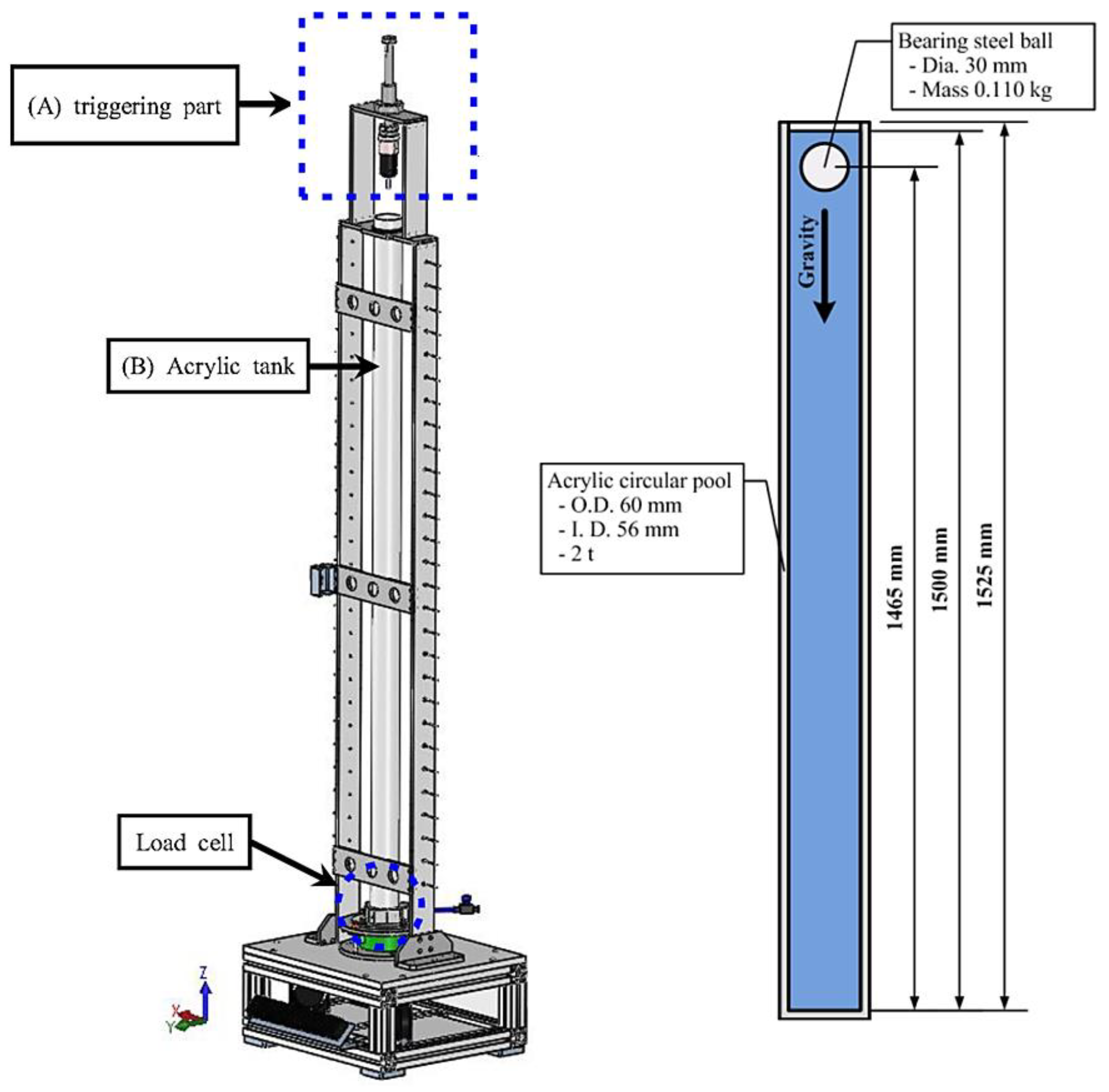
In order to review the feasibility of the numerical simulation method used in this study in advance, the FSI analysis method applied in this study was similarly simulated and compared with the study results of the underwater drop test of the bearing steel sphere [26]. Figure 4 shows the configuration and detailed dimensions of the testing device for the underwater drop test of the bearing steel sphere.

As shown in Figure 4, in the underwater drop test of the bearing steel sphere, with a diameter of 30 mm and mass of 0.11 kg, comprised the sphere being freely dropped into a tank with the water level of 1500 mm. Then, the change in position of the sphere was measured at the direction of gravity for the one second. In order to compare the accuracy of the FSI analysis based on the CEL method applied in this study with the existing test research results, a numerical simulation model was generated as shown in Figure 5. As shown in Figure 5, the 8-node solid Lagrangian element was used for the bearing steel sphere, and it was composed of 124 nodes and 24 elements. The Euler grid of fluid in the water tank used a hexahedron element and was composed of 77,959 nodes and 42,140 elements. The density and bulk modulus of elasticity for the fluid were applied as 1000 kg/m³ and 2.1 GPa, respectively. In order to reflect the interaction of the fluid–structure model, the surface of the bearing steel sphere, which is the common boundary domain where the two models are in contact, was set as the coupling surface. The grid size of the Eulerian model was applied densely by the rate of 25% compared to the element size of the Lagrangian model, the same as the soil penetration numerical simulation model in Section 2.3.

Figure 6 shows the representative results of the underwater drop movement distance of the sphere according to the fall time of the bearing steel sphere calculated from the FSI analysis.

As shown in Figure 6, the underwater drop movement distance of the bearing steel sphere varied with time variation due to the loss of kinetic energy caused to the interaction with the fluid. Figure 7 graphically represents the FSI simulation results of the underwater drop movement distance of the bearing steel sphere, comparing previous research results [26], the actual test, the computational fluid dynamics (CFD) analysis, and the theoretical solution.

As shown in Figure 7, both the FSI analysis results and the CFD analysis results, excluding the results of the theoretical solution, represented almost complete solution convergence and also had high agreement with the actual test results. Through a comparative review of the bearing steel sphere, it was verified that significant results can be derived from the FSI analysis based on the CEL method used in this study as applied to the underwater fall simulation. Such simulation is similar to the soil penetration simulation of anchor piles to determine the burial depth that can ensure the safety of subsea HVDC cables. The verified numerical modeling and simulation methods were applied to the simulation-based case studies for the anchor pile penetration to various types of soil in which the subsea HVDC cables are to be embedded.

The penetration characteristics resulting from the drop impact of the anchor pile were evaluated for each case where the seabed soil was a clay layer, sand layer, or clay–sand mixed layer, using the numerical model represented in Figure 3. Figure 8 shows the numerical simulation results of the anchor pile’s final penetration into each type of soil.

As shown in Figure 8, the maximum penetration depths of the anchor pile were calculated to be 3.85 m, 2.07 m, and 2.82 m, respectively, in the case of the clay layer, sand layer, and clay–sand mixed layer. The relative maximum penetration in the clay layer was found to be larger than that of the sand layer and the clay–sand mixed layer by 86% and 37% or more, respectively. The difference of penetration depth can be considered to be caused by the material properties of the soil. In particular, the internal friction angle is the angle between a horizontal plane and a straight line with respect to the normal and shear stresses acting on the soil particles, and is a soil property that represents the shear resistance characteristic. As represented in the material properties of soil in Table 1, the internal friction angle of the sand layer was much larger than that of the clay layer, and it can be seen that the relatively small penetration depth in the sand layer was affected by the internal friction angle.

The subsea HVDC cables in the southwest sea of Korea are generally installed at a burial depth of 3.0 m [2,4]. However, the numerical simulation results showed that, although subsea HVDC cables can be safely protected from the penetration of an anchor pile by the burial method itself alone in the sand layer and clay–sand mixed layer, an additional protective facility for subsea HVDC cables is required to be constructed in the case of the clay layer.

The variance of the anchor pile drop speed and the variance of the soil penetration in clay layer, sand layer, and clay–sand mixed layer are shown in Figure 9 and Figure 10, respectively.

The variance of drop speed and the variance of the soil penetration shown in Figure 9 and Figure 10, respectively, were measured in reference to the node at the extreme end of the anchor pile model. As shown in Figure 9, while the drop speed of the anchor pile rapidly decreased from the point in time when the soil penetration started in the case of the sand layer, the clay layer showed a characteristic where the drop speed decreased, after the maximum drop speed was constantly maintained, down to the soil penetration depth of about 2.0 m. In addition, the clay–sand mixed layer showed an intermediate type of drop speed behavior between the clay layer and the sand layer. As shown in Figure 10, the soil penetration of the anchor pile was maintained at the maximum penetration depth of 3.85 m at the point in time of 1.7 s after the drop of the anchor pile in the clay layer; it was maintained at the maximum penetration depth of 2.07 m at the point in time of 1.5 s after the drop of the anchor pile in the case of the sand layer; and it was maintained at the maximum penetration depth of 2.82 m at the point in time of 1.6 s after the drop of the anchor pile in the case of the clay–sand mixed layer. The convergence tolerance of the numerical simulation was considered as both displacement and energy convergence tolerances, and their values were set to 0.001, a default value recommended in the MSC.Nastran SOL700 module [15]. From the penetration depth variation of Figure 10, it was confirmed that the numerical solutions were converged.

Considering the decreasing drop speed characteristic of the anchor pile and the results of the maximum soil penetration time, the soil burial safety of the sand layer was superior to that of the clay layer and the clay–sand mixed layer.

3. Verification Test for Soil Penetration of Anchor Pile

3.1. Field Verification Test

To verify the validity of the numerical simulation results for the soil penetration of the anchor pile, a field verification test was conducted using the anchor pile produced to have the same specifications as that of the numerical analysis model and using soil whose properties are the same as the material properties of the soil applied to the numerical simulation. The field verification test was conducted in the verification test site of KEPCO, located in Gochang, Jeollabuk-do, Korea. The verification test site was built on a site of 730,000 m²; facilities that can perform comprehensive verification tests for 31 electric power technology fields were included in the test site. In order to conduct the field verification test for the soil penetration of the anchor pile, a trench with a depth of 5 m, a width of 3 m, and a length of 5 m was generated, and three types of seabed soil were filled into the trench. The anchor pile was also mounted on a 20 ton grade mobile truck crane and dropped into the trench from a height of 7.18 m. The configuration of the field verification test for the soil penetration of the anchor pile is shown in Figure 11.

As shown in Figure 11, the drop condition of the anchor pile for soil penetration was materialized by connecting a cable mounted on the crane that could secure a drop height of 18.5 m or more to the top of an anchor pile. In addition, the test conditions for the soil penetration of the anchor pile were organized by securing spaces of 3.0 m depth in the ground of the general soil test site and then filling them with clay, sand, and clay–sand mixed layers. In the field verification test, the drop height of the anchor pile was set to 7.18 m from the ground, the same as that of the numerical simulation model shown in Figure 3, and the drop speed at the time of soil penetration was measured to be 12.4 m/s. The maximum soil penetration was measured at a point in time of 60 s or more after the anchor pile was dropped, to minimize the variability of penetration. In addition, the maximum soil penetrations resulting from the drop of the anchor pile for three times on the clay, sand, and clay–sand mixed layers were measured, and the average values were calculated, taking into account the possibility for errors to occur depending on the drop test conditions. Figure 12 shows the test result for the state of maximum soil penetration of the anchor pile into each soil type.

As for the method of measuring the maximum soil penetration, the penetration depths were measured by dropping the anchor pile painted with different colors at a constant interval of height for the field verification test, as shown in Figure 11 and Figure 12. Then, markers were attached on the surface of the anchor pile when the penetration was completed. The soil penetration verification test results of the anchor pile were put in order and are shown in

Table 2. Field verification test results for soil penetration of anchor pile.

Soil Type	Max. Penetration Depth
	Test #1	Test #2	Test #3	Average	Coefficient of Variance
Clay	3.86 m	3.91 m	4.07 m	3.95 m	2.78%
Sand	1.86 m	1.93 m	1.85 m	1.88 m	2.32%
Clay–sand	2.66 m	2.77 m	2.83 m	2.75 m	3.14%

.

As shown in Table 2, the maximum penetration depths were in the range of 3.86 m to 4.07 m, and the average value was 3.95 m in the case of the clay layer. The maximum penetration depths of the sand layer were in the range of 1.86 m to 1.93 m, and the average value was 1.88 m. The maximum penetration depths of the clay–sand mixed layer were in the range of 2.46 m to 3.03 m, and the average value was 2.75 m. The mean absolute deviations of the test results in the clay layer, sand layer, and the clay–sand mixed layer were calculated to be 8.2%, 3.3%, and 6.2%, respectively, and the consistency of the test result was judged to have been secure, considering that it was a field verification test for the soil penetration resulting from the drop of an anchor pile. The coefficient of variance for the three test results was computed to be 2.28%, 2.32%, and 3.14%, and an international test standard regarding the soil penetration required that the coefficient of variance of the test results for the same soil was less than about 10% [27]. Therefore it can be seen that the number of tests and the test procedures were reliable.

3.2. Comparison of Simulation and Test Results

To quantitatively review the validity of the maximum soil penetration result by soil type calculated from the numerical simulation for the soil penetration of the anchor pile, the simulation results were summarized and compared with the average values of the field verification test results, as presented in

Table 3. Comparison of anchor pile penetration results.

Soil Type	Max. Penetration Depth (m)		Error
	Simulation	Test (Average Results)
Clay	3.85	3.95	2.5%
Sand	2.07	1.88	10.1%
Clay–sand	2.82	2.75	2.6%

.

As shown in Table 3, the error rates of the numerical simulation results as compared with the average values of the verification results were 2.5%, 10.1%, and 2.6% in the clay layer, the sand layer, and the clay–sand mixed layer, respectively. When considering that it is the numerical simulation for the fluid–structure interaction phenomenon of the soil penetration resulting from the drop impact of an anchor pile, the error rates from the field verification test results shown in Table 3 were judged to be at reasonable levels. The FSI analysis method for the soil penetration resulting from the drop of the anchor pile carried out in the present study can be usefully utilized for the determination of the burial depth that can minimize the risk of damage to subsea HVDC cables using burial-type protection methods. In addition, it is thought that the numerical simulation method based on FSI analysis can be efficiently applied also to the analysis of the soil penetration characteristics of the subsea HVDC cable hazards in the form similar to the anchor pile.

4. Conclusions

In this study, the soil penetration characteristics of anchor piles, depending on the soil type, were evaluated using FSI analysis and field verification tests to determine the burial depth that can ensure the safety of subsea HVDC cables embedded in the southwest coast of Korea during the soil penetration of anchor piles for aquaculture works, which are one of the major reasons for subsea HVDC cable breakage. Numerical simulations were carried out using the FSI analysis method to evaluate the soil penetration characteristics of anchor piles, and the numerical simulation results were verified through the comparison of the field verification test results.

The numerical simulation results showed that the relative final penetration depth into the clay layer was larger than that into the sand layer and the clay–sand mixed layer, by 86% and 37% or more, respectively. Such results showed that considering the ordinary 3.0 m burial depth of the subsea HVDC cables installed in the southwest sea of Korea, an additional protective facility for subsea HVDC cables is required to be constructed in the case of clay layers. Meanwhile, subsea HVDC cables can be safely protected from the penetration of anchor piles by the burial method alone in sand layers and clay–sand mixed layers. In the field verification test, the numerical simulation results were compared with the average values obtained by measuring the maximum soil penetration depths of the anchor pile. The error rates of the numerical simulation results compared with the verification test results were 2.5%, 10.1%, and 2.6% in the clay layer, the sand layer, and the clay–sand mixed layer, respectively. Considering that it is a numerical simulation for the fluid–structure interaction phenomenon of the soil penetration resulting from the drop impact of an anchor pile, the error rates from the field verification test results were judged to be at reasonable levels. The FSI analysis method of the soil penetration resulting from the drop of the anchor pile presented in the present study can be utilized for the determination of the burial depth that can minimize the risk of damage to burial-type subsea HVDC cables in the southwest coast of Korea, and it is thought that the method can be efficiently applied also to the analysis of the soil penetration characteristics of various forms of hazards to subsea HVDC cables. Since the safety guarantee of subsea HVDC cable facilitates the operation of social infrastructure, the practical use of the results of this study has public engineering significance. The results of this study also can be extended and utilized for FSI analysis–based performance verification to secure design safety in various civil and marine engineering fields.

In future research, the authors plan to expand the present study results to conduct studies on soil penetration resulting from the drop impact of ship anchors and soil concentrations, and on the breakage phenomenon of various forms of subsea HVDC cable protection structures based on three-dimensional FSI analysis.