An Improved Version of ETS-Regression Models in Calculating the Fixed Offshore Platform Responses

Abstract

An offshore structural design should accurately calculate wave loads and structural responses acting on slender cylinders. The hydrodynamic drag-dominated force was always challenging, hence the hydrodynamic wave loading became a complex solution; it led to a nonlinear relation between the wave force and responses caused by the diffracted and radiated waves, which was included in Morison’s equation. For more consistency in the structural assessment, the linearised drag–inertia force was considered in model development, such as an improved version of the efficient time simulation regression (ETS-Reg) procedure that was introduced. The study aimed to improve the prediction of structural responses using the predetermined linear, polynomial, and cubic regression models. These simulations were performed focusing on high sea state conditions without wave-induced current effects. In order to evaluate the level of accuracy, the recent ETS-Reg models were compared and validated using the Monte Carlo time simulation (MCTS) method. An amended ETS-Reg model, known as the ETS-Reg_LR model, was also compared with the previous results obtained using the conventional ETS-Reg models (ETS-Reg_SE), leading to better structural response calculations.

1. Introduction

Based on the presumptions of potential flow nearby small structure bodies, Morison’s equation (ME) was adequate to represent the hydrodynamic behavior (Mukhlas et al., 2016). The ME represented the total load as a sum of two contributions: nonlinear drag and linear inertia forces. It formed a way to express the equation in order to determine additional damping (drag force) and added mass (inertia force) [1]. However, difficulties in hydrodynamic response analysis were continuously complicated phenomena that were often considered non-Gaussian characteristics [2]. Therefore, the nonlinear drag term was always an issue that influenced the consistency of offshore structural response estimation.

The linearisation of the nonlinear force expression was a common technique for resolving this inconsistency. This approach was initially introduced by [3,4], and continued by other researchers for calculation improvement in their studies [5,6,7,8]. As stated by [9], a relative study of the linear and nonlinear forms of the wave-induced force from Morison’s equation was conferred and derived. In different techniques, the nonlinear drag term in Morison’s equation was also linearised by least square methods [10].

Following the prior findings, the recent practice also implemented a similar approach by linearising the wave force component in Morison’s equation as a modified model of development. This paper is an extended version of the previous paper by [11,12], who offered a striking finding in the development of the empirical regression model. In fact, a simplified approach was found through the efficient time simulation regression (ETS-Reg) procedure in order to assess the complex hydrodynamical wave load-induced responses. As reviewed in that paper, the structural response of the structure was calculated based on applying the ETS-Reg_SE model.

However, the earlier ETS-Reg procedure was developed based on surface elevation as the primary input parameter for model development, which is why the structural response estimation was always an under-predicted phenomenon. For that reason, a proposed probabilistic model was utilised to simulate the more accurate structural responses by applying an improved version of the ETS-Reg procedure to obtain reliable results. The amended ETS-Reg_SE model, known as the ETS-Reg_LR model, was presented by introducing linearised responses as the revised input parameter in model development. As the same practice was implemented in [12,13], this recent paper consisted of three regression models: linear, polynomial, and cubic were improved in predicting the structural responses.

A parametric analysis was conducted to clarify the distinction between the wave loads-induced responses determined by the ETS-Reg_SE and ETS-Reg_LR models. These ETS-Reg models were measured in 100-year extreme response models, which consider low and high-sea sea state conditions with no current impacts. Both ETS-Reg models were compared and validated using the benchmark Monte Carlo time simulation (MCTS) method to examine the level of accuracy.

2. Platform Specifications and Wave Modelling Analysis

This section may be divided into two subheadings. Firstly, it consists of the test structure model accompanied by specific descriptions, which is similar to a fixed jack-up platform. Secondly, the evaluation of the offshore structural responses is calculated numerically regarding ocean wave hydromechanics. Lastly, the MCTS procedure is used as a reference to predict the extreme values of the short-term probability distribution.

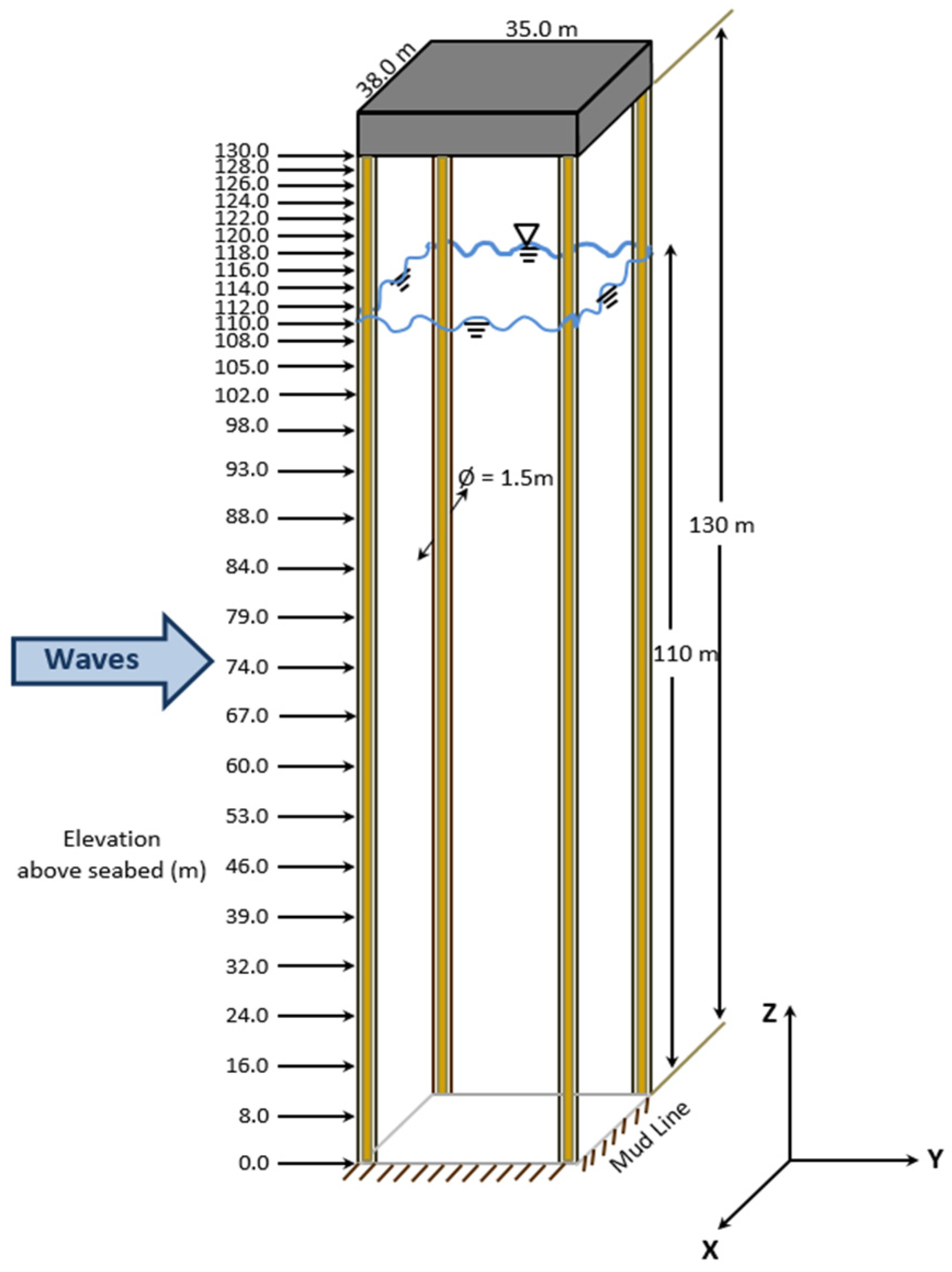
2.1. Test Structure Specifications and Offshore Platform Models

The calculation of structural responses was based on the given features of offshore platforms. An ocean structure is subjected to the buildup of organic marine growths. The fluid flow behaviours around naturally roughened circular cylinders with a drag coefficient (Cd) and inertia coefficient (Cm) are equal to 1.05 and 1.20, respectively. Hydrodynamic coefficients are influenced by marine growths and natural roughness. Specifications of the jacket structural model admitted in this study were at an ocean depth of 110 m in the North Sea. These legs had a diameter of 1.5 m and a thickness of 0.04 m [14].

Figure 1 presents a fixed platform comprised of a four-legged platform that is a large-diameter tubular leg frame pile fixed to the seabed. The scattered load on each leg was designated by 30-point loads that reached a total number of nodal loads [15,16]. The total mass was 17,665 tonnes, and the square cross-section jacket measured 38 m × 35 m (plan view) on the platform deck.

Waves from the environment mostly caused the structural loads. The actual data were used to assess two configurations: offshore platforms and environmental met-ocean. Atkins Ltd. (Epsom, UK) provided the structural data and the Health and Safety Executive (Bootle, UK) granted environmental data for Forties Field in the North Sea region. Based on ocean wave hydromechanics, the fast Fourier transform (FFT) mathematical tools were used to simulate the wave hydrodynamics of sea surface elevation, wave loadings on slender structures, and their corresponding structural responses.

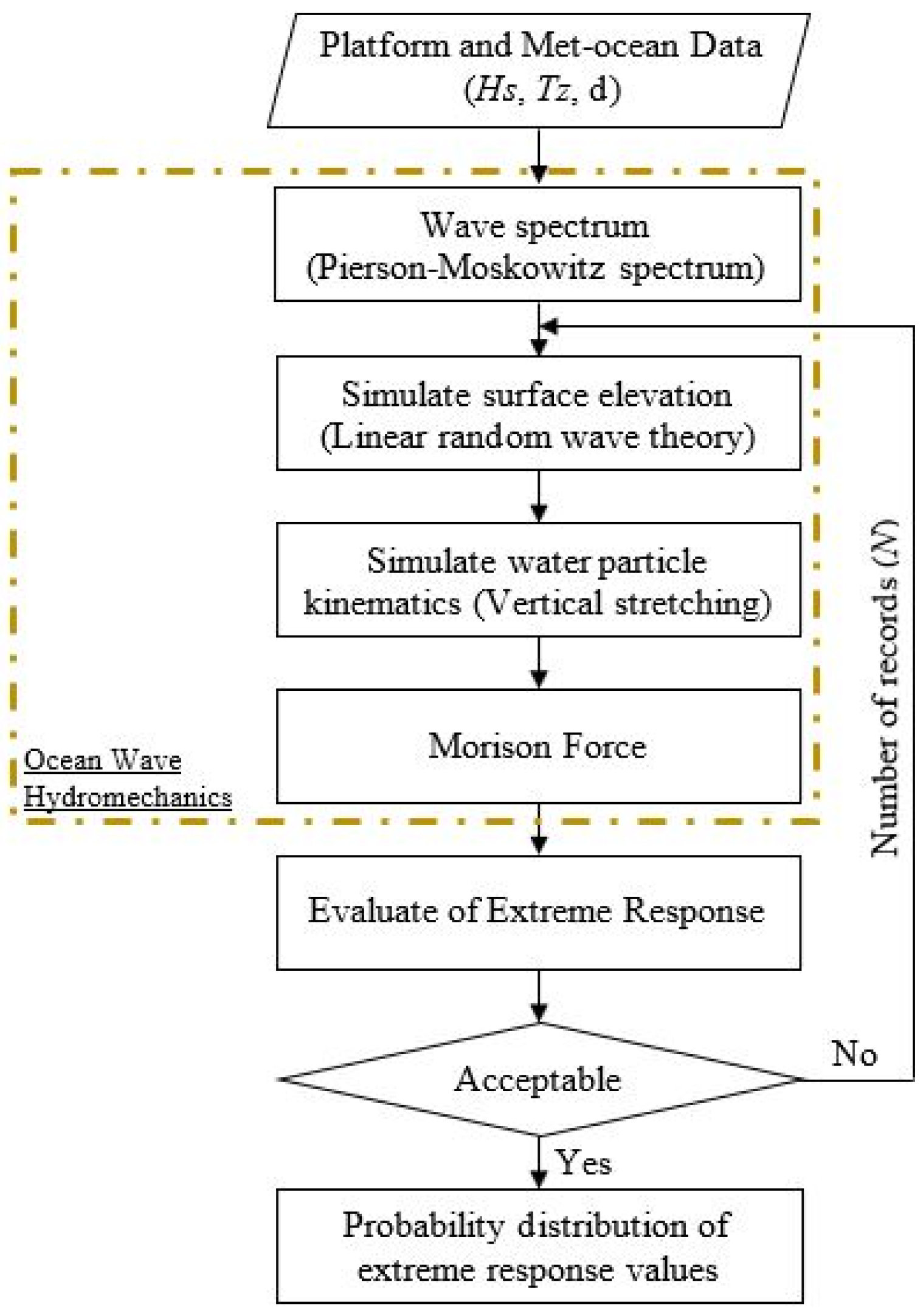
2.2. Numerical Simulation of Offshore Structural Responses

Simulations were used to bring a numerical model of a calculation scheme into the real world using computer capabilities. Currently, in the presence of advanced software availability [17,18], stochastic analysis is feasible to carry out a robust time-domain analysis where the complicated wave loads were integrated into a numerical ocean model [19]. In the wave scheme shown below, artificial ocean waves could be simulated as associated with several ocean wave models [20].

Generic Spectrum: According to wave [21], the generic spectrum model could be used to generate waves. The wave spectrum, such as the P-M spectrum, was used in this current study, as described by Equation (1):

$$S_{\eta }{\left(f\right)}_{PM}=\frac{H_s^2}{4\pi T_z^4{f}^5}exp\left(\frac{1}{\pi T_z^4{f}^4}\right)$$

(1)

where S_η is the surface elevation frequency spectrum, H_s is the significant wave height (m), T_z is the mean zero up-crossing period (s), f is wave frequency (Hz), and π is a mathematical constant of 3.142.

Linear Random Wave Theory: Transforming the wave spectrum S_η(f) to wave elevation η(t) could be performed by an inverse FFT (IFFT) method. According to linear random wave theory (LRWT), an irregular sea could be described as a superposition of many different regular waves [22], as represented by Equation (2):

$$\eta \left(t\right)={\displaystyle \sum }_{i=1}^{NW=N/2}{A}_{i}cos\left(2\pi f_{i}t-k_{i}x-{\phi }_i\right)$$

(2)

where η is the water surface elevation, NW is the total wave number used, x is the distance from wave origin, t is time, f_i is set of wave frequency, k is wave number, φ_i random phase angle (0 to 2π), and A_i wave amplitudes.

Water Particle Kinematics: LRWT was the method used for simulating the visualisation of water particle kinematics in various nodes of offshore structures [23,24,25]. The water particle equations were defined by using Equations (3) and (4):

$$u\left(x,t\right)=A_{i}2\pi f_i\frac{\mathit{cosh}\left(k_i\left(z+d\right)\right)}{\mathit{sinh}\left(k_{i}d\right)}cos\left(k_{i}x-{\omega }_{i}t\right)$$

(3)

$$\dot{u}\left(x,t\right)=A_i{\left(2\pi f_i\right)}^2\frac{\mathit{cosh}\left(k_i\left(z+d\right)\right)}{\mathit{sinh}\left(k_{i}d\right)}sin\left(k_{i}x-{\omega }_{i}t\right)$$

(4)

where u is the water particle velocity, u′ is the water particle acceleration, x is the horizontal direction, z is the elevation above the seabed, t is time, d is water depth, k_i is wave number, ω_i is angular frequency, 2πf (rad/s), and A_i wave amplitudes.

Morison’s Equation: For this fixed offshore platform, Morison-based analysis was more suitable, since the wave-induced horizontal force per unit length was on a vertical submerged cylinder [26]. Morison’s equation (ME) was the sum of a nonlinear drag and a linear inertial form, stated by Equation (5):

$$F_{wave}\left(z,t\right)=\frac{1}{2}\rho C_{D}D\stackrel{r_{drag}}{\overbrace{\left(u-\dot{x}\right)\left|u-\dot{x}\right|}}+\frac{\pi }{4}\rho C_M{D}^2\stackrel{r_{inertia}}{\overbrace{\dot{u}}}$$

(5)

where F_wave is wave load, F_drag is drag force, F_inertia is inertia force, C_d is drag coefficient, C_m is inertia coefficient, ρ is water density, D is cross-sectional area of the cylinder section, and x′ is the structure velocity.

Linearisation of Morison’s Equation: This method was known as a modification of Morison’s equation. The linearisation was to simplify the calculation based on the absolute velocity and acceleration technique, which minimises the error between the original nonlinear and linear form [27]:

$$r_{L,drag}={\alpha }_1{u}_1+{\alpha }_2{u}_2+{\alpha }_3{u}_3+\cdots {\alpha }_n{u}_n$$

(6)

$$r_{L,inertia}={\beta }_1{\dot{u}}_1+{\beta }_2{\dot{u}}_2+{\beta }_3{\dot{u}}_3+\cdots {\beta }_n{\dot{u}}_n$$

(7)

For simplification, the common approach was to utilise the least square error (LSE) method in order to determine factors for the equivalent linear form. By minimising E[e²] and E[e′²], the α and β coefficients were determined as follows:

$$e=r_{drag}-r_{L,drag}=r_{drag}-{\alpha }_1{u}_1+{\alpha }_2{u}_2+{\alpha }_3{u}_3+\cdots {\alpha }_n{u}_n$$

(8)

$$e’=r_{inertia}-r_{L,inertia}=r_{inertia}-{\beta }_1{\dot{u}}_1+{\beta }_2{\dot{u}}_2+{\beta }_3{\dot{u}}_3+\cdots {\beta }_n{\dot{u}}_n$$

(9)

where r_L,_drag and r_L,inertia are linearised drag and inertia force.

Structural Responses: With reference to those mentioned above, the wave load of quasi-static response for base shear (BS) and overturning moment (OTM), respectively, could be calculated as follows:

$$\mathrm{BS}={\displaystyle \sum }_{i=1}^{NS}\left(F_i\times ∆l_i\right)$$

(10)

$$\mathrm{OTM}={\displaystyle \sum }_{i=1}^{NS}\left(F_i\times ∆l_i\times z_i\right)$$

(11)

where NS is number of nodal loads, $F_i$ is Morison load per unit length at node i, $∆l_i$ is length of the element associated with node i, and $z_i$ is the elevation of node i from the seabed, as illustrated in Figure 1.

2.3. Evaluation of Short-Term Probability Distribution of Extreme Offshore Structural Responses Using MCTS Method

A simple approach used to find the extreme value of short-term probability distribution was the MCTS method [28,29]. This procedure could be analysed based on ocean wave hydromechanics (numerical modelling) in the preceding section in order to predict a response record (beginning with a simulated surface elevation record), as shown in Figure 2. Next, the technique was repeated as many times as necessary to acquire a large number of extreme response records. The simulated extreme values were then ranked from smallest to largest.

Following Equation (12), the plotting position equation for the Gumbel distribution [30] was adopted to determine the probability distribution value for each ranking extreme value. The short-term probability distribution of responses was computed in this study using a record of 10,000 responses with a length of 128 s.

$$P(i\le x_i)=p_i=\left(\frac{i-0.44}{n+0.12}\right), i=1,2,3,4\dots n$$

(12)

where i is the rank of the order statistic associated with $p_i$ of the data point, n is the total number of points.

3. Development of Improved ETS-Regression Procedures

According to [11,12], an ETS-Regression (ETS-Reg) model was developed relying on two main variables between their input variables (extreme surface elevation) and its corresponding output variables (extreme responses), so-called the ETS-Reg_SE model. Based on this excellent duo-relationship, there was a possibility to build regression models from the relationship between input–output parameters. This straightforward model could be used to predict time-consuming 100-year structural responses. However, the ETS-Reg model is restricted to particular sea state conditions, with the level of accuracy decreasing as the significant wave height, H_s = 5 m.

In this current paper, the improvement of ETS-Reg models would be extended using the revised input variable of linearised responses, known as the ETS-Reg_LR model. Following the same approach of previous ETS-Reg procedures, the recent model development was also introduced to several regression models (linear, polynomial, and cubic). In this study, the least-squares Pearson’s correlation–regression approach was preferred for the development of the regression models alongside the hindcast data obtained [31], as illustrated in Figure 3. According to the least square error (LSE) procedure, the line (linear regression model) and curve-fitting (nonlinear regression model) techniques would be used to derive simple functions. Therefore, the unknown model coefficients for each model were solved by Cramer’s rule [32].

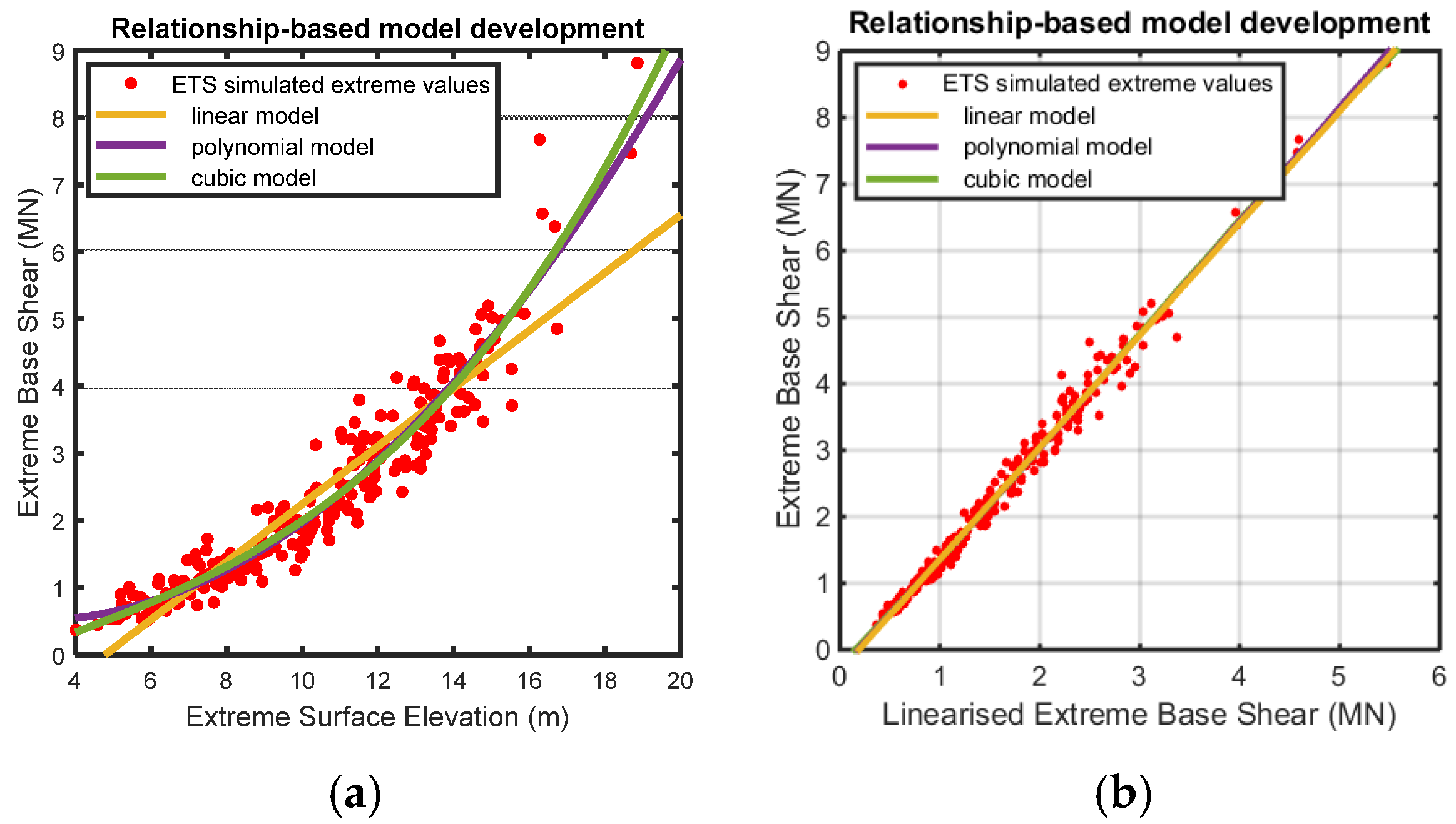
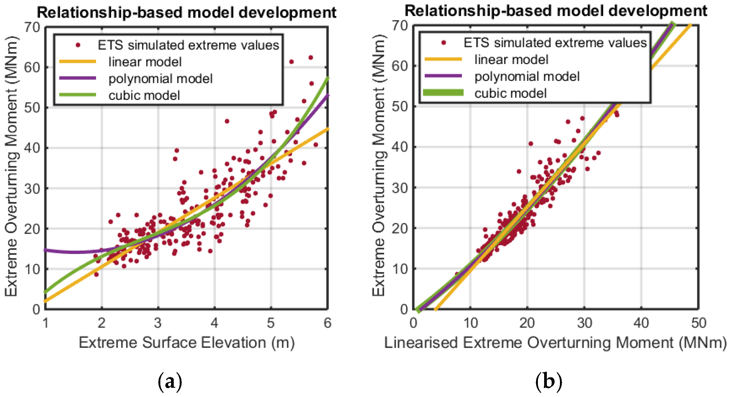
3.1. Relationships of ETS-R_SE and ETS-R_LR

The pioneer ETS method was presented by [15] and offered the advantage of a relationship between extreme values of surface elevation and responses. Therefore, an extended ETS method, known as the ETS-Reg model, was introduced. Regarding Pearson’s correlation analysis,

Table 1. The coefficient of correlation between two categories of ETS relationships (scatterplot) for the conditions of low and high sea states (H_s) without current (U = 0.0 m/s) impacts regarding the total quasi-static base shear and overturning moment responses.

	Base Shear		Overturning Moment
Type of ETS-Reg (correlation-r)	ETS-RSE	ETS-RLR	ETS-RSE	ETS-RLR
	r	r	r	r
Significant wave height, Hs = 15 m (high sea state)
	0.9408	0.9931	0.9376	0.9922
Significant wave height, Hs = 5 m (low sea state)
	0.8444	0.9626	0.8360	0.9528

shows the intensity of the relationship via correlation-r values for both the ETS (ETS-R) relationships with different input parameters at low and high-sea sea state conditions. The ETS-Relationship-based surface elevation (SE) input is the term given to this type of ETS-R_SE, in the meanwhile, the ETS-Relationship-based linearised response (LR) as the revised input was named ETS-R_LR. In this preliminary analysis, the wave conditions of H_s = 5 and 15 m without the effect of currents were selected in order to examine the establishment of relationships.

According to the findings in Table 1, the strength of the relationship became less proportional to decreasing sea state conditions. Secondly, the relationship based on linearised responses (ETS-R_LR) as the input parameters observed higher correlation-r values instead of surface elevation (ETS-R_SE). The cubic-based regression model had the highest correlation-r-value among the regression model types when compared to the two other types, linear and polynomial.

3.2. Regression Models of ETS-Reg_SE and ETS-Reg_LR

Figure 4a demonstrates the relationship between extreme surface elevations proportional to the extreme base shear responses for high sea state conditions without the impact of currents. As a result, in terms of total quasi-static base shear responses, an effective coefficient of correlation (r = 0.9408) was acquired where this ETS-R_SE relationship was considered for the development of the ETS-Reg_SE model. Figure 4b shows that the improvement of the relationship scatterplot offered a strong correlation coefficient (r = 0.9931) rather than the ETS-R_SE relationship. The improved relationship was based on the updated input parameter of linearised responses, which is the output of the linearised ME (refer Figure 3). Thus, the ETS-Reg_LR model development was based on the ETS-R_LR relationship. The amended version of the ETS-Reg_SE model, known as the ETS-Reg_LR model, made a significant improvement in both relationship and model development.

For low sea state conditions without the effect of currents, Figure 5a shows the coefficient of correlation (r = 0. 8360) was obtained in terms of total quasi-static overturning moment responses, and this ETS-R_SE relationship was considered for the formation of the ETS-Reg_SE model. Figure 5b demonstrates that the improved ETS-R_SE relationship scatterplot increased the coefficient of correlation up to r = 0. 9528. Thus, this enhanced correlation was also derived from the linearised responses as the input parameter, which improved model development.

Table 2. Types of ETS-Reg models regarding the coefficient of determination for the low and high sea state (H_s) conditions without current (U = 0.0 m/s) impacts regarding total quasi-static base shear and overturning moment responses.

	Base Shear		Overturning Moment
ETS-Reg Models	ETS-RegSE	ETS-RegLR	ETS-RegSE	ETS-RegLR
	r2	r2	r2	r2
Significant wave height, Hs = 15 m (high sea state)
Linear	0.8851	0.9862	0.8792	0.9844
Polynomial	0.9284	0.9863	0.9304	0.9845
Cubic	0.9296	0.9864	0.9317	0.9846
Significant wave height, Hs = 5 m (low sea state)
Linear	0.7131	0.9265	0.6988	0.9078
Polynomial	0.7360	0.9291	0.7345	0.9103
Cubic	0.7377	0.9292	0.7386	0.9105

demonstrates the coefficient of determination (r²) involving the linear, polynomial, and cubic regression models. According to the relationship pattern in Figure 3, the relationship between ETS-Reg_LR was far more significant than the relationship between ETS-Reg_SE, which indirectly improved all ETS-Reg models. Overall, the ETS-Reg_LR models were satisfactory, rather than the ETS-Reg_SE models, particularly when applying the linearised responses as the input variable in the relationship instead of surface elevation.

Similar to the relationship findings (correlation-r values), the ETS-Reg_LR based on the cubic model was better than the ETS-Reg_SE cubic model. The r-squared of the ETS-Reg_LR cubic model was 0.9864, which was much higher than the ETS-Reg_SE cubic model, equal to 0.9296. Due to this evidence, the ETS-Reg_LR cubic model was expected to influence the accuracy level of the probability distribution of a 100-year extreme response prediction.

4. Derivation of Short-Term Probability Distribution of Extreme Offshore Structural Responses

The short-term probability distribution of ETS-Reg models would be compared to the benchmark of MCTS probability distribution for the 100-year extreme responses.

4.1. Preliminary Analysis of Extreme Responses by Three Types of ETS-Reg Models

In order to provide a good result, the level of accuracy regarding three types of ETS-Reg model development was required to be examined with the benchmark of MCTS procedures. This prediction would be plotted on the 100-year short-term probability distribution of extreme responses.

Table 3. ETS-Regression of different empirical models in calculating the P₁₀₀-year short-term responses for total base shear quasi-static responses and without current. H_s = 15 m (P₁₀₀MCTS = 11.1459 mega Newton (MN)).

Method	Prediction		Responses Ratio
	ETS-RegSE	ETS-RegLR	ETS-RegSE MCTS	ETS-RegLR MCTS
Linear	12.0808	11.4266	1.0839	1.0252
Polynomial	10.4922	11.3804	0.9413	1.0210
Cubic	10.0723	11.3220	0.9037	1.0158

demonstrates the ETS-Reg procedures with linear, polynomial, and cubic-based regression models used in calculating the predicted 100-year responses (P100) for high sea states without current impact.

As observed in Table 3, the prediction of 100-year extreme responses between the ETS-Reg_SE and the ETS-Reg_LR model was examined with the MCTS method. The benchmark of the MCTS method predicted was 11.1459 (≈11.15) MN. As shown in Figure 6, the comparison of ETS-Reg_LR models among linear, polynomial, and cubic types was validated for the probability distribution of 100-year extreme responses. Since the strength of relationships and model development via correlation-r alongside r-squared values were related, it affects the accurate prediction of 100-year responses obtained. It could be observed that the regression-based cubic model was only preferred for validation purposes compared to linear and polynomial models.

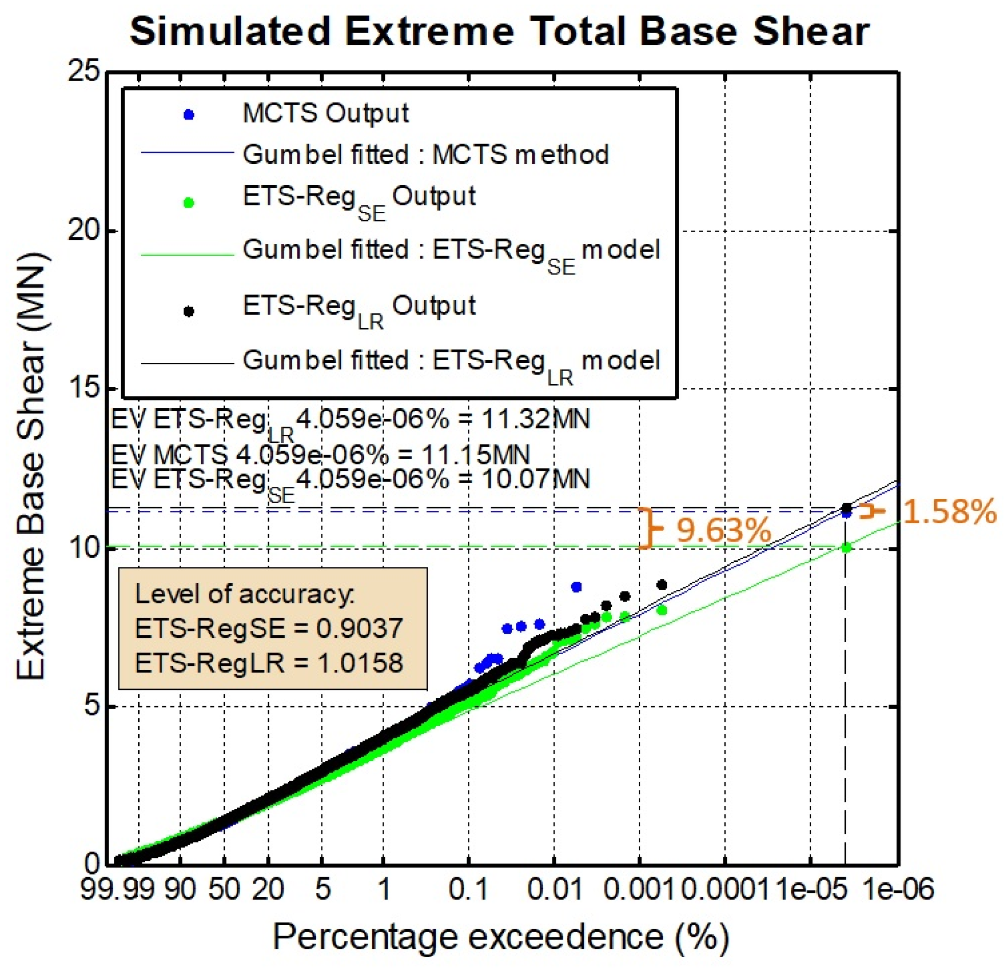
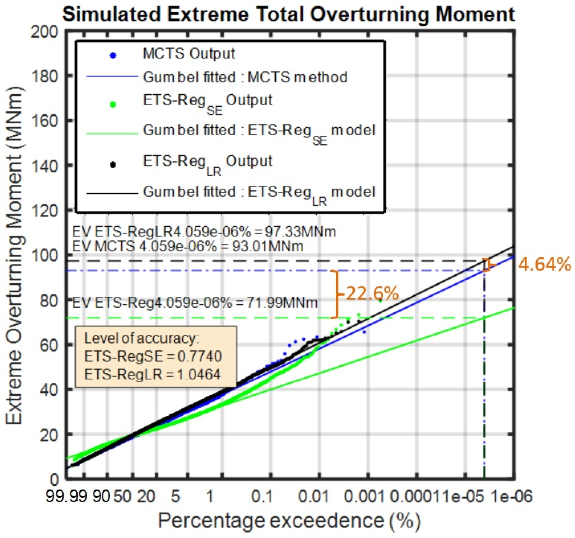
4.2. Level of Accuracy of Extreme Responses by ETS-Reg Models

Syed Ahmad et al. [13] studied that the accuracy level based on ETS-Reg_SE models corresponded procisely to the relationship results, as presented in Part 1 in [12]. Similar to the previous study, the 100-year response reduced significantly as the high H_s decreased to the low H_s in terms of measured accuracy ranges. In the current findings,

Table 4. Comparison of the MCTS method with the ETS-Reg_SE and ETS-Reg_LR models for 100-year responses with the low and high sea state (H_s) conditions without current (U = 0.0 m/s) impacts.

Responses	Base Shear			Overturning Moment
Methods	Ratio			Ratio
	MCTS (MN)	ETS-RegSE MCTS	ETS-RegLR MCTS	MCTS (MNm)	ETS-RegSE MCTS	ETS-RegLR MCTS
Significant wave height, Hs = 15 m (high sea state)
Total responses	11.1459	0.9037	1.0158	983.7499	0.9316	1.0087
Significant wave height, Hs = 5 m (low sea state)
Total re-sponses	0.9795	0.8037	1.0453	93.0112	0.7740	1.0464

shows the MCTC methods’ deviation ratio of 100-year extreme responses had comparable diversity to ETS-Reg_SE and ETS-Reg_LR models. The result shows that an improvement was made by the ETS-Reg_LR model, with an accuracy range of 96–99 percent. In contrast, the accuracy level of the ETS-Reg_SE models was made approximately 77–93 percent. Thus, the increment results show an improved approach with the ETS-Reg_LR model for more accurate structural response calculation.

As pre-analysis studied in Section 4.1, the ETS-Reg models were developed based on cubic regression models. Figure 7 displays the predictions by ETS-Reg_SE and ETS-Reg_LR cubic-based models were 10.0723 and 11.3220 MN, respectively. The analysis was considered for the high sea state regarding the total quasi-static base shear responses. Based on these different outcomes, the ETS-Reg_LR proved that the ratio response was 1.0158 compared to the ETS-Reg_SE equal to 0.9037. That meant the ETS-Reg_LR model provided the highest level of accuracy with a minimal error value of around 1.58% in predicting the 100-year extreme responses as validated by the MCTS method. As expected, the improved relationship significantly impacted the model accuracy of ETS-Reg_LR, which was the most accurate result.

The result was an underestimated value for the low waves, with a significant percentage error when the validation between the MCTS method and ETS-Reg_SE models was examined. With the presence of the ETS-Reg_LR model to improve this particular sea state, the error was reduced from 22.6 to 4.64 percent. Figure 8 demonstrates that the predictions by ETS-Reg_SE and ETS-Reg_LR models were 71.9907 and 97.3269 MNm, respectively. Therefore, the improvement of the relationship associated with the regression model development significantly influenced predicting the 100-year extreme responses, which contributed to a better level of accuracy.

5. Conclusions

This study has concluded the improved version of ETS-Regression model development output based on the short-term 100-year of extreme offshore structural responses, and the results are summarised as follows:

• In the current study, the comparison of the probability distribution of quasi-static extreme responses values was validated between the MCTS and ETS-Regression method. This study was considered for a single sea state without the current impact. Moreover, the structures exposed to the load intermittency in the splash zone were included.
• The simplified development of the ETS-Reg model offered another approach to boost numerical calculation based on the probabilistic time domain. Applying this method could reduce computational demand as required by the MCTS method. Due to its accuracy, the ETS-Reg models proved equivalent to the MCTS method used in the probability distribution of extreme responses.
• This ETS-Regression method provided: (i) no need for extensive simulations, and (ii) no requirement to pass through several procedures of calculations in order to estimate 100-year extreme responses.
• The ETS-Reg_SE model was based on the input of surface elevation, whereas the ETS-Reg_LR model was based on the input of linearised responses as the revised input parameter of ETS-Relationship. Thus, the prediction of 100-year responses by ETS-Reg_LR had better accuracy when compared to ETS-Reg_SE for high sea state conditions without a current impact.
• As revealed in Table 4, this result shows that accurate structural response values could be achieved using the linearised response as the new input variable of relationships in developing the regression models.
• The ETS-Reg_LR model was good at predicting the 100-year-old extreme responses with a 96% to 99% level of accuracy level in comparison to its benchmark of the MCTS procedure. In contrast, the ETS ETS-Reg_SE model produced a lower level of accuracy of 77% to 93%.
• Further research is necessary to consider the wave current since it substantially impacts the drag component of the Morison force.
• The simulation used in this work was also restricted to a single sea state. It is well recognised that the sea surface is not stationary in actual conditions and that a wide range of sea states can be used to characterise it. Therefore, using the long-term distribution to determine the 100-year responses to design the structure is advised.
• The most significant loading source for offshore structural design is typically the load caused by wind-generated random waves. A nonlinear wave analysis, such as Stokes wave theory, solitary wave theory, cnoidal wave theory, stream function, or standing wave theory, is recommended to approximate a realistic ocean wave for an accurate prediction of the severe offshore structure response.

References

1. Hansen, H.F.; Kofoed-Hansen, H. An Engineering-Model for Extreme Wave-Induced Loads on Monopile Foundations. In Proceedings of the 36th International Conference on Ocean, Offshore and Arctic Engineering, Trondheim, Norway, 25–30 June 2017; p. V03BT02A014. [Google Scholar]
2. Machado, U.E. B Statistical Analysis of Non-Gaussian Environmental Loads and Responses. Ph.D. Thesis, Lund University, Lund, Sweden, 2002. [Google Scholar]
3. Borgman, L.E. Random Hydrodynamic Forces on Objects. Ann. Math. Stat. 1967, 38, 37–51. [Google Scholar] [CrossRef]
4. Borgman, L.E. Spectral Analysis of Ocean Wave Forces on Piling (Coastal Engineering Conference in Santa Barbara, California, October 1965). J. Waterw. Harb. Div. 1967, 93, 129–156. [Google Scholar] [CrossRef]
5. Terro, M.J.; Abdel-Rohman, M. Wave Induced Forces in Offshore Structures Using Linear and Nonlinear Forms of Morison’s Equation. J. Vib. Control. 2007, 13, 139–157. [Google Scholar] [CrossRef]
6. Siow, C.; Koto, J.; Abyn, H.; Khairuddin, N. Linearized Morison Drag for Improvement Semi-Submersible Heave Response Prediction by Diffraction Potential. J. Ocean Mech. Aerosp. Sci. Eng. 2014, 6, 8–16. [Google Scholar]
7. Housseine, C.O.; Monroy, C.; Bigot, F.; Neuilly-sur-Seine, F. A New Linearization Method for Vectorial Morison Equation. In Proceedings of the 30th International Workshop on Water Waves and Floating Bodies, Bristol, UK, 12–15 April 2015; pp. 12–15. [Google Scholar]
8. Housseine, C.O.; Monroy, C.; de Hauteclocque, G. Stochastic Linearization of the Morison Equation Applied to an Offshore Wind Turbine. In Proceedings of the 34th International Conference on Ocean, Offshore and Arctic Engineering, St. John’s, NL, Canada, 31 May–5 June 2015; Volume 9, p. V009T09A040. [Google Scholar]
9. Wolfram, J. On Alternative Approaches to Linearization and Morison’s Equation for Wave Forces. Proc. R. Soc. Lond. Ser. A Math. Phys. Eng. Sci. 1999, 455, 2957–2974. [Google Scholar] [CrossRef]
10. Abu Husain, M.K.; Najafian, G. Efficient Derivation of the Probability Distribution of the Extreme Values of Offshore Structural Response Taking Advantage of Its Correlation with Extreme Values of Linear Response. In Proceedings of the International Conference on Offshore Mechanics and Arctic Engineering, Rotterdam, The Netherlands, 19–24 June 2011; Volume 44342, pp. 335–346. [Google Scholar]
11. Syed Ahmad, S.Z.A.; Abu Husain, M.K.; Mohd Zaki, N.I.; Mohd, M.H.; Najafian, G. Offshore Responses Using an Efficient Time Simulation Regression Procedure. In Trends in the Analysis and Design of Marine Structures, Proceedings of the 7th International Conference on Marine Structures (MARSTRUCT), Dubrovnik, Croatia, 6–8 May 2019; CRC Press: Boca Raton, FL, USA, 2019; pp. 12–22. [Google Scholar]
12. Syed Ahmad, S.Z.A.; Abu Husain, M.K.; Mohd Zaki, N.I.; Mukhlas, N.A.; Najafian, G. The Development of Efficient Time Simulation Regression Procedures for Forecasting Offshore Structural Extreme Responses—Part 1: Model Development. Ships Offshore Struct. 2021; under review. [Google Scholar]
13. Syed Ahmad, S.Z.A.; Abu Husain, M.K.; Mohd Zaki, N.I.; Mukhlas, N.A.; Najafian, G. The Short-term Validation of Efficient Time Simulation Regression Procedures for Forecasting Offshore Structural Extreme Responses—Part 2: Model Validation (under review). Ships Offshore Struct. 2021; under review. [Google Scholar]
14. Najafian, G. Local Hydrodynamic Force Coefficients from Field Data and Probabilistic Analysis of Offshore Structures Exposed to Random Wave Loading. Ph.D. Thesis, University of Liverpool, Liverpool, UK, 1991. [Google Scholar]
15. Abu Husain, M.K.; Mohd Zaki, N.I.; Najafian, G. Prediction of Extreme Offshore Structural Response: An Efficient Time Simulation Approach, 1st ed.; LAP LAMBERT Academic: Saarbrucken, Germany, 2013. [Google Scholar]
16. Mukhlas, N.A.; Mohd Zaki, N.I.; Abu Husain, M.K.; Syed Ahmad, S.Z.A.; Najafian, G. Efficient derivation of extreme non-Gaussian stochastic structural response using finite-memory nonlinear system. Part 2: Model validation. Ships Offshore Struct. 2022, 17, 1209–1223. [Google Scholar] [CrossRef]
17. Li, X.-M.; Quek, S.-T.; Koh, C.-G. Stochastic Response of Offshore Platforms by Statistical Cubicization. J. Eng. Mech. 1995, 121, 1056–1068. [Google Scholar] [CrossRef]
18. Ochi, M.K. Ocean Waves: The Stochastic Approach; Cambridge University Press: New York, NY, USA, 2005; Volume 6. [Google Scholar]
19. Syed Ahmad, S.Z.A.; Abu Husain, M.K.; Mohd Zaki, N.I.; Mukhlas, N.A.; Mat Soom, E.; Azman, N.U.; Najafian, G. Offshore Structural Reliability Assessment by Probabilistic Procedures—A Review. J. Mar. Sci. Eng. 2021, 9, 998. [Google Scholar] [CrossRef]
20. Mukhlas, N.; Mohd Zaki, N.; Abu Husain, M.; Syed Ahmad, S.; Najafian, G. Numerical formulation based on ocean wave mechanics for offshore structure analysis—A review. Ships Offshore Struct. 2022, 17, 1731–1742. [Google Scholar] [CrossRef]
21. Young, I.R.; Babanin, A.V. Spectral distribution of energy dissipation of wind-generated waves due to dominant wave breaking. J. Phys. Oceanogr. 2006, 36, 376–394. [Google Scholar] [CrossRef]
22. Faltinsen, O.M. Sea Loads On Ships and Offshore Structures; Cambridge University Press: New York, NY, USA, 1990; Volume 1. [Google Scholar]
23. Najafian, G.; Mohd Zaki, N.I.; Aqel, G. Simulation of water particle kinematics in the near surface zone. In Proceedings of the 28th International Conference on Ocean, Offshore and Arctic Engineering, Honolulu, HI, USA, 31 May–5 June 2009; pp. 157–162. [Google Scholar]
24. Mohd Zaki, N.; Abu Husain, M.; Najafian, G. Extreme Structural Responses by Nonlinear System Identification for Fixed Offshore Platforms. Ships Offshore Struct. 2018, 13 (Suppl. 1), 251–263. [Google Scholar] [CrossRef]
25. Mohd Zaki, N.I.; Abu Husain, M.K.; Najafian, G. Extreme Structural Response Values from Various Methods of Simulating Wave Kinematics. Ships Offshore Struct. 2016, 11, 369–384. [Google Scholar] [CrossRef]
26. Morison, J.R.; Johnson, J.W.; Schaaf, S.A. The Force Exerted by Surface Waves on Piles. J. Pet. Technol. 1950, 2, 149–154. [Google Scholar] [CrossRef]
27. Syed Ahmad, S.Z.A. Efficient Time Simulation Regression Procedure for Predicting Offshore Structural Responses. Ph.D. Thesis, Universiti Teknologi Malaysia, Kuala Lumpur, Malaysia, 2021. [Google Scholar]
28. Norouzi, M. An Efficient Method to Assess Reliability under Dynamic Stochastic Loads. Ph.D. Thesis, University of Toledo, Toledo, OH, USA, 2012. [Google Scholar]
29. Catelani, M.; Ciani, L.; Rossin, S.; Venzi, M. Failure Rates Sensitivity Analysis Using Monte Carlo Simulation. In Proceedings of the 13th IMEKO TC10 Workshop on Technical Diagnostics—‘Advanced Measurement Tools in Technical Diagnostics for Systems’ Reliability and Safety, Warsaw, Poland, 26–27 June 2014; pp. 195–200. [Google Scholar]
30. Tucker, M.J.; Pitt, E.G. Waves in Ocean Engineering; Elsevier: Amsterdam, The Netherlands, 2001; Volume 5. [Google Scholar]
31. Chapra, C.; Canale, R. Numerical Methods for Engineers, 6th ed.; Kyobo Book Centre, McGraw Hill: Seoul, Korea, 2013. [Google Scholar]
32. Krishnamoorthy, K. Handbook of Statistical Distributions with Applications; Chapman and Hall/CRC: Boca Raton, FL, USA, 2016. [Google Scholar]
Figure 1. Schematic diagram of the offshore structure.
Jmse 10 01727 g001
Figure 2. Procedure of the evaluation of extreme structural responses using the MCTS procedure.
Jmse 10 01727 g002
Figure 3. Assessment the relationship using Pearson’s correlation–regression analysis.
Jmse 10 01727 g003
Figure 4. (a) ETS-RegSE model based on the ETS-RSE relationship. (b) ETS-RegLR model based on the ETS-RLR relationship. For the cases of total quasi-static base shear responses, Hs = 15 m, Tz = 13.75 s, U = 0 m/s. (a) ETS-RSE and its ETS-RegSE model. (b) ETS-RLR and its ETS-RegLR model.
Jmse 10 01727 g004
Figure 5. (a) ETS-RegSE model based on the ETS-RSE relationship. (b) ETS-RegLR model based on the ETS-RLR relationship. For the cases of total quasi-static overturning moment responses, Hs = 5 m, Tz = 7.94 s, and U = 0 m/s. (a) ETS-RSE and its ETS-RegSE model. (b) ETS-RLR and its ETS-RegLR model.
Jmse 10 01727 g005
Figure 6. Comparison and validation of ETS-Reg linear, polynomial, and cubic models with the MCTS method. N = 10,000, total quasi-static base shear responses; Hs = 15 m, Tz = 13.75 s, and U = 0.00 m/s.
Jmse 10 01727 g006
Figure 7. Comparison and validation of ETS-Reg models with the MCTS method. N = 10,000, total quasi-static base shear responses; Hs = 15 m, Tz = 13.75 s, and U = 0.00 m/s.
Jmse 10 01727 g007
Figure 8. Comparison and validation ETS-Reg models with the MCTS method. N = 10,000, total quasi-static overturning moment responses; Hs = 5 m, Tz = 7.94 s, and U = 0.00 m/s.
Jmse 10 01727 g008