Nonseasonal Variations in Near-Inertial Kinetic Energy Observed Far below the Surface Mixed Layer in the Southwestern East Sea (Japan Sea)

Abstract

Near-inertial internal waves (NIWs) generated by surface wind forcing are intermittently enhanced below and within the surface mixed layer. The NIW kinetic energy below the surface mixed layer varies over intraseasonal, interannual, and decadal timescales; however, these variations remain unexplored, due to a lack of long-term, in situ observations. We present statistical results on the nonseasonal variability of the NIW kinetic energy 400 m below the surface mixed layer in the southwestern East Sea, using moored current measurements from 21 years. We used long time series of the near-inertial band (0.85–1.15 f) kinetic energy to define nine periods of relatively high (period high) and seven periods of relatively low (period low) NIW kinetic energy. The NIW kinetic energy average at period high was about 24 times higher than that at period low and those in specific years (2003, 2012–2013, 2016, and 2020) and decade (2010s) were significantly higher than those in other years and decade (2000s). Composite analysis revealed that negative relative vorticity and strong total strain significantly enhance NIW kinetic energy at 400 m. The relative vorticity was negative (total strain was positively enhanced) during seven (six) out of nine events of period high. NIW trapping in a region of negative relative vorticity and the wave capture process induce nonseasonal variations in NIW kinetic energy below the surface mixed layer. Our study reveals that, over intraseasonal, interannual, and decadal timescales, mesoscale flow fields significantly influence NIWs.

1. Introduction

Near-inertial internal gravity waves (NIWs), with frequencies close to the local inertial frequency (f), are ubiquitous in stratified rotating oceans. The NIWs mainly originate from surface wind forcing, enhanced primarily within the surface mixed layer; in general, the waves propagate into the ocean interior below the mixed layer and towards the equator and ultimately dissipate, while enhancing turbulent mixing [1,2,3,4]. The rate of work done by surface wind on global mixed layer NIWs is known to range from 0.3 TW to 1.3 TW, which is comparable to the global energy derived from barotropic to baroclinic tides (1.0–1.2 TW) [5,6,7]. Both winds and tides play a key role in providing energy to induce turbulent mixing and redistribute energy and materials in the ocean [3,8,9,10,11,12,13]. Along with turbulent mixing enhanced by tides, NIW-enhanced mixing may sustain the meridional overturning circulation [13,14,15]; previous studies used numerical simulations to suggest that near-inertial variations in the meridional overturning circulation are caused by equatorward-propagating NIWs [16,17]. NIWs are also important as they significantly affect, via turbulent fluxes, primary production and marine ecosystems [18,19,20,21,22,23].

The generation, evolution, propagation, and decay of NIWs are affected by mesoscale flow fields and wind forcing [2,24,25,26,27]. The wind forcing excites NIWs in the mixed layer which generally propagate equatorward horizontally and downward vertically below the mixed layer. The amount of wind energy input into and below the mixed layer is modulated by interaction processes between the mesoscale flow fields and NIWs. One method of interaction is the trapping (reflection) of NIWs in a region of negative (positive) relative vorticity that decreases (increases) the effective Coriolis frequency (e.g., $f_{eff}=f+\frac{1}{2}\zeta$ where $\zeta$ is the relative vorticity; $\zeta =\partial V/\partial x-\partial U/\partial y$, and $U$ and $V$ are zonal and meridional components of horizontal mesoscale currents) acting as a waveguide in the northern hemisphere (opposite sign in the southern hemisphere). Although, in general, NIWs freely propagate in frequencies between f and buoyancy frequency (N), the relative vorticity shifts the lowest limit from f to $f_{eff}$ (Figure 1) [24,28,29]. Thus, the NIWs entering into a region of negative relative vorticity ($\zeta <0$) or lowered $f_{eff}$ can hardly propagate out of the region and can, thus, be trapped. Another way of interaction is a straining that stretches and rotates the wavenumber vectors of NIWs depending on differential advection of mesoscale flow fields ($U$, $V$). Under one kind of the straining processes called ‘wave capture’ (strain dominates vorticity), the NIWs can draw energy from mesoscale flow fields [30,31,32,33]. Staining causes exponential increase in the vertical and horizontal wavenumbers of NIWs, which results in growing wavenumbers and decreasing group velocities of NIWs, with NIWs captured within the region of high total strain and eventually dissipated through energy cascading (Figure 1) [30,31,32,33].

Previous studies on NIWs interacting with mesoscale flow fields in the East Sea (Sea of Japan) have been reported from both observations and numerical models. The formation, presence, and decay of mesoscale eddies are frequently observed in the East Sea, particularly off the east coast of Korea, and are partly associated with the strong meandering of a western boundary current, the East Korea Warm Current. A semi-permanent anticyclonic eddy, the Ulleung Warm Eddy (UWE), is often found off the coast where the boundary current forms and separates [34,35]. Seasonal variation in NIWs (with winter intensification) was reported by Mori et al. [36] and Jeon et al. [37] in association with the East Asian Monsoon and mesoscale circulation. Additionally, studies have suggested annual variations in the deep NIW kinetic energy observed off the coast, related to mesoscale fields imposed by the UWE [38]. Upward reflection of downward-propagating NIWs by the UWE was also observed [39]. Noh and Nam [40] reported the importance of mesoscale strain fields in the enhancement of NIWs, focusing on specific cases of NIW events. Likewise, the effects of mesoscale circulation on the behaviour of NIWs off the coast have been examined previously. However, the effects of mesoscale flow fields on temporal variations in NIW kinetic energy beyond the seasonal cycle have not been presented in the region to date.

Thus, this study is the first to describe the intraseasonal, interannual, and decadal variations (nonseasonal variations) in NIW kinetic energy in southwestern East Sea, using moored observations over the duration of 21 years. The objective was to identify statistically significant factors, particularly in association with mesoscale flow fields, that control nonseasonal variations in NIW kinetic energy based on long-term continuous observations. The data used and the methods applied in this study are described in the next section. In Section 3, we have presented the results of moored observations and damped slab model. Additionally, results of nonseasonal variations in NIW kinetic energy, in terms of surface wind forcing and mesoscale field variability, are provided and discussed in Section 4, and Section 5 provides the conclusions of our study.

2. Data and Methods

2.1. Data

Since 1996, long time-series data of zonal and meridional currents were collected using a subsurface mooring, named EC1 (37°19.13 N, 131°25.62 E), located between Ulleugdo and Dokdo, at a water depth of 2300 m (Figure 2). The EC1 was recovered and redeployed 24 times (as of December 2021) and equipped for most periods, with current meters at three nominal depths (400, 1400, and 2200 m). Rotary-type current meters (Aanderaa RCMs 7 and 8) and Doppler-type current meters (Aanderaa RCMs 9 and 11; Nortek Aquadopp) were attached to the mooring, and continuous time-series data were recorded with a sampling interval equal to or less than 1 h. An upward-looking acoustic Doppler current profiler (ADCP, 300 kHz) was mounted at 500 m with a depth interval (bin size) of 8 m, instead of a using single-type current meter at 400 m, from March 2011 to July 2012. All EC1 data collected from 1996 to 2020 were upgraded by quality control and quality assurance and were made available by SEANOE [41]. In this study, the time-series data of currents collected at 400 m of EC1 for almost 21 years, from January 2000 to November 2020, were used.

To supplement the moored time-series data at a horizontally fixed position, the Met Office Hadley Center EN4.2.1. (hereafter referred to as EN4) data that passed the global quality-control processing were used. The EN4 data consist of temperature and salinity obtained from profiling instruments, and the main data source is the World Ocean Database 2009 [42]. The temporal and spatial resolutions of these data are monthly and 1°, respectively. The spatial resolution of EN4 is coarser than that of the first baroclinic Rossby radius of deformation of ~O (10 km), representing the horizontal scales at which the stratification can significantly vary within the EN4 grid [43]. Since the surface mixed layer depth (MLD) estimated from EN4 might not accurately represent the MLD for given spatial resolution, it was verified against the MLD estimated by Lim et al. [44], which were based on the World Ocean Database 2005 and multisource hydrographic data. Three vertical profiles of temperature observed using the profiling floats located within 80 km from EC1 were used to estimate the buoyancy frequency (Figure 3c,d). Satellite altimetry-derived daily sea-surface height (SSH; absolute dynamic topography above geoid) of gridded level four data provided by the Copernicus Marine Environment Monitoring Service were used to calculate the surface geostrophic currents, at a spatial resolution of 0.25°. The absolute dynamic topography was obtained by adding the mean dynamic topography to the sea level anomaly field and processed to provide the multimission merged altimeter data [45] used in this study. The mean dynamic topography is an estimate of the mean over 1993–2012 of the SSH above the geoid [45]. Hourly sea-surface wind data from January 2000 to November 2020 along a meridional line at 131° E (green dotted line in Figure 1), with a horizontal resolution of 30 km, were used to calculate the local surface wind stress, $\overrightarrow{\tau }=\left({\tau }_x, {\tau }_y\right)$, retrieved from the European Centre for Medium-Range Weather Forecasts reanalysis version 5 (ECMWF, ERA5).

2.2. Methods

Zonal and meridional currents ($u, v$) observed at 400 m of EC1 were processed to estimate near-inertial kinetic energy. Raw data extracted from the current meters were quality controlled by following the standard procedure for the instrument types [46,47] and then converted to hourly data through subsampling. The minimum current speed of 1.1 cm/s, measured using a rotor current meter (RCM), was treated as a stall and removed from successive processing. Consecutive missing data of less than 6 h were linearly interpolated, and those longer than 6 h were considered as bad data that were excluded from the analysis. Because the depths where the current meters were mounted differed from the nominal depths as the mooring was tilted by the drag due to horizontal currents, a linear interpolation (or extrapolation) was also performed vertically to yield the horizontal currents ($u, v$) at 400 m. The NIWs having zonal and meridional components of horizontal oscillations ($u_{NIW}, v_{NIW}$) were extracted from ($u, v$), by applying a phase-preserving fourth-order Butterworth bandpass filter, with cutoff frequencies of 0.85 f and 1.15 f; f was approximately 0.0505 cph, corresponding to a period of 19.8 h. The amplitude and horizontal kinetic energy of NIWs were computed as $\sqrt{u_{NIW}{}^2+v_{NIW}{}^2}$ and $K{E}_{NIW\_obs}=0.5{\rho }_0\left(u_{NIW}{}^2+v_{NIW}{}^2\right),$ where ${\rho }_0$ is the reference density (=1025.0 kg/m³). Because the density is not constant to the reference density but varies over time, the near-inertial potential energy as well as kinetic energy needs to be considered to represent the total mechanical energy.

Instead, to quantify the effect of NIW potential energy variations at 400 m, we deduced the time-varying Wentzel–Kramers–Brillouin (WKB) scaling factor as follows [48]:

$${\left[N\left(x, y, z, t\right)/N_0\right]}^{-1/2}$$

where $N={\left[-\left(g/{\rho }_0\right)/\left(d\rho /dz\right)\right]}^{1/2}$ is the buoyancy frequency, and x, y, z, t, $N_0$, and $g$are the zonal, meridional, and vertical coordinates, time, reference buoyancy frequency, and gravity acceleration (set to 9.83 m/s²), respectively. Seasonal variations are clear and dominant in $N$ at 50 m (mean and standard deviation are $11.9\times {10}^{-3}\pm 6.3\times {10}^{-3}$ rad/s) while decadal and longer-term changes are significant in $N$ at 400 m (mean and standard deviation are $1.5\times {10}^{-3}\pm 2.4\times {10}^{-4}$ rad/s) (Figure 4a,c). In this study, $N_0$ was set to $4.6\times {10}^{-3}$ rad/s, based on the EN4 data from the upper 500 m in the vicinity of EC1 from 2000 to 2020, by averaging the vertical profiles of buoyancy frequencies (e.g., vertical $N$ profiles in summer and winter are compared to show the seasonal variation limited to the upper layers, Figure 3b). Three vertical $N$ profiles obtained from the profiling floats within 80 km from EC1 were used to estimate the vertical profiles of WKB scaling factor (Figure 3c,d).

The intraseasonal variation in KE_{NIW_obs} was quantified by applying wavelet analysis to KE_{NIW_obs}, and intraseasonal band-averaged variance, defined as VAR_{NIW_obs_int}, was extracted from the wavelet results. In our study, the intraseasonal band was set to 3–100 days, considering previously reported results on the mesoscale eddies in the region, for example, the mean lifetime of mesoscale eddies was estimated to be 95 days [49]. The MATLAB version of the wavelet toolbox [50] was used (http://atoc.colorado.edu/research/wavelets/, accessed on 12 November 2021). Events for high VAR_{NIW_obs_int} (period high) were defined as the criterion exceeding 1 standard deviation ($\mathsf{\sigma }=0.10$) from the mean ($\mathsf{\mu }=0.05$) of the VAR_{NIW_obs_int} normalized to its maximum ($4.0\times {10}^6$ J²/m⁶) over the total period (i.e., VAR_{NIW_obs_int} exceeds $\mathsf{\sigma }+\mathsf{\mu }~0.15$ for period high after the normalization; red dashed line in Figure 5c). Events for low VAR_{NIW_obs_int} (period low) were selected to match the total number of event days (505 days), the same as that of period high after sorting VAR_{NIW_obs_int} in order of magnitude, and the rest of the periods were defined as period neutral (Figure 5). A total of nine events of period high and seven events of period low were identified. Additionally, we defined the annual and decadal (2000s and 2010s) means of VAR_{NIW_obs_int} for the interannual and decadal variations in NIW kinetic energy.

The MLD is defined as the depth at which the density ($\rho$) changed by a given threshold criterion ($\Delta \rho$) relative to that at a reference depth [44,51]. The threshold was calculated from the temperature change ($\Delta T$), relative to that at the reference depth, as follows:

$$\Delta \rho =\rho \left(T_{ref}+\Delta T, S_{ref}, P_0\right)-\rho \left(T_{ref}, S_{ref}, P_0\right)$$

where $T_{ref}$ and $S_{ref}$ are the temperature and salinity at the reference depth derived from the EN4 data at the nearest grid to EC1, and $P_0$ is the pressure at the sea surface (set to zero). The threshold for temperature change and reference depth were set to $\Delta T=0.2$ °C and 10 m, according to Lim et al. [44]. The $\mathsf{\sigma }$ and $\mathsf{\mu }$ values of the MLD averaged over the period were 23 and 17 m, respectively (maximum of 84 m in January 2011 and minimum of 10.4 m in August 2006). The MLD varied seasonally, with the minimum and maximum values observed in summer (shallow MLD) and winter (deep MLD), respectively, and interannually with less (more) deepening in winters of 2008–2009 and 2014–2015 (2002–2003, 2010–2011, and 2018–2019) compared to other years (Figure 4). The MLDs estimated by Lim et al. [44] using the data collected within 1° distance from the EC1 mooring site were compared to validate the MLD estimated from the EN4 data; the correlation coefficient between the two MLD time series was 0.76.

To estimate the inertial response of the upper ocean in the mixed layer to surface wind forcing, a damped slab model (with zonal and meridional momentum equations) [52,53] was applied, using the following equations:

$$\frac{\partial u_{ML}}{\partial t}=f{v}_{ML}+\frac{{\tau }_x}{{\rho }_0{H}_{ML}}-r{u}_{ML}, \frac{\partial v_{ML}}{\partial t}=-f{u}_{ML}+\frac{{\tau }_y}{{\rho }_0{H}_{ML}}-r{v}_{ML}$$

where $H_{ML}$, $r^{-1}$, $\left({\tau }_x, {\tau }_y\right)$, and $\left(u_{ML}, v_{ML}\right)$ are the MLD, damping time scale, wind stress, and zonal and meridional currents in the mixed layer, respectively. The $r^{-1}$ was fixed to 4 days, as considered in previous studies [36,37,54,55], and the time-varying MLD estimated from the EN4 data was used for determining $H_{ML}$.

The amplitude and kinetic energy of the modelled NIWs were calculated as $\sqrt{u_{ML}{}^2+v_{ML}{}^2}$ and $K{E}_{NIW\_model}=0.5{\sigma }_{\theta }{}_0\left(u_{ML}{}^2+v_{ML}{}^2\right)$, respectively. The intraseasonal-band variance of KE_{NIW_model}, defined as VAR_{NIW_model_int}, was calculated in the same manner as that at 400 m by applying wavelet analysis. The rate of wind work ($\mathsf{\Pi }$) was calculated using the following equation (inner product of surface wind stress and modelled mixed layer currents):

$$\mathsf{\Pi }={\tau }_{x_{NIW}}{u}_{ML\_NIW}+{\tau }_{y_{NIW}}{u}_{ML\_NIW}$$

where ${\tau }_{x_{NIW}}$ and ${\tau }_{y_{NIW}}$ are the near-inertial band-passed zonal and meridional wind stresses along the meridional line (see Figure 1). Note that the near-inertial band-passed currents $\left(u_{ML\_NIW}, v_{ML\_NIW}\right)$in the mixed layer estimated using the damped slab model $\left(u_{ML}, v_{ML}\right)$ represent the near-inertial currents in the MLD to estimate $\mathsf{\Pi }$.

The ray path of NIWs in the spatially varying stratification along 131° E (Figure 1) was computed as follows [56]:

$$\frac{2}{3}{y}^{3/2}=-\frac{1}{{\left(2\omega \beta \right)}^{1/2}}{{\displaystyle \int }}^{ }N\left(y,z, t\right)dz$$

where $y$ is the meridional travel distance, $\omega$ is the NIW frequency, $N$ is the buoyancy frequency estimated using the EN4 data, and $\beta$ is the meridional gradient of f ($=\partial f/\partial y~1.8\times {10}^{-11}$/m/s). The background flow fields were not considered in the calculation of the NIW ray path.

To examine the effect of the mesoscale flow fields on VAR_{NIW_obs_int}, background conditions were quantified from the satellite altimetry-derived surface geostrophic currents $\overrightarrow{U}=\left(U,V\right)$. The Okubo-Weiss parameter (${\alpha }^2$), which diagnoses the relative importance of the strain rate and relative vorticity, is defined as [57] follows:

$${\alpha }^2=\left(S_n{}^2+S_s{}^2-{\zeta }^2\right)/4$$

where $S_n$, $S_s$ and $\zeta$ are the normal strain $\partial U/\partial x-\partial V/\partial y$, shear strain $\partial V/\partial x+\partial U/\partial y$, and relative vorticity $\partial V/\partial x-\partial U/\partial y$, respectively. When the total strain $S^2=S_n{}^2+S_s{}^2$ is larger than ${\zeta }^2$, ${\alpha }^2$ is positive, showing a saddle shape of the background flow fields. The effective Coriolis frequency was calculated as follows [27,58]:

$$f_{eff}=\sqrt{{\left(f+\zeta /2\right)}^2-S^2/4}$$

To investigate whether there is a statistically significant effect of mesoscale flow fields on VAR_{NIW_obs_int}, composite analysis was performed by averaging (composite mean) values of $\mathsf{\Pi }$, $\zeta$, $S^2$, and ${\alpha }^2$ separately for period high, period neutral, and period low, and compared to address whether they show statistically meaningful difference using Welch’s t-test (with 95% significance level; p-value < 0.05) (Figure 6,

Table 1. Mean and standard deviation (in bracket) of four condition parameters ($\mathsf{\Pi }$, $\zeta$, $S^2$, and ${\alpha }^2$) during period high. Bold and underlined values are significant with 95% confidence (p-value < 0.05). For comparison, composite values for period neutral are shown in the bottom line.

	Period	$\mathbf{\Pi }$ (10−3 W/m2)	$\mathit{\zeta }$ (f/s)	${\mathit{S}}^2$ (f/s)	${\mathit{\alpha }}^2$ (×10−12/s2)
H1	22 March–4 April 2000	0.39 (0.34)	−0.11 (0.02)	0.11 (0.03)	3.10 (9.89)
H2	12 September–15 November 2003	5.23 (23.52)	0.01 (0.04)	0.08 (0.03)	10.39 (10.92)
H3	12 March–5 April 2010	0.83 (1.17)	0.00 (0.02)	0.08 (0.02)	13.29 (6.29)
H4	12 June 2012–14 January 2013	0.71 (1.14)	−0.06 (0.03)	0.08 (0.02)	4.50 (12.45)
H5	23 February–18 June 2016	1.24 (4.11)	0.00 (0.08)	0.13 (0.03)	23.42 (26.68)
H6	27 August–26 September 2016	1.13 (2.82)	−0.10 (0.03)	0.06 (0.02)	−12.89 (17.01)
H7	20 October 2016–15 January 2017	1.16 (2.28)	−0.08 (0.06)	0.07 (0.03)	−5.90 (22.23)
H8	13–25 March 2018	0.07 (0.06)	0.04 (0.02)	0.04 (0.01)	0.58 (1.77)
H9	14 December 2019–26 April 2020	0.75 (1.35)	−0.07 (0.08)	0.06 (0.03)	−11.16 (19.09)
Period High		1.54 (9.03)	−0.04 (0.08)	0.08 (0.04)	2.80 (24.01)
Period Neutral		0.65 (2.27)	0.02 (0.10)	0.07 (0.04)	−4.58 (28.29)

and

Table 2. Same as Table 1 but during period low.

	Period	$\mathbf{\Pi }$ (10−3 W/m2)	$\mathit{\zeta }$ (f/s)	${\mathit{S}}^2$ (f/s)	${\mathit{\alpha }}^2$ (×10−12/s2)
L1	30 November 2002–15 May 2003	0.32 (0.61)	0.09 (0.05)	0.04 (0.03)	−17.24 (23.45)
L2	29 January–24 February 2005	0.33 (0.60)	0.15 (0.01)	0.07 (0.01)	−33.99 (6.42)
L3	17–28 June 2005	0.27 (0.24)	−0.06 (0.01)	0.07 (0.01)	2.77 (3.47)
L4	14 August–16 September 2007	0.39 (1.08)	0.23 (0.02)	0.11 (0.03)	−80.73 (25.93)
L5	2 August–5 November 2008	0.48 (1.00)	0.03 (0.05)	0.06 (0.03)	2.41 (10.99)
L6	17 December 2008–14 April 2009	0.70 (1.15)	0.13 (0.10)	0.08 (0.03)	−33.41 (40.14)
L7	1 September–29 October 2009	0.22 (0.29)	0.07 (0.02)	0.04 (0.02)	−8.59 (7.57)
Period Low		0.43 (0.87)	0.10 (0.08)	0.06 (0.03)	−20.45 (32.34)
Period Neutral		0.65 (2.27)	0.02 (0.10)	0.07 (0.04)	−4.58 (28.29)

). Then, we classified the events into four categories based on the values of $\zeta$ and ${\alpha }^2$ (

Table 3. Categories and corresponding events of VAR_{NIW_obs_int} events using the two condition parameters of $\zeta$ and $S^2$ for mesoscale fields. The positive and negative anomalies are denoted by plus (+) and minus (−) signs referenced to a zero value for $\zeta$ and ${\zeta }^2$ for $S^2$ during each event, respectively.

Category	$\mathit{\zeta }$	${\mathit{S}}^2$	Event
I	+	+	L5, H2, H8
II	+	−	L1, L2, L4, L6, L7, N1, N2
III	−	+	L3, H1, H3, H4, H5
IV	−	−	H6, H7, H9

). The dominance of $S^2$ to ${\zeta }^2$ was determined by the sign of ${\alpha }^2$ (e.g., when ${\alpha }^2>0$, the $S^2$ dominated ${\zeta }^2$).

3. Results

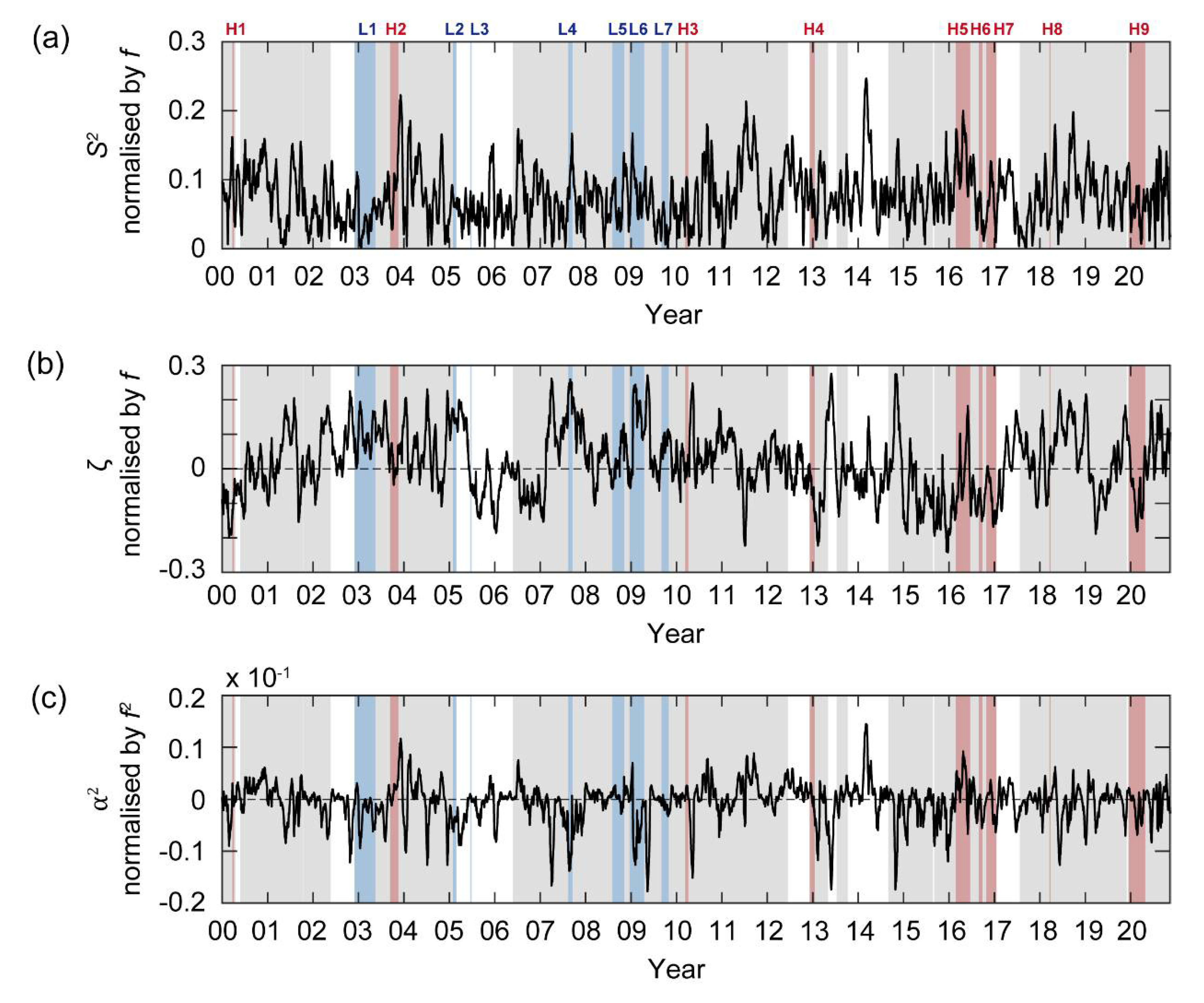
3.1. Intraseasonal, Interannual, and Decadal Variations of Near-Inertial Kinetic Energy below and within the Surface Mixed Layer

The VAR_{NIW_obs_int} values showed significant intraseasonal, interannual, and decadal variations, rather than seasonal variations, from 2000 to 2020 (Figure 5 and Table 1 and Table 2). Notably, VAR_{NIW_obs_int} averaged over period high (red shaded box) was approximately 12 times higher than that of period neutral. During period low (blue shaded box), there was almost no VAR_{NIW_obs_int} variation at 400 m (<0.02 J²/m⁶). The NIW kinetic energy (square root of VAR_{NIW_obs_int}) averaged over period high was ~$1.1\times {10}^3$ J/m³, which is approximately 24 times higher than that over period low (~$4.7\times 10$ J/m³). Relatively high (>$5.8\times {10}^5$ J²/m⁶) annual mean values of VAR_{NIW_obs_int} were found in 2003, 2012–2013, 2016, and 2020, with the maximum value being observed in 2016 (with the peak value of $9.5\times {10}^5$ J²/m⁶ in 2016 corresponding to H5) (Figure 7b). In terms of decadal variations of VAR_{NIW_obs_int}, period high appeared more frequently in the 2010s than the 2000s, yielding a decadal mean of VAR_{NIW_obs_int} in the 2010s (~$8.3\times {10}^4$ J²/m⁶), significantly (95% confidence) higher than that in the 2000s (~$3.1\times {10}^5$ J²/m⁶).

Interestingly, the timing of the enhanced VAR_{NIW_model_int} did not match well with that of VAR_{NIW_obs_int} (Figure 7a and Figure 8d,e). A VAR_{NIW_model_int} (or amplitude of NIWs) value greater than $1.0\times {10}^4$ J²/m⁶ (~1 m/s) was found on 12 September 2003, 19 August 2004, and 3 September 2020 (green triangles in Figure 8d,e); notably, only the first date corresponded to period high (H2). H5 corresponded to the period when the value of VAR_{NIW_obs_int} was higher than that during H2; however, the wind energy input during H5 (~7 kJ/m²) was smaller than that during H2 (~31 kJ/m²) (Figure 7a and Figure 8c). Except for H2 and H5, the amplitudes of the modelled NIWs and VAR_{NIW_model_int} were less than 0.2 m/s and $2.0\times {10}^3$ J²/m, respectively. It is also interesting that there was a statistically significant difference in VAR_{NIW_model_int} before and after 2010, yielding a higher decadal mean of 4.8 $\times {10}^2$ J²/m⁶ in the 2000s than the $4.5\times {10}^2$ J²/m⁶ observed in the 2010s, in contrast to the observational results (higher decadal mean of VAR_{NIW_obs_int} in the 2010s; Figure 7b).

3.2. Composite Mean of Near-Inertial Kinetic Energy at 400 m Dependent on Mesoscale Condition

In our study, the magnitudes of $\mathsf{\Pi }$ and $S^2$ composited for period high (period low) were significantly larger (smaller) than those for period neutral, showing $1.54\times {10}^{-3}$ W/m² ($0.43\times {10}^{-3}$ W/m²) and 0.08 f/s (0.06 f/s), respectively (Figure 8 and Figure 9 and Table 1 and Table 2). The $\mathsf{\Pi }$ during the period high events (except for H1 and H8) were significantly larger than the composite mean during period neutral, while those during period low events (except L6) were significantly smaller than those during period neutral. The ${\alpha }^2$ and $\zeta$ composite mean values for period high (period low) had positive (negative) and negative (positive) signs, showing $+2.80\times {10}^{-12}$/s² ($-20.45\times {10}^{-12}$/s²) and −0.04 f/s (0.10 f/s), indicating the dominance of strain to vorticity (vorticity to strain) and lower (higher) $f_{eff}$, respectively. At period high, it was shown that the $\zeta <0$ or strain fields were strengthened by mesoscale flow fields, while at period low, $\zeta >0$ by cyclonic circulation appeared (Figure 6). More than half of the period high and period low events could be identified by the signs of $\zeta$ and ${\alpha }^2$. The role of the $\zeta$ was identified by comparing Categories I and III for $S^2>{\zeta }^2$ (corresponding to ${\alpha }^2>0$), and Categories II and VI for $S^2<{\zeta }^2$ (corresponding to ${\alpha }^2<0$), commonly yielding more period high events for a negative $\zeta$ (Table 3). The role of $S^2$ was determined by comparisons between Categories I and II for $\zeta >0$ and between Categories III and IV for $\zeta <0$, commonly yielding more period high events for $S^2>{\zeta }^2$ (positive ${\alpha }^2)$. For each Category, the composite means of VAR_{NIW_obs_int} were $1.05\times {10}^5$, $1.29\times {10}^5$, $1.25\times {10}^5$, and $1.43\times {10}^5$ J²/m⁶ yielding that at Category I < Category II, Category III < Category < IV and Category II < Category IV with 95% significant level (p-value < 0.05). There was no significantly high correlation between Category II and Category III (p-value > 0.05).

4. Discussion

4.1. Comparison to Known Characteristics of Near-Inertial Internal Waves (NIWs)

We compared the results of nonseasonal variations of the observed and modelled NIW kinetic energy (VAR_{NIW_obs_int}) with previously known characteristics of NIWs. In general, period high often corresponded to the condition of $\zeta <0$ (Category III or IV), supporting that NIWs are trapped in a region of $\zeta <0$ because of the lowered $f_{eff}$ due to mesoscale circulations, as suggested in previous studies [37,38]. The interannual variations in the region of $\zeta <0$ imposed by the meandering of the subpolar front and the activities of anticyclonic eddies off the east coast of Korea may be responsible for the interannual variations of NIW kinetic energy presented in [38] and the horizontal and vertical distributions of NIW kinetic energy shown in [37]. The NIWs presented in [39,59] under the condition of $\zeta >0$ corresponded to Categories I or II in our study. Notably, significant impacts of $S^2$ on the NIW kinetic energy in the region have not been reported previously, except for a study conducted by Noh and Nam [40], which suggested a strong case of NIWs extracting their energy from a mesoscale flow field under the favourable condition of $S^2>{\zeta }^2$ (strain exceeds vorticity, ${\alpha }^2>0$) via the wave capture process [32,33]. The case found during events 2–4 in the study conducted by Noh and Nam [40], which supported the exponentially growing wavenumber, along with an increasing $S^2$ and a resulting small group velocity, corresponded to H2 in our study; this was generalised from statistically significant differences in the composite mean variance of NIW kinetic energy, for example, more period high events for $S^2>{\zeta }^2$.

Wind-induced NIWs are known to propagate downward below the MLD [37,60,61]. However, in spite of large $\mathsf{\Pi }$ values, only VAR_{NIW_model_int} (and not VAR_{NIW_obs_int}) showed an occasional enhancement, such as that observed on 19 August 2004 and 3 September 2020 (green triangles in Figure 8d), when the typhoon passed the region. This means that the nonseasonal variations in VAR_{NIW_obs_int} could not be well-explained by the changes in the surface wind forcing alone, additionally requiring the consideration of mesoscale field conditions. Another circumstantial energy source for NIWs in the deep layer in the region suggested by Mori et al. [36] is topographic roughness, because barotropic currents flowing over the rough bottom could generate deep near-inertial oscillations. Indeed, in this case, the current-topography interaction will also be affected by the mesoscale circulation, because the mesoscale eddies in the region are quasi-barotropic, as discussed in [39], which accounts for the higher NIW kinetic energy observed inside (where $\zeta <0$) the anticyclonic circulation in the region.

4.2. Effects of Surface Wind Forcing on Near-Inertial Energy within and below the Mixed Layer

The NIWs within the mixed layer can be easily amplified by the changes in the local wind stress; however, the wind-induced NIWs within or just below the mixed layer may dissipate mostly (up to 70–85%) in the upper 200 m [61,62,63], and hardly penetrate far below the MLD to 400 m depth, accounting for significantly different nonseasonal variations in the KE_{NIW_obs} at 400 m of the EC1 (VAR_{NIW_obs_int}) compared to those in KE_{NIW_model}, within the mixed layer simulated by the damped slab model using local wind stress (VAR_{NIW_model_int}). Positive anomalies of VAR_{NIW_model_int} exceeding $\mathsf{\sigma }+\mathsf{\mu } (~2.5\times {10}^3$ J²/m⁶) were not found during the events of period high, although they were clearly accompanied by relatively high $\mathsf{\Pi }$ values during H2 and H5 (Figure 7 and Figure 8). Indeed, periods of very high VAR_{NIW_model_int} (19 August 2004 and 3 September 2020) exceeding $1.0\times {10}^4$ J²/m⁶ in association with the passage of typhoons (Figure 2) corresponded to period neutral events indicative of only moderate VAR_{NIW_obs_int}. In general, VAR_{NIW_model_int} was low (less than $2.0\times {10}^3$ J²/m⁶) when $\mathsf{\Pi }$ decreased during period low. Significant dissipation of wind-induced NIWs may be confirmed around August 2004 (period neutral, green triangle in Figure 8); for example, the case when the KE_{NIW_obs} of $1.12\times {10}^2$ J/m³ observed at 400 m (corresponding to the square root of peak VAR_{NIW_obs_int} of $1.26\times {10}^4$ J²/m⁶) explained only 9.6% of the KE_{NIW_model} of ~$11.68\times {10}^2$ J/m³ within the mixed layer, supporting the deduction or strong dissipation of NIWs in the upper 200 m [62,63].

Because the surface wind stress is not uniform, equatorward- and downward-propagating NIWs generated by strong wind forcing in the north of EC1, despite the weak local wind forcing, may propagate down to 400 m of EC1, accounting for the high VAR_{NIW_obs_int} without a significant VAR_{NIW_model_int} (except H2 and H5). However, this possibility can be ruled out, as the intraseasonal variance in the kinetic energy of NIWs originating from higher latitudes (forced by wind stress at 38–40° N along the 131° E), propagating below the mixed layer to 400 m (of EC1; Figure 10), was not markedly different from VAR_{NIW_model_int}, nor did it correlate with VAR_{NIW_obs_int} (Figure 8e).

4.3. Effects of Mesoscale Flow Fields on Near-Inertial Energy Far below the Mixed Layer

The condition parameters of $\zeta$ and $S^2$ that represent the mesoscale flow field explained VAR_{NIW_obs_int} better than surface wind forcing, because a negative $\mathsf{\zeta }$ (Categories III and IV) lowers $f_{eff}$ (permitting the trapping and rapid deep propagation of NIWs) (Figure 6) [24,28] and increases $S^2$, leading to a positive anomaly of ${\alpha }^2$ (Categories I and III), which stretches and rotates the wavevector (resulting in exponentially growing wavenumber and decreasing group velocity), representing an enhancement of NIWs [30]. For example, the lowered $f_{eff}$ ($\zeta <0$) associated with the anticyclonic circulation around the EC1 supports the high VAR_{NIW_obs_int} during the H6, contrasting to the low VAR_{NIW_obs_int} during the L4 when $\zeta >0$, associated with the cyclonic circulation around the EC1 (Figure 6). During the two events (N1 and N2) of the neutral period, we observed low VAR_{NIW_obs_int} values despite high VAR_{NIW_model_int} values, in association with the typhoon passage, which may be explained by unfavourable conditions ($\zeta >0$ and $S^2<{\zeta }^2$; Category II) for NIW enhancement imposed by mesoscale conditions (Table 3). In contrast, more period high events were observed under favourable conditions ($\zeta <0$ and $S^2>{\zeta }^2$; Category III) for NIW enhancement imposed by mesoscale conditions (Table 3), mainly regardless of wind forcing.

The results of more frequent events of period high in the 2010s (compared to those in the 2000s) were also accounted for by the mesoscale field condition, and not by the surface-wind-induced NIWs within the mixed layer. The anticyclonic UWE anomalously lasted longer (nearly two years from October 2014 to August 2016) in the region [64], and a newly formed UWE appeared again in September 2016, providing mesoscale conditions of $\zeta <0$ that were favourable for NIW enhancement at 400 m of EC1 during H5, H6, and H7. Changes in mesoscale flow conditions due to the UWE in the 2010s accompanied the strengthening of density stratification in the region, yielding significantly higher $N$ and lower WKB scaling factor values at 400 m of EC1 during the 2010s, compared to those observed in the 2000s, due to a strong stratification linked to mesoscale conditions in 2003, 2006, 2011, 2013, and 2015–2018 (Figure 4). Interestingly, the 14% decrease in the WKB scaling factor or the increase in the NIW potential energy in the 2010s (compared to that observed in the 2000s), however, could not explain the increased frequency of period high events in the 2010s. Note that the events of period high and period low were not significantly dependent on whether WKB scaling was applied (now shown), indicating that the nonseasonal variation of NIW energy was more affected by the mesoscale flow field (vorticity and strain) than the stratification. The WKB scaling factor at 400 m was variable depending on the varying stratification, but always higher than the unity at the depth (Figure 3c–e and Figure 4b,d).

5. Concluding Remarks

Nonseasonal (intraseasonal, interannual, and decadal) variations in NIW kinetic energy, KE_{NIW_obs} at 400 m (VAR_{NIW_obs_int}) were presented from long time-series (from 2000 to 2020) moored observations in the southwestern East Sea. In total, nine periods of high (period high) and seven periods of low (period low) intraseasonal variance of KE_{NIW_obs}, or VAR_{NIW_obs_int} at 400 m, were identified and analysed statistically, providing composite means for different mesoscale conditions, and suggesting a significant effect of mesoscale flow fields on VAR_{NIW_obs_int}. Although a high rate of wind work, sometimes associated with typhoon passage, may significantly enhance the near-inertial kinetic energy (KE_{NIW_model} within or just below the surface mixed layer as simulated by the damped slab model), in our study, the intraseasonal variance of KE_{NIW_model}, or VAR_{NIW_model_int}, hardly accounted for VAR_{NIW_obs_int} at 400 m depth, which was dissipated mostly in the upper layer. Instead, the condition parameters of relative vorticity ($\zeta$) and the total strain ($S^2$), representing mesoscale flow fields, better explained VAR_{NIW_obs_int} at 400 m, yielding a significantly higher KE_{NIW_obs} at 400 m when $\zeta <0$ and/or $S^2>{\zeta }^2$, and vice versa (Figure 11). Our results, based on 21-year-long observations, statistically support previous (mostly theoretical) suggestions that NIW kinetic energy may have been enhanced through nonlinear interactions with the mesoscale flow field, when the strain exceeded the vorticity, and was trapped when the effective Coriolis frequency was lowered due to a negative relative vorticity. We believe that future process-oriented studies focusing on specific NIW events will provide a more comprehensive understanding of the interaction between the mesoscale flow fields and NIWs, testing the statistically derived proposition obtained in this study from rare, long-term, high-resolution, and continuous observations.

References

1. Garrett, C. What is the “near-inertial” band and why is it different from the rest of the internal wave spectrum? J. Phys. Oceanogr. 2001, 31, 962–971. [Google Scholar] [CrossRef]
2. Alford, M.H.; MacKinnon, J.A.; Simmons, H.L.; Nash, J.D. Near-inertial internal gravity waves in the ocean. Annu. Rev. Mar. Sci. 2016, 8, 95–123. [Google Scholar] [CrossRef] [Green Version]
3. MacKinnon, J.A.; Alford, M.H.; Ansong, J.K.; Arbic, B.K.; Barna, A.; Briegleb, B.P.; Bryan, F.O.; Buijsman, M.C.; Chassignet, E.P.; Danabasoglu, G.; et al. Climate process team on internal wave-driven ocean mixing. Bull. Am. Meteorol. Soc. 2017, 98, 2429–2454. [Google Scholar] [CrossRef] [PubMed] [Green Version]
4. Whalen, C.B.; MacKinnon, J.A.; Talley, L.D. Large-scale impacts of the mesoscale environment on mixing from wind-driven internal waves. Nat. Geosci. 2018, 11, 842–847. [Google Scholar] [CrossRef]
5. Egbert, G.D.; Ray, R.D. Significant dissipation of tidal energy in the deep ocean inferred from satellite altimeter data. Nature 2000, 405, 775–778. [Google Scholar] [CrossRef]
6. Nycander, J. Generation of internal waves in the deep ocean by tides. J. Geophys. Res. 2005, 110, C10028. [Google Scholar] [CrossRef] [Green Version]
7. Jiang, J.; Lu, Y.; Perrie, W. Estimating the energy flux from the wind to ocean inertial motions: The sensitivity to surface wind fields. Geophys. Res. Lett. 2005, 32, L15610. [Google Scholar] [CrossRef]
8. Garrett, C.J.R.; Munk, W. Internal waves in the ocean: A progress report. Annu. Rev. Fluid Mech. 1979, 11, 339–369. [Google Scholar] [CrossRef]
9. Munk, W.; Wunsch, C. Abyssal recipes II: Energetics of tidal and wind mixing. Deep-Sea Res. Part I Oceanogr. Res. Pap. 1998, 45, 1977–2010. [Google Scholar] [CrossRef]
10. Müller, P.; Briscoe, M. Diapycnal mixing and internal waves. Oceanography 2000, 13, 98–103. [Google Scholar] [CrossRef] [Green Version]
11. Alford, M.H. Redistribution of energy available for ocean mixing. Nature 2003, 428, 159–162. [Google Scholar] [CrossRef]
12. Ferrari, R.; Wunsch, C. Ocean circulation kinetic energy: Reservoirs, sources, and sinks. Annu. Rev. Fluid Mech. 2009, 41, 253–282. [Google Scholar] [CrossRef] [Green Version]
13. Whalen, C.B.; de Lavergne, C.; Naveira Garabato, A.C.; Klymak, J.M.; MacKinnon, J.A.; Sheen, K.L. Internal wave-driven mixing: Governing processes and consequences for climate. Nat. Rev. 2020, 1, 606–621. [Google Scholar] [CrossRef]
14. Nikurashin, M.; Ferrari, R. Overturning circulation driven by breaking internal waves in the deep ocean. Geophys. Res. Lett. 2013, 40, 3133–3137. [Google Scholar] [CrossRef]
15. Vic, C.; Garabato, A.C.N.; Green, J.M.; Waterhouse, A.F.; Zhao, Z.; Melet, A.; De Lavergne, C.; Buijsman, M.C.; Stephenson, G.R. Deep-ocean mixing driven by small-scale internal tides. Nat. Commun. 2019, 10, 2099. [Google Scholar] [CrossRef] [Green Version]
16. Blaker, A.T.; Hirschi, J.J.M.; Sinha, B.; de Cuevas, B.; Alderson, S.; Coward, A.; Madec, G. Large near-inertial oscillations of the Atlantic meridional overturning circulation. Ocean Model. 2012, 42, 50–56. [Google Scholar] [CrossRef]
17. Xiao, J.; Xie, Q.; Wang, D.; Yang, L.; Shu, Y.; Liu, C.; Chen, J.; Yao, J.; Chen, G. On the near-inertial variations of meridional overturning circulation in the South China Sea. Ocean Sci. 2016, 12, 335–344. [Google Scholar] [CrossRef] [Green Version]
18. Lucas, A.J.; Franks, P.J.S.; Dupont, C.L. Horizontal internal-tide fluxes support elevated phytoplankton productivity over the inner continental shelf. Limnol. Oceanog. 2011, 1, 56–74. [Google Scholar] [CrossRef]
19. Pan, X.; Wong, G.T.F.; Shiah, F.-K.; Ho, T.-Y. Enhancement of biological productivity by internal waves: Observations in the summertime in the northern South China Sea. J. Oceanogr. 2012, 68, 427–437. [Google Scholar] [CrossRef]
20. Muacho, S.; da Silva, J.C.B.; Brotas, V.; Oliveira, P.B. Effect of internal waves on near-surface chlorophyll concentration and primary production in the Nazaré Canyon (west of the Iberian Peninsula). Deep Sea Res. Part I Oceanogr. Res. Pap. 2013, 81, 89–96. [Google Scholar] [CrossRef]
21. Villamaña, M.; Mouriño-Carballido, B.; Marañón, E.; Cermeño, P.; Chouciño, P.; da Silva, J.C.B.; Díaz, P.A.; Fernández-Castro, B.; Gilcoto, M.; Graña, R.; et al. Role of internal waves on mixing, nutrient supply and phytoplankton community structure during spring and neap tides in the upwelling ecosystem of Ría de Vigo (NW Iberian Peninsula). Limnol. Oceanogr. 2017, 62, 1014–1030. [Google Scholar] [CrossRef]
22. Li, D.; Chou, W.C.; Shih, Y.Y.; Chen, G.Y.; Chang, Y.; Chow, C.H.; Lin, T.Y.; Hung, C.C. Elevated particulate organic carbon export flux induced by internal waves in the oligotrophic northern South China Sea. Sci. Rep. 2018, 8, 2042. [Google Scholar] [CrossRef] [PubMed] [Green Version]
23. Song, H.; Marshall, J.; Campin, J.M.; McGillicuddy, D.J. Impact of near-inertial waves on vertical mixing and air-sea CO2 fluxes in the Southern Ocean. J. Geophys. Res. Oceans 2019, 124, 4605–4617. [Google Scholar] [CrossRef] [Green Version]
24. Kunze, E. Near-Inertial Wave Propagation in geostrophic shear. J. Phys. Oceanogr. 1985, 15, 544–565. [Google Scholar] [CrossRef]
25. D’asaro, E.A. Upper-ocean inertial currents forced by a strong storm. Part III: Interaction of inertial currents and mesoscale eddies. J. Phys. Oceanogr. 1995, 25, 2953–2958. [Google Scholar] [CrossRef] [Green Version]
26. Whitt, D.B.; Thomas, L.N. Resonant generation and energetics of wind-forced near-inertial motions in a geostrophic flow. J. Phys. Oceanogr. 2015, 45, 181–208. [Google Scholar] [CrossRef]
27. Jing, Z.; Wu, L.; Ma, X. Energy exchange between the mesoscale oceanic eddies and wind-forced near-inertial oscillations. J. Phys. Oceanogr. 2017, 47, 721–733. [Google Scholar] [CrossRef]
28. Lee, D.-K.; Niiler, P.P. The inertial chimney: The near-inertial energy drainage from the ocean surface to the deep layer. J. Geophys. Res. Oceans 1998, 103, 7579–7591. [Google Scholar] [CrossRef]
29. Danioux, E.; Klein, P.; Rivière, P. Propagation of wind energy into the deep ocean through a fully turbulent mesoscale eddy field. J. Phys. Oceanogr. 2008, 38, 2224–2241. [Google Scholar] [CrossRef]
30. BÜhler, O.; McIntyre, M.E. Wave capture and wave–vortex duality. J. Fluid Mech. 2005, 534, 67–95. [Google Scholar] [CrossRef] [Green Version]
31. Polzin, K.L. Mesoscale eddy–internal wave coupling. Part I: Symmetry, wave Capture, and results from the mid-ocean dynamics experiment. J. Phys. Oceanogr. 2008, 38, 2556–2574. [Google Scholar] [CrossRef] [Green Version]
32. Polzin, K.L. Mesoscale eddy–internal wave coupling. Part II: Energetics and results from PolyMode. J. Phys. Oceanogr. 2010, 40, 789–801. [Google Scholar] [CrossRef]
33. Jing, Z.; Chang, P.; DiMarco, S.F.; Wu, L. Observed energy exchange between low-frequency flows and internal waves in the Gulf of Mexico. J. Phys. Oceanogr. 2018, 48, 995–1008. [Google Scholar] [CrossRef]
34. Chang, K.I.; Teague, W.J.; Lyu, S.J.; Perkins, H.T.; Lee, D.K.; Watts, D.R.; Kim, Y.B.; Mitchell, D.A.; Lee, C.M.; Kim, K. Circulation and currents in the southwestern East/Japan Sea: Overview and review. Prog. Oceanogr. 2004, 61, 105–156. [Google Scholar] [CrossRef]
35. Shin, H.-R.; Shin, C.-W.; Kim, C.; Byun, S.-K.; Hwang, S.-C. Movement and structural variation of warm eddy WE92 for three years in the Western East/Japan Sea. Deep Sea Res. Part II Top. Stud. Oceanogr. 2005, 52, 1742–1762. [Google Scholar] [CrossRef]
36. Mori, K.; Matsuno, T.; Senjyu, T. Seasonal/spatial variations of the near-inertial oscillations in the deep water of the Japan Sea. J. Oceanogr. 2005, 61, 761–773. [Google Scholar] [CrossRef]
37. Jeon, C.; Park, J.H.; Park, Y.G. Temporal and spatial variability of near-inertial waves in the East/Japan Sea from a high-resolution wind-forced ocean model. J. Geophys. Res. Oceans. 2019, 124, 6015–6029. [Google Scholar] [CrossRef]
38. Park, J.-H.; Watts, D.R. Near-inertial oscillations interacting with mesoscale circulation in the southwestern Japan/East Sea. Geophys. Res. Lett. 2005, 32, L10611. [Google Scholar] [CrossRef] [Green Version]
39. Byun, S.-S.; Park, J.J.; Chang, K.-I.; Schmitt, R.W. Observation of near-inertial wave reflections within the thermostad layer of an anticyclonic mesoscale eddy. Geophys. Res. Lett. 2010, 37, L01606. [Google Scholar] [CrossRef] [Green Version]
40. Noh, S.; Nam, S. Observations of enhanced internal waves in an area of strong mesoscale variability in the southwestern East Sea (Japan Sea). Sci. Rep. 2020, 10, 9068. [Google Scholar] [CrossRef] [PubMed]
41. Lee, H.; Nam, S. EC1, Long and Continuous Mooring Time Series from 1996 to 2020; SEANOE: Paris, France, 2021. [Google Scholar] [CrossRef]
42. Good, S.A.; Martin, M.J.; Rayner, N.A. EN4: Quality controlled ocean temperature and salinity profiles and monthly objective analyses with uncertainty estimates. J. Geophys. Res. Oceans 2013, 118, 6704–6716. [Google Scholar] [CrossRef]
43. Chelton, D.B.; DeSzoeke, R.A.; Schlax, M.G.; El Naggar, K.; Siwertz, N. Geographical variability of the first baroclinic Rossby radius of deformation. J. Phys. Oceanogr. 1998, 28, 433–460. [Google Scholar] [CrossRef]
44. Lim, S.; Jang, C.J.; Oh, I.S.; Park, J. Climatology of the mixed layer depth in the East/Japan Sea. J. Mar. Syst. 2012, 96–97, 1–14. [Google Scholar] [CrossRef]
45. Mulet, S.; Rio, M.H.; Etienne, H.; Artana, C.; Cancet, M.; Dibarboure, G.; Feng, H.; Husson, R.; Picot, N.; Provost, C.; et al. The new CNES-CLS18 global mean dynamic topography. Ocean Sci. 2021, 17, 789–808. [Google Scholar] [CrossRef]
46. U.S. Integrated Ocean Observing System. Manual for Real-Time Quality Control of In-Situ Current Observations; Version 2.1; U.S. Department of Commerce, National Oceanic and Atmospheric Administration, National Ocean Service, Integrated Ocean Observing System: Silver Spring, MD, USA, 2019. [CrossRef]
47. Min, Y.; Jeong, J.-Y.; Jang, C.J.; Lee, J.; Jeong, J.; Min, I.-K.; Shim, J.-S.; Kim, Y.S. Quality control of observed temperature time series from the Korea Ocean Research Stations: Preliminary application of ocean observation initiative’s approach and its limitation. Ocean Polar Res. 2020, 42, 195–210. [Google Scholar] [CrossRef]
48. Leaman, K.D.; Sanford, T.B. Vertical energy propagation of inertial waves: A vector spectral analysis of velocity profiles. J. Geophys. Res. 1975, 80, 1975–1978. [Google Scholar] [CrossRef]
49. Lee, K.; Nam, S.; Kim, Y.-G. Statistical characteristics of east sea mesoscale eddies detected, tracked, and grouped using satellite altimeter data from 1993 to 2017. Sea 2019, 24, 267–281. [Google Scholar] [CrossRef]
50. Torrence, C.; Compo, G.P. A practical guide to wavelet analysis. Bull. Am. Meteorol. Soc. 1998, 79, 61–78. [Google Scholar] [CrossRef] [Green Version]
51. de Boyer Montégut, C. Mixed layer depth over the global ocean: An examination of profile data and a profile-based climatology. J. Geophys. Res. 2004, 109, C12003. [Google Scholar] [CrossRef]
52. Pollard, R.T.; Millard Jr, R. Comparison between observed and simulated wind-generated inertial oscillations. Deep-Sea Res. Oceanogr. Abstr. 1970, 17, 813–816. [Google Scholar] [CrossRef]
53. D’Asaro, E.A. The energy flux from the wind to near-inertial motions in the surface mixed layer. J. Phys. Oceanogr. 1985, 15, 1043–1059. [Google Scholar] [CrossRef] [Green Version]
54. Park, J.J.; Kim, K.; Schmitt, R.W. Global distribution of the decay timescale of mixed layer inertial motions observed by satellite-tracked drifters. J. Geophys. Res. Oceans 2009, 114, C11010. [Google Scholar] [CrossRef] [Green Version]
55. Kawaguchi, Y.; Wagawa, T.; Igeta, Y. Near-inertial internal waves and multiple-inertial oscillations trapped by negative vorticity anomaly in the central Sea of Japan. Prog. Oceanogr. 2020, 181, 102240. [Google Scholar] [CrossRef]
56. Chiswell, S.M. Deep equatorward propagation of inertial oscillations. Geophys. Res. Lett. 2003, 30, 1533. [Google Scholar] [CrossRef]
57. Okubo, A. Horizontal dispersion of floatable particles in the vicinity of velocity singularities such as convergences. Deep-Sea Res. Oceanogr. Abstr. 1970, 17, 445–454. [Google Scholar] [CrossRef]
58. Chavanne, C.P.; Firing, E.; Ascani, F. Inertial oscillations in geostrophic flow: Is the inertial frequency shifted by ζ/2 or by ζ? J. Phys. Oceanogr. 2012, 42, 884–888. [Google Scholar] [CrossRef]
59. Shcherbina, A.Y.; Talley, L.D.; Firing, E.; Hacker, P. Near-surface frontal zone trapping and deep upward propagation of internal wave energy in the Japan/East Sea. J. Phys. Oceanogr. 2003, 33, 900–912. [Google Scholar] [CrossRef] [Green Version]
60. Song, H.; Jeon, C.; Chae, J.Y.; Lee, E.J.; Lee, K.N.; Takayama, K.; Choi, Y.; Park, J.H. Effects of typhoon and mesoscale eddy on generation and distribution of near-inertial wave energy in the East Sea. Sea 2020, 25, 55–66. [Google Scholar] [CrossRef]
61. Nam, S.; Kim, D.; Kim, H.R.; Kim, Y.G. Typhoon-induced, highly nonlinear internal solitary waves off the east coast of Korea. Geophys. Res. Lett. 2007, 34, L01607. [Google Scholar] [CrossRef] [Green Version]
62. Furuichi, N.; Hibiya, T.; Niwa, Y. Model-predicted distribution of wind-induced internal wave energy in the world’s oceans. J. Geophys. Res. Oceans 2008, 113, C09034. [Google Scholar] [CrossRef]
63. Zhai, X.; Greatbatch, R.J.; Eden, C.; Hibiya, T. On the loss of wind-induced near-inertial energy to turbulent mixing in the upper ocean. J. Phys. Oceanogr. 2009, 39, 3040–3045. [Google Scholar] [CrossRef]
64. Jin, H.; Park, Y.G.; Pak, G.; Kim, Y.H. On the persistence of warm eddies in the East Sea. Sea 2019, 24, 318–331. [Google Scholar] [CrossRef]
Figure 1. Schematics on interaction between mesoscale flow field (grey line) and wind-induced NIWs (red arrow), enhancing the near-inertial kinetic energy. Red spirals indicate dissipation of NIWs.
Jmse 10 00009 g001
Figure 2. Location of subsurface mooring EC1 (red square) with bathymetry (colour) in the southwestern East Sea, off the east coast of Korea. Green dotted line indicates meridional line where sea surface wind data were extracted. Black dashed lines indicate trajectories of typhoon Maemi in 2003, Megi in 2004, and Maysak in 2020. The yellow circles indicate radii of 30, 100 and 200 km centred at EC1, respectively.
Jmse 10 00009 g002
Figure 3. (a) Monthly mixed layer depth (MLD) estimated from EN4 (black line) data compared to that from Lim et al. [44] (yellow dot), (b) vertical structure of mean buoyancy frequencies, estimated from the EN4 data, at the upper 400 m nearby the EC1 mooring averaged over summer (June–July–August, red line) and winter (December–January–February, blue line) where the Nmax and MLD are remarked with circles and dashed horizontal lines with corresponding colours. Vertical dashed line in (b) indicates the depth-averaged reference N 0 ( 4.6 × 10 3 rad/s). Vertical profiles of (c) temperature, (d) buoyancy frequency and (e) WKB scaling factor observed using Argo floats located within 80 km from the EC1 (red, blue and orange lines were observed on 20 August 2014, 25 June 2015, and 23 December 2016, respectively.
Jmse 10 00009 g003
Figure 4. Time series of (a) monthly and (c) annual mean Buoyancy frequencies at 50 m (grey line, right y-axis in (a) only) and 400 m (black lines and squares, left y-axis) derived from EN4, (b) monthly and (d) annual mean Wentzel-Kramers-Brillouin (WKB) scale factors at 400 m. Dashed lines in (a,b) indicate temporal means for 400 m. Blue thick solid and thin dashed lines in (c,d) represent decadal means and their standard deviations for 2000s (from 2000 to 2010) and 2010s (from 2010 to 2020), respectively.
Jmse 10 00009 g004
Figure 5. Time series of (a) zonal ( u N I W ,   black line) and meridional ( v N I W , orange line) components of horizontal NIW oscillations, (b) KENIW_obs, (c) VARNIW_obs_int at 400 m in 2003 as an example. Red and blue shaded boxes and no shade in (c) indicate period high (H2), period low (L1), and period neutral, respectively. Red dashed line in (c) indicates σ + μ .
Jmse 10 00009 g005
Figure 6. One-month-long composite maps of geostrophic current (grey arrow) superimposed on rate of wind work Π (in colours) during the period high (27 August–26 September 2016, H6), period neutral (1–30 June 2011), and period low (1–31 August 2007, L4). Green square marker represents the EC1.
Jmse 10 00009 g006
Figure 7. (a) Time series of normalised intraseasonal variations in KENIW at 400 m (VARNIW_obs_int) from 2000 to 2020. Red (blue) shaded boxes indicate period high (period low) and grey shaded area indicates period neutral. White area represents the data gap (no data available). Events 2–4 in Noh and Nam [40] are marked at the top of H2 (pink). (b) Annual (squares) and decadal mean (blue thick lines) of VARNIW_obs_int. In (b), grey and white squares indicate annual mean values of years in which the data acquisition rate was more and less than 50%.
Jmse 10 00009 g007
Figure 8. Time series of (a) wind stress amplitude, (b) near-inertial band-passed zonal (red) and meridional (blue) wind stresses, (c) rate of wind work Π (left axis) and time integral of   Π showing cumulative wind energy input to the mixed layer (green solid line, right axis), (d) mixed layer near-inertial current amplitude, u M L 2 + v M L 2 , calculated from the damped slab model, and (e) intraseasonal-band variance of (d) from local (black) and remote (pink) wind stresses where the latter denotes wind stress averaged over 38–40° N. Red (blue) shaded boxes indicate period high (period low). Grey shaded area indicates period neutral. Green triangles in (ce) indicate the periods when the mixed layer near-inertial current amplitude was larger than 1 m/s.
Jmse 10 00009 g008
Figure 9. Time series of (a) S 2 normalised by f, (b) ζ normalised by f, and (c) α 2 normalised by f2. Red (blue) shaded boxes indicate period high (period low). Grey shaded area indicates period neutral.
Jmse 10 00009 g009
Figure 10. Ray path of near-inertial internal waves (NIWs) (thick, white, solid line) in the spatially varying stratification observed in March 2018 (H8). Yellow solid line indicates ray path that could reach the depth of 400 m at EC1 (yellow star). Background colour indicates potential temperature, and dashed line indicates isopycnals of 27, 28, and 29 kg/m3.
Jmse 10 00009 g010
Figure 11. Schematics of behaviour of near-inertial internal waves (NIW, red arrow) under mesoscale flow fields (streamlines, grey arrows) yielding different conditions of ζ and α 2 ; (a) Category I ( ζ > 0 and S 2 > ζ 2 ), (b) Category II ( ζ > 0 and S 2 < ζ 2 ), (c) Category III ( ζ < 0 and S 2 > ζ 2 ), and (d) Category IV ( ζ < 0 and S 2 < ζ 2 ). Different blue shading colours represent different isopycnal layers. Vertical scales of MLD and 400 m reference level are shown with thick grey arrows in the right bottom of (d).
Jmse 10 00009 g011