Article

Spatial Distribution and System Constraints Diagnosis of Medium- and Low-Yield Farmlands in Northern China Based on Remote Sensing


1
College of Water Conservancy Science and Engineering, Taiyuan University of Technology, Taiyuan 030024, China
2
Hebei Key Laboratory of Soil Ecology, Center for Agricultural Resources Research, Institute of Genetics and Developmental Biology, Chinese Academy of Sciences, Shijiazhuang 050021, China
3
College of Life Science, Hebei University, Baoding 071002, China
4
Hebei International Joint Research Center for Remote Sensing of Agricultural Drought Monitoring, School of Land Science and Space Planning, Hebei GEO University, Shijiazhuang 052161, China
*
Authors to whom correspondence should be addressed.
Agriculture 2026, 16(8), 896; https://doi.org/10.3390/agriculture16080896
Submission received: 4 March 2026 / Revised: 10 April 2026 / Accepted: 15 April 2026 / Published: 17 April 2026

Abstract

Accurately identifying medium- and low-yield farmlands (MLYF) and diagnosing their constraints are essential for targeted improvement of productivity and national food security. However, traditional evaluation is usually limited by coarse spatial resolution and high labor costs, and a methodological gap remains between large-scale MLYF classification and system constraints diagnosis. To address the current methodological gaps, this study developed a comprehensive framework to determine the spatial distribution of MLYF in northern China and clarify their key constraints. The framework combined the Spatio-Temporal Random Forest (STRF) algorithm with vegetation indices (VIs), climate, and soil data to delineate MLYF and uses interpretable machine learning to diagnose major constraints. The model showed high explanatory power and ensured the reliability of attribution results. The results showed that MLYF exhibited obvious spatial heterogeneity, accounting for 48.66% of the total cultivated land in the study area. These MLYF are primarily concentrated in the northwestern Loess Plateau (LP), the central Along the Great Wall (ATGW) region, and the peripheries of the Huang-Huai-Hai (HHH) Plain. In addition to spatial classification, our analysis revealed significant differences in constraint mechanisms: soil structural, nutrient, and salinization constraints predominantly restrict productivity in the HHH Plain, whereas water stress and soil erosion are the primary drivers of yield gaps in the LP and ATGW regions. These findings provide new data and insights for understanding the spatial heterogeneity of farmland quality in typical dryland agricultural regions in northern China, and offer a scientific basis for targeted land improvement and regional agricultural sustainability.

1. Introduction

For decades, food security has remained a major challenge in China, especially with increasing climate uncertainty and resource constraints. The continuous population growth and rising food demand have brought unprecedented pressure on agriculture and natural resources [1]. Farmland is the basis of grain production. Since the reserve of uncultivated farmland is almost exhausted, the strategic focus of agricultural development has inevitably shifted from expanding farmland area to improving land quality [1,2]. In this case, medium- and low-yield farmlands (MLYF) have become the key reserve for increasing yield, because they are widely distributed and have great potential for productivity improvement [3]. However, little is known about the spatial distribution and constraints of MLYF in the typical dryland agricultural regions in northern China. Therefore, the accurate identification and targeted improvement of MLYF are essential prerequisites for implementing the “sustainable development” strategy and ensuring national food security and meeting strategic development needs [4,5].
Traditionally, classification and evaluation of MLYF mainly rely on local statistical yield data and soil-based field surveys [4,6]. Although these methods provide the necessary baseline information, they are limited by coarse spatial resolution, high costs, and labor-intensive processes. Therefore, these methods are insufficient for capturing temporal dynamics and are difficult to extend to large-scale agricultural management [5,6]. With the rapid development of earth observation technology, remote sensing (RS) has become a powerful tool for large-scale crop monitoring. Remote sensing has been widely used to monitor crop growth, assess crop health, manage land resources and predict agricultural yield [7]. For example, multi-temporal vegetation indices (VIs) and phenological indicators have been proven effective in characterizing the productivity of cultivated land under different environmental gradients [8]. By combining phenological information with various remote sensing-derived parameters, robust yield prediction models have been developed for major crops such as maize and wheat [9,10]. In addition, the combination of multi-source remote sensing data and advanced machine learning algorithms can significantly improve the accuracy of yield prediction, especially in the vast arid and semi-arid areas [11]. However, relatively few studies have examined the relationship between the spatial distribution of MLYF and the diagnosis of yield constraint factors. Most studies based on remote sensing focus on maximizing the accuracy of yield estimates, while largely ignoring how environmental constraints affect the productive potential of farmland. This issue is particularly critical in dryland agriculture, where the dominant constraint factors may change rapidly between soil characteristics and climate variables. In addition, traditional diagnostic methods still rely heavily on static soil surveys, which often fail to capture the dynamic interaction between soil conditions and climate variability. Therefore, there remains a substantial methodological gap between yield prediction and production limit diagnosis, and few studies integrate these two aspects into a unified high-resolution framework. For the dryland agricultural areas in northern China, it is particularly urgent to address these gaps.
The typical dryland agricultural region in northern China has a wide geographical range and significant environmental gradient, in which the response of crops to climate and soil factors shows pronounced spatial heterogeneity [12,13]. Under such complex conditions, traditional global regression models and traditional machine learning algorithms usually show suboptimal prediction accuracy, because they often assume a unified and stable relationship in the entire study area. This oversimplification obscures important local variations and may lead to significant forecast deviations in specific areas [14,15,16]. In order to solve these limitations, this study adopted the Spatio-Temporal Random Forest (STRF) algorithm. STRF combines spatiotemporal weighting coefficients to capture local nonlinear relationships and considers the interannual fluctuations of environmental drivers, thus enhancing the sensitivity of the model to local changes [17,18]. This framework can more effectively represent complex nonlinear interactions and spatiotemporal characteristic patterns, thus supporting the accurate prediction of agricultural productivity in large heterogeneous environmental regions. In turn, the generated high-resolution prediction output provides a solid data basis for the description of MLYF and the identification of its key constraints.
To address the above research gaps, this study integrated 20 indicators, including vegetation indices (NDVI and EVI), climate variables and soil characteristics and developed a high-resolution agricultural productivity model for typical dryland agricultural regions in northern China using the STRF algorithm. This framework goes beyond traditional yield estimation by establishing a comprehensive framework that simultaneously maps the spatial distribution of MLYF and diagnoses their key constraints. The specific goals are: (1) to construct robust productivity prediction models for major crops and establish a systematic monitoring framework for MLYF; (2) to reveal the spatial distribution pattern of MLYF in northern dryland agricultural areas; (3) to determine the main constraints of MLYF and analyze its spatial heterogeneity within the study area. These findings are expected to provide a reliable scientific basis for agricultural improvement and for promoting sustainable agricultural development in the region.

2. Materials and Methods

2.1. Study Area

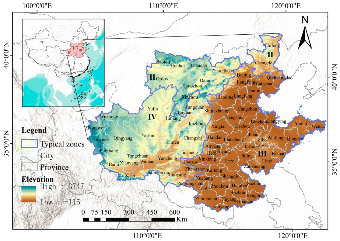
The study area extends from 104.63° E longitude to 123.27° E longitude, and from 30.92° N latitude to 40.82° N latitude, encompassing 744 counties. The study area (Figure 1) includes the Huang-Huai-Hai Plain (HHH), the Loess Plateau (LP), and the Along the Great Wall (ATGW) region. In general, these regions constitute the typical dryland agricultural areas in northern China. Agriculture in these regions is dominated by dryland farming, with winter wheat and maize being the main staple crops. The region has a temperate monsoon climate, with an average annual temperature ranging from 12 °C to 16 °C. The annual precipitation decreases from about 800 mm in the southeast to about 350 mm in the northwest. The growing season of wheat lasts approximately 8 months, from the end of September to mid-June of the following year [19], while the growth period of maize (mainly summer maize) is approximately 5 months, usually from mid-June to early October [20].

2.2. Data Sources

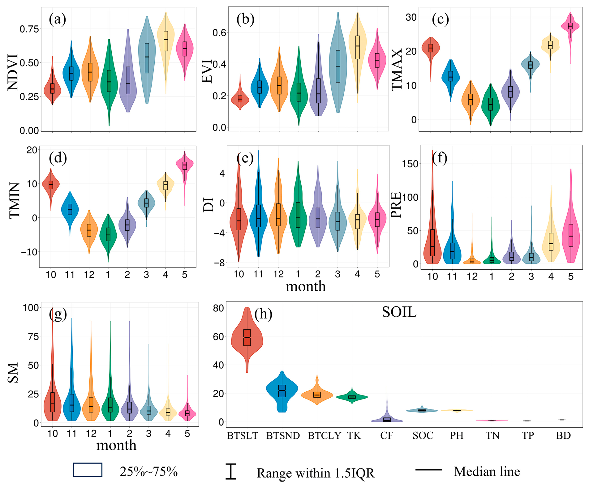
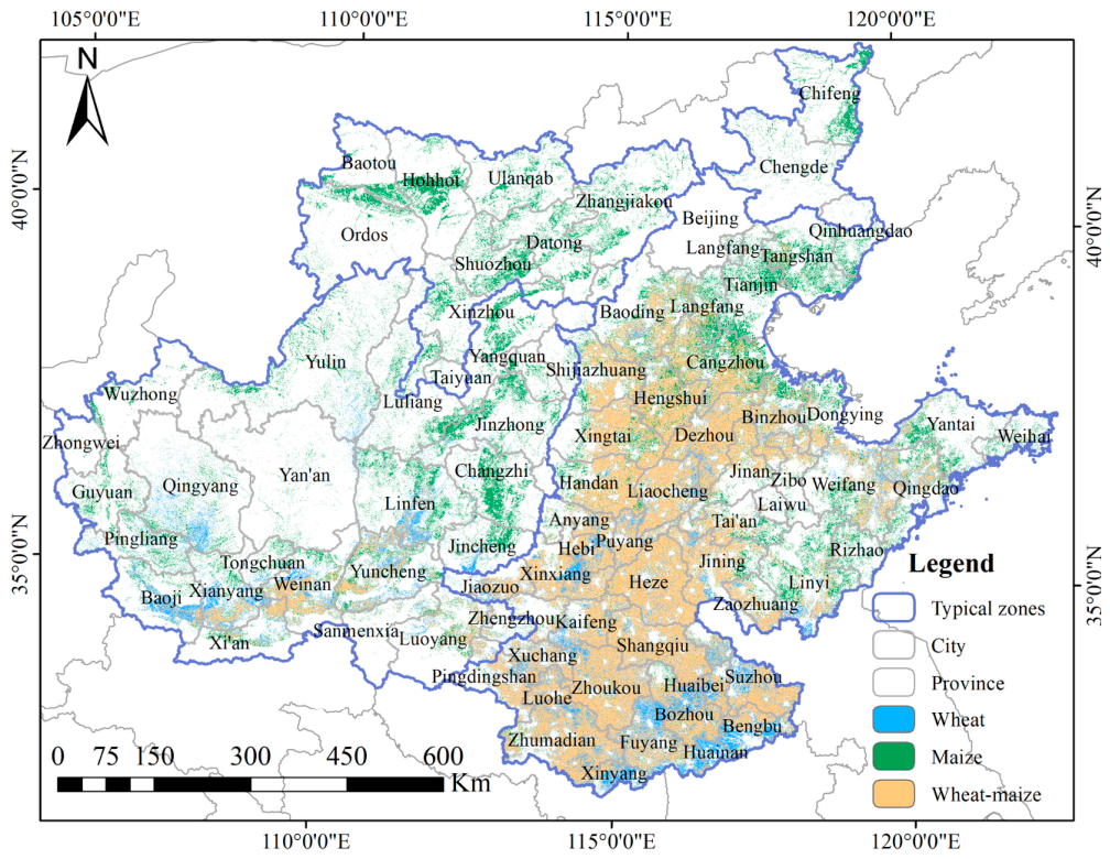
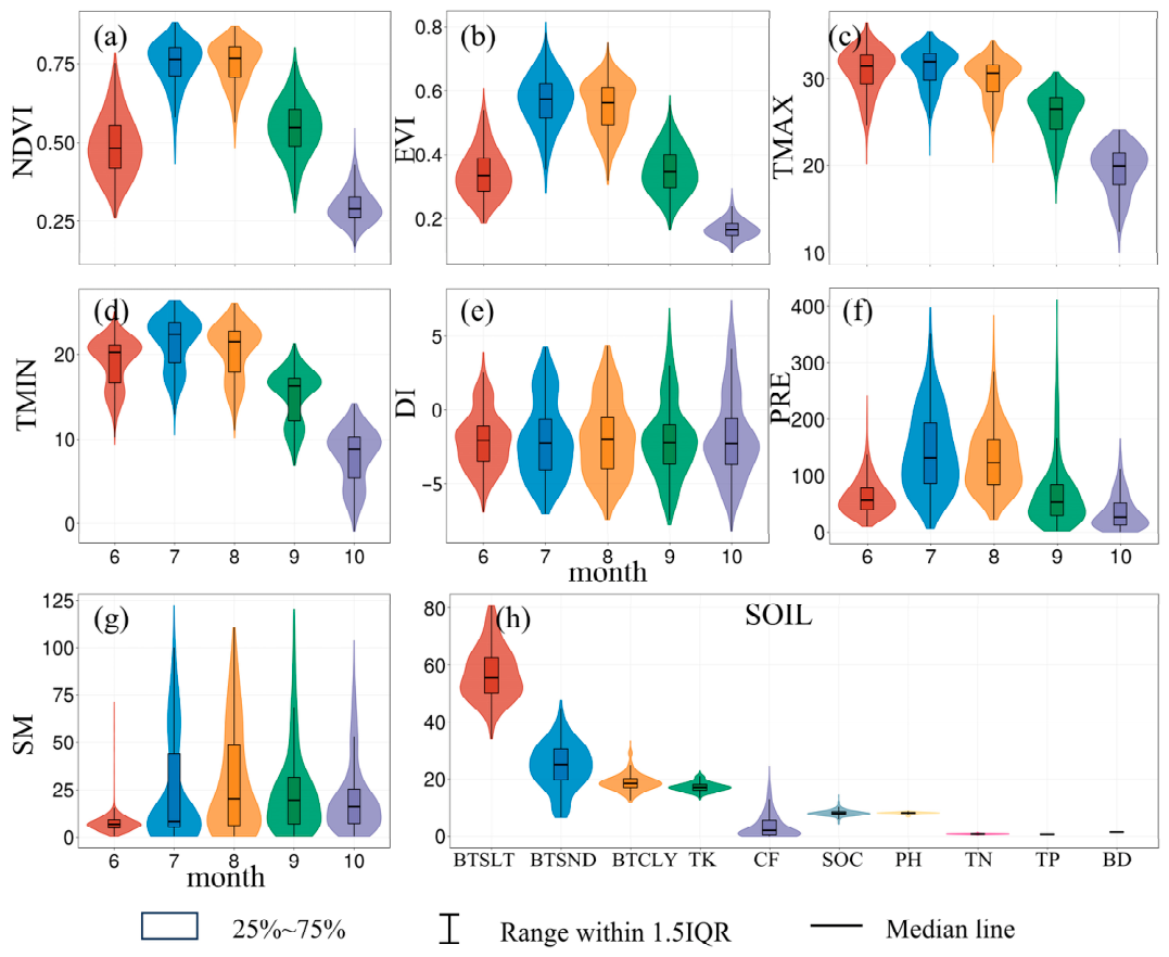
This study integrates multiple datasets from 2013 to 2024, including remote sensing indices, climate data, soil data, and crop yield statistics (available from 2013 to 2022). Table A1 (Appendix A) provides detailed information on the data sources and variables. The data processing workflow consisted of three main steps: First, all datasets were resampled to a unified spatial resolution of 250 m and aggregated to a monthly time scale. This step was mainly intended to ensure the spatial consistency of remote sensing, climate, soil and crop distribution datasets during cropland masking and subsequent spatial extraction. For categorical data (crop distribution masks), the majority resampling method was used to minimize the impact of mixed pixels, while for continuous variables (such as climate variables and remote sensing indices), bilinear interpolation was adopted to preserve spatial continuity. Second, the spatial distribution maps of major crops (maize and wheat) were used to mask all variables to exclude non-farmland pixels [21,22]. Third, the average values of all valid pixels within each county were calculated to obtain the county-level dataset for model training. Additionally, based on phenological information from the Crop Development Monitoring Platform of the China Meteorological Administration (https://www.nmc.cn/ accessed on 28 April 2025) and regional agronomic literature [13,23], crop-specific model training time windows were defined for each crop (see Table A2 in Appendix A). Data processing was mainly carried out using ArcGIS 10.7 and the MODIS Reprojection Tool (MRT). The spatial distribution of the predictor variables is shown in Figure 2 and Figure A1, and the spatial distribution of the crops is shown in Figure 3.
Data cleaning was carried out in two steps. First, the county-level average production over multiple years and its standard deviation (SD) were calculated, and samples outside the range of mean ± 3SD were removed to eliminate outliers [13,24]. Secondly, the county-level sown area derived from remote sensing was compared with that reported in the statistical yearbook; samples with differences greater than ± 35% were excluded to ensure data quality [21]. Specifically, in order to improve the accuracy of this comparison, the county-level cultivated land area of each crop was directly calculated from the original 30 m map.
These variables were divided into three groups [13]: (1) Remote sensing indices, including normalized difference vegetation index (NDVI) and enhanced vegetation index (EVI), were used to characterize the growth vitality and photosynthetic capacity of crops. (2) Climate factors include monthly maximum temperature (TMAX), monthly minimum temperature (TMIN), monthly cumulative precipitation (PRE), Palmer drought severity index (DI) and soil moisture (SM), which were used to explain the water balance and water and heat stress in the growing season. (3) Soil and topographic characteristics, including total nitrogen (TN), total phosphorus (TP), total potassium (TK), soil organic carbon (SOC), pH, gravel concentration (CF), texture (sand: BTSND; silt: BTSLT; clay: BTCLY), bulk density (BD), cation exchange capacity (CEC), electrical conductivity (EC) and soil erosion (ERO). These variables represent internal land quality attributes and constraints that determine long-term productivity patterns.

2.3. Research Framework

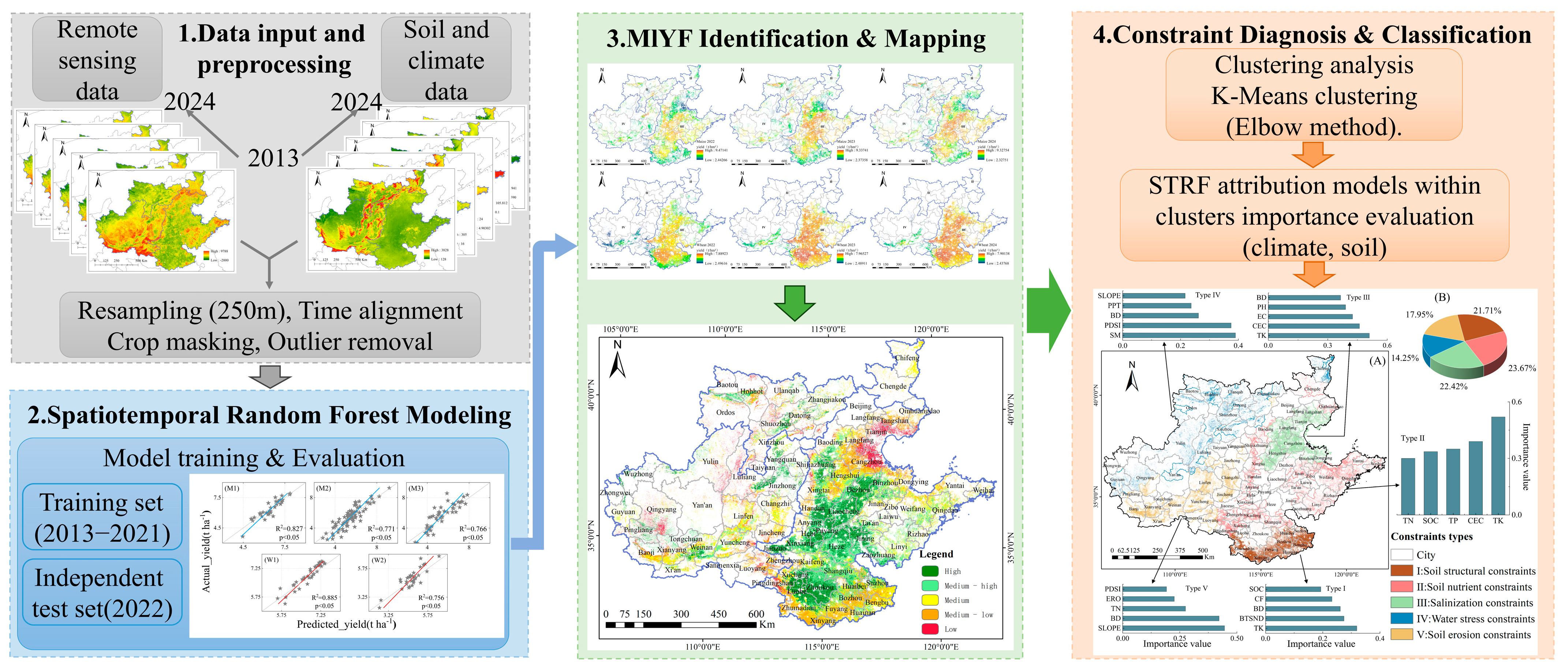
This study integrated remote sensing, soil, and climate datasets to develop a crop yield estimation framework based on the STRF algorithm. The workflow consisted of four sequential modules (Figure 4): (1) multi-source data preprocessing; (2) crop yield modeling and pixel-level yield mapping using STRF; (3) MLYF delineation based on regional yield benchmarks; and (4) dominant constraint diagnosis using K-means clustering and interpretable machine learning. Specifically, the optimized STRF model was used to generate high-resolution, multi-year yield grid maps for the study area. Based on the average annual yield, the farmland was divided into five productivity grades to describe the spatial distribution pattern of MLYF. Then, K-means clustering and an interpretable STRF classification model were jointly used to classify MLYF into different types and to quantify the relative importance of soil and climate factors in each cluster, thereby identifying the main constraints on MLYF formation. The analysis framework was designed to systematically reveal the spatial distribution of MLYF and its main constraints, and provide a scientific basis for precision agriculture and land improvement strategies. Because official statistical yield data were unavailable for 2023 and 2024, model calibration was based on data from 2013 to 2022, and the trained model was subsequently used to predict yields for 2023 and 2024.
The STRF algorithm was used to develop the crop yield production forecast model. The STRF algorithm is realized through the local weighting process to address the spatiotemporal non-stationarity of crop yield [17,18]. The core of this method is to establish a specific prediction model for each spatial location. The calculation process consists of the following sequential steps. Firstly, neighboring observations were selected as local training samples for each target location according to the spatiotemporal weight coefficient. Subsequently, the local random forest model was independently trained using a weighted dataset [18]. This mechanism allows the model to give priority to geographically close and temporally adjacent sample information, so as to capture local changes in the relationship between environmental drivers and yield [17]. In addition, STRF provides a measure of the importance of intrinsic variables, providing insights into the interpretation and selection of features [25]. Static soil variables were used to represent the stable spatial heterogeneity of baseline land quality, whereas dynamic remote sensing and climate variables were employed to capture interannual variations in crop growth and environmental conditions under different soil backgrounds. For model development, the dataset was divided chronologically: data from 2013 to 2021 were used as the training set, and the data from 2022 were retained as an independent test set. The model hyperparameters, including the number of decision trees, the maximum tree depth, the minimum number of samples required for splitting nodes, and the temporal weight coefficients, were optimized using a 5-fold cross-validation strategy on the training dataset [18,25,26]. During hyperparameter tuning, the training data of each crop-specific regional model were randomly divided into five approximately equal folds; in each iteration, four folds were used for model fitting, and one fold was used for validation. Specifically, after data cleaning, the full dataset from 2013 to 2022 contained 2591 valid county-level samples for maize and 1973 for wheat. This setup enables the model to capture the complex temporal and spatial relationship between environmental variables and crop yield, and the retention set verifies its time transferability. Before model training, all input variables were normalized. This algorithm was implemented in Python 3.12.
The performance of the final model was evaluated using the independent time-delay dataset from 2022. Three statistical indicators were used to quantify the prediction accuracy: the coefficient of determination (R2), root mean square error (RMSE), and mean absolute error (MAE) [27,28]. Higher R2 values indicate better model performance, whereas lower RMSE and MAE values denote smaller discrepancies between observed and predicted yields. Because RMSE and MAE are scale-dependent metrics, no universal fixed cutoff can be applied across different crops and regions. Therefore, model acceptability in this study was assessed comprehensively, based on relatively high R2 values, RMSE and MAE values that were low compared with the observed yield magnitude and agreement with the performance range reported in previous county-scale crop yield prediction studies. The corresponding formulas are as follows:
R 2 = 1 ( y i f i ) 2 ( y i y ¯ ) 2
R M S E = 1 n i = 1 n ( y i f i ) 2
M A E = 1 n i = 1 n | y i f i |
where n (i = 1,2,3……, n) is the total number of samples; y i is the observed crop yield; f i is the predicted crop yield and y ¯ is the mean of observed yield.
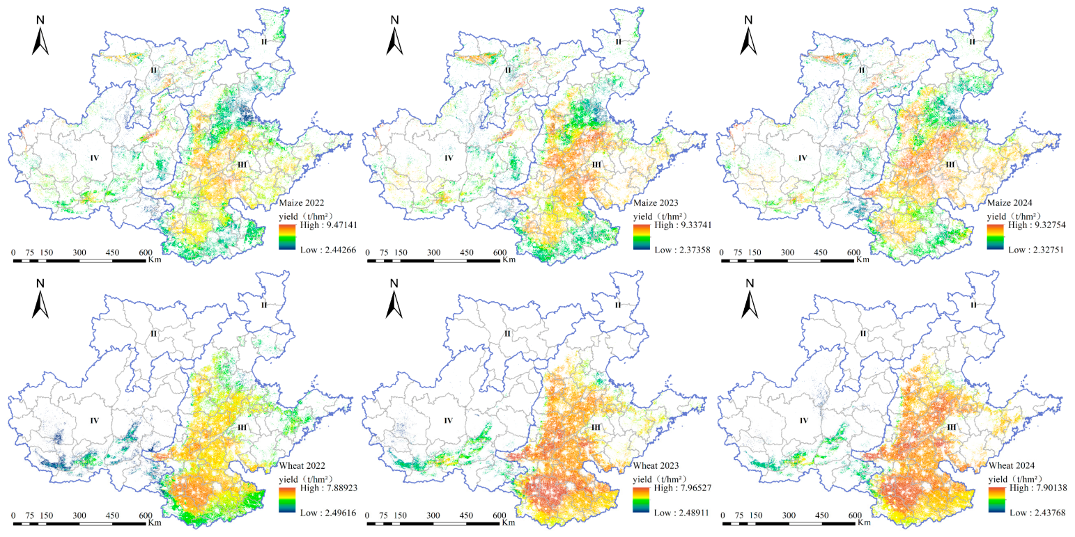
To depict the latest productivity model, the final determined STRF model (modeled using data from 2013 to 2022) was applied to the environmental variables from 2022 to 2024 to predict pixel-level yields. Due to the lack of official statistics for 2023 and 2024, the yields for the two years were estimated using remote sensing indices and meteorological data. The resulting spatial distribution is shown in Figure A2 in Appendix A. Then, the annual yield predictions from 2022 to 2024 were averaged to generate a three-year average agricultural productivity map, which serves as the baseline for the MLYF classification. Classification was performed using yield-based indicators as they directly represent the actual or potential productivity per unit area [29,30]. According to established criteria [31,32,33], MLYF classification standards were specified for each agricultural area, and the thresholds for MLYF are shown in Table 1. To quantify regional differences, the average productivity grade (APG) was further calculated. In this study, MLYF was formally defined as the combined area of medium-yield, medium-low-yield, and low-yield categories.
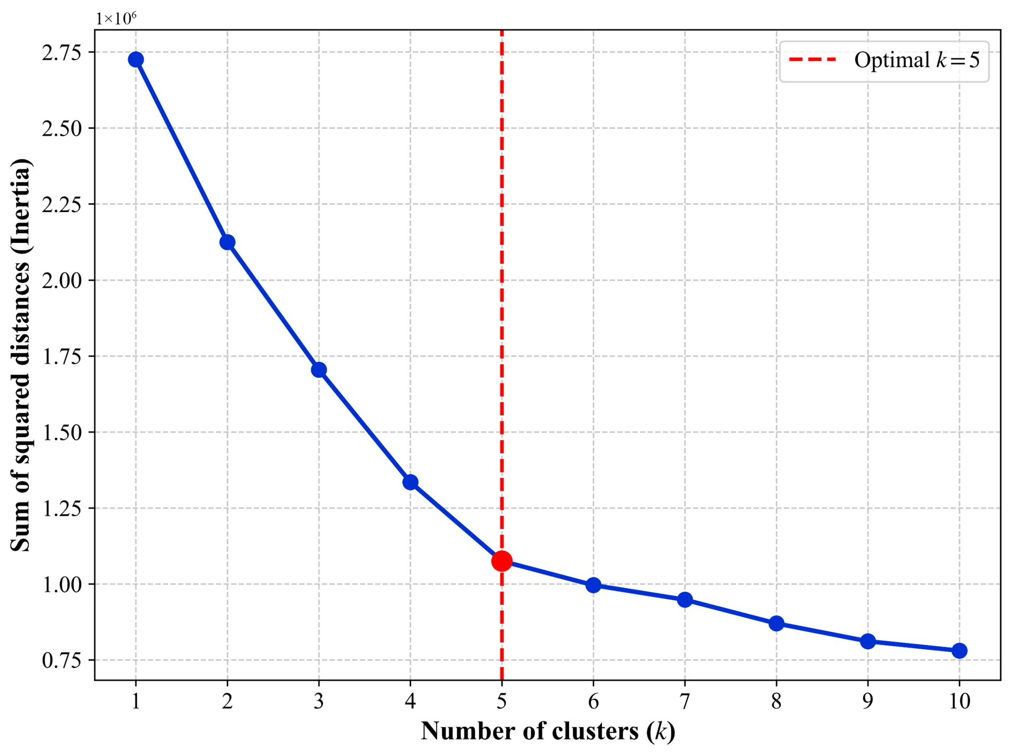
The formation of MLYF is usually controlled by multiple interacting factors, with climate and soil playing the main roles. The main constraints vary by region [5,34]. To systematically diagnose these constraints, this study developed an analytical framework, where K-means clustering was used for initial stratification, and the STRF algorithm was used for subsequent factor identification. First, based on the 3-year average predicted crop yield raster map generated in the previous step, 12,060 representative pixel-level samples were randomly extracted exclusively from the identified MLYF areas. Second, K-means clustering was applied to these sample points, using the predicted crop yield together with multidimensional climate and soil variables to stratify MLYF into environmentally similar groups. Before clustering, the optimal number of clusters was determined using the elbow method, which indicated an inflection point at K = 5 (Figure A5 in Appendix A). Finally, an interpretable STRF classification model suitable for these clusters was used to diagnose constraints by taking climate, soil and terrain variables as independent features. At this stage, vegetation indices were deliberately excluded to focus on internal environmental constraints (such as soil characteristics and topography) and climate drivers. The slope, soil conductivity, cation exchange capacity and other auxiliary indicators were introduced to enhance the discriminant ability of the model. By evaluating the feature importance within these localized interpretable models, the primary constraints limiting productivity were quantitatively determined.

3. Results

3.1. Yield Prediction Model Performance Evaluation

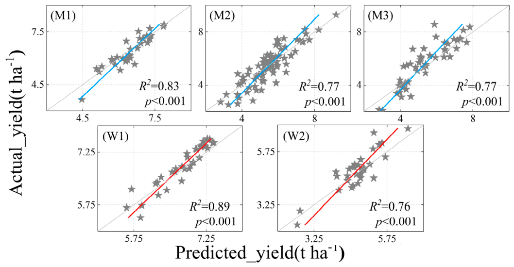
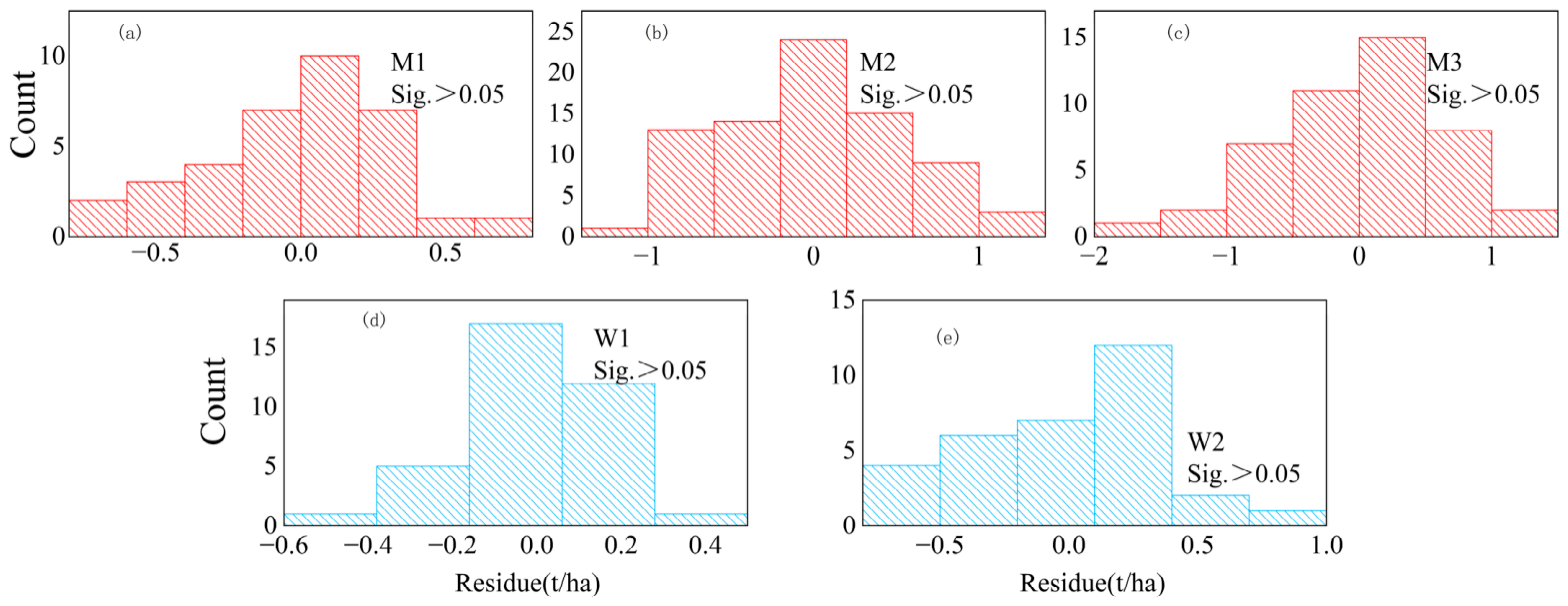
The performance of the final STRF model was comprehensively evaluated. The model residuals approximately followed a normal distribution and passed the Kolmogorov–Smirnov test (Figure A4 in Appendix A) to support the statistical validity of the regression model. Data from 2022 were used as an independent test set to further evaluate the accuracy of the model. The overall performance indicators are shown in Figure 5, and the specific parameters are shown in Table A2 (Appendix A).
The predicted output showed strong linear consistency with the observed value (R2 > 0.75), indicating high prediction accuracy. The performance in the HHH region was the best, with an R2 value of 0.89 for wheat and 0.83 for maize. The LP region also showed stable performance (R2 for wheat = 0.76, R2 for maize = 0.77). In the ATGW region, the R2 of the maize model was 0.77. Although this value was slightly lower, possibly due to the smaller planting area and sample size in this region, it still indicates satisfactory predictive ability. Additionally, the RMSE and MAE values for all typical agricultural areas were low (Table A2 in Appendix A), verifying the effectiveness and robustness of the STRF model for large-scale yield prediction in dryland agricultural regions. Therefore, the yield estimates generated in this study are applicable to characterizing the level of farmland productivity and provide a reliable data basis for subsequent MLYF identification.
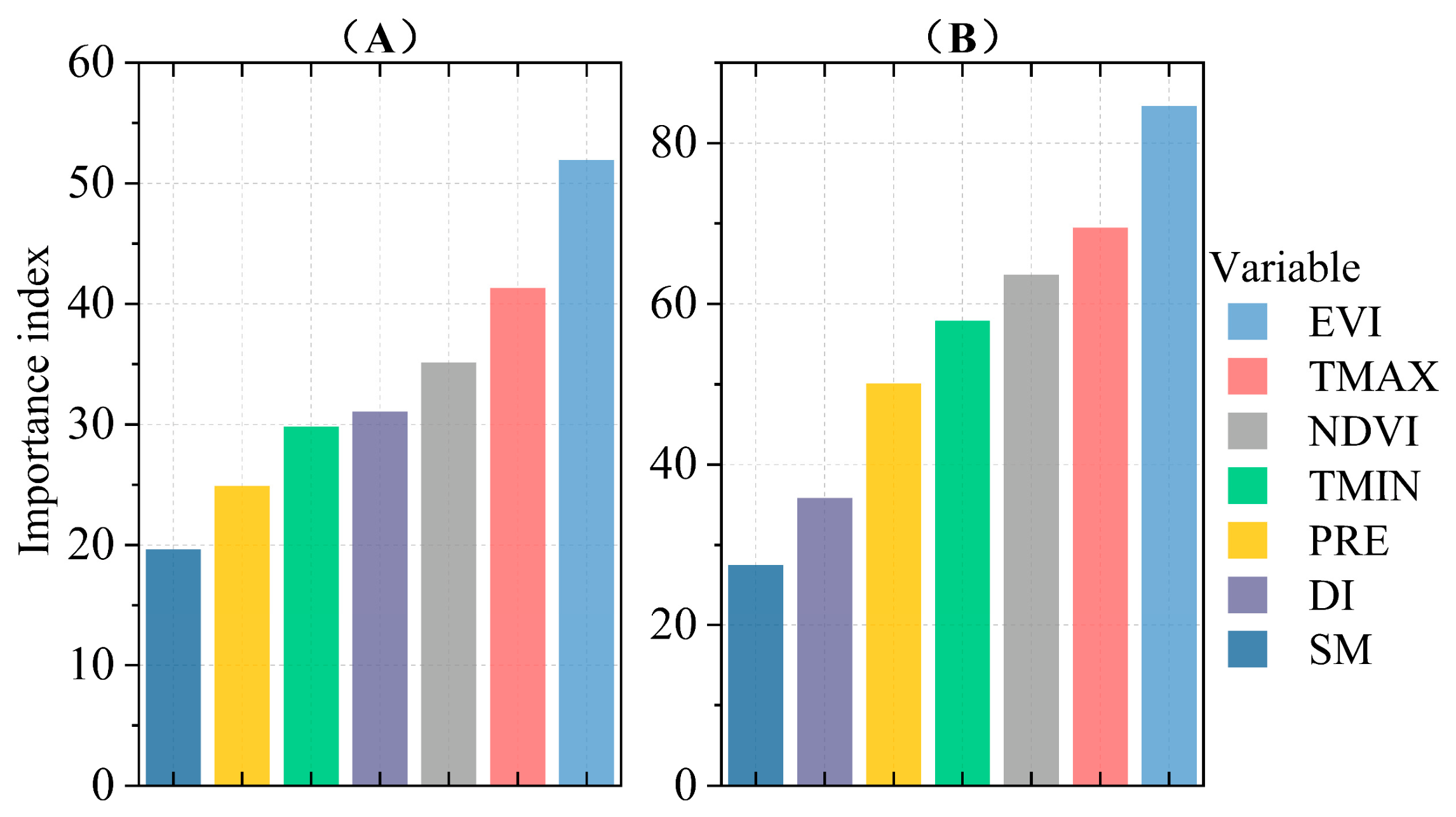
The relative importance of predictor variables for cropland productivity was quantified using the STRF model. Since STRF generates local variable importance for each spatial unit, global importance measures are derived by averaging these local importance values across the entire study area. The specific analysis focused on dynamic inputs—mainly time series remote sensing indices and meteorological data to capture seasonal growth patterns, while 10 static soil attributes were excluded to avoid potential confounding from temporally invariant factors. In order to facilitate the comparison between forecast variables, the importance value of each variable is summarized by adding the contributions of all time steps (months) of each variable in the growing season. The importance ranking of wheat was: EVI > TMAX > NDVI > DI > TMIN > PRE > SM (Figure 6A). For maize, EVI > TMAX > NDVI > TMIN > PRE > DI > SM (Figure 6B). These results emphasize the key role of VIs in crop yield prediction, in which EVI is more important than NDVI. Among the climate variables, temperature and precipitation also contribute greatly to the model performance.

3.2. MLYF Distribution Characteristics

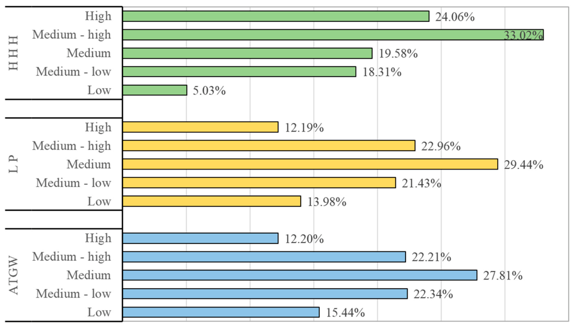
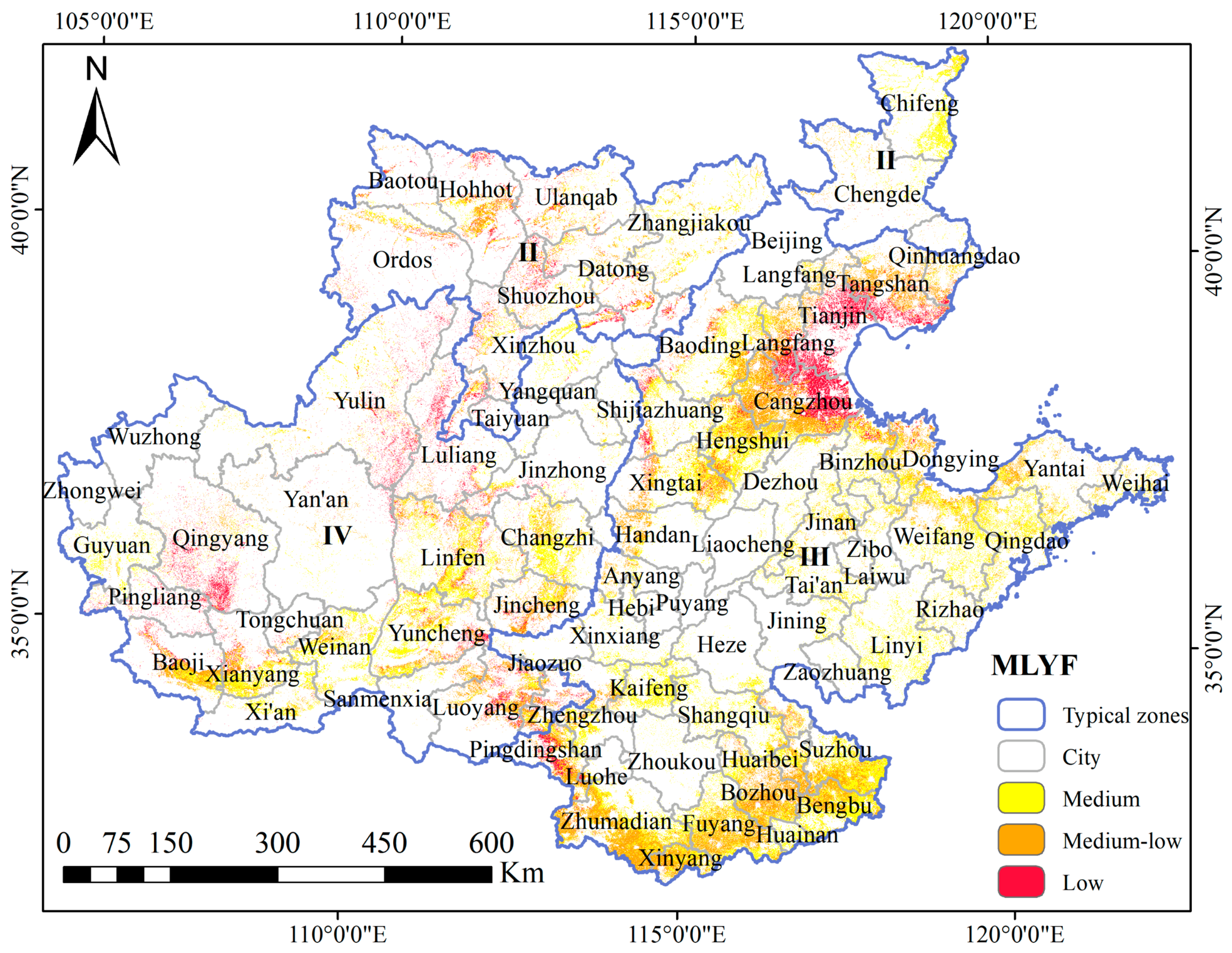
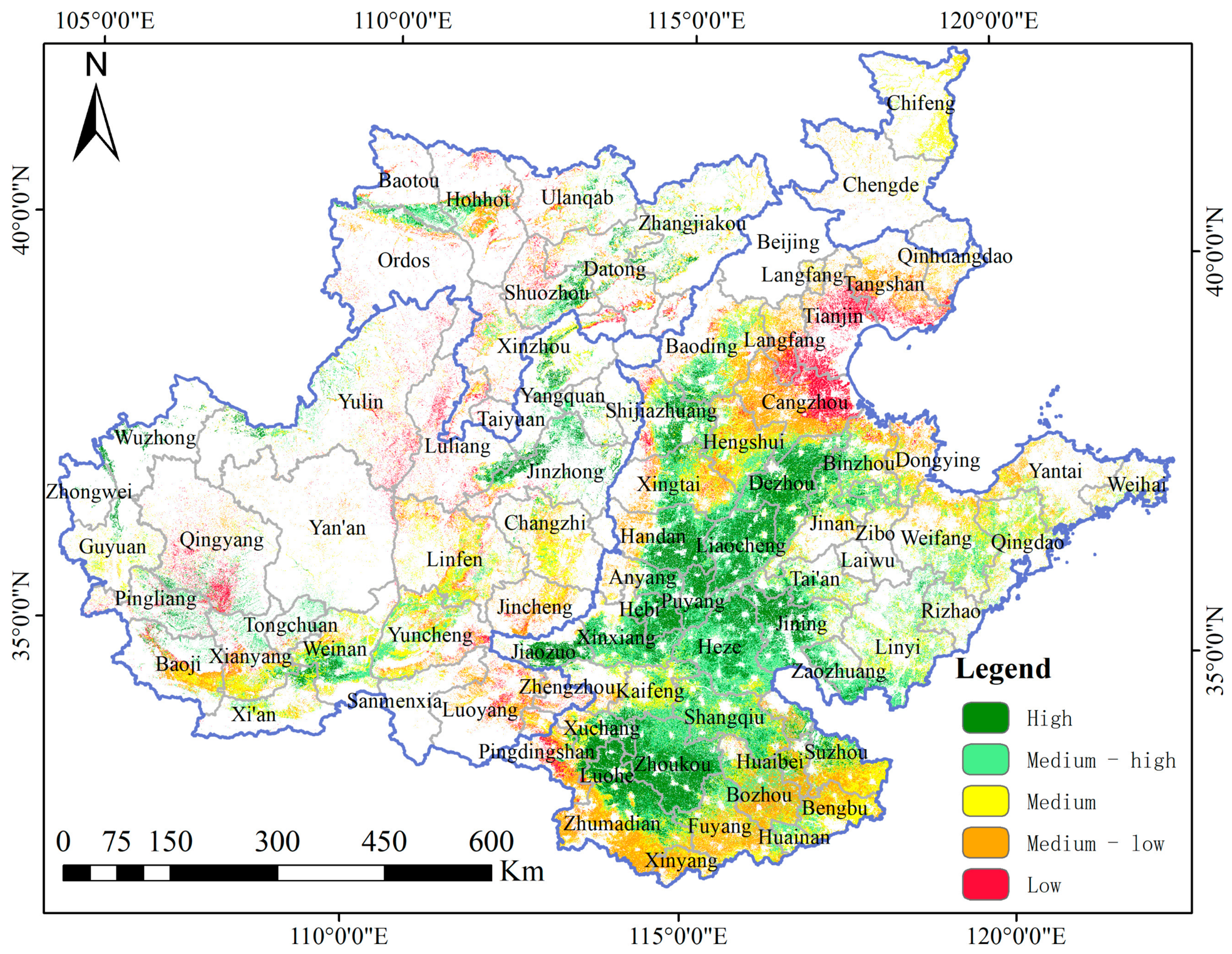
Based on the three-year average yield (2022–2024), the spatial distribution of MLYF was delineated. At the regional scale, the proportion of five cropland productivity grades in the typical dryland agricultural regions in northern China was as follows: high yield (20.98%), medium-high yield (30.36%), medium yield (22.02%), medium-low yield (19.18%) and low yield (7.46%) (Figure 7). MLYF was widely distributed, mainly in the northwest LP, the middle of ATGW and the northern and southern edges of HHH. Figure 8 illustrates the distribution of MLYF in the study area. The comprehensive distribution of the five productivity grades is shown in Appendix A, Figure A3.
The regional statistics further revealed significant regional heterogeneity: the total sown area in the HHH region was 2.01 million ha, and the average productivity grade (APG) was 2.47; MLYF accounted for 42.92% of the area, concentrated primarily in the northeastern and southern regions. The LP region covered 0.51 million ha, with an APG of 3.12; MLYF accounts for 64.85% of its area, mainly concentrated in hilly and gully areas in northwest China. The total sown area of ATGW was 0.19 million ha, with an APG of 3.17; MLYF accounts for 65.59% of its area, mainly distributed along the southern and northern foothills of the Yinshan Mountains (Figure 8).

3.3. Dominant Constraint Factors and Spatial Distribution of MLYF

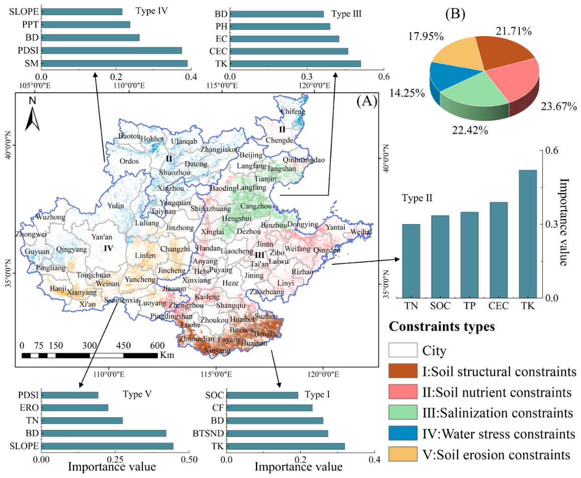
According to the dominant environmental constraints, MLYF in the study area can be classified into five main constraint types: (1) soil structure constraint; (2) soil nutrient constraint; (3) salinization constraint; (4) water stress constraint, and (5) soil erosion constraint. These categories showed clear regional aggregation and spatial heterogeneity in northern China (Figure 9). The attribution models showed strong explanatory performance, supporting the interpretability of the identified constraint types.
In the HHH region, the distribution of MLYF was mainly affected by a gradient of soil constraint. Soil structural constraints driven by physical properties such as BTSND, BD and CF were mainly concentrated in the south of HHH. Across the plain, soil nutrient constraints became the dominant factor, characterized by the lack of TK, SOC and CEC. In the northern coastal areas and specific inland areas, the dominant constraints shifted toward salinization, which is manifested by the increase in pH value and EC level. In contrast, the LP and ATGW regions are characterized by a transition from soil-based to climate-driven and topographic constraints. In the northwest LP and ATGW regions, water resource pressure was the dominant constraint, and productivity is mainly affected by SM, DI and PRE. At the same time, the south LP was mainly constrained by soil erosion, which is characterized by terrain and erodibility indicators, especially slope and ERO. In general, these findings reveal the obvious spatial heterogeneity of MLYF formation, with productivity controlled by environmental bottlenecks in specific regions.

4. Discussion

4.1. Model Performance and Methodological Applicability in Agricultural Systems

This study developed a reliable research framework to identify MLYF by establishing a high-resolution farmland productivity model. Driven by the integration of multi-source climate, remote sensing and soil datasets, the STRF algorithm achieved consistently high prediction accuracy in all agricultural regions (R2 > 0.75 in all cases), highlighting its robust ability to depict the spatial distribution of agricultural productivity. Although the performance of ATGW is relatively low (R2 = 0.77), this difference is mainly due to the obvious landscape fragmentation and relatively limited sample size in this area. Compared with previous studies, the STRF-based approach showed substantially better performance. For example, Zhang et al. [35] reported that they employed regression analysis and obtained an R2 range of 0.54 to 0.64, while Cheng et al. [36], who used standard random forest to obtain R2 values of approximately 0.66. The method based on STRF shows a significant performance leap. By capturing large-scale spatial nonstationary, the framework is particularly suitable for simulating agricultural productivity in regions with complex terrain and climate change characteristics. The results show that the model has high prediction accuracy, which provides a reliable basis for accurate identification of MLYF spatial patterns and subsequent implementation of site-based land management strategy.
The high predictive accuracy of the STRF model in this study is mainly attributed to three methodological advantages. Firstly, this model integrates vegetation indices, climate variables, and soil data, capturing both short-term crop growth signals and long-term environmental regulatory factors. Secondly, STRF explicitly considers the non-stability of space-time by giving greater weight to adjacent spatial-temporal observation data, thereby reducing the deviation caused by global parameter assumptions. The refinement of this method effectively captures the key features in a specific space-time neighborhood [17,18], thus enhancing the sensitivity of the model to complex nonlinear relationships. Thirdly, the implementation of a regional zoning modeling strategy has successfully alleviated the confusion effect caused by phenological differences in different regions and different planting systems [25,37]. Furthermore, an independent test using 2022 data further confirmed the time transferability of this model.
The importance analysis of prediction variables confirmed the complex and diverse effects of different variables on crop growth and yield, which is consistent with previous understanding [38]. Remote sensing VIs, such as NDVI and EVI, can effectively characterize the physiological characteristics of crops at different growth stages [5,38], especially at flowering and filling stages [39]. The study found that the correlation between VIs and yield was usually weak in the early growth period, when climate factors often provide more prediction information. On the contrary, the comprehensive effect of climate variables and the significant contribution of VIs in the late growth period are crucial to the robust yield prediction. This study combines multi-temporal VIs with climate data to estimate yield more accurately, thus improving the accuracy of MLYF classification. However, it is worth noting that machine learning methods have inherent limitations in mechanism interpretability.

4.2. Spatial Pattern of MLYF

This study systematically revealed the spatial distribution characteristics of cultivated land productivity and MLYF in the typical dryland agricultural regions in North China from 2022 to 2024 (Figure A2 and Figure 8). The distribution of MLYF shows obvious environmental zoning, which is determined by the synergy between regional natural conditions and agricultural management practices. Based on the productivity model of STRF and the analysis of the importance of variables, this study provides a mechanism interpretation for the driving factors of these spatial patterns.
MLYF exhibits marked spatial heterogeneity in the north and south edges of HHH and scattered inland areas. As shown in Figure 9, the main constraints in the north of HHH (especially in the east of Hebei) were CEC, EC, and pH, which are closely related to soil salinization. The increase in pH value and EC values of surface soil indicates that the concentration of soluble salt is high, which confirms the existence of salinization. This situation produces physiological stress on crops, inhibits the absorption of water and nutrients [40,41,42] and ultimately inhibits farmland productivity. This finding is consistent with Li et al. [43], who believe that salinization is the main obstacle to agricultural production in northern coastal areas. In the southern HHH, the dominant constraints include BTSND, BD and CF, reflecting the poor physical structure. These conditions induce nutritional stress in the key phenological period, thus hindering the realization of yield potential. On the contrary, in the middle and east of HHH, nutrition-related indicators are the highest, indicating that these areas are mainly restricted by soil fertility. The lack of SOC and TP leads to productivity gaps, which indicates that these intensive production areas need to transition to precise fertilization schemes. SOC is a fundamental driver of crop productivity; it not only acts as a primary reservoir for essential plant nutrients but also fundamentally improves soil aggregation, water-holding capacity, and aeration [44]. Therefore, despite favorable water conditions, the depletion of SOC severely limits the realization of yield potential in these intensive production areas.
In the northwestern LP and most areas of the ATGW, the concentrated distribution of MLYF is mainly driven by severe water stress. Our results show that SM, DI and PRE are the dominant factors. The data from these regions show that the persistent low SM and PRE and the long-term high DI reflect the persistent water deficit. As a key limiting factor [45], even under other optimal conditions, water shortage will hinder the increase of production, leading to extensive “water stress constraint” MLYF [46,47,48]. Traditionally, soil fertility rather than drought is considered to be the main bottleneck of crop yield in this area [49,50]. However, an important finding of this study is that water resource pressure has replaced soil fertility as the main limiting factor in these areas. This change shows that the recent farmland improvement policy has effectively alleviated the restrictions on soil fertility, and climate drought has gradually become the main constraint on productivity.
In the hilly and gully areas of LP and ATGW, topography and ERO are the core driving factors of cultivated land degradation and productivity decline. Severe erosion erodes the fertile topsoil, increases the sand content, and thins the effective soil depth, thus greatly reducing the water and nutrient retention capacity [51]. In addition to directly inhibiting soil productivity, these processes also hinder the development of root architecture, thus affecting the utilization efficiency of limited water and fertilizer resources [51,52]. Therefore, these restrictions eventually form “soil erosion type” MLYF, which is characterized by long-term low yield and unstable yield. This observation is consistent with Wang et al. [53], who pointed out that the soil and water loss caused by erosion seriously damaged the crop vitality and yield in the whole LP area.
To provide an indirect assessment of the plausibility of the productivity classification, the identified productivity levels were reclassified and compared with previously reported large-scale benchmarks. The resulting proportions for high, medium (Medium-High + Medium), and low-yields (Medium-Low + Low) were 20.98%, 52.38%, and 26.64%, respectively. These results are generally consistent with the historical data of cultivated land resources and their development and utilization in China (21.54% high yield) [54], and the evaluation based on NPP (20.66% high yield) [55]. It is worth noting that, compared with other methods, the proportion of middle yield fields in this research report is higher, and the proportion of low yield fields is correspondingly reduced. This difference can be attributed to the active implementation of land improvement policies aimed at restoring low-quality farmland. Although all methods capture the macro-scale regional pattern, the framework based on STRF provides superior spatial resolution and a more fine-grained representation of specific constraint types, promoting the paradigm shift from “all-inclusive” management to specific site intervention.

4.3. Implications for MLYF Improvement and Food Security

Based on the five main constraint categories identified in this study, we propose the following spatially differentiated repair strategies to enhance the productive potential of MLYF:
Solving soil structure constraints: Mainly distributed in the south of HHH, the main goal is to alleviate soil compaction and improve aeration under the intensive double cropping system. It is suggested to use mechanical subsoiling to break up the compaction plow pan caused by long-term rotary tillage [56]. At the same time, straw returning, especially wheat returning after harvest, is crucial to increase soil organic matter in these sandy loam landscapes and optimize soil porosity [57].
Optimize soil nutrient management: Distributed in the intensive production areas in the middle and east of HHH, the constraints usually come from nutrient imbalance rather than absolute lack. Management strategies should transition from traditional large-scale fertilization to precise fertilization programs. This requires the promotion of soil testing and balanced N-P-K fertilization [58], and at the same time, applying bio-organic fertilizers to stimulate soil microbial activity and thereby improve the nutrient utilization efficiency of these high-potential areas. This mechanism is important because soil physical and chemical properties, such as pH value, organic matter content and nutrient distribution, strongly influence the composition and function of bacterial communities [59].
Salinization mitigation: Concentrated in the northern coastal HHH and “Bohai granary” areas, restoration must be combined with engineering intervention and agronomic measures [60]. The basic hydraulic measures include the construction of a drainage network to reduce the groundwater level. These measures should be combined with agronomic measures, such as cultivating salt-tolerant crop varieties, applying soil amendments to replace exchangeable sodium ions, and slowing down secondary salinization [61].
Relieve water resources pressure: In response to irrigation water shortages in the northwest arid area and the ATGW area, water-saving agriculture should be prioritized. Major interventions include the widespread use of plastic mulch to suppress evapotranspiration and the deployment of rainwater harvesting systems, such as storage silos [48]. Giving priority to breeding drought-tolerant varieties and optimizing planting structure are crucial to stable yield. In areas where irrigation conditions permit, high-efficiency water-saving technologies such as drip irrigation, sprinkler irrigation, and under-mulch drip irrigation should also be promoted to improve water-use efficiency [62].
Control soil erosion: In the southern LP hilly and gully area, ecological restoration takes priority over agricultural intensification. We strongly advocate the strict implementation of the “green for food” policy. For areas with a slope of more than 25°, it is required to change farmland back to forests or grasslands. For cultivable gentle slopes, terrace works and soil conservation tillage technologies such as no tillage and contour tillage should be implemented to minimize surface runoff and reduce nutrient loss [63].
This interpretable diagnostic framework of machine learning has made significant progress compared with the traditional classification methods that only rely on the yield level. It has successfully linked the macro spatial distribution pattern with the underlying constraints mechanisms, thus facilitating a paradigm shift from the “one size fits all” extensive pattern to the precise implementation of the “local conditions” strategies in crop rotation management. Improving farmland fertility and releasing the productive potential of existing farmland are important ways to enhance China’s comprehensive grain production capacity and ensure national food security. This framework provides practical guidance for interventions tailored to local conditions and provides a solid scientific basis for formulating efficient farmland quality improvement policies at the regional level.

4.4. Uncertainties in the Study

This study is subject to several sources of uncertainty arising from both data limitations and methodological assumptions. An important limiting factor arises from data quality, especially the static nature of soil data, which cannot capture short-term changes caused by agricultural management practices. In addition, the relatively coarse spatial resolution of climate data may weaken the prediction ability of machine learning models, thus affecting the precision of yield estimation. In this study, all datasets were resampled to a uniform 250 m grid. Although the bilinear interpolation method can preserve the overall spatial continuity, it may smooth out local climate gradients, and this effect is particularly noticeable in complex terrain areas such as the LP and gullies. As a result, the fine-scale differences in temperature, precipitation, and drought conditions may be underestimated, thereby reducing the model’s ability to capture micro-scale yield heterogeneity. In addition, alternative approaches such as statistical downscaling or topographic correction may better preserve local climatic heterogeneity in complex terrain. However, because this study primarily aimed to achieve spatial harmonization across multi-source datasets at a large regional scale, these approaches were not implemented in the current framework. Future studies should further assess whether such methods can reduce interpolation-induced uncertainty. Another important limitation is the lack of direct pixel-level or county-level external validation of the final productivity classification. Although field management practices (such as irrigation, fertilization and variety selection) are crucial to crop growth [64], it is still a difficult challenge to systematically obtain such high-precision data in a wide geographical range. Although our model captures these overall effects indirectly through remote sensing and climate data, it cannot completely replace direct management information.
In terms of methodology, the current model involves inherent spatial and temporal uncertainties. Spatially, the scale mismatch between coarse county-level statistical data and high-resolution pixel-level predictor variables inevitably introduces uncertainty during data transformation. Temporally, the extrapolation of yield data for 2023 and 2024 carries the risk of larger prediction deviations, particularly if unprecedented climatic variations occurred during these unobserved years. Furthermore, although machine learning models show strong data mining capabilities, their “black box” architecture often lacks explicit representation of the internal physiological and ecological processes of crops. This lack of mechanistic interpretability may, to some extent, bring uncertainty to the model prediction under extreme or non-similar environmental conditions [65]. On the contrary, the process-based crop growth model is designed to simulate the biophysical development inside the crop. Therefore, the collaborative coupling of machine learning and mechanistic crop growth models provides a promising frontier for enhancing the robustness of future yield prediction [66].
Remote sensing data with higher spatial resolution (such as Sentinel-2) provides new opportunities for improving prediction accuracy [67]. In addition, new indicators, such as sun-induced chlorophyll fluorescence (SIF), provide a direct link to actual photosynthetic activity and are becoming an excellent alternative indicator for monitoring vegetation physiological status and instantaneous productivity [68]. Their potential in yield forecasting needs more rigorous exploration. Future research should focus on developing more robust diagnostic models that deeply integrate multi-source environmental data with advanced phenological physiological remote sensing indicators.

5. Conclusions

The MLYF of typical dryland agricultural regions of northern China were systematically identified using the STRF model, integrating multi-source data such as vegetation indices, climate and soil variables. The results show that MLYF accounts for 48.66% of the study area, with significant clustering in the northwestern LP, ATGW center, and the periphery of HHH. Through the interpretable diagnostic framework, we divided MLYF into five main constraint types: soil structure constraints, soil nutrient constraints, salinization constraints, water stress constraints and soil erosion constraints and proposed targeted management strategies for each type. The observed spatial pattern reflects the long-term interaction between physical factors and agricultural practices. The high yield stability of HHH arose from the coordinated adjustment of water, heat and soil resources, while the formation of MLYF was mainly driven by local environmental constraints. Finally, this study advocates the paradigm shift of farmland management from yield-centered classification to a diagnostic and cause-oriented framework, effectively bridging the gap between macro-scale remote sensing monitoring and micro-scale environmental driving. The proposed method provides an expandable blueprint for “accurate land management”, contributes to China’s food security, and provides a transferable approach for the sustainable intensification of the global dryland agricultural system.

Author Contributions

Conceptualization, Y.L., X.L. and X.S.; Methodology, Z.Z., X.L. and X.S.; Validation and investigation, X.S. and Z.T.; Data curation and original draft preparation, X.S.; Review and editing, X.S., X.L. and Z.Z.; Supervision, W.D., C.H., C.Z. and X.L.; Funding acquisition and project administration, X.L. All authors have read and agreed to the published version of the manuscript.

Funding

This research was supported by the National Key Research and Development Program of China (2022YFD1901604).

Data Availability Statement

The original contributions presented in the study are included in the article; further inquiries can be directed to the corresponding authors.

Acknowledgments

We sincerely express our gratitude for the support provided by the National Major Research and Development Program of China.

Conflicts of Interest

The authors declare no conflicts of interest.

Abbreviations

The following abbreviations are used in this manuscript:
MLYFMedium- and Low-Yield Farmlands
STRFSpatio-Temporal Random Forest
HHHHuang-Huai-Hai Plain
LPLoess Plateau
ATGWAlong the Great Wall
VIsVegetation Indices
NDVINormalized Difference Vegetation Index
EVIEnhanced Vegetation Index
SOCSoil Organic Carbon
TMIN Monthly Minimum Temperature
TMAX Monthly Maximum Temperature
PRE Accumulated Precipitation
DI Palmer Drought Severity Index
SM Monthly Soil Moisture
RFRandom Forest
RMSERoot Mean Square Error
MAEMean Absolute Error
RAY Regional Average Yield
APG Average Productivity Grade

Appendix A

Table A1. Data sources used in this study.
Data TypeVariableData IntroductionPeriodResolutionReference
Yield-Yield monitor
data (t ha−1)
YearRegionalNBS [69]
Cultivated land pixel-Maize/Wheat
maps
Year30 m × 30 mNational Ecosystem Science Data Center
[21,22,70]
Remote sensing dataNDVIMOD13Q116 days250 m × 250 mNASA LP
DAAC
EVIMOD13Q116 days250 m × 250 m
Meteorological dataTMAXunit: °CMonthly4 km × 4 kmTerra Climate [71]
TMINunit: °CMonthly4 km × 4 km
DI-Monthly4 km × 4 km
PREunit: mmMonthly4 km × 4 km
SMunit: mmMonthly4 km × 4 km
Soil dataTPunit: g kg−1-250 m × 250 mNational Ecosystem
Science Data Center [72,73]
TNunit: g kg−1-250 m × 250 m
TKunit: g kg−1-250 m × 250 m
SOCunit: g kg−1-250 m × 250 m
pH--250 m × 250 m
CFunit: % vol-250 m × 250 m
BDunit: g cm−3-250 m × 250 m
BTSLTunit: g kg−1-250 m × 250 m
BTCLYunit: g kg−1-250 m × 250 m
BTSNDunit: g kg−1-250 m × 250 m
CECunit: cmol (+) kg−1-250 m × 250 m
Supplementary
data
ECunit: mS cm−1-1 km × 1 kmHWSD [74]
EROunit: t (hm2 a)−1Year30 m × 30 mEarth System
Science Data [75]
NDVI: normalized difference vegetation index; EVI: enhanced vegetation index; TMAX: monthly maximum temperature; TMIN: monthly minimum temperature; DI: palmer drought severity index; PRE: monthly accumulated precipitation; SM: soil moisture; TP: total phosphorus content; TN: total nitrogen content; TK: total potassium content; SOC: soil organic carbon; pH: soil acidity; CF: gravel concentration; BTSND: sand concentration; BTSLT: silt concentration; BTCLY: clay particle; BD: soil bulk density; CEC: cation exchange capacity; EC: soil electrical conductivity; ERO: soil erosion.
Table A2. Hyperparameters and predictive performance of the STRF models.
Areas (Crop)Time WindowNumber of TreesMax DepthMin Samples LeafSpatiotemporal WeightRMSEMAER2
HHH (maize)6–101001050.300.380.290.83
LP (maize)6–101001050.100.680.540.77
ATGW (maize)5–101001050.250.830.620.77
HHH (wheat)10–51001050.300.240.210.89
LP (wheat)10–51001050.300.460.360.76
Time window, number of trees, max depth, min samples leaf, and neighbors count are all parameters of the STRF model; 10–5: The period from October to May of the following year.
Figure A1. The distribution of processed monthly parameter data for the period 2013–2024 (maize) is presented, including NDVI (a), EVI (b), TMAX (c), TMIN (d), DI (e), PRE (f), SM (g), as well as soil physicochemical properties (h). The numbers on the x-axis represent the respective months. NDVI: normalized difference vegetation index; EVI: enhanced vegetation index; TMAX: monthly maximum temperature; TMIN: monthly minimum temperature; DI: palmer drought severity index; PRE: monthly accumulated precipitation; SM: soil moisture; BTSLT: silt content; BTSND: sand content; BTCLY: clay content; TK: total potassium content; CF: gravel concentration; SOC: soil organic carbon content; PH: hydrogen ion concentration; TN: total nitrogen content; TP: total phosphorus content; BD: soil bulk density.
Agriculture 16 00896 g0a1
Figure A2. Distribution of crop productivity for wheat (top) and maize (bottom) in the study area across the three-year period 2022–2024 (II: Inner Mongolia and Along the Great Wall; III: Huang-Huai-Hai Plain; IV: Loess Plateau).
Agriculture 16 00896 g0a2
Figure A3. Distribution characteristics map of agricultural production capacity level in the typical dryland farming region of northern China.
Agriculture 16 00896 g0a3
Figure A4. Residual distribution plot of predicted yields from different models. The residual distribution of all models had passed the Kolmogorov–Smirnov test (Sig. > 0.05) and approximately followed a normal distribution. Letters (M) and (W) denote maize and wheat, respectively; Red and blue denote maize and wheat, respectively; numbers 1, 2, and 3 represent the HHH, LP, and ATGW, respectively; (ae) represents the model error distribution map for the agricultural area and crops.
Agriculture 16 00896 g0a4
Figure A5. Elbow curve for determining the optimal number of clusters for MLYF constraint diagnosis.
Agriculture 16 00896 g0a5

References

  1. Lu, Y.; Jenkins, A.; Ferrier, R.C.; Bailey, M.; Gordon, I.J.; Song, S.; Huang, J.; Jia, S.; Zhang, F.; Liu, X.; et al. Addressing China’s grand challenge of achieving food security while ensuring environmental sustainability. Sci. Adv. 2015, 1, e1400039. [Google Scholar] [CrossRef]
  2. Ministry of Agriculture of the People’s Republic of China. Report on the National Cultivated Land Quality Grade; Ministry of Agriculture of the People’s Republic of China: Beijing, China, 2015; Volume 136, pp. 58–64.
  3. Ministry of Agriculture of the People’s Republic of China. 2019 Report on the National Cultivated Land Quality Grade; Ministry of Agriculture of the People’s Republic of China: Beijing, China, 2020; Volume 199, pp. 113–121.
  4. Bai, X.; Zhang, J.; Cui, Z.; Wang, G.; Lu, Y.; Zhang, F. Advances in the Indicator and Assessment Approaches of Medium-low Yield Fields. Acta Pedol. Sin. 2023, 60, 913–924. [Google Scholar]
  5. Zhang, J.; Li, Y. Analysis of the Current Situation of Medium and Low Yield Fields in China. Front. Sustain. Dev. 2023, 3, 21–24. [Google Scholar] [CrossRef]
  6. NY/T 1634-2008; Technical Regulation for Cultivated Land Fertility Survey and Quality Assessment. Ministry of Agriculture of the People’s Republic of China: Beijing, China, 2008.
  7. Nandeha, N.; Trivedi, A.; Subhasish, B.; Chauhan, V.; Dange, M.M. A Review of Remote Sensing and GIS in Agronomic Decision-Making. Int. J. Environ. Clim. Change 2025, 15, 348–360. [Google Scholar] [CrossRef]
  8. Murakami, T.; Ogawa, S.; Ishitsuka, N.; Kumagai, K.; Saito, G. Crop discrimination with multitemporal SPOT/HRV data in the Saga Plains, Japan. Int. J. Remote Sens. 2001, 22, 1335–1348. [Google Scholar] [CrossRef]
  9. Hill, M.J.; Donald, G.E. Estimating spatio-temporal patterns of agricultural productivity in fragmented landscapes using AVHRR NDVI time series. Remote Sens. Environ. 2003, 84, 367–384. [Google Scholar] [CrossRef]
  10. Ji, Z.; Pan, Y.; Zhu, X.; Wang, J.; Li, Q. Prediction of Crop Yield Using Phenological Information Extracted from Remote Sensing Vegetation Index. Sensors 2021, 21, 1406. [Google Scholar] [CrossRef]
  11. Raza, A.; Shahid, M.A.; Zaman, M.; Miao, Y.; Huang, Y.; Safdar, M.; Maqbool, S.; Muhammad, N.E. Improving Wheat Yield Prediction with Multi-Source Remote Sensing Data and Machine Learning in Arid Regions. Remote Sens. 2025, 17, 774. [Google Scholar] [CrossRef]
  12. Zhao, Y.; Xiao, D.; Bai, H.; Tang, J.; Liu, D.L.; Qi, Y.; Shen, Y. The Prediction of Wheat Yield in the North China Plain by Coupling Crop Model with Machine Learning Algorithms. Agriculture 2022, 13, 99. [Google Scholar] [CrossRef]
  13. Han, J.; Zhang, Z.; Cao, J.; Luo, Y.; Zhang, L.; Li, Z.; Zhang, J. Prediction of Winter Wheat Yield Based on Multi-Source Data and Machine Learning in China. Remote Sens. 2020, 12, 236. [Google Scholar] [CrossRef]
  14. Li, X.H. Random forest is a specific algorithm, not omnipotent for all datasets. Chin. J. Appl. Entomol. 2019, 56, 170–179. [Google Scholar]
  15. Zhu, T. Analysis on the Applicability of the Random Forest. J. Phys. Conf. Ser. 2020, 1607, 12123. [Google Scholar] [CrossRef]
  16. Roustaei, N. Application and interpretation of linear-regression analysis. Med. Hypothesis Discov. Innov. Ophthalmol. 2024, 13, 151–159. [Google Scholar] [CrossRef]
  17. Breiman, L. Random Forests. Mach. Learn. 2001, 45, 5–32. [Google Scholar] [CrossRef]
  18. Luo, Y.; Su, S. SpatioTemporal Random Forest and SpatioTemporal Stacking Tree: A novel spatially explicit ensemble learning approach to modeling non-linearity in spatiotemporal non-stationarity. Int. J. Appl. Earth Obs. Geoinf. 2025, 136, 104315. [Google Scholar] [CrossRef]
  19. Wang, S.; Chen, J.; Shen, M.; Shi, T.; Liu, L.; Zhang, L.; Dong, Q.; Wang, C. Characterizing Spatiotemporal Patterns of Winter Wheat Phenology from 1981 to 2016 in North China by Improving Phenology Estimation. Remote Sens. 2022, 14, 4930. [Google Scholar] [CrossRef]
  20. Wang, X.; Li, X.; Lou, Y.; You, S.; Zhao, H. Refined Evaluation of Climate Suitability of Maize at Various Growth Stages in Major Maize-Producing Areas in the North of China. Agronomy 2024, 14, 344. [Google Scholar] [CrossRef]
  21. Dong, J.; Pang, Z.; Fu, Y.; Peng, Q.; Li, X.; Yuan, W. Annual winter wheat mapping dataset in China from 2001 to 2020. Sci. Data 2024, 11, 1218. [Google Scholar] [CrossRef]
  22. Peng, Q.; Shen, R.; Li, X.; Ye, T.; Dong, J.; Fu, Y.; Yuan, W. A twenty-year dataset of high-resolution maize distribution in China. Sci. Data 2023, 10, 658. [Google Scholar] [CrossRef] [PubMed]
  23. Luo, Y.; Zhang, Z.; Chen, Y.; Li, Z.; Tao, F. ChinaCropPhen1km: A high-resolution crop phenological dataset for three staple crops in China during 2000–2015 based on leaf area index (LAI) products. Earth Syst. Sci. Data 2020, 12, 197–214. [Google Scholar] [CrossRef]
  24. Chen, Y.; Zhang, Z.; Tao, F.; Wang, P.; Wei, X. Spatio-temporal patterns of winter wheat yield potential and yield gap during the past three decades in North China. Field Crop. Res. 2017, 206, 11–20. [Google Scholar] [CrossRef]
  25. Strobl, C.; Boulesteix, A.-L.; Zeileis, A.; Hothorn, T. Bias in random forest variable importance measures: Illustrations, sources and a solution. BMC Bioinform. 2007, 8, 25. [Google Scholar] [CrossRef] [PubMed]
  26. Xiong, Z.; Cui, Y.; Liu, Z.; Zhao, Y.; Hu, M.; Hu, J. Evaluating explorative prediction power of machine learning algorithms for materials discovery using. Comput. Mater. Sci. 2020, 171, 109203. [Google Scholar] [CrossRef]
  27. Arlot, S.; Celisse, A. A survey of cross-validation procedures for model selection. Stat. Surv. 2010, 4, 40–79. [Google Scholar] [CrossRef]
  28. Picard, R.R.; Cook, R.D. Cross-Validation of Regression Models. J. Am. Stat. Assoc. 1984, 79, 575–583. [Google Scholar] [CrossRef]
  29. Shi, Q.; Wang, H.; Chen, F.; Chu, Q. The Spatial-Temporal Distribution Characteristics and Yield Potential of Medium-low Yielded Farmland in China. Chin. Agric. Sci. Bull. 2010, 26, 369–373. [Google Scholar]
  30. Huang, K.; Liu, Z.; Yang, L. Evaluation of winter wheat productivity in Huang-Huai-Hai region by multi-year graded MODIS-NDVI. Trans. Chin. Soc. Agric. Eng. 2014, 30, 153–161. [Google Scholar]
  31. NY/T 310-1996; Classification and Improvement Technical Specification for National Low-Medium Yield Field Types. Ministry of Agriculture of the People’s Republic of China: Beijing, China, 1996.
  32. Lin, P.S. Study on the Distribution and Possible Production Increasementof Medium and Low-Yield Farmland in China. Ph.D. Thesis, Chinese Academy of Agricultural Sciences, Beijing, China, 2008. [Google Scholar]
  33. Li, Y.; Wang, H.; Zhang, J.; Wang, X.; Zhang, R.; Ying, H.; Cui, Z. Spatial distribution of cultivated land quality and potential for capacity improvement of paddy fields in South China. Chin. J. Eco-Agric. 2023, 31, 1613–1625. [Google Scholar]
  34. Zhang, J.; Ma, C. A Review of Research on Obstacle Factor Reduction Techniques for Medium and Low Yield Fields. Front. Sustain. Dev. 2024, 4, 101–103. [Google Scholar] [CrossRef]
  35. Zhang, G.; Roslan, S.N.A.B.; Shafri, H.Z.M.; Zhao, Y.; Wang, C.; Quan, L. Predicting wheat yield from 2001 to 2020 in Hebei Province at county and pixel levels based on synthesized time series images of Landsat and MODIS. Sci. Rep. 2024, 14, 16212. [Google Scholar] [CrossRef] [PubMed]
  36. Cheng, M.; Jiao, X.; Shi, L.; Penuelas, J.; Kumar, L.; Nie, C.; Wu, T.; Liu, K.; Wu, W.; Jin, X. High-resolution crop yield and water productivity dataset generated using random forest and remote sensing. Sci. Data 2022, 9, 641. [Google Scholar] [CrossRef]
  37. Parra, D.; Gutiérrez, A.; Velasco, J.-M.; Garnica, O.; Hidalgo, J.I. Combining the Properties of Random Forest with Grammatical Evolution to Construct Ensemble Models. In Applications of Evolutionary Computation; Lecture Notes in Computer Science; Springer: Cham, Switzerland, 2022; pp. 61–76. [Google Scholar] [CrossRef]
  38. Shammi, S.A.; Meng, Q. Use time series NDVI and EVI to develop dynamic crop growth metrics for yield modeling. Ecol. Indic. 2021, 121, 107124. [Google Scholar] [CrossRef]
  39. Shanahan, J.F.; Schepers, J.S.; Francis, D.D.; Varvel, G.E.; Wilhelm, W.W.; Tringe, J.M.; Schlemmer, M.R.; Major, D.J. Use of Remote-Sensing Imagery to Estimate Corn Grain Yield. Agron. J. 2001, 93, 583–589. [Google Scholar] [CrossRef]
  40. Zhang, J.; Cai, J.; Xu, D.; Wu, B.; Chang, H.; Zhang, B.; Wei, Z. Soil salinization poses greater effects than soil moisture on field crop growth and yield in arid farming areas with intense irrigation. J. Clean. Prod. 2024, 451, 142007. [Google Scholar] [CrossRef]
  41. Yu, S.-P.; Yang, J.-S.; Liu, G.-M.; Yao, R.-J.; Wang, X.-P. Multiple time scale characteristics of rainfall and its impact on soil salinization in the typical easily salinized area in Huang-Huai-Hai Plain, China. Stoch. Environ. Res. Risk Assess. 2012, 26, 983–992. [Google Scholar] [CrossRef]
  42. Ling, M.; Han, H.; Hu, X.; Xia, Q.; Guo, X. Drought characteristics and causes during summer maize growth period on Huang-Huai-Hai Plain based on daily scale SPEI. Agric. Water Manag. 2023, 280, 108198. [Google Scholar] [CrossRef]
  43. Li, Z.; Ouyang, Z.; Liu, X.; Hu, C. Scientific Basis for Constructing the “Bohai Sea Granary”—Demands, Potential and Approches. Bull. Chin. Acad. Sci. 2011, 26, 371–374. [Google Scholar]
  44. Šimon, T.; Madaras, M.; Mayerová, M.; Kunzová, E. Soil Organic Carbon Dynamics in the Long-Term Field Experiments with Contrasting Crop Rotations. Agriculture 2024, 14, 818. [Google Scholar] [CrossRef]
  45. Jin, N.; Ren, W.; Tao, B.; He, L.; Ren, Q.; Li, S.; Yu, Q. Effects of water stress on water use efficiency of irrigated and rainfed wheat in the Loess Plateau, China. Sci. Total Environ. 2018, 642, 1–11. [Google Scholar] [CrossRef] [PubMed]
  46. Lei, N.; Li, Y. Status of Sustainable Development of Efficient Ecological Agriculture in Loess Plateau Gully Region. Front. Sustain. Dev. 2023, 3, 96–99. [Google Scholar] [CrossRef]
  47. Zhu, W.; Li, H.; Qu, H.; Wang, Y.; Misselbrook, T.; Li, X.; Jiang, R. Water Stress in Maize Production in the Drylands of the Loess Plateau. Vadose Zone J. 2018, 17, 1–14. [Google Scholar] [CrossRef]
  48. Yang, Q.; Fan, J.; Luo, Z. Response of soil moisture and vegetation growth to precipitation under different land uses in the Northern Loess Plateau, China. CATENA 2024, 236, 107728. [Google Scholar] [CrossRef]
  49. Li, Y.; Zhang, X.; Guo, M. Field experiments on the response of crops to water and fertility in the South Loess Plateau. Acta Pedol. Sin. 1990, 27, 1–7. [Google Scholar]
  50. Zhang, Y.; Wang, S.; Wang, H.; Wang, R.; Wang, X.; Li, J. Crop yield and soil properties of dryland winter wheat-spring maize rotation in response to 10-year fertilization and conservation tillage practices on the Loess Plateau. Field Crop. Res. 2018, 225, 170–179. [Google Scholar] [CrossRef]
  51. Rickson, R.J. Mechanisms of soil erosion/degradation. In Soil Health; Burleigh Dodds Series in Agricultural Science; Burleigh Dodds Science Publishing Ltd.: Sawston, UK, 2018; pp. 305–330. [Google Scholar] [CrossRef]
  52. Zhou, S.; Li, P.; Zhang, Y. Factors influencing and changes in the organic carbon pattern on slope surfaces induced by soil erosion. Soil Tillage Res. 2024, 238, 106001. [Google Scholar] [CrossRef]
  53. Wang, B.; Dang, W.; Dang, T. The Roles of Check Dams and Dam-Trapped Farmlands in the Hilly and Ravine Region of the Loess Plateau: Soil Erosion Control, Grain Production and Food Security. In Proceedings of the EGU General Assembly 2021, Vitural, 19–30 April 2021. [Google Scholar] [CrossRef]
  54. Yang, M. Chinese Arable Land Resources and Its Exploitation; Surveying and Mapping Press: Beijing, China, 1992. [Google Scholar]
  55. Yan, H.; Ji, Y.; Liu, J.; Liu, F.; Hu, Y.; Kuang, W. Potential promoted productivity and spatial patterns of medium- and low-yield cropland land in China. J. Geogr. Sci. 2016, 26, 259–271. [Google Scholar] [CrossRef]
  56. He, J.; Shi, Y.; Yu, Z. Subsoiling improves soil physical and microbial properties, and increases yield of winter wheat in the Huang-Huai-Hai Plain of China. Soil Tillage Res. 2019, 187, 182–193. [Google Scholar] [CrossRef]
  57. Han, D.; Wiesmeier, M.; Conant, R.T.; Kühnel, A.; Sun, Z.; Kögel-Knabner, I.; Hou, R.; Cong, P.; Liang, R.; Ouyang, Z. Large soil organic carbon increase due to improved agronomic management in the North China Plain from 1980s to 2010s. Glob. Change Biol. 2017, 24, 987–1000. [Google Scholar] [CrossRef]
  58. Cui, Z.; Zhang, H.; Chen, X.; Zhang, C.; Ma, W.; Huang, C.; Zhang, W.; Mi, G.; Miao, Y.; Li, X.; et al. Pursuing sustainable productivity with millions of smallholder farmers. Nature 2018, 555, 363–366. [Google Scholar] [CrossRef]
  59. Arunrat, N.; Sansupa, C.; Sereenonchai, S.; Hatano, R.; Lal, R. Fire-Induced Changes in Soil Properties and Bacterial Communities in Rotational Shifting Cultivation Fields in Northern Thailand. Biology 2024, 13, 383. [Google Scholar] [CrossRef] [PubMed]
  60. Qadir, M.; Ghafoor, A.; Murtaza, G. Amelioration strategies for saline soils: A review. Land Degrad. Dev. 2000, 11, 501–521. [Google Scholar] [CrossRef]
  61. Zhao, Y.; Wang, S.; Li, Y.; Zhuo, Y.; Liu, J. Sustainable effects of gypsum from desulphurization of flue gas on the reclamation of sodic soil after 17 years. Eur. J. Soil Sci. 2019, 70, 1082–1097. [Google Scholar] [CrossRef]
  62. Liu, M.; Liang, F.; Li, Q.; Wang, G.; Tian, Y.; Jia, H. Enhancement growth, water use efficiency and economic benefit for maize by drip irrigation in Northwest China. Sci. Rep. 2023, 13, 8392. [Google Scholar] [CrossRef]
  63. Li, N.; Zhang, Y.; Wang, T.; Li, J.; Yang, J.; Luo, M. Have anthropogenic factors mitigated or intensified soil erosion over the past three decades in South China? J. Environ. Manag. 2022, 302, 114093. [Google Scholar] [CrossRef]
  64. Jin, Z.; Azzari, G.; Burke, M.; Aston, S.; Lobell, D. Mapping Smallholder Yield Heterogeneity at Multiple Scales in Eastern Africa. Remote Sens. 2017, 9, 931. [Google Scholar] [CrossRef]
  65. Murdoch, W.J.; Singh, C.; Kumbier, K.; Abbasi-Asl, R.; Yu, B. Definitions, methods, and applications in interpretable machine learning. Proc. Natl. Acad. Sci. USA 2019, 116, 22071–22080. [Google Scholar] [CrossRef]
  66. Galmarini, S.; Solazzo, E.; Ferrise, R.; Srivastava, A.K.; Ahmed, M.; Asseng, S.; Cannon, A.J.; Dentener, F.; De Sanctis, G.; Gaiser, T.; et al. Assessing the impact on crop modelling of multi- and uni-variate climate model bias adjustments. Agric. Syst. 2024, 215, 103846. [Google Scholar] [CrossRef]
  67. Battude, M.; Al Bitar, A.; Morin, D.; Cros, J.; Huc, M.; Marais Sicre, C.; Le Dantec, V.; Demarez, V. Estimating maize biomass and yield over large areas using high spatial and temporal resolution Sentinel-2 like remote sensing data. Remote Sens. Environ. 2016, 184, 668–681. [Google Scholar] [CrossRef]
  68. Du, S.; Liu, L.; Liu, X.; Guo, J.; Hu, J.; Wang, S.; Zhang, Y. SIFSpec: Measuring Solar-Induced Chlorophyll Fluorescence Observations for Remote Sensing of Photosynthesis. Sensors 2019, 19, 3009. [Google Scholar] [CrossRef]
  69. National Bureau of Statistics of China. China Statistical Yearbook; China Statistics Press: Beijing, China, 2022. [Google Scholar]
  70. Dong, J.; Fu, Y.; Wang, J.; Tian, H.; Fu, S.; Niu, Z.; Han, W.; Zheng, Y.; Huang, J.; Yuan, W. Early season mapping of winter wheat in China based on Landsat and Sentinel images. Earth Syst. Sci. Data 2020, 12, 3081–3095. [Google Scholar] [CrossRef]
  71. Abatzoglou, J.T.; Dobrowski, S.Z.; Parks, S.A.; Hegewisch, K.C. TerraClimate, a high-resolution global dataset of monthly climate and climatic water balance from 1958–2015. Sci. Data 2018, 5, 170191. [Google Scholar] [CrossRef]
  72. Liu, F.; Wu, H.; Zhao, Y.; Li, D.; Yang, J.-L.; Song, X.; Shi, Z.; Zhu, A.-X.; Zhang, G.-L. Mapping high resolution national soil information grids of China. Sci. Bull. 2021, 67, 328–340. [Google Scholar] [CrossRef] [PubMed]
  73. Liu, F.; Zhang, G.-L.; Song, X.; Li, D.; Zhao, Y.; Yang, J.; Wu, H.; Yang, F. High-resolution and three-dimensional mapping of soil texture of China. Geoderma 2020, 361, 114061. [Google Scholar] [CrossRef]
  74. FAO; IIASA. Harmonized World Soil Database Version 2.0; FAO: Rome, Italy; IIASA: Laxenburg, Austria, 2023. [Google Scholar]
  75. Yan, J.; Wang, S.; Feng, J.; He, H.; Wang, L.; Sun, Z.; Zheng, C. The 30 m Annual Soil Water Erosion Dataset in Chinese Mainland from 1990 to 2022. 2024. Available online: https://www.scidb.cn/en/detail?dataSetId=9d14070a664f4d368ca107c5e9d6b746 (accessed on 28 April 2025).
Figure 1. Study area and China agricultural divisions (I: Northeastern China; II: Inner Mongolia and Along the Great Wall; III: Huang-Huai-Hai Plain; IV: Loess Plateau; V: Middle-lower Yangtze Plain; VI: Southwest China; VII: South China; VIII: Ganxin Region; IX: Qinghai Tibet).
Agriculture 16 00896 g001
Figure 2. The distribution of processed monthly parameter data for the period 2013–2024 (wheat) is presented, including NDVI (a), EVI (b), TMAX (c), TMIN (d), DI (e), PRE (f), SM (g), as well as soil physicochemical properties (h). The numbers on the x-axis represent the respective months. NDVI: normalized difference vegetation index; EVI: enhanced vegetation index; TMAX: monthly maximum temperature; TMIN: monthly minimum temperature; DI: palmer drought severity index; PRE: monthly accumulated precipitation; SM: soil moisture; BTSLT: silt content; BTSND: sand content; BTCLY: clay content; TK: total potassium content; CF: gravel concentration; SOC: soil organic carbon content; PH: hydrogen ion concentration; TN: total nitrogen content; TP: total phosphorus content; BD: soil bulk density.
Agriculture 16 00896 g002
Figure 3. Crop distribution map of the typical dryland farming region in northern China.
Agriculture 16 00896 g003
Figure 4. Schematic diagram of the research framework for identifying and diagnosing medium- and low-yield farmlands (MLYF). The workflow consists of four key modules: (1) Multi-source data preprocessing; (2) Spatiotemporal productivity modeling using STRF; (3) MLYF delineation based on regional yield benchmarks; and (4) Quantitative diagnosis of dominant constraint types using interpretable machine learning techniques.
Agriculture 16 00896 g004
Figure 5. Scatter plots of observed versus predicted yields from the STRF models for different crops and agricultural zones at the county level. Each star point represents one county. (Letters (M) and (W) denote maize and wheat, respectively; Red and blue denote maize and wheat, respectively; Numbers 1, 2, and 3 represent the Huang-Huai-Hai Plain, Loess Plateau, and Along the Great Wall, respectively).
Agriculture 16 00896 g005
Figure 6. Predictor variable importance based on the STRF model, (A): Wheat model; (B): Maize model.
Agriculture 16 00896 g006
Figure 7. Percentage distribution of cropland grades in typical agricultural zones.
Agriculture 16 00896 g007
Figure 8. Distribution characteristics map of medium- and low-yield farmlands (MLYF) in the typical dryland farming region of northern China.
Agriculture 16 00896 g008
Figure 9. Spatial pattern of constraint types and dominance order of constraint factors in medium- and low-yield farmlands (MLYF); Type I: Soil structural constraints, Type II: Soil nutrient constraints, Type III: Salinization constraints, Type IV: Water stress constraints, Type V: Soil erosion constraints; (A) Spatial distribution map of constraint factor types for medium- and low-yield farmlands (MLYF), (B) Pie chart illustrating the area percentage of each constraint factor type.
Agriculture 16 00896 g009
Table 1. Standard for classifying MLYF.
LevelClassesRange
Level 1High-yieldYield ≥ 1.2 RAY
Level 2Medium-high-yield1.067 RAY ≤ Yield < 1.2 RAY
Level 3Medium-yield0.933 RAY ≤ Yield < 1.067 RAY
Level 4Medium-low-yield0.8 RAY ≤ Yield < 0.933 RAY
Level 5Low-yieldYield < 0.8 RAY
Disclaimer/Publisher’s Note: The statements, opinions and data contained in all publications are solely those of the individual author(s) and contributor(s) and not of MDPI and/or the editor(s). MDPI and/or the editor(s) disclaim responsibility for any injury to people or property resulting from any ideas, methods, instructions or products referred to in the content.