Trajectory Tracking Control of an Agricultural Tracked Vehicle Based on Nonlinear Model Predictive Control

Abstract

Accurate trajectory tracking is challenging for tracked agricultural vehicles in orchards. Uneven terrain, track slip, and vehicle posture variations are the main causes, often leading to model mismatch and degraded control performance. To address these issues, this paper proposes an improved nonlinear model predictive control (NMPC) strategy integrated with curvature feedforward compensation for trajectory tracking of tracked agricultural vehicles under uneven terrain conditions. An enhanced kinematic model based on the instantaneous center of rotation is developed by incorporating vehicle roll and pitch angles, and track slip parameters are estimated online using a Levenberg–Marquardt optimization method to improve prediction accuracy. Furthermore, curvature feedforward information derived from the reference trajectory is embedded into the NMPC objective function to provide anticipatory control inputs and reduce computational burden. Simulation results demonstrate that compared to conventional NMPC, the proposed method reduces the mean and standard deviation of tracking error by 30.28% and 32.46% respectively, while decreasing the mean and standard deviation of heading error by 37.27% and 35.05%. Concurrently, the maximum of optimize solution time is significantly reduced, effectively resolving tracking accuracy degradation caused by system solution timeouts. Field experiments conducted under different load conditions further validate that the proposed control strategy significantly reduces lateral, longitudinal, and heading tracking errors compared with conventional NMPC, confirming its effectiveness and robustness for tracked agricultural vehicle trajectory tracking in complex orchard environments.

1. Introduction

Precision agriculture and smart farming are accelerating the deployment of automation technologies to improve operational efficiency, reduce labor dependency, and enhance the consistency of field operations [1]. Autonomous agricultural vehicles and robots have therefore become a key enabling component for tasks such as orchard transportation, precision spraying, and field logistics, where reliable navigation and trajectory tracking are fundamental requirements for productivity and safety [2]. The rapid advancement of agricultural robotics has further expanded the range of autonomous field operations, driving demand for more robust and adaptable motion control strategies [3].

Tracked agricultural vehicles are especially attractive for off-road farming scenarios due to their superior trafficability and load capacity on soft or uneven terrain. However, most tracked platforms employ skid steering, and their motion is strongly affected by track–terrain interaction and time-varying slip, which can lead to significant model mismatch and degraded tracking accuracy. The kinematics and dynamics of such platforms are inherently complex due to wheel–ground interactions and slip-skid coupling effects. In practical agricultural environments, slip characteristics vary with terrain irregularities, soil properties, and payload variation, making accurate prediction and robust control considerably more challenging than for mobile robots operating on rough terrain in other domains [4]. Furthermore, when tracks on either side of the vehicle are not on level ground, vehicle posture variations transmit terrain uncertainties to the control loop through model perturbations and increased slip, effects that standard planar kinematic models cannot adequately capture.

A common modeling approach for skid-steered vehicles is based on the instantaneous center of rotation (ICR), which provides a compact kinematic description suitable for motion analysis and control design. Nevertheless, ICR-related parameters are not constant and shift with operating conditions, motivating research into online identification and adaptation methods. Mandow et al. [5] experimentally identified ICR parameters for wheeled skid-steer robots under varying terrain types, demonstrating the strong terrain-dependency of these parameters. Yi et al. [6] developed an ICR-based kinematic modeling scheme and demonstrated that EKF-based slip estimation can achieve accurate robot positioning using low-cost IMUs. Zuo et al. [7] proposed a kinematics-constrained visual-inertial localization system for skid-steering robots, integrating ICR constraints into a sliding-window bundle adjustment estimator with online estimation of time-varying kinematic parameters. Chen et al. [8] estimated ICR parameters online using EKF combined with visual terrain classification, enabling the kinematic model to adapt across different terrain environments. Ordonez et al. [9] further proposed combining EKF with neural networks for online learning of kinematic and dynamic slip models to support energy-efficient motion planning of skid-steered platforms.

In the context of agricultural tracked vehicles, navigation and tracking studies have similarly highlighted model mismatch under complex field conditions as a critical limiting factor. Xiong et al. [10] established an ICR-based kinematic model and used the Levenberg–Marquardt algorithm to estimate slip parameters online for trajectory prediction, reducing position errors by more than 30% compared with traditional methods. Wang et al. [11] proposed an ICR-based large-angle turning control algorithm for agricultural tracked vehicles under different load conditions, achieving substantial reductions in lateral deviation and turning control frequency. Bussola et al. [12] proposed a distributed real-time slip estimation method for tracked vehicles using the Iterative Re-weighted Least Squares algorithm, demonstrating effective slippage compensation through multi-robot data fusion. Hu et al. [13] developed an MPC-based trajectory tracking controller for unmanned tracked vehicles using an ICR kinematic model combined with Bezier curve path fitting, demonstrating effective suppression of system uncertainties and external disturbances.

Model Predictive Control (MPC) has been extensively studied for trajectory tracking due to its ability to naturally integrate multi-objective optimization with explicit handling of actuator constraints [14]. The theoretical foundations of MPC, including stability and optimality for constrained linear and nonlinear systems, are well established [15]. MPC-based approaches have been applied across a range of vehicle and agricultural platforms, significantly enhancing tracking performance. Falcone et al. [16] demonstrated the effectiveness of MPC for active steering control of autonomous vehicles on slippery roads using nonlinear and linearized vehicle models. Kayacan et al. [17] validated NMPC combined with a nonlinear moving horizon estimator on an articulated unmanned agricultural ground vehicle, showing superior trajectory tracking over linearized MPC. Katrakazas et al. [18] provided a comprehensive review of real-time motion planning methods for autonomous on-road driving, highlighting the growing importance of optimization-based approaches. Liniger et al. [19] demonstrated the real-time feasibility of NMPC for autonomous racing by exploiting path curvature information and efficient convex solvers. Bwambale et al. [20] reviewed MPC applications in precision agriculture, covering autonomous machinery, crop management, and resource optimization. Zhou et al. [21] proposed an adaptive MPC with time-domain parameters optimized by genetic algorithms for articulated steering tractors, achieving substantial reductions in lateral deviation. For skid-steered and tracked platforms, Prado et al. [22] proposed a tube-based NMPC framework explicitly accounting for tire–terrain interaction dynamics, and Aro et al. [23] extended this to robust NMPC for skid-steer mobile manipulators under wheel–ground interaction uncertainties. Gocer and Baslamisli [24] proposed a slip-based nonlinear two-track MPC prediction model specifically designed for unmanned tracked vehicles. For agricultural tractors, Cheng et al. [25] developed a model-free adaptive predictive path-tracking controller robust to model uncertainty, Zhang et al. [26] proposed a nonsingular fast terminal sliding mode controller with a finite-time disturbance observer for tractor trajectory tracking under slippage conditions, and Xu et al. [27] presented a layered multi-loop robust control architecture combining MPC, sliding mode, and PID for path following under actuator uncertainties. Lin et al. [28] demonstrated that integrating road curvature feedforward into an MPC lateral control strategy significantly improves tracking accuracy in high-curvature segments.

Despite these advances, practical trajectory tracking for agricultural tracked vehicles in orchard environments still faces two critical shortcomings. First, most existing studies adopt conventional two-dimensional kinematic models that neglect the influence of vehicle roll and pitch on trajectory evolution. In orchard environments, terrain undulation induces posture variations that alter track–terrain contact conditions and load distribution, introducing coupling effects between translational and rotational motion that planar models cannot adequately describe. Second, anticipatory control mechanisms such as curvature feedforward have rarely been integrated into NMPC frameworks for tracked agricultural vehicles, leaving controllers susceptible to phase lag and increased computational burden during high-curvature maneuvers.

To address these issues, this paper proposes an improved NMPC strategy integrated with curvature feedforward compensation for trajectory tracking of tracked agricultural vehicles under uneven terrain conditions. Specifically, an enhanced kinematic model incorporating vehicle roll and pitch angles is developed to more accurately predict three-dimensional motion; online estimation of time-varying slip parameters using the Levenberg–Marquardt algorithm is incorporated to adaptively compensate for track–terrain interaction uncertainties; and a curvature feedforward mechanism is embedded in the NMPC objective function to provide anticipatory control inputs and reduce computational burden.

2. Materials and Methods

2.1. Vehicle Modeling

2.1.1. Dynamic Considerations

The agricultural tracked vehicle studied in this work is driven by two independent tracks, where the vehicle longitudinal speed and yaw motion are generated by the differential track velocities. For tractable modeling and control-oriented analysis, the following assumptions are made: (1) the left and right drivetrains are symmetric and the difference due to track wear is neglected; (2) the vehicle body is treated as a rigid body and the effective ground-contact lengths of the two tracks are identical; (3) the wheels/tracks are rigidly connected to the chassis, and the resistance coefficient during turning is assumed to be identical to that during straight motion; and (4) aerodynamic drag is neglected.

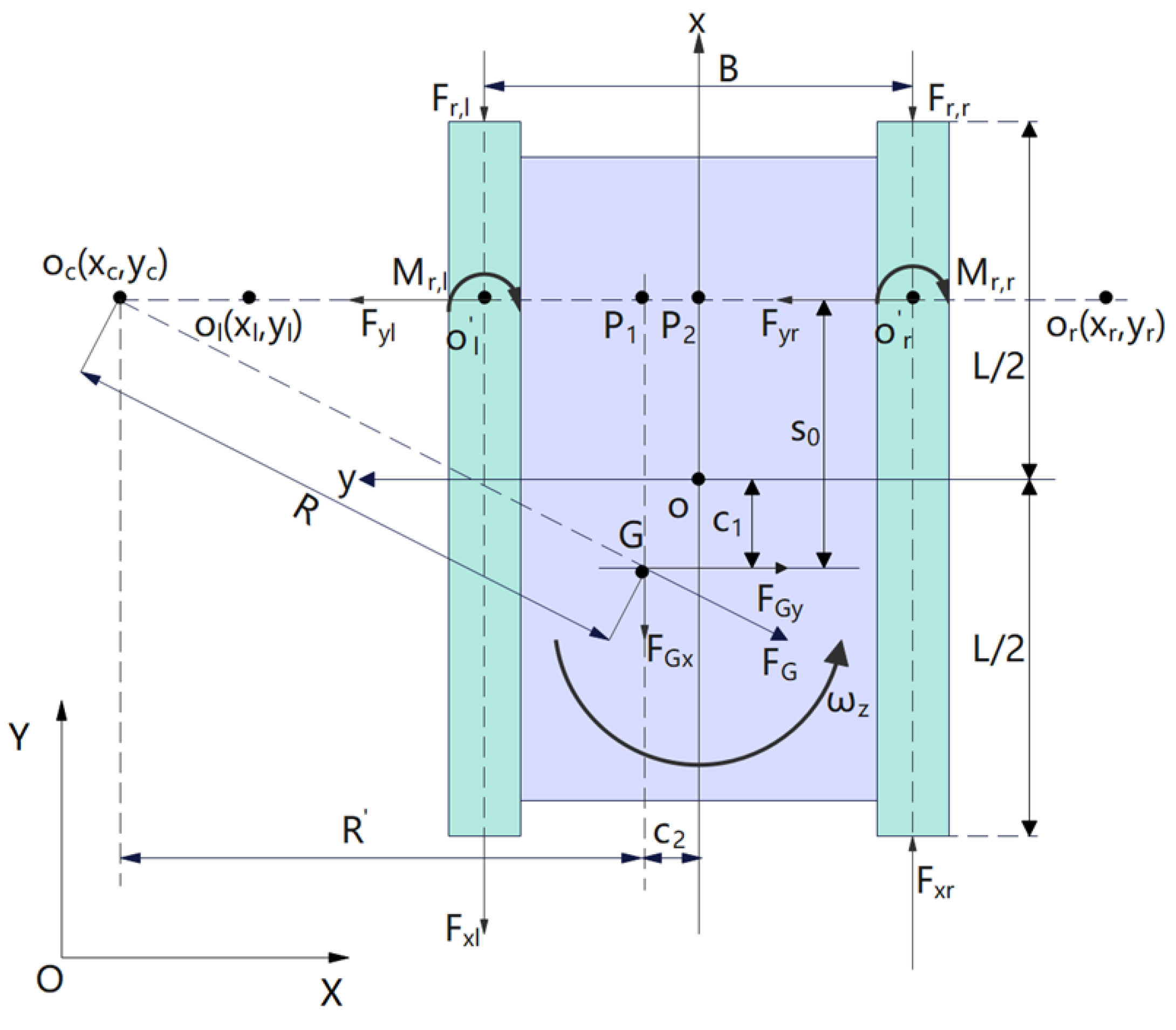
A simplified dynamic representation of the tracked vehicle is established based on the vehicle body-fixed frame. The force and moment definitions used in the dynamic analysis are illustrated in Figure 1. $G$ represents the vehicle’s center of mass, denoting the geometric center of the entire vehicle’s mass distribution; $P_1$ is the intersection point between the center of mass and the steering reference line; $P_2$ is the intersection point between the steering reference line and the longitudinal symmetry plane of the vehicle; $L$ denotes the length of the track’s ground contact section; $c_1$ and $c_2$ represent the positional deviations of the center of mass relative to the vehicle’s geometric center; $s_0$ indicates the longitudinal displacement of the steering reference line relative to the center of mass under centrifugal force; $R$ is the vehicle’s steady-state steering radius of curvature; $R^{\prime }$ denotes the vertical distance between the instantaneous steering center $O_{\mathrm{c}}$ of the vehicle body and the center of mass $G$; $F_{\mathrm{G}}$ represents the centrifugal inertial force during steering; The longitudinal and lateral components are denoted as $F_{\mathrm{G}\mathrm{x}}$ and $F_{\mathrm{G}\mathrm{y}}$ respectively; $F_{\mathrm{r},\mathrm{l}}$ and $F_{\mathrm{r},\mathrm{r}}$ represent the rolling resistance forces on the left and right track ground contact sections respectively; $F_{\mathrm{x}\mathrm{l}}$ and $F_{\mathrm{x}\mathrm{l}}$ denote the driving resultant force and braking resultant force on the left and right tracks, respectively; $F_{\mathrm{y}\mathrm{l}}$ and $F_{\mathrm{y}\mathrm{r}}$ denote the lateral components of tangential forces on the left and right tracks, respectively; $M_{\mathrm{r},\mathrm{l}}$ and $M_{\mathrm{r},\mathrm{r}}$ represent the steering resistance moments about the instantaneous rotation centers $O_{\mathrm{l}}^{\prime }$ and $O_{\mathrm{r}}^{\prime }$ of the left and right tracks around their respective ground segments. The track gauge (distance between the centers of the two tracks) is $B$.

With the above definitions, the dynamic equations of motion written in the body-fixed frame can be expressed as:

$$\begin{array}{c}\left\{\begin{array}{c}\delta m{\dot{v}}_{\mathrm{x}}=F_{\mathrm{x}\mathrm{r}}-F_{\mathrm{x}\mathrm{l}}-F_{\mathrm{r},\mathrm{l}}-F_{\mathrm{r},\mathrm{r}}-F_{\mathrm{G}\mathrm{x}}\\ m{\dot{v}}_{\mathrm{y}}=F_{\mathrm{y}\mathrm{l}}+F_{\mathrm{y}\mathrm{r}}-F_{\mathrm{G}\mathrm{y}}\\ {J\dot{\omega }}_z={\displaystyle \frac{B}{2}}\left(F_{\mathrm{x}\mathrm{l}}+F_{\mathrm{x}\mathrm{r}}+F_{\mathrm{r},\mathrm{l}}-F_{\mathrm{r},\mathrm{r}}\right)+F_{\mathrm{G}\mathrm{x}}{c}_2+F_{\mathrm{G}\mathrm{y}}{s}_0-\left(M_{\mathrm{r},\mathrm{l}}+M_{\mathrm{r},\mathrm{r}}\right)\end{array}\right.\end{array}$$

(1)

where $m$ is the vehicle mass, $\delta$ is the rotational mass conversion coefficient, $J$ is the yaw moment of inertia about the $z$-axis, $v_{\mathrm{x}}$ and $v_{\mathrm{y}}$ are the longitudinal and lateral velocities, and ${\omega }_z$ is the yaw rate.

For steady-state turning on flat terrain, solving the above equations yields the longitudinal forces on the left and right tracks:

$$\begin{array}{c}\left\{\begin{array}{c}{s}_0=c_1+{\displaystyle \frac{L{F}_{\mathrm{G}\mathrm{y}}}{2\mu mg}}\\ F_{\mathrm{x}\mathrm{l}}=-\left[F_{\mathrm{r},\mathrm{l}}+{\displaystyle \frac{1}{2}}{F}_{\mathrm{G}\mathrm{x}}+{\displaystyle \frac{1}{B}}\left(F_{\mathrm{G}\mathrm{x}}{c}_2+F_{\mathrm{G}\mathrm{y}}{s}_0-M_{\mathrm{r},\mathrm{l}}-M_{\mathrm{r},\mathrm{r}}\right)\right]\\ F_{\mathrm{x}\mathrm{r}}=F_{\mathrm{r},\mathrm{r}}+{\displaystyle \frac{1}{2}}{F}_{\mathrm{G}\mathrm{x}}-{\displaystyle \frac{1}{B}}\left(F_{\mathrm{G}\mathrm{x}}{c}_2+F_{\mathrm{G}\mathrm{y}}{s}_0-M_{\mathrm{r},\mathrm{l}}-M_{\mathrm{r},\mathrm{r}}\right)\end{array}\right.\end{array}$$

(2)

where $\mu$ is the turning resistance coefficient. In practice, $\mu$ is selected according to empirical data ($\mu =0.55{\mu }_{\mathrm{m}\mathrm{a}\mathrm{x}}$), and ${\mu }_{\mathrm{m}\mathrm{a}\mathrm{x}}$ denotes the maximum turning resistance coefficient. The steering resistance moments $M_{\mathrm{r},\mathrm{l}}$ and $M_{\mathrm{r},\mathrm{r}}$ can be computed from the lateral force components with respect to the vehicle mass center.

Instead of directly using the full dynamic model as the prediction model which would increase online computational burden, the derived longitudinal track forces are used to obtain physically meaningful actuator constraints (torque/power and acceleration bounds) for the predictive controller.

The choice of a kinematic model rather than a full dynamic model as the NMPC prediction model is justified by the following considerations. First, the full dynamic model involves highly nonlinear and coupled equations of motion, including track–terrain interaction forces, turning resistance moments, and load-dependent longitudinal forces, as described above. Incorporating such a model directly into the online NMPC optimization would substantially increase the computational complexity of the prediction and optimization steps, making real-time execution impractical on embedded agricultural control hardware with limited computational resources. Second, for trajectory tracking at the moderate operating speeds typical of orchard agricultural vehicles, the dominant motion characteristics are well captured by the kinematic relationships, and the dynamic effects are primarily manifested as time-varying slip rather than as significant inertial transients. These slip effects are explicitly addressed in the proposed framework through online parameter estimation as described in Section 2.2, rather than through direct dynamic modeling. Third, kinematic model-based NMPC has been widely validated for skid-steered and tracked vehicle trajectory tracking in the literature, demonstrating that accurate tracking performance can be achieved without requiring a full dynamic prediction model when appropriate slip compensation mechanisms are in place. The dynamic model developed in this section therefore serves a different but complementary role: it provides the physical basis for deriving actuator constraints—specifically the track force limits, torque requirements, and acceleration bounds given in Equations (23)–(25), which are enforced in the NMPC optimization to ensure that all computed control inputs remain physically realizable throughout the experiment.

2.1.2. Kinematic Model Based on the Instantaneous Center of Rotation

For real-time trajectory tracking control, a kinematic model is adopted as the prediction model of the NMPC controller. The tracked vehicle is modeled as a skid-steered system, where the motion of the vehicle can be described by the instantaneous center of rotation (ICR). The ICR-based modeling framework allows slip–skid effects to be implicitly captured through geometric relationships, making it suitable for tracked vehicle applications.

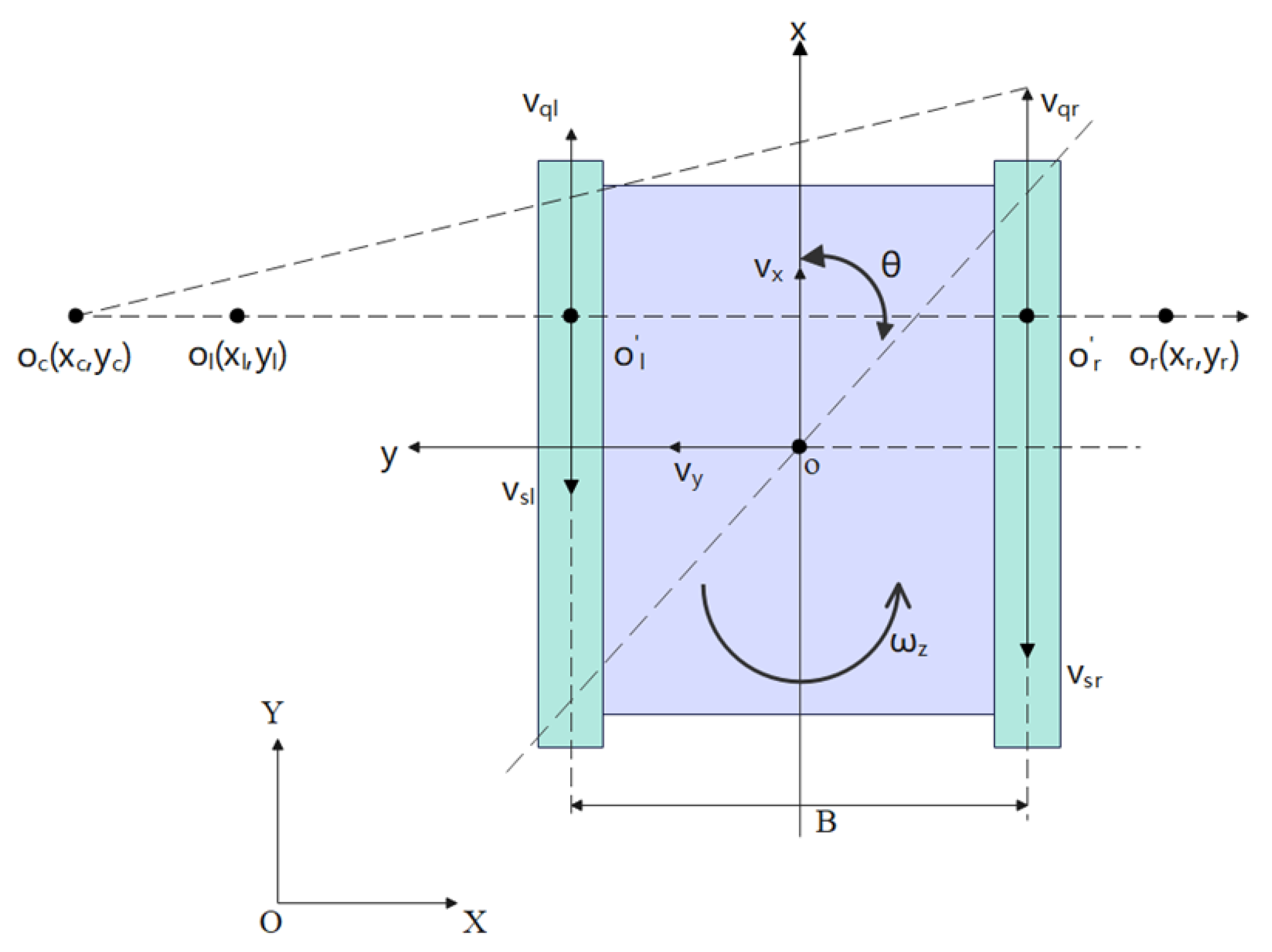
As shown in Figure 2, an inertial global coordinate frame $\left\{\mathrm{X}\mathrm{O}\mathrm{Y}\right\}$ is established, and the vehicle pose is uniquely determined by the global position $(\mathrm{x},\mathrm{y})$ and the heading angle $\theta$. The vehicle center of mass is assumed to coincide with the geometric center $o$. A body-fixed coordinate frame $\left\{\mathrm{x}\mathrm{o}\mathrm{y}\right\}$ is defined, and for simplicity in modeling, the center of mass is assumed to be initially aligned with the geometric center, which mean that the origin $o$ overlaps with the geometric center of the vehicle. The vehicle motion state is described by the longitudinal velocity $v_{\mathrm{x}}$ (along the $\mathrm{o}\mathrm{x}$-axis), the lateral velocity $v_{\mathrm{y}}$ (along the $\mathrm{o}\mathrm{y}$-axis), and the yaw rate ${\omega }_{\mathrm{z}}$ (about the $\mathrm{o}\mathrm{z}$-axis). The instantaneous center of rotation (ICR) of the vehicle body is denoted by $o_{\mathrm{c}}$, whose coordinates in the body-fixed frame are $(x_{\mathrm{c}},y_{\mathrm{c}})$, representing the instantaneous center about which the vehicle rotates. Let $o_{\mathrm{l}}$ and $o_{\mathrm{r}}$ denote the ICRs of the ground-contact segments of the left and right tracks, respectively, with coordinates $(x_{\mathrm{l}},y_{\mathrm{l}})$ and $(x_{\mathrm{r}},y_{\mathrm{r}})$ in the body-fixed frame. The points $o_{\mathrm{c}}$, $o_{\mathrm{l}}$ and $o_{\mathrm{r}}$ are collinear; this line is parallel to the lateral symmetry plane of the vehicle and is defined as the steering reference line, which passes through the vehicle-body ICR $o_{\mathrm{c}}$ and serves as a geometric reference for steering analysis. The intersections between the steering reference line and the perpendicular bisectors of the left and right track ground-contact segments define the ICRs of the ground-contact segments, denoted by $o_{\mathrm{l}}^{\prime }$ and $o_{\mathrm{r}}^{\prime }$ respectively. The velocities $v_{\mathrm{s}\mathrm{l}}$ and $v_{\mathrm{s}\mathrm{r}}$ denote the relative motion velocities of the left and right track ground-contact portions with respect to the vehicle body. These velocities arise from the track wrapping motion around the drive sprocket and the road wheels. Under pure straight-line motion without slip, there is no relative slip between the track ground-contact segment and the ground, and the magnitude of the wrapping speed equals the vehicle longitudinal speed $v_{\mathrm{x}}$. The velocities $v_{\mathrm{q}\mathrm{l}}$ and $v_{\mathrm{q}\mathrm{r}}$ denote the transport (kinematic) velocities of the vehicle body at points $o_{\mathrm{l}}^{\prime }$ and $o_{\mathrm{r}}^{\prime }$ respectively. When the vehicle undergoes pure rotation about the steering reference line, the points $o_{\mathrm{l}}^{\prime }$ and $o_{\mathrm{r}}^{\prime }$ lie on the rotation center line, and the corresponding transport velocities are zero. Here, $B$ denotes the center-to-center distance between the left and right tracks.

Under the ICR assumption, the vehicle motion can be expressed as a nonlinear kinematic model, where the control inputs are the left and right track velocities. This formulation avoids the assumption of pure rolling contact and allows the effects of track slip to be incorporated through effective ICR parameters. The shown kinematic equation can be described as:

$$\left[\begin{array}{c}\dot{x}\\ \dot{y}\\ \dot{\theta }\end{array}\right]=\left[\begin{array}{ccc}\mathrm{c}\mathrm{o}\mathrm{s}\theta & -\mathrm{s}\mathrm{i}\mathrm{n}\theta & 0\\ \mathrm{s}\mathrm{i}\mathrm{n}\theta & \mathrm{c}\mathrm{o}\mathrm{s}\theta & 0\\ 0& 0& 1\end{array}\right]\left[\begin{array}{c}{\displaystyle \frac{y_{\mathrm{l}}{v}_{\mathrm{s}\mathrm{r}}-y_{\mathrm{r}}{v}_{\mathrm{s}\mathrm{l}}}{y_{\mathrm{l}}-y_{\mathrm{r}}}}\\ {\displaystyle \frac{v_{\mathrm{s}\mathrm{l}}-v_{\mathrm{s}\mathrm{r}}}{y_{\mathrm{l}}-y_{\mathrm{r}}}}{x}_{\mathrm{c}}\\ -{\displaystyle \frac{v_{\mathrm{s}\mathrm{l}}-v_{\mathrm{s}\mathrm{r}}}{y_{\mathrm{l}}-y_{\mathrm{r}}}}\end{array}\right]=\mathit{R}\left(\theta \right)u$$

(3)

where $R\left(\theta \right)$ is the coefficient matrix related to the vehicle heading angle and instantaneous steering center, $u$ represents the control input, $u=[v_{\mathrm{s}\mathrm{l}},v_{\mathrm{s}\mathrm{r}}{]}^{\mathsf{{\rm T}}}$.

2.1.3. Kinematic Model Under Uneven Terrain Conditions

In orchard environments, uneven terrain induces vehicle roll and pitch motions, which alter load distribution and track–terrain contact conditions. These posture variations lead to coupling effects between translational and rotational motion, which cannot be captured by conventional planar kinematic models.

To account for these effects, vehicle roll angle and pitch angle are incorporated into the kinematic model. By applying a rotation transformation from the body-fixed frame to the global inertial frame, the vehicle velocities are projected onto the global coordinate system. As a result, the vehicle motion model explicitly reflects the influence of three-dimensional posture variations on trajectory evolution. The final improved kinematic model is:

$$\left[\begin{array}{c}\dot{x}\\ \dot{y}\\ \dot{\theta }\end{array}\right]=\left[\begin{array}{ccc}\mathrm{c}\mathrm{o}\mathrm{s}\theta \mathrm{c}\mathrm{o}\mathrm{s}\beta & \mathrm{c}\mathrm{o}\mathrm{s}\theta \mathrm{s}\mathrm{i}\mathrm{n}\beta \mathrm{s}\mathrm{i}\mathrm{n}\gamma -\mathrm{s}\mathrm{i}\mathrm{n}\theta \mathrm{c}\mathrm{o}\mathrm{s}\gamma & 0\\ \mathrm{s}\mathrm{i}\mathrm{n}\theta \mathrm{c}\mathrm{o}\mathrm{s}\beta & \mathrm{s}\mathrm{i}\mathrm{n}\theta \mathrm{s}\mathrm{i}\mathrm{n}\beta \mathrm{s}\mathrm{i}\mathrm{n}\gamma +\mathrm{c}\mathrm{o}\mathrm{s}\theta \mathrm{c}\mathrm{o}\mathrm{s}\gamma & 0\\ 0& 0& 1\end{array}\right]\left[\begin{array}{cc}-{\displaystyle \frac{y_{\mathrm{r}}}{y_l-y_r}}& {\displaystyle \frac{y_{\mathrm{l}}}{y_l-y_r}}\\ {\displaystyle \frac{x_{\mathrm{c}}}{y_{\mathrm{l}}-y_{\mathrm{r}}}}& -{\displaystyle \frac{x_{\mathrm{c}}}{y_{\mathrm{l}}-y_{\mathrm{r}}}}\\ -{\displaystyle \frac{1}{y_{\mathrm{l}}-y_{\mathrm{r}}}}& {\displaystyle \frac{1}{y_{\mathrm{l}}-y_{\mathrm{r}}}}\end{array}\right]\left[\begin{array}{c}{v}_{\mathrm{s}\mathrm{l}}\\ v_{\mathrm{s}\mathrm{r}}\end{array}\right]$$

(4)

where $\theta$ represents the heading angle of the tracked vehicle, $\beta$ represents the pitch angle, and $\gamma$ represents the roll angle. Within the rotation matrix on the right-hand side of the equation, the first column elements denote the projection components of the vehicle’s longitudinal velocity in the global coordinate system; the second column elements denote the projection components of the vehicle’s lateral velocity in the global coordinate system; and the third column elements denote the projection components of the rate of change in the heading angle.

The resulting nonlinear kinematic model provides a more accurate prediction of vehicle motion under uneven terrain conditions and serves as the prediction model for the NMPC controller.

2.2. Online Slip Parameter Estimation

Slip–skid effects are unavoidable for tracked agricultural vehicles operating on soft soil and uneven terrain, particularly in orchard environments. Track slip characteristics vary with terrain properties, vehicle load, and operating conditions, which leads to time-varying model parameters and degraded prediction accuracy if fixed parameters are assumed. To mitigate model mismatch and improve trajectory tracking performance, an online slip parameter estimation method is incorporated into the control framework.

2.2.1. Slip Mapping Model Based on Track Wrapping Velocities

In the ICR-based kinematic modeling framework, slip effects are reflected by the deviation of the instantaneous center of rotation from its ideal position. Under ideal conditions without slip, the instantaneous centers of rotation of the left and right tracks are located symmetrically at the centerlines of the tracks. However, under realistic operating conditions, slip causes these instantaneous centers to shift, resulting in discrepancies between predicted and actual vehicle motion.

To capture this behavior, slip parameters are introduced to describe the effective longitudinal positions of the instantaneous centers of rotation of the left and right tracks. These parameters implicitly represent the combined effects of track–terrain interaction, load distribution, and soil deformation, and are treated as unknown, time-varying quantities to be estimated online.

In the ICR-based kinematic model, the longitudinal coordinates of the instantaneous centers of rotation of the left and right track–ground contact segments, denoted by $y_{\mathrm{l}}$ and $y_{\mathrm{r}}$, characterize the slip–skid behavior during turning. In the ideal case (without slip), the ICRs of the two contact segments are located at the midpoints of the track contact patches, yielding $y_{\mathrm{l}}={\displaystyle \frac{B}{2}}$, $y_{\mathrm{r}}=-{\displaystyle \frac{B}{2}}$, $x_{\mathrm{c}}=0$, where $B$ is the track gauge (distance between the centers of the two tracks) and $x_{\mathrm{c}}$ is the longitudinal coordinate of the vehicle ICR in the body-fixed frame.

The slip parameters during turning are strongly correlated with the left and right track wrapping velocities $v_{\mathrm{s}\mathrm{l}}$ and $v_{\mathrm{s}\mathrm{r}}$. Therefore, the slip parameters are modeled by the following nonlinear mapping:

$$\begin{array}{c}\left\{\begin{array}{c}{y}_{\mathrm{l}}={\displaystyle \frac{B}{2}}+k_1\left|\left(v_{\mathrm{s}\mathrm{l}}-v_{\mathrm{s}\mathrm{r}}\right)\left(v_{\mathrm{s}\mathrm{l}}+v_{\mathrm{s}\mathrm{r}}\right)\right|+k_2\\ y_{\mathrm{r}}=-{\displaystyle \frac{B}{2}}+k_3\left|\left(v_{\mathrm{s}\mathrm{l}}-v_{\mathrm{s}\mathrm{r}}\right)\left(v_{\mathrm{s}\mathrm{l}}+v_{\mathrm{s}\mathrm{r}}\right)\right|+k_4\\ x_{\mathrm{c}}=k_5\left|\left(v_{\mathrm{s}\mathrm{l}}-v_{\mathrm{s}\mathrm{r}}\right)\left(v_{\mathrm{s}\mathrm{l}}+v_{\mathrm{s}\mathrm{r}}\right)\right|+k_6\left|{\displaystyle \frac{v_{\mathrm{s}\mathrm{l}}-v_{\mathrm{s}\mathrm{r}}}{v_{\mathrm{s}\mathrm{l}}+v_{\mathrm{s}\mathrm{r}}}}\right|\end{array}\right.\end{array}$$

(5)

where k₁∼k₆ are unknown coefficients describing the nonlinear coupling between track velocities and slip-related ICR parameters. In this work, the Levenberg–Marquardt (L–M) algorithm is used to estimate k₁∼k₆ online, and the resulting $y_{\mathrm{l}},y_{\mathrm{r}}$, $x_{\mathrm{c}}$ are obtained by substituting the estimated coefficients into (5).

2.2.2. Least-Squares Formulation

To minimize the mismatch between the predicted and measured vehicle pose, the online estimation is formulated as a nonlinear least-squares problem. Let

$$m={[k_1,k_2,k_3,k_4,k_5,k_6]}^{\mathsf{{\rm T}}}$$

be the parameter vector to be estimated. Suppose $n$ pose samples are collected within a sliding window. For the $i$-th sample, define the pose residual as

$$\begin{array}{c}{p}_i\left(m\right)=p_{\mathrm{m},\mathrm{i}}\left(m\right)-p_{\mathrm{e},\mathrm{i}}\left(m\right)={\left[x_{\mathrm{m},\mathrm{i}}\left(m\right),y_{\mathrm{m},\mathrm{i}}\left(m\right),{\theta }_{\mathrm{m},\mathrm{i}}\left(m\right)\right]}^{\mathsf{{\rm T}}}-{\left[x_{\mathrm{e},\mathrm{i}}\left(m\right),y_{\mathrm{e},\mathrm{i}}\left(m\right),{\theta }_{\mathrm{e},\mathrm{i}}\left(m\right)\right]}^{\mathsf{{\rm T}}}\end{array}$$

(6)

where $p_{\mathrm{m},\mathrm{i}}\left(m\right)$ is the measured pose and $p_{\mathrm{e},\mathrm{i}}\left(m\right)$ is the predicted pose obtained from the kinematic model using the slip parameters computed from (5) under the current time $m$. The stacked residual vector is

$$\begin{array}{c}P\left(m\right)={\left[p_1^{\mathsf{{\rm T}}}\left(m\right),p_2^{\mathsf{{\rm T}}}\left(m\right),\dots ,p_{\mathrm{n}}^{\mathsf{{\rm T}}}\left(m\right)\right]}^{\mathsf{{\rm T}}}\end{array}$$

(7)

The objective function is defined as

$$\begin{array}{c}J\left(m\right)={\displaystyle \frac{1}{2}}{\displaystyle \sum _{\mathrm{i}=1}^n}{‖p_{\mathrm{i}}\left(m\right)‖}^2={\displaystyle \frac{1}{2}}{P}^{\mathsf{{\rm T}}}\left(m\right)P(m)\end{array}$$

(8)

The optimal parameter estimate is obtained by minimizing $J\left(m\right)$ iteratively.

2.2.3. Levenberg–Marquardt Update and Jacobian

The L–M algorithm was selected over alternative online estimation methods, such as the Extended Kalman Filter (EKF) and sliding-mode observers, for the following reasons. First, the relationship between slip parameters and track wrapping velocities defined in Equation (5) is inherently nonlinear. EKF-based approaches require linearization of the nonlinear system at each time step via Jacobian computation, which can introduce non-negligible linearization errors when the slip dynamics exhibit strong nonlinearity during sharp turning maneuvers on soft soil. In contrast, the L–M algorithm directly minimizes the nonlinear least-squares pose residual without requiring explicit linearization, making it better suited to the strongly nonlinear slip mapping in this application. Second, the L–M algorithm adaptively adjusts the damping factor $\lambda$ during iterations: a larger $\lambda$ biases the update toward gradient descent to ensure stability in early iterations, while a smaller $\lambda$ approaches the Gauss–Newton step for faster convergence near the solution. This adaptive mechanism provides robust convergence under the varying terrain and load conditions encountered in orchard environments, without the need for gain scheduling that would otherwise be required by sliding-mode or adaptive observer approaches. Third, compared with state observer-based methods that require a precisely defined state-space model structure and formal stability proofs for each operating condition, the L–M algorithm is straightforward to implement on embedded agricultural control hardware and does not require prior structural knowledge of the slip dynamics. These properties collectively make the L–M algorithm a pragmatic and effective choice for real-time slip parameter estimation in unstructured orchard environments.

Because the prediction model is nonlinear, directly optimizing $J\left(m\right)$ may lead to poor convergence. Thus, the residual vector is linearized at the current estimate $m$ via a first-order Taylor expansion:

$$\begin{array}{c}\mathit{P}\left(m+h\right)\approx \mathit{P}\left(m\right)+\mathit{H}\left(m\right)h\end{array}$$

(9)

where $h$ is the parameter increment and $H\left(m\right)$ is the Jacobian matrix.

To improve robustness when $H^{\mathsf{{\rm T}}}H$ is ill-conditioned, a damping factor $\lambda$ is introduced. The L–M increment is computed from the normal equation:

$$\begin{array}{c}\left[{\mathit{H}}^{\mathsf{{\rm T}}}\left(m\right)\mathit{H}\left(m\right)+\lambda \mathit{I}\right]h={\mathit{H}}^{\mathsf{{\rm T}}}\left(m\right)P\left(m\right)\end{array}$$

(10)

where $I$ is the identity matrix. During iterations, $\lambda$ is adjusted dynamically: a larger $\lambda$ makes the update closer to gradient descent for stability, while a smaller $\lambda$ approaches the Gauss–Newton step for faster convergence.

The Jacobian $H\left(m\right)$ is defined as the sensitivity of the pose residual with respect to the parameter vector $m$. For the $j$-th iteration, it can be written as

$$\begin{array}{c}{H}^{\left(j\right)}\left(m\right)={\displaystyle \frac{\partial P}{\partial m}}=\left(\begin{array}{c}{\displaystyle \frac{\partial \left(p_{\mathrm{m},\mathrm{x}}-p_{\mathrm{e},\mathrm{x}}\right)}{\partial k_1~k_6}}\\ {\displaystyle \frac{\partial \left(p_{\mathrm{m},\mathrm{y}}-p_{\mathrm{e},\mathrm{y}}\right)}{\partial k_1~k_6}}\\ {\displaystyle \frac{\partial \left(p_{\mathrm{m},\mathsf{\theta }}-p_{\mathrm{e},\mathsf{\theta }}\right)}{\partial k_1~k_6}}\end{array}\right)\end{array}$$

(11)

where $p_{\mathrm{e},\mathrm{x}},p_{\mathrm{e},\mathrm{y}},p_{\mathrm{e},\mathsf{\theta }}$ are the predicted pose components computed using the current parameter estimate.

In the proposed implementation, the following specific settings are adopted for the online estimation procedure. The pose measurements used for residual computation are provided by the onboard GNSS/IMU system at a sampling frequency of 10 Hz. The parameter vector m is initialized to zero at the start of operation ($m_0=0$), corresponding to the assumption of an ideal slip-free initial state; the damping factor λ is initialized to 0.1. Three termination conditions are applied within each estimation cycle: (1) $‖g‖\le {\epsilon }_1$ with $g=-H{\left(m\right)}^{T}P\left(m\right)$ and ${\epsilon }_1={10}^{-8}$, indicating convergence to a local minimum; (2) $k\ge k\_max$ with $k_{\mathrm{m}\mathrm{a}\mathrm{x}}=50$, limiting the maximum number of iterations; and (3) $‖h‖\le {\epsilon }_2(‖m‖+{\epsilon }_2)$ with ${\epsilon }_2={10}^{-6}$, indicating a sufficiently small update step. During iterations, $\lambda$ is reduced by a factor of 0.1 when $J\left(m\right)$ decreases $(\mathsf{\Delta }J\left(m\right)=J\left(m\right)-J(\mathit{\text{m\_new}})>0)$, and increased by a factor of 10 otherwise. At each control step, the updated slip parameters $y_{\mathrm{l}}$, $y_{\mathrm{r}}$, and $x_{\mathrm{c}}$ obtained from the current estimate of m are immediately substituted into the NMPC prediction model to update the kinematic state predictions for the current optimization cycle.

2.3. NMPC Formulation for Trajectory Tracking

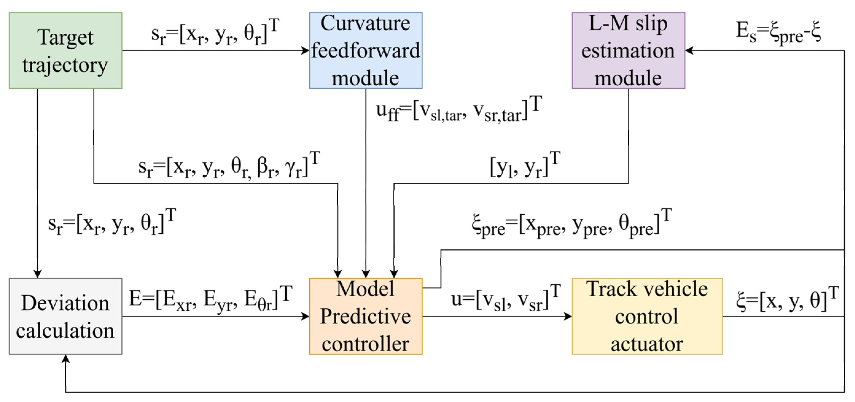
As illustrated in Figure 3, the proposed control framework consists of four interconnected modules. The target trajectory provides the reference pose $s_{\mathrm{r}}={[x_{\mathrm{r}},y_{\mathrm{r}},{\theta }_{\mathrm{r}}]}^T$ and path curvature $k$ to the Curvature Feedforward Module, which computes the feedforward track velocity reference $u_{\mathrm{f}\mathrm{f}}={[v_{\mathrm{s}\mathrm{l},\mathrm{t}\mathrm{a}\mathrm{r}},v_{\mathrm{s}\mathrm{r},\mathrm{t}\mathrm{a}\mathrm{r}}]}^T$ based on the desired forward speed and path geometry. Simultaneously, the onboard GNSS/IMU system provides the actual vehicle pose $\xi ={[x,y,\theta ]}^T$, which is fed into both the Deviation Calculation Module and the L–M Algorithm Parameter Estimation Module. The L–M estimator updates the slip parameters $y_{\mathrm{l}}$ and $y_{\mathrm{r}}$ online by minimizing the positioning deviation $E_{\mathrm{s}}={\xi }_{\mathrm{p}\mathrm{r}\mathrm{e}}-\xi$ between the predicted state ${\xi }_{\mathrm{p}\mathrm{r}\mathrm{e}}={[x_{\mathrm{p}\mathrm{r}\mathrm{e}},y_{\mathrm{p}\mathrm{r}\mathrm{e}},{\theta }_{\mathrm{p}\mathrm{r}\mathrm{e}}]}^T$ and the measured pose. The updated slip parameters are incorporated into the prediction model of the Model Predictive Controller, which receives the tracking error $E=S_{\mathrm{r}}-S={[E_{\mathrm{x}\mathrm{r}},E_{\mathrm{y}\mathrm{r}},E_{\mathsf{\theta }\mathrm{r}}]}^T$ and solves the constrained optimization problem to generate the optimal control input $u={[s_{\mathrm{l}},s_{\mathrm{r}}]}^T$. The computed commands are then applied to the Track Vehicle Control Actuator to drive the vehicle along the reference trajectory.

2.3.1. Discrete-Time Prediction Model

The vehicle kinematic model is inherently nonlinear and can be expressed in a continuous-time state-space form. For implementation in the NMPC framework, the continuous-time model is discretized using a forward Euler method with a fixed sampling period $T_{\mathrm{s}}$.

The discrete-time nonlinear prediction model can be written as:

$$\begin{array}{c}\dot{\xi }=f\left(\mathit{\xi },\mathit{u}\right)\end{array}$$

(12)

where $\mathsf{\xi }$ denotes the vehicle state vector, $\xi ={\left[x,y,\theta \right]}^{\mathsf{{\rm T}}}$, $u$ is the control input, $\mathrm{u}={{[v}_{\mathrm{s}\mathrm{l}},v_{\mathrm{s}\mathrm{r}}]}^{\mathsf{{\rm T}}}$. By applying the forward Euler method to discretize the system, the discrete predictive model for NMPC is obtained as:

$$\begin{array}{c}\mathit{\xi }\left(k+1\right)=\mathsf{\xi }\left(k\right)+f\left(\mathsf{\xi }\left(k\right),\mathit{u}\left(k\right)\right)·T_{\mathrm{s}}\end{array}$$

(13)

where k denotes the kth time step, and $T_{\mathrm{s}}$ represents the discrete time step size.

2.3.2. Objective Function

To improve tracking performance in high-curvature segments and to reduce the computational burden of online optimization, a curvature-feedforward term is introduced to provide a physically meaningful reference for the control inputs. Instead of directly applying the feedforward command to the actuators, it is embedded into the NMPC objective as a reference input, such that the optimizer searches for an optimal solution in the neighborhood of the feedforward command while satisfying constraints and correcting tracking errors.

(1)

Curvature computation and feedforward reference generation

Given the reference trajectory $P_{\mathrm{r}}\left(s\right)=\left[x_{\mathrm{r}}\right(s),\hspace{0.17em}{y}_{\mathrm{r}}(s){]}^{\mathrm{T}}$, the path curvature $k\left(s\right)$ is computed based on the first- and second-order derivatives of the reference trajectory. In implementation, the derivatives are obtained using a central difference scheme. The curvature is calculated as:

$$\begin{array}{c}k\left(s\right)={\displaystyle \frac{x_{\mathrm{r}}^{\prime }\left(s\right)y_{\mathrm{r}}^{″}\left(s\right)-y_{\mathrm{r}}^{\prime }\left(s\right)x_{\mathrm{r}}^{″}\left(s\right)}{({x_{\mathrm{r}}^{\prime }\left(s\right)}^2+y_{\mathrm{r}}^{\prime }{\left(s\right)}^2{)}^{3/2}+\delta }}\end{array}$$

(14)

where ${(·)}^{\prime }$ and ${(·)}^{″}$ denote the first- and second-order derivatives with respect to the path parameter $s$, and $\delta >0$ is a small constant to avoid numerical singularity.

For a desired forward speed $v_{\mathrm{d}}$, the feedforward yaw rate is determined by the curvature:

$$\begin{array}{c}{\omega }_{\mathrm{f}\mathrm{f}}\left(s\right)=v_{\mathrm{d}}k\left(s\right)\end{array}$$

(15)

Using the differential-drive relationship for a tracked vehicle, the feedforward track velocities are generated as:

$$\begin{array}{c}{v}_{\mathrm{l},\mathrm{f}\mathrm{f}}\left(s\right)=v_{\mathrm{d}}-{\displaystyle \frac{B}{2}}{\omega }_{\mathrm{f}\mathrm{f}}\left(s\right)\end{array}$$

(16)

$$\begin{array}{c}{v}_{\mathrm{r},\mathrm{f}\mathrm{f}}\left(s\right)=v_{\mathrm{d}}+{\displaystyle \frac{B}{2}}{\omega }_{\mathrm{f}\mathrm{f}}\left(s\right)\end{array}$$

(17)

where $B$ is the center-to-center distance between the left and right tracks. The feedforward input vector is thus defined as:

$$\begin{array}{c}{u}_{\mathrm{f}\mathrm{f}}\left(s\right)=\left[\begin{array}{c}{v}_{\mathrm{l},\mathrm{f}\mathrm{f}}\left(s\right)\\ v_{\mathrm{r},\mathrm{f}\mathrm{f}}\left(s\right)\end{array}\right]\end{array}$$

(18)

In each control cycle, $u_{\mathrm{f}\mathrm{f}}$ is computed along the prediction horizon according to the reference trajectory and used as a reference input in the NMPC optimization.

(2)

NMPC objective function

Let the system state be ${\xi }_{\mathrm{k}}=[x_{\mathrm{k}},\hspace{0.17em}{y}_{\mathrm{k}},\hspace{0.17em}{\mathsf{\theta }}_{\mathrm{k}}{]}^{\mathrm{T}}$ and the control input be $u_{\mathrm{k}}=[v_{\mathrm{l},\mathrm{k}},\hspace{0.17em}{v}_{\mathrm{r},\mathrm{k}}{]}^{\mathrm{T}}$.

Denote the reference state at step $k+i$ by ${\xi }_{\mathrm{k}+\mathrm{i}}^{\mathrm{r}}=[x_{\mathrm{k}+\mathrm{i}}^{\mathrm{r}},\hspace{0.17em}{y}_{\mathrm{k}+\mathrm{i}}^{\mathrm{r}},\hspace{0.17em}{\theta }_{\mathrm{k}+\mathrm{i}}^{\mathrm{r}}{]}^{\mathrm{T}}$. The tracking error is defined as:

$$\begin{array}{c}{e}_{\mathrm{k}+\mathrm{i}}={\xi }_{\mathrm{k}+\mathrm{i}}-{\xi }_{\mathrm{k}+\mathrm{i}}^{\mathrm{r}}\end{array}$$

(19)

The NMPC objective over the prediction horizon $N_{\mathrm{p}}$ and control horizon $N_{\mathrm{c}}$ is formulated as:

$$\begin{array}{c}J={\displaystyle \sum _{i=1}^{N_{\mathrm{p}}}}{‖e_{\mathrm{k}+\mathrm{i}}‖}_{\mathit{Q}}^2+{\displaystyle \sum _{i=0}^{N_{\mathrm{c}}-1}}{‖u_{\mathrm{k}+\mathrm{i}}-u_{\mathrm{f}\mathrm{f},\mathrm{k}+\mathrm{i}}‖}_{\mathit{R}}^2+{\displaystyle \sum _{i=0}^{N_{\mathrm{c}}-1}}{‖\Delta u_{\mathrm{k}+\mathrm{i}}‖}_{\mathit{S}}^2+\rho {\epsilon }^2\end{array}$$

(20)

where $Q$, $R$ and $S$ are weighting matrices, $\mathsf{\Delta }{u}_{\mathrm{k}+\mathrm{i}}=u_{\mathrm{k}+\mathrm{i}}-u_{\mathrm{k}+\mathrm{i}-1}$ is the control increment, $\epsilon$ is a slack variable introduced for soft constraints, and $\rho >0$ is its penalty coefficient. Note that Q, R, and S are three distinct weighting matrices: Q penalizes the state tracking error, R penalizes deviation from the curvature feedforward reference $u_{\mathrm{f}\mathrm{f}}$, and S penalizes the control increment. These matrices are independently tuned to balance tracking accuracy, feedforward consistency, and control smoothness.

The objective consists of four terms:

(1)

The state tracking error term, which enforces accurate trajectory tracking in position and heading;

(2)

The curvature-feedforward consistency term, which penalizes deviations from the feedforward reference $u_{\mathrm{f}\mathrm{f}}$ and effectively guides the optimizer toward feasible turning commands in curved segments;

(3)

The control increment term, which suppresses excessive input variations and improves smoothness of track speed commands;

(4)

The slack penalty term, which guarantees feasibility when strict satisfaction of all constraints is not possible due to disturbances or modeling mismatch.

Introducing $u_{\mathrm{f}\mathrm{f}}$ as a reference input provides a good initial direction for turning maneuvers, thereby improving transient response in high-curvature segments and potentially reducing the number of iterations required by the online solver, while the feedback optimization still compensates for disturbances and slip-induced errors.

2.3.3. Constraints

Constraints in model predictive control can be explicitly categorized into two types: equality constraints and inequality constraints. In trajectory tracking control, equality constraints correspond to the vehicle’s kinematic model, describing the dynamic relationship between the current state and the future state. Inequality constraints, based on the physical limits of the vehicle’s actuators and control stability requirements, impose boundary restrictions on control inputs and their rates of change. This prevents actuator damage or system instability caused by excessive control actions or abrupt fluctuations. Therefore, it is essential to properly configure inequality constraints, which primarily include two types. The first is control input amplitude constraint:

$$\begin{array}{c}\left\{\begin{array}{c}{v}_{\mathrm{s}\mathrm{l},\mathrm{m}\mathrm{i}\mathrm{n}}\le v_{\mathrm{s}\mathrm{l}}\left(k\right)\le v_{\mathrm{s}\mathrm{l},\mathrm{m}\mathrm{a}\mathrm{x}}\\ v_{\mathrm{s}\mathrm{r},\mathrm{m}\mathrm{i}\mathrm{n}}\le v_{\mathrm{s}\mathrm{r}}\left(k\right)\le v_{\mathrm{s}\mathrm{r},\mathrm{m}\mathrm{a}\mathrm{x}}\end{array}\right.\end{array}$$

(21)

where $v_{\mathrm{s}\mathrm{l},\mathrm{m}\mathrm{i}\mathrm{n}}$ and $v_{\mathrm{s}\mathrm{r},\mathrm{m}\mathrm{i}\mathrm{n}}$ represent the lower limits of left and right track speeds, respectively; $v_{\mathrm{s}\mathrm{l},\mathrm{m}\mathrm{a}\mathrm{x}}$ and $v_{\mathrm{s}\mathrm{r},\mathrm{m}\mathrm{a}\mathrm{x}}$ represent the upper limits of left and right track speeds, respectively. These constraints ensure that track wheel speeds remain within the controllable output range of the actuators, preventing motor overload.

Incremental constraints on control variables are equally important:

$$\begin{array}{c}\left\{\begin{array}{c}\left|\mathsf{\Delta }{v}_{\mathrm{s}\mathrm{l}}\left(k\right)\right|=\left|v_{\mathrm{s}\mathrm{l}}\left(k\right)-v_{\mathrm{s}\mathrm{l}}\left(k-1\right)\right|\le \Delta v_{\mathrm{s}\mathrm{l},\mathrm{m}\mathrm{a}\mathrm{x}}\\ \left|\mathsf{\Delta }{v}_{\mathrm{s}\mathrm{r}}\left(k\right)\right|=\left|v_{\mathrm{s}\mathrm{r}}\left(k\right)-v_{\mathrm{s}\mathrm{r}}\left(k-1\right)\right|\le \Delta v_{\mathrm{s}\mathrm{r},\mathrm{m}\mathrm{a}\mathrm{x}}\end{array}\right.\end{array}$$

(22)

where $\mathsf{\Delta }{v}_{\mathrm{s}\mathrm{l},\mathrm{m}\mathrm{a}\mathrm{x}}$ and $\mathsf{\Delta }{v}_{\mathrm{s}\mathrm{r},\mathrm{m}\mathrm{a}\mathrm{x}}$ represent the upper limits for the rate of change in speed in the left and right track wheels, respectively. These constraints prevent abrupt changes in wheel speed, protect the transmission system, and minimize slippage as much as possible.

For the amplitude constraints and incremental constraints of the control variable in the above equation, these are typically directly determined by the drive motor. The drive motor exhibits operational characteristics of constant torque in the low-speed range and constant power in the high-speed range. By integrating these characteristics with the tracked vehicle dynamics model, the estimated values for braking force and driving force requirements, $F_{\mathrm{x}\mathrm{l}}$ and $F_{\mathrm{x}\mathrm{r}}$, can be derived from Equation (2). This further enables the estimation of the vehicle’s torque requirement during operation:

$$\begin{array}{c}\left\{\begin{array}{c}{T}_{\mathrm{x}\mathrm{l}}={\displaystyle \frac{F_{\mathrm{x}\mathrm{l}}r}{{\eta }_{\mathrm{e}}{i}_{\mathrm{o}}}}\\ T_{\mathrm{x}\mathrm{r}}={\displaystyle \frac{F_{\mathrm{x}\mathrm{r}}r}{{\eta }_{\mathrm{e}}{i}_{\mathrm{o}}}}\end{array}\right.\end{array}$$

(23)

where $T_{\mathrm{x}\mathrm{l}}$ and $T_{\mathrm{x}\mathrm{r}}$ represent the torque requirements for the left and right tracks during turning, respectively; $r$ denotes the radius of the track vehicle’s drive wheel; ${\eta }_{\mathrm{e}}$ indicates the overall transmission efficiency; and $i_{\mathrm{o}}$ signifies the overall transmission ratio.

The speed of a single track on a tracked vehicle is governed by the following inequality:

$$\begin{array}{c}\left|v_{\mathrm{s}}\right|\le {\displaystyle \frac{9550\pi r{P}_{\mathrm{m}\mathrm{a}\mathrm{x}}}{30k_{\mathrm{p}}\left|T_{\mathrm{x}}\right|}}\end{array}$$

(24)

where $v_{\mathrm{s}}$ denotes the speed of a single track; $P_{\mathrm{m}\mathrm{a}\mathrm{x}}$ represents the maximum motor power; $k_{\mathrm{p}}$ is the protection coefficient; $T_{\mathrm{x}}$ is the single-side torque requirement value obtained from Equation (23). This inequality yields the limiting value of the control variable in Equation (21).

Additionally, the acceleration of tracked vehicles should be subject to the following inequality constraints:

$$\begin{array}{c}\left|a\right|\le {\displaystyle \frac{\phi g-\left|F_{\mathrm{x}\mathrm{l}}\right|-\left|F_{\mathrm{x}\mathrm{r}}\right|}{m}}\end{array}$$

(25)

where $a$ represents vehicle acceleration; $\phi$ denotes the ground adhesion coefficient; $g$ is the gravitational acceleration. This equation yields the limiting value for the increment of the control variable in Equation (22).

These constraints ensure that the computed control inputs are physically realizable and suitable for real-world agricultural operations.

At each control cycle, the NMPC optimization problem is solved using the current vehicle state as the initial condition. Only the first control input in the optimal control sequence is applied to the vehicle, and the optimization is repeated at the next time step using updated state information, which enables the controller to adapt to disturbances, modeling uncertainties, and time-varying terrain conditions.

2.4. Experimental Platform and Test Environment

2.4.1. Tracked Agricultural Vehicle Platform

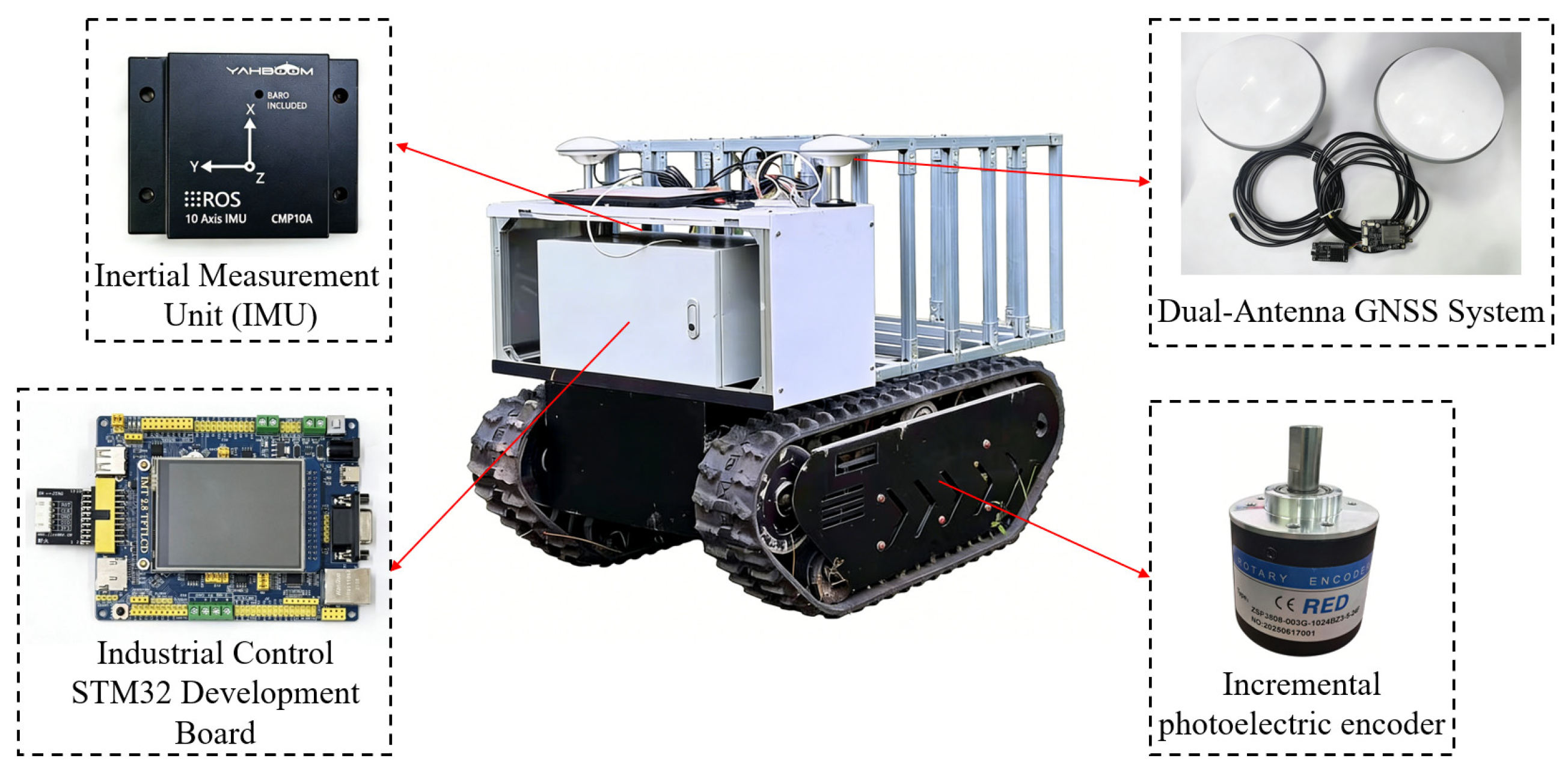
Field experiments were conducted using a self-developed tracked agricultural vehicle platform, as shown in Figure 4. The vehicle adopts a differential drive configuration with independently driven left and right tracks, which enables steering through track speed difference. This configuration is widely used in orchard and hilly agricultural environments due to its strong traction capability and adaptability to uneven terrain.

The experimental platform is equipped with the following sensing and actuation components. Each track is independently driven by a DC servo motor (rated power 1600 W, rated voltage 48 V, rated torque 60 N·m) controlled by a KYDAS48150-2E motor driver (Jinan Keya Electron Science and Technology Co., Ltd., Jinan, China) operating in closed-loop velocity control mode. The detailed electrical and mechanical parameters of the motor (model KY130ACS0430-30B, Jinan Keya Electron Science and Technology Co., Ltd., Jinan, China) are as follows: wire resistance R = 0.02 Ω, line inductance L = 0.03 mH, moment of inertia J = 48 × 10⁻⁴ kg·m², torque constant Kt = 0.25 N·m/A, and back-EMF constant Ke = 23.5 V/krpm. Note that the rated power and torque values represent the output specifications at the drive wheel shaft after the gearbox transmission, whereas the above electrical parameters are those of the motor itself. The onboard control unit communicates with the motor drivers via RS232 serial interface, with a software-level timestamp compensation mechanism limiting the communication-induced delay to within 5 ms, which is negligible relative to the 100 ms control cycle. The actuator constraints applied in the NMPC—specifically the track speed limit $v_{\mathrm{s},\mathrm{m}\mathrm{a}\mathrm{x}}=\pm 0.6 \mathrm{m}/\mathrm{s}$ and the speed increment limit $\mathsf{\Delta }{v}_{\mathrm{s},\mathrm{m}\mathrm{a}\mathrm{x}}=0.1 \mathrm{m}/\mathrm{s}$—were derived from the motor rated torque, maximum power rating, drive wheel radius (r = 110 mm), and ground adhesion coefficient ($\varphi =0.55$) measured at the test site, following the dynamic constraint derivation procedure described in Equations (23)–(25).

High-accuracy position and heading information is provided by a Unicore Communications NebulasIV series dual-antenna GNSS system (Unicore Communications, Inc., Beijing, China), achieving centimeter-level RTK positioning accuracy with a data update rate of 10 Hz. This provides reliable heading estimation even at low vehicle speeds, which is particularly important for trajectory tracking experiments. Vehicle attitude information—including the roll and pitch angles required by the improved three-dimensional kinematic model—is provided by an onboard IMU with a default output rate of 10 Hz, a static roll/pitch accuracy of 0.1°, and a dynamic roll/pitch accuracy of 0.5°. Track wrapping velocities are measured by incremental photoelectric encoders (1024 PPR, maximum response frequency 100 kHz) mounted on the drive sprockets. All sensor data are fused and processed by an onboard industrial control STM32 development board (STMicroelectronics, Geneva, Switzerland), which executes the proposed NMPC algorithm in real time and generates control commands for the track drive motors.

The vehicle state information, including position, velocity, and attitude, is updated at a fixed sampling frequency of 10 Hz and transmitted to the NMPC controller for trajectory prediction and optimization. The control commands computed by the controller are directly applied to the track motors, enabling closed-loop trajectory tracking under real agricultural operating conditions.

The key specifications of the vehicle and the sensors and actuators used in the experimental platform are summarized in

Table 1. Track Vehicle Specifications.

Category	Parameter	Value	Unit
Vehicle	Overall Dimensions	1300 × 820 × 530	mm
	Weight	220	kg
	Track Center Distance B	680	mm
	Track Ground Contact Length	950	mm
	Track Width b	150	mm
	Center of Gravity Height h	250	mm
Drive System	Drive Wheel Radius	110	mm
	Motor Type	DC Servo Motor	-
	Maximum Motor Power P	1600	W
	Rated Motor Torque	60	N·m
	Motor Driver Model	KYDAS48150-2E	-
	Control Mode	Closed-loop velocity	-
	Wire Resistance	0.02	Ω
	Line Inductance	0.03	mH
	Moment of Inertia	48 × 10−4	kg·m2
	Torque Constant	0.25	N·m/A
	Back-EMF Constant	23.5	V/krpm
GNSS	Positioning Accuracy	RTK cm-level	-
	Update Rate	10	Hz-
	Heading Mode	Dual-antenna	-
IMU	Output Rate	10	Hz
	Static Roll/Pitch Accuracy	0.1	°
	Dynamic Roll/Pitch Accuracy	0.5	°
Encoder	Resolution	1024	PPR
Controller	Control Cycle	100	ms
	Communication Interface	RS232	-
	Communication Delay	≤5	ms

.

2.4.2. Test Site Description

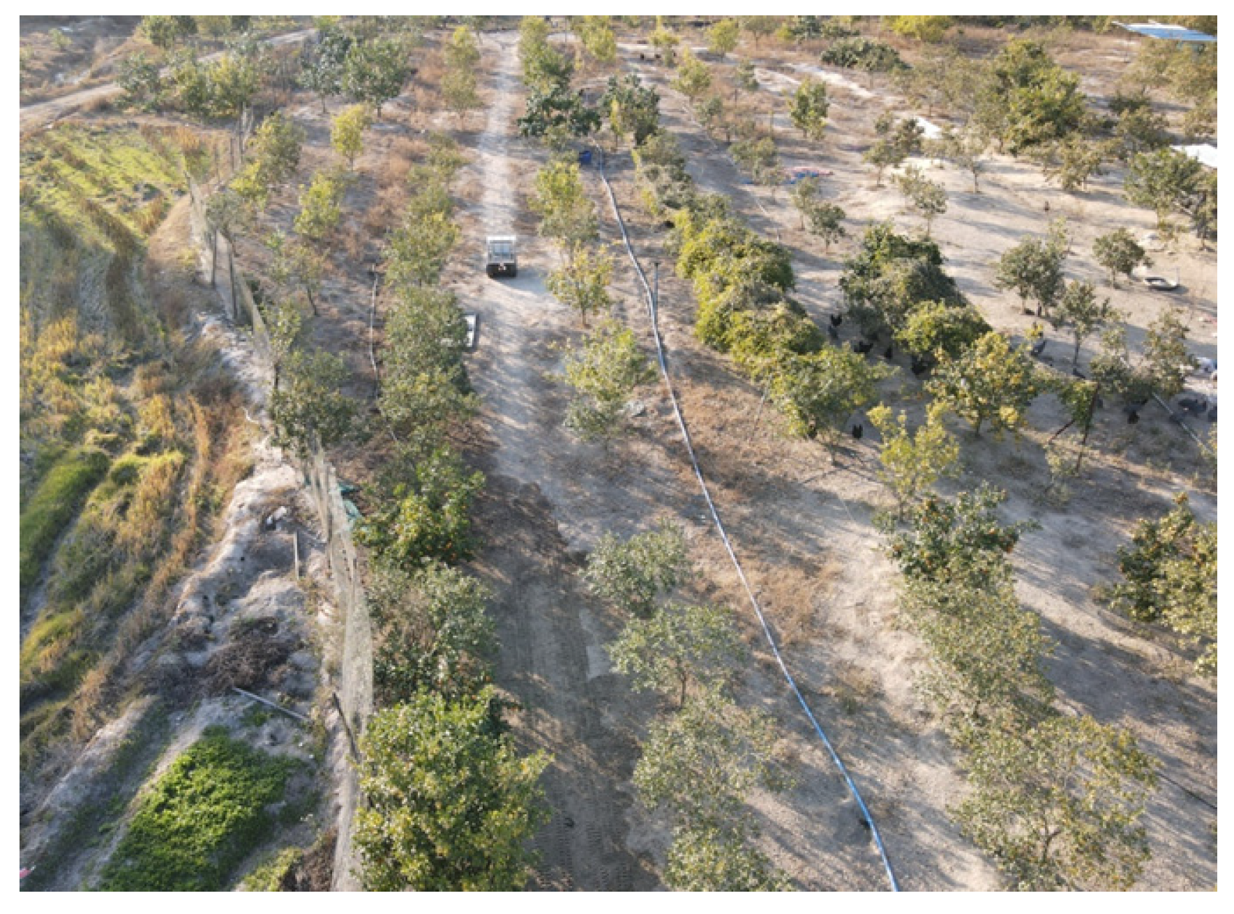
Field experiments were carried out in an orchard environment characterized by uneven terrain and unstructured ground conditions, as illustrated in Figure 5. The test site consists of compacted soil with local undulations, shallow ruts, and mild slopes, which are representative of typical orchard operating scenarios. Such terrain conditions introduce track slip and vehicle posture variations, posing significant challenges for accurate trajectory tracking control.

The experimental area was selected to allow the execution of predefined reference trajectories while avoiding obstacles such as tree trunks and irrigation facilities. During the experiments, the reference trajectories were planned within the available space of the orchard, and different trajectory curvatures were designed to evaluate the tracking performance of the proposed control strategy under varying maneuvering conditions.

All experiments were conducted under similar environmental conditions to ensure fair comparison between different control methods. Vehicle load conditions were adjusted to evaluate the robustness of the proposed NMPC strategy against changes in track–terrain interaction characteristics. The experimental setup provides a realistic test environment for validating the effectiveness and practical applicability of the proposed trajectory tracking control method for tracked agricultural vehicles.

3. Results

3.1. Simulation Results

To evaluate the effectiveness of the improved NMPC strategy with curvature feedforward compensation, simulation experiments were conducted under identical operating conditions. The proposed method was compared with a conventional NMPC approach without curvature feedforward. The evaluation metrics included lateral tracking deviation, heading deviation and optimize solution time.

Simulation parameters are crucial for both simulation experiments and subsequent field experiments. Through literature review and calculations, and by comparing the results of multiple simulation experiments, the optimal simulation parameters were ultimately determined. These parameters are shown in

Table 2. NMPC controller parameters.

NMPC Parameters	Value
Predictive Time Domain Np	12
Control Time Domain Nc	3
Control Cycle (ms)	100
$v_{\mathrm{s},\mathrm{m}\mathrm{a}\mathrm{x}}$	$\pm 0.6 \mathrm{m}/\mathrm{s}$
${\Delta v}_{\mathrm{s},\mathrm{m}\mathrm{a}\mathrm{x}}$	$0.1 \mathrm{m}/\mathrm{s}$
$\varphi$	0.55
Output Tracking Error Weight Q	$\mathrm{d}\mathrm{i}\mathrm{a}\mathrm{g}\left[\mathrm{50,50,10}\right]$
Input amplitude weight R	$\mathrm{d}\mathrm{i}\mathrm{a}\mathrm{g}\left[\mathrm{2,2}\right]$
Input change rate weight P	$\mathrm{d}\mathrm{i}\mathrm{a}\mathrm{g}\left[\mathrm{5,5}\right]$

.

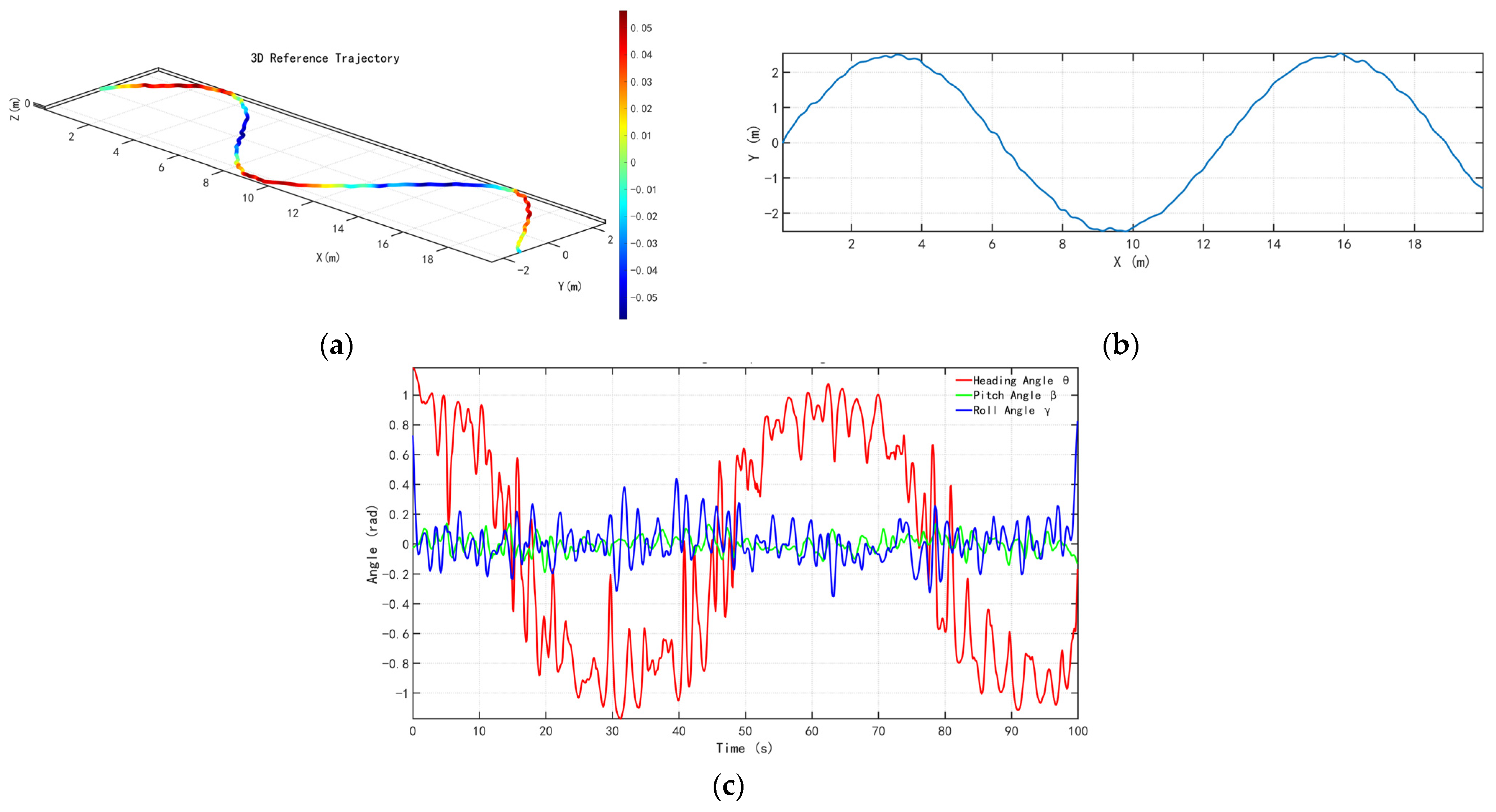
To simulate trajectory tracking tests under real orchard terrain as closely as possible, a three-dimensional target trajectory is defined in MATLAB/Simulink (version R2025b) with artificial noise introduced. The three-dimensional representation in Figure 6a is included to illustrate the terrain-induced height variation along the reference path, which gives rise to the roll and pitch angle variations shown in Figure 6c and justifies the use of the improved three-dimensional kinematic model proposed in Section 2.1.2. The XY-plane projection in Figure 6b is used as the actual reference for trajectory tracking evaluation.

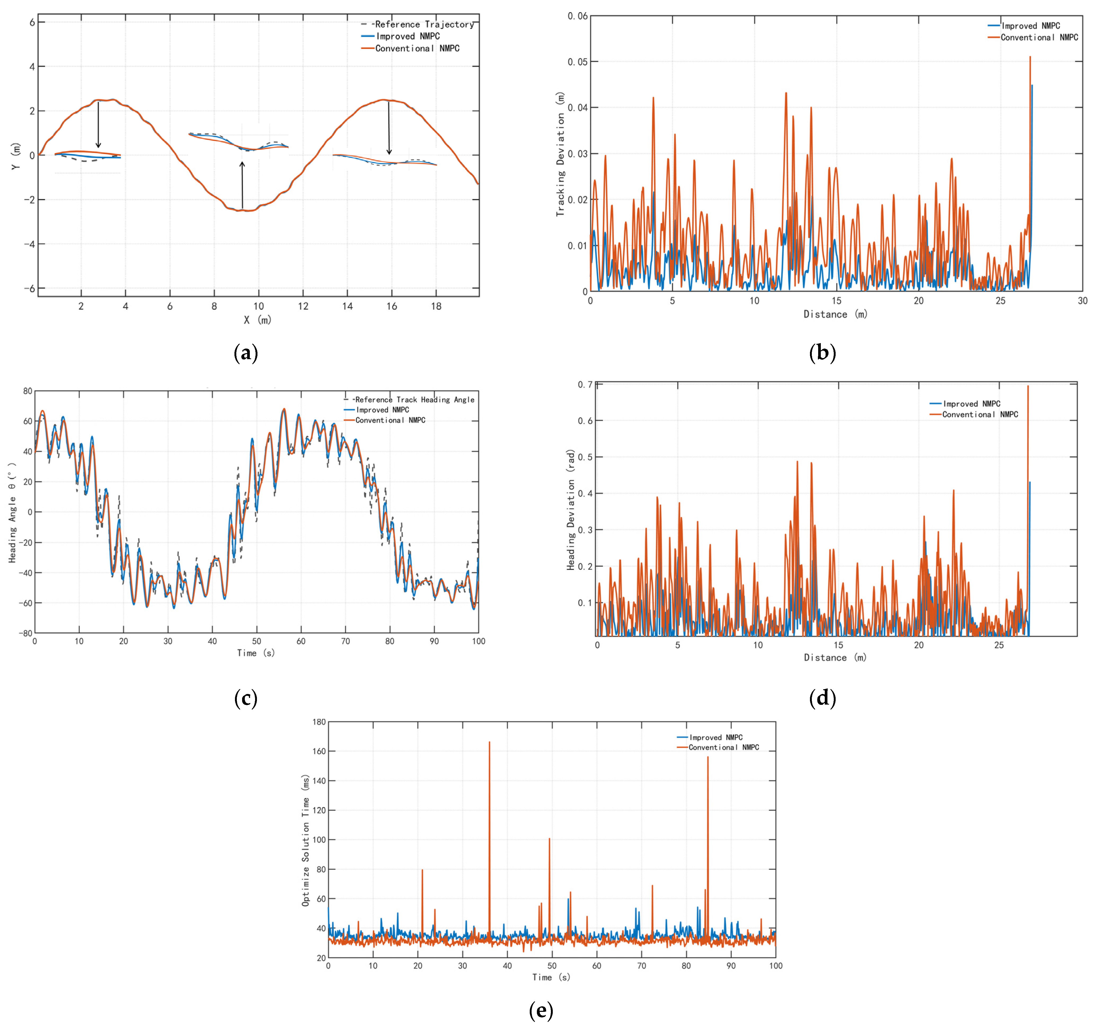
Figure 7 illustrates the trajectory tracking performance of both methods. The proposed approach demonstrates improved tracking accuracy, particularly during curved path segments, where conventional NMPC exhibits noticeable tracking lag. This improvement indicates that the curvature feedforward mechanism enables the controller to respond more proactively to path curvature variations.

Trajectory Tracking Performance and Comparison Diagrams Under Two Control Methods are shown in Figure 7a–d. Compared with conventional NMPC, the proposed method significantly reduces both the magnitude and fluctuation of lateral tracking deviation and heading deviation. Quantitative results summarized in

Table 3. Statistical Table of Trajectory Tracking Performance in Simulation Experiment.

Control Method	Control Indicators	Mean	Standard Deviation	Maximum Value
Improved NMPC	Tracking deviation/cm	0.76	0.52	2.43
	Heading deviation/rad	0.069	0.063	0.44
	Optimize solution time/ms	34.72	2.94	59.87
Conventional NMPC	Tracking deviation/cm	1.09	0.77	5.91
	Heading deviation/rad	0.11	0.097	0.68
	Optimize solution time/ms	31.87	7.12	166.14

indicate that the mean and standard deviation of the lateral tracking deviation are reduced by 30.28% and 32.46%, respectively. Similarly, the mean and standard deviation of the heading deviation are reduced by 37.27% and 35.05% respectively.

Although the response solution time of the improved NMPC is only marginally improved compared to the conventional NMPC, the former ensures that the solver can obtain the optimal solution in a timely manner within each control cycle, thereby avoiding timeouts and enhancing control stability and accuracy. These results demonstrate that the integration of curvature feedforward effectively improves the real-time feasibility of the NMPC controller.

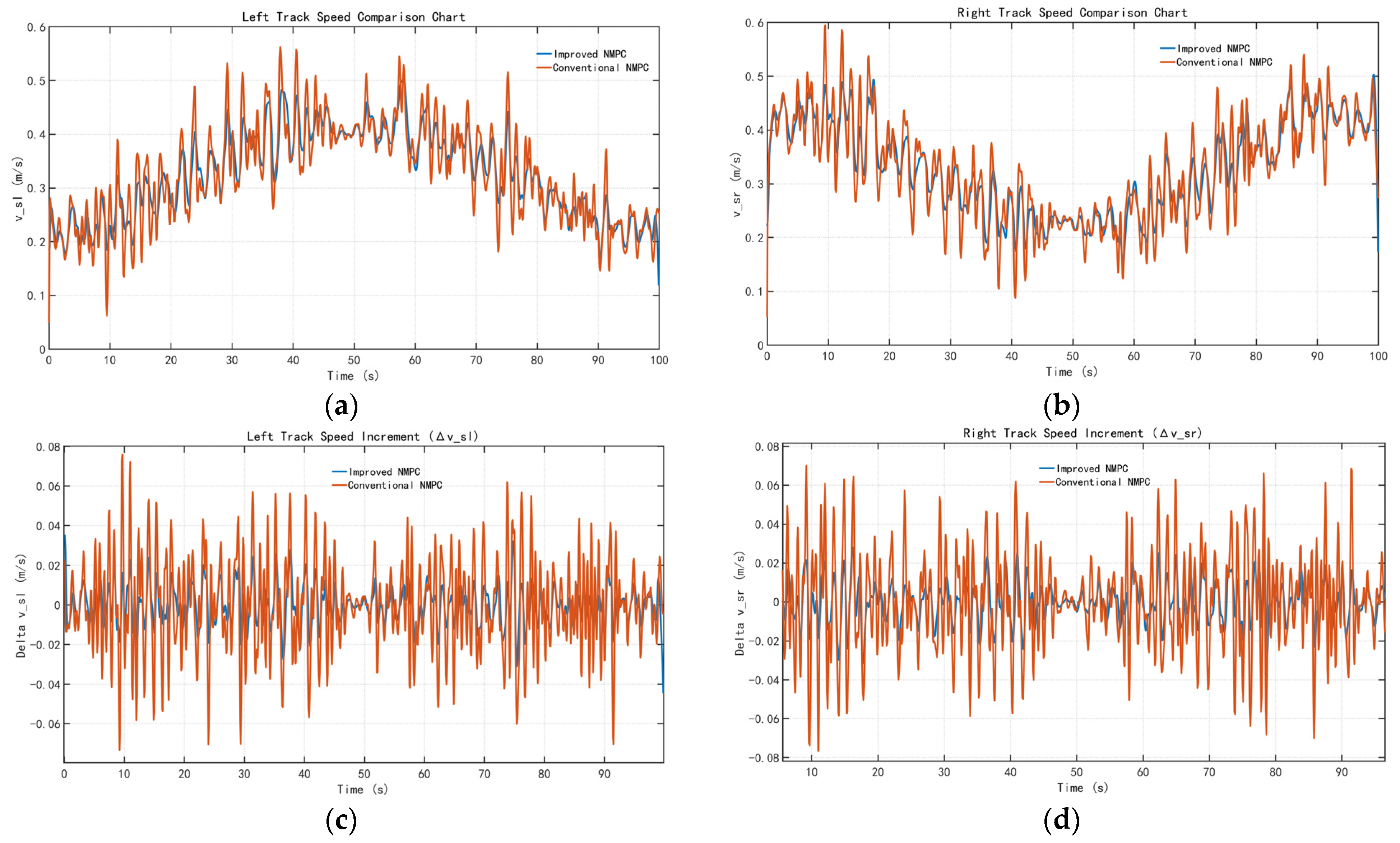
Figure 8 presents the time histories of left and right track velocity commands and their increments under both control methods. As shown in Figure 8a,b, the track velocity commands of both methods remain within the prescribed bounds of ±0.6 m/s throughout the simulation experiment. However, the improved NMPC produces noticeably smoother velocity profiles, whereas conventional NMPC exhibits larger fluctuations particularly during high-curvature segments, which is consistent with the solver timeout behavior reported in Table 3. As shown in Figure 8c,d, both methods satisfy the velocity increment constraint of ±0.1 m/s throughout the experiment. The improved NMPC consistently produces smaller increments, confirming that the curvature feedforward mechanism not only improves tracking accuracy but also enhances the smoothness of control outputs.

3.2. Field Experiment Results

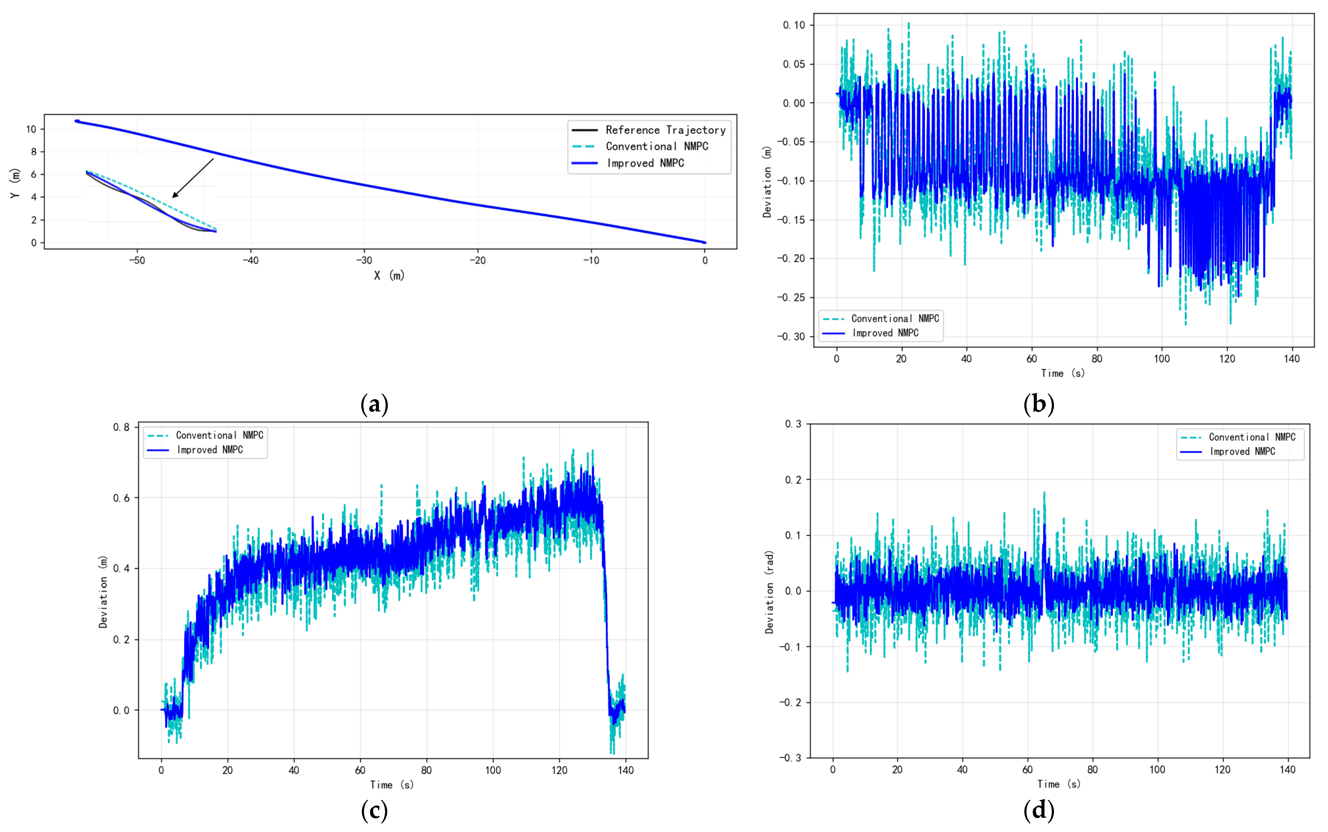
Field experiments were conducted to further validate the proposed control strategy under real agricultural operating conditions. Due to space limitations of the experimental site, custom reference trajectories were designed within the test area. To amplify the influence of track slip and terrain disturbance on trajectory tracking performance, experiments were carried out under three different load conditions: no load, medium load, and heavy load. During real-vehicle validation, since the optimize solution time for each control cycle cannot be accurately obtained as in the simulation phase, the field experiment stage will evaluate the tracking control performance based on three tracking metrics: lateral deviation, longitudinal deviation and heading deviation.

3.2.1. No-Load Condition

Under the no-load condition, the reference trajectory was approximately straight with low curvature. Figure 9 shows the trajectory tracking performance of both control methods. Both the proposed method and conventional NMPC achieve satisfactory tracking performance, with relatively small tracking errors.

Quantitative results summarized in

Table 4. Statistical Table of Trajectory Tracking Performance Under No Load Conditions.

Control Method	Control Indicators	Mean	Standard Deviation	Maximum Value
Improved NMPC	Lateral Deviation (cm)	8.43	5.34	24.92
	Longitudinal Deviation (cm)	40.06	15.52	68.71
	Heading Deviation (rad)	0.023	0.02	0.12
Traditional NMPC	Lateral Deviation (cm)	8.67	5.49	28.51
	Longitudinal Deviation (cm)	41.61	15.85	77.01
	Heading Deviation (rad)	0.032	0.029	0.177

show that the proposed method achieves slight improvements in lateral, longitudinal, and heading errors compared with conventional NMPC. The mean lateral error, longitudinal error, and heading error are reduced by 2.77%, 3.73%, and 28.13%, respectively. The limited performance difference can be attributed to the reduced slip effects and low curvature of the reference trajectory under no-load conditions. As shown in Figure 9a, the improved NMPC maintains closer adherence to the reference trajectory compared with conventional NMPC. Figure 9b,c show that both lateral and longitudinal deviations are relatively small under no-load conditions, which is consistent with the low slip effects and near-straight trajectory in this experiment. Figure 9d confirms that the heading deviation of the improved NMPC is noticeably smaller than that of conventional NMPC throughout the experiment, with a mean reduction of 28.13%.

3.2.2. 50 kg Load Condition

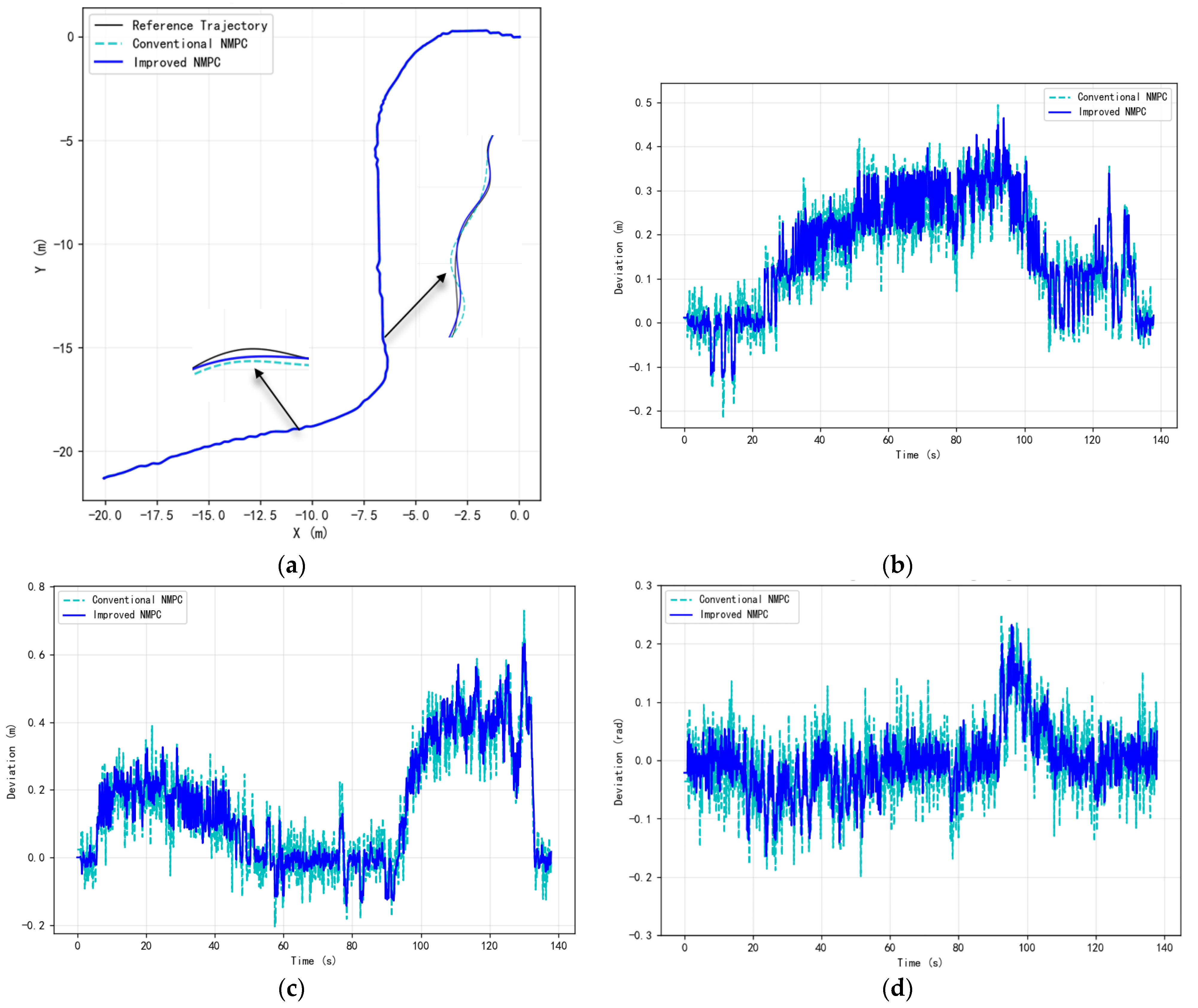
When vehicle load is increased and the reference trajectory becomes more complex, the performance differences between the two methods become more pronounced. Subsequent trials present the trajectory tracking results under loaded conditions. Conventional NMPC exhibits larger tracking deviations, particularly during turning maneuvers, whereas the proposed method maintains closer adherence to the reference trajectory.

As shown in

Table 5. Tracking Performance Statistics Table Under 50 kg Load.

Control Method	Control Indicators	Mean	Standard Deviation	Maximum Value
Improved NMPC	Lateral Deviation (cm)	14.86	10.64	46.21
	Longitudinal Deviation (cm)	14.77	13.52	62.17
	Heading Deviation (rad)	0.042	0.11	0.236
Traditional NMPC	Lateral Deviation (cm)	16.52	11.24	49.97
	Longitudinal Deviation (cm)	16.91	14.74	74.85
	Heading Deviation (rad)	0.054	0.123	0.257

, under medium load conditions, the proposed method reduces the mean lateral error, longitudinal error, and heading error by 10.05%, 12.66%, and 22.22%, respectively, compared with conventional NMPC. Similar performance improvements are observed in the standard deviation and maximum error metrics. As shown in Figure 10a, under 50 kg load conditions, conventional NMPC exhibits more pronounced trajectory deviation particularly during turning maneuvers, whereas the improved NMPC maintains closer tracking of the reference path. Figure 10b,c show that both lateral and longitudinal deviations of the improved NMPC are consistently smaller than those of conventional NMPC. Figure 10d further confirms that the heading deviation is significantly reduced by the proposed method, with a mean reduction of 22.22%.

3.2.3. 100 kg Load Condition

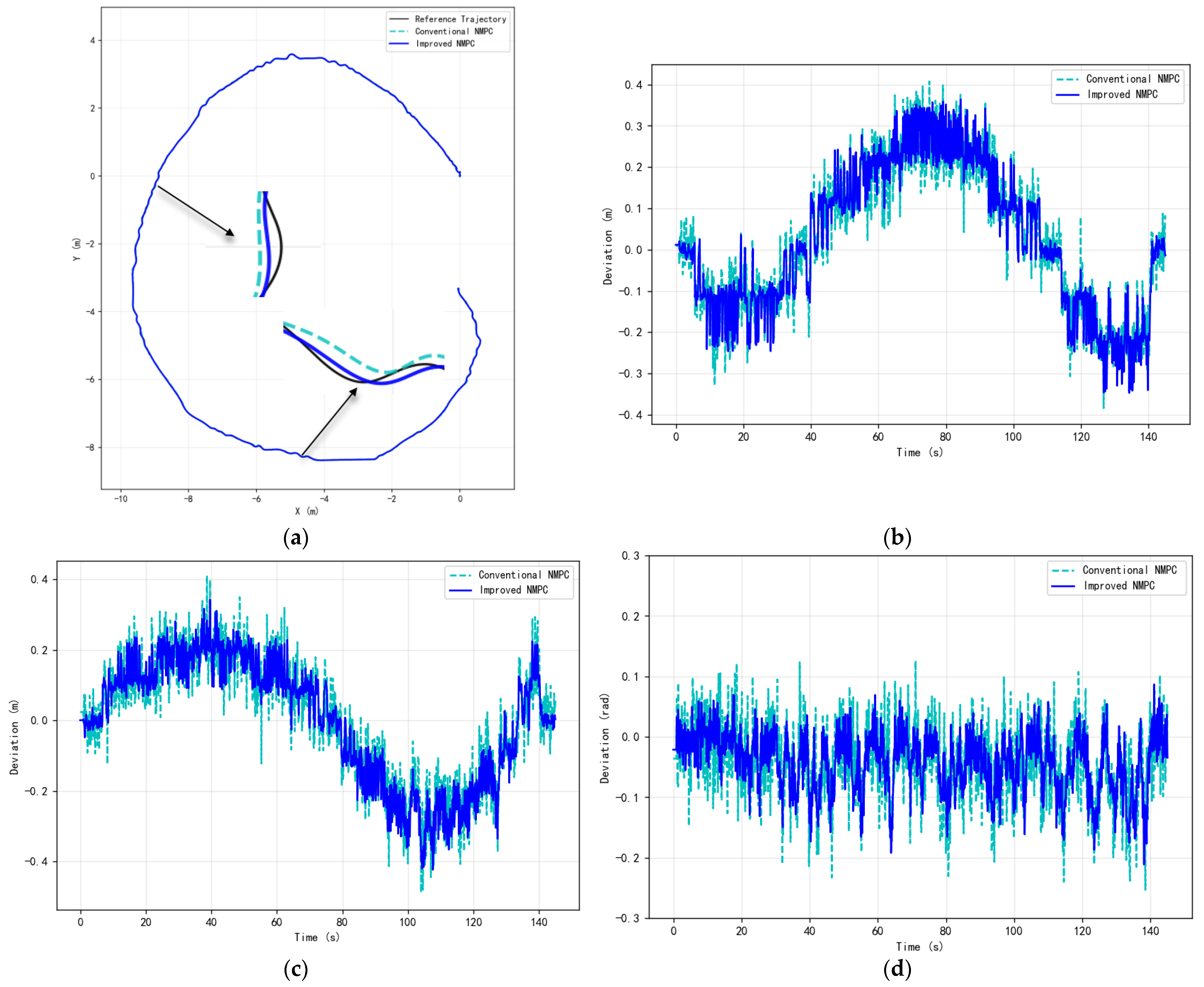
Under the heavy load condition of 100 kg, the reference trajectory was designed with higher curvature to further challenge the control system. Figure 11 shows the trajectory tracking performance of both control methods under this condition. As vehicle load increases and trajectory complexity intensifies, the performance advantage of the improved NMPC becomes increasingly evident compared with conventional NMPC.

Further increasing the vehicle load and trajectory complexity leads to additional performance gains. As summarized in

Table 6. Tracking Performance Statistics Table Under 100 kg Load.

Control Method	Control Indicators	Mean	Standard Deviation	Maximum Value
Improved NMPC	Lateral Deviation (cm)	12.84	8.31	36.36
	Longitudinal Deviation (cm)	12.45	8.3	41.2
	Heading Deviation (rad)	0.05	0.04	0.215
Traditional NMPC	Lateral Deviation (cm)	14.79	9.07	40.88
	Longitudinal Deviation (cm)	14.62	9.16	47.85
	Heading Deviation (rad)	0.06	0.046	0.253

, under heavy load conditions, the proposed method reduces the mean lateral error, longitudinal error, and heading error by 13.18%, 14.84%, and 16.67%, respectively. These results indicate that the proposed control strategy exhibits increased robustness under challenging operating conditions involving higher slip and stronger nonlinear effects. The proposed method maintains stable tracking performance and reduces tracking deviation in high-curvature segments under heavy-load conditions. As shown in Figure 11a, under 100 kg load conditions, the trajectory deviation of conventional NMPC becomes more pronounced, particularly during high-curvature segments, while the improved NMPC continues to track the reference trajectory more accurately. Figure 11b,c demonstrate that the lateral and longitudinal deviations of the improved NMPC are consistently lower than those of conventional NMPC under heavy load conditions. Figure 11d shows that the heading deviation is also effectively reduced, with a mean reduction of 16.67%, confirming the robustness of the proposed control strategy under challenging operating conditions.

3.3. Summary of Results

The simulation and field experiment results consistently demonstrate that the proposed NMPC strategy with curvature feedforward compensation outperforms conventional NMPC in terms of tracking accuracy and computational efficiency. Performance improvements are marginal under ideal conditions with low curvature and minimal slip, but become increasingly significant as vehicle load and trajectory complexity increase. These results confirm the effectiveness of the proposed approach for realistic agricultural operating scenarios.

4. Discussion

The experimental results demonstrate that the proposed curvature-feedforward-enhanced NMPC strategy significantly improves trajectory tracking performance of tracked agricultural vehicles operating under uneven terrain conditions. Compared with conventional NMPC, the proposed method consistently reduces lateral, longitudinal, and heading tracking errors in both simulation and field experiments, while simultaneously improving real-time computational efficiency. These improvements can be attributed to the combined effects of enhanced modeling accuracy and anticipatory feedforward control.

First, the introduction of an improved kinematic model incorporating vehicle roll and pitch angles effectively reduces model mismatch caused by uneven terrain. In orchard environments, terrain undulation and height differences between tracks induce variations in vehicle posture and load distribution, which directly affect track–terrain interaction and vehicle motion behavior. Conventional two-dimensional kinematic models neglect these effects and therefore fail to accurately predict vehicle motion under such conditions. By explicitly accounting for three-dimensional vehicle posture, the proposed model provides more accurate state prediction, which improves NMPC optimization performance and tracking accuracy, particularly under medium to high load conditions.

Second, the online estimation of track slip parameters plays a critical role in enhancing controller robustness. Slip–skid effects are inevitable for tracked vehicles operating on soft soil and uneven terrain, and slip characteristics vary with vehicle load, terrain properties, and operating speed. The proposed Levenberg–Marquardt-based online parameter estimation method allows the prediction model to adapt to time-varying slip conditions, thereby reducing accumulated tracking errors caused by parameter uncertainty. The experimental results indicate that the performance improvement becomes more pronounced as vehicle load and trajectory complexity increase, which further highlights the importance of adaptive slip compensation in realistic agricultural scenarios.

In addition to improved tracking accuracy, the integration of curvature feedforward information significantly enhances the real-time performance of the NMPC controller. Curvature feedforward provides an effective initial control input based on geometric characteristics of the reference trajectory, which reduces the optimization burden of NMPC and mitigates phase lag during turning maneuvers. This effect is particularly evident in scenarios involving high-curvature trajectories, where conventional NMPC may suffer from delayed response or excessive computational cost. The observed reduction in average computation time and its variance confirms that curvature feedforward contributes not only to improved tracking accuracy but also to enhanced control stability and real-time feasibility.

It is important to note that constraint satisfaction is a fundamental requirement for the practical deployment of MPC-based controllers, as infeasibility of the optimization problem can compromise control stability and render the solution physically unrealizable. In the proposed NMPC formulation, two types of inequality constraints are explicitly enforced throughout both simulation and field experiments: control input amplitude constraints ($v_{\mathrm{s},\mathrm{m}\mathrm{a}\mathrm{x}}=\pm 0.6 \mathrm{m}/\mathrm{s}$) and control increment constraints ($\mathsf{\Delta }{v}_{\mathrm{s},\mathrm{m}\mathrm{a}\mathrm{x}}=0.1 \mathrm{m}/\mathrm{s}$), which are derived from the physical characteristics of the drive motors and the ground adhesion conditions, as detailed in Section 2.3.3. The simulation results presented in Figure 8 confirm that the track velocity commands and their increments remain within the prescribed bounds throughout the entire simulation experiment. Both the improved NMPC and conventional NMPC satisfy these constraints during normal operation, while the improved NMPC consistently produces smoother control outputs with smaller velocity fluctuations, as evidenced by the reduced increment magnitudes shown in Figure 8c,d.

To guarantee optimization feasibility under disturbances or modeling mismatch, a slack variable $\epsilon$ is introduced into the NMPC objective function as a soft-constraint mechanism, with a penalty coefficient $\rho >0$. This formulation ensures that the optimization problem always remains feasible even when the vehicle experiences unexpected terrain disturbances or rapid load changes. When the slack variable becomes active, the controller prioritizes feasibility over strict constraint satisfaction, while the feedback optimization loop continues to drive the tracking error toward zero in subsequent control cycles. The penalty coefficient $\rho$ is tuned to be sufficiently large so that the slack variable remains at zero during normal operation, activating only in extreme disturbance scenarios.

The same constraint bounds are applied consistently in the field experiments, and the vehicle successfully completed all experimental trajectories under no-load, 50 kg, and 100 kg load conditions without any motor overload or actuator saturation events, confirming reliable constraint satisfaction across both simulation and real-world operating conditions.

It is noteworthy that the performance improvement achieved by the proposed method is less pronounced under no-load and near-straight trajectory conditions. In such cases, track slip and posture variations are relatively small, and curvature feedforward effects are limited due to low trajectory curvature. Under these conditions, both the proposed method and conventional NMPC can achieve satisfactory tracking performance. However, as operating conditions become more challenging—such as increased vehicle load, more complex trajectories, and uneven terrain—the advantages of the proposed control strategy become increasingly evident. This observation is consistent with the design motivation of the proposed method, which targets realistic agricultural operating scenarios rather than idealized conditions.

Despite the promising results, several limitations of the proposed approach should be acknowledged. First, the slip parameter estimation relies on the accuracy of pose measurements, which may be affected by sensor noise and environmental disturbances. Although high-precision positioning and attitude sensors were employed in this study, further investigation is needed to evaluate the robustness of the proposed method under degraded sensing conditions. Second, the computational complexity of NMPC, while reduced by curvature feedforward, remains higher than that of simple geometric or rule-based controllers. Future work may explore more efficient optimization solvers or learning-based warm-start strategies to further improve real-time performance.

Future research directions include extending the proposed control framework to account for more complex terrain properties, such as varying soil stiffness and moisture content, as well as integrating terrain perception information into the prediction model. In addition, cooperative control strategies involving multiple agricultural vehicles and adaptive trajectory planning under dynamic orchard environments warrant further investigation. These extensions would further enhance the applicability of the proposed method for intelligent and autonomous agricultural operations.

5. Conclusions

This study proposes a nonlinear model predictive control (NMPC) strategy integrated with curvature feedforward compensation for trajectory tracking of tracked agricultural vehicles operating under uneven terrain conditions. Based on simulation and field experiments, the main conclusions can be summarized as follows:

• An improved kinematic modeling framework incorporating vehicle roll and pitch angles was developed to better capture the motion characteristics of tracked agricultural vehicles on uneven terrain. This model reduces prediction errors caused by posture variations and provides a more accurate basis for NMPC trajectory tracking.
• An online slip parameter estimation method based on the Levenberg–Marquardt algorithm was introduced to adaptively compensate for time-varying track slip effects. The proposed estimation strategy improves model adaptability under different load and terrain conditions, thereby enhancing tracking robustness.
• A curvature feedforward mechanism was integrated into the NMPC framework to provide anticipatory control input for path curvature variations. This approach improves tracking accuracy during turning maneuvers and significantly reduces the computational burden of the NMPC optimization process.
• Simulation results demonstrate that the proposed method achieves substantial reductions in lateral and heading tracking errors, as well as optimization computation time, compared with conventional NMPC. Field experiments under different load conditions further confirm that the proposed strategy provides improved tracking performance and robustness in realistic orchard environments.

Overall, the proposed control strategy effectively balances tracking accuracy, robustness, and real-time feasibility, making it suitable for autonomous tracked agricultural vehicles operating in complex and uneven terrain. Future work will focus on incorporating terrain perception information and further improving computational efficiency to enhance adaptability in more diverse agricultural scenarios.

References

1. Zhang, Q.; Pierce, F.J. Agricultural Automation: Fundamentals and Practices; CRC Press: Boca Raton, FL, USA, 2016. [Google Scholar]
2. Bechar, A.; Vigneault, C. Agricultural robots for field operations: Concepts and components. Biosyst. Eng. 2016, 149, 94–111. [Google Scholar] [CrossRef]
3. Shamshiri, R.; Weltzien, C.; Hameed, I.; Yule, I.; Grift, T.; Balasundram, S.; Pitonakova, L.; Ahmad, D.; Chowdhary, G. Research and development in agricultural robotics: A perspective of digital farming. Int. J. Agric. Biol. Eng. 2018, 11, 1–14. [Google Scholar] [CrossRef]
4. Iagnemma, K.; Dubowsky, S. Mobile Robots in Rough Terrain: Estimation, Motion Planning, and Control with Application to Planetary Rovers; Springer Science & Business Media: Berlin/Heidelberg, Germany, 2004. [Google Scholar]
5. Mandow, A.; Martinez, J.L.; Morales, J.; Blanco, J.L.; Garcia-Cerezo, A.; Gonzalez, J. Experimental kinematics for wheeled skid-steer mobile robots. In 2007 IEEE/RSJ International Conference on Intelligent Robots and Systems; IEEE: New York, NY, USA, 2007; pp. 1222–1227. [Google Scholar]
6. Yi, J.; Wang, H.; Zhang, J.; Song, D.; Jayasuriya, S.; Liu, J. Kinematic Modeling and Analysis of Skid-Steered Mobile Robots With Applications to Low-Cost Inertial-Measurement-Unit-Based Motion Estimation. IEEE Trans. Robot. 2009, 25, 1087–1097. [Google Scholar] [CrossRef]
7. Zuo, X.; Zhang, M.; Chen, Y.; Liu, Y.; Huang, G.; Li, M. Visual-inertial localization for skid-steering robots with kinematic constraints. In The International Symposium of Robotics Research; Springer: Berlin/Heidelberg, Germany, 2019; pp. 741–756. [Google Scholar]
8. Chen, Y.; Wu, Y.; Zeng, W.; Du, S. Kinematics Model Estimation of 4W Skid-Steering Mobile Robots Using Visual Terrain Classification. J. Robot. 2023, 2023, 1632563. [Google Scholar] [CrossRef]
9. Ordonez, C.; Gupta, N.; Reese, B.; Seegmiller, N.; Kelly, A.; Collins, E. Learning of skid-steered kinematic and dynamic models for motion planning. Robot. Auton. Syst. 2017, 95, 207–221. [Google Scholar] [CrossRef]
10. Xiong, G.-M.; Lu, H.; Guo, K.-H.; Chen, H.-Y. Research on Trajectory Prediction of Tracked Vehicles Based on Real-Time Slip Estimation. Acta Armamentarii 2017, 38, 600–607. (In Chinese) [Google Scholar] [CrossRef]
11. Wang, F.A.; Yang, Q.H.; Zhang, Z.G.; Li, A.N.; Xu, H.W. Path Tracking and Turning Control Algorithm of Tracked Vehicle Based on ICR. Trans. Chin. Soc. Agric. Mach. 2024, 55, 386–395. (In Chinese) [Google Scholar] [CrossRef]
12. Bussola, R.; Focchi, M.; Zilio, N.; Palopoli, L.; Fontanelli, D. Distributed robot perception for tracked vehicles. In Proceedings of the Italian Conference on Robotics and Intelligent Machines (I-RIM), Roma, Italy, 25–27 October 2024. [Google Scholar]
13. Hu, J.M.; Hu, Y.H.; Chen, H.Y.; Liu, K. Research on Trajectory Tracking of Unmanned Tracked Vehicles Based on Model Predictive Control. Acta Armamentarii 2019, 40, 456–463. (In Chinese) [Google Scholar] [CrossRef]
14. Mayne, D.Q.; Rawlings, J.B.; Rao, C.V.; Scokaert, P.O. Constrained model predictive control: Stability and optimality. Automatica 2000, 36, 789–814. [Google Scholar] [CrossRef]
15. Borrelli, F.; Bemporad, A.; Morari, M. Predictive Control for Linear and Hybrid Systems; Cambridge University Press: Cambridge, UK, 2017. [Google Scholar]
16. Falcone, P.; Borrelli, F.; Asgari, J.; Tseng, H.; Hrovat, D. Predictive active steering control for autonomous vehicle systems. IEEE Trans. Control Syst. Technol. 2007, 15, 566–580. [Google Scholar] [CrossRef]
17. Kayacan, E.; Saeys, W.; Ramon, H.; Belta, C.; Peschel, J. Experimental Validation of Linear and Nonlinear MPC on an Articulated Unmanned Ground Vehicle. IEEE-Asme Trans. Mechatron. 2018, 23, 2023–2030. [Google Scholar] [CrossRef]
18. Katrakazas, C.; Quddus, M.; Chen, W.; Deka, L. Real-time motion planning methods for autonomous on-road driving: State-of-the-art and future research directions. Transp. Res. Part C Emerg. Technol. 2015, 60, 416–442. [Google Scholar] [CrossRef]
19. Liniger, A.; Domahidi, A.; Morari, M. Optimization-based autonomous racing of 1:43 scale RC cars. Optim. Control Appl. Methods 2015, 36, 628–647. [Google Scholar] [CrossRef]
20. Bwambale, E.; Wanyama, J.; Adongo, T.A.; Umukiza, E.; Ntole, R.; Chikavumbwa, S.R.; Sibale, D.; Jeremaih, Z. A review of model predictive control in precision agriculture. Smart Agric. Technol. 2025, 10, 100716. [Google Scholar] [CrossRef]
21. Zhou, B.; Su, X.; Yu, H.; Guo, W.; Zhang, Q. Research on Path Tracking of Articulated Steering Tractor Based on Modified Model Predictive Control. Agriculture 2023, 13, 871. [Google Scholar] [CrossRef]
22. Prado, A.; Torres-Torriti, M.; Yuz, J.; Cheein, F. Tube-based nonlinear model predictive control for autonomous skid-steer mobile robots with tire-terrain interactions. Control Eng. Pract. 2020, 101, 104451. [Google Scholar] [CrossRef]
23. Aro, K.; Guevara, L.; Torres-Torriti, M.; Torres, F.; Prado, A. Robust nonlinear model predictive control for the trajectory tracking of skid-steer mobile manipulators with wheel–ground interactions. Robotics 2024, 13, 171. [Google Scholar] [CrossRef]
24. Gocer, I.; Baslamisli, S. A Slip-Based Model Predictive Control Approach for Trajectory Following of Unmanned Tracked Vehicles. Machines 2025, 13, 817. [Google Scholar] [CrossRef]
25. Cheng, J.; Zhang, B.; Zhang, C.; Zhang, Y.; Shen, G. A model-free adaptive predictive path-tracking controller with PID terms for tractors. Biosyst. Eng. 2024, 242, 38–49. [Google Scholar] [CrossRef]
26. Zhang, T.; Jiao, X.; Lin, Z. Finite time trajectory tracking control of autonomous agricultural tractor integrated nonsingular fast terminal sliding mode and disturbance observer. Biosyst. Eng. 2022, 219, 153–164. [Google Scholar] [CrossRef]
27. Xu, G.; Chen, M.; He, X.; Pang, H.; Miao, H.; Cui, P.; Wang, W.; Diao, P. Path following control of tractor with an electro-hydraulic coupling steering system: Layered multi-loop robust control architecture. Biosyst. Eng. 2021, 209, 282–299. [Google Scholar] [CrossRef]
28. Lin, X.Y.; Jin, Z.W.; Tang, Y.L. Vehicle Lateral Control Strategy Integrating Road Curvature Feedforward. China Mech. Eng. 2025, 36, 2774–2782. (In Chinese) [Google Scholar] [CrossRef]
Figure 1. Dynamics Model of Tracked Vehicles. The teal regions represent the left and right track ground-contact segments, and the purple region represents the vehicle body.
Agriculture 16 00816 g001
Figure 2. Kinematics Model of Tracked Vehicles. The teal regions represent the left and right track ground-contact segments, and the purple region represents the vehicle body.
Agriculture 16 00816 g002
Figure 3. Overall control framework of the proposed curvature-feedforward NMPC strategy.
Agriculture 16 00816 g003
Figure 4. Test Track Vehicle.
Agriculture 16 00816 g004
Figure 5. Aerial view of the experimental orchard environment.
Agriculture 16 00816 g005
Figure 6. (a) Three-dimensional reference trajectory illustrating terrain undulation along the reference path, which motivates the proposed 3D kinematic model; (b) XY-Plane projection of the reference trajectory; (c) Euler angle sequence diagram showing the roll and pitch variations induced by terrain undulation.
Agriculture 16 00816 g006
Figure 7. (a) Comparison diagram of trajectory tracking in the XY-Plane; (b) Tracking deviation comparison chart; (c) Heading tracking comparison chart; (d) Heading deviation comparison chart; (e) Optimize solution time comparison chart.
Agriculture 16 00816 g007
Figure 8. Time histories of track velocity commands and their increments in the simulation experiment: (a) left track velocity v_sl; (b) right track velocity v_sr; (c) left track velocity increment Δv_sl; (d) right track velocity increment Δv_sr. Both methods satisfy the prescribed constraint boundaries ( v s , m a x = ± 0.6   m / s for velocity and Δ v s , m a x = ± 0.1   m / s for increment) throughout the experiment. Both methods satisfy the prescribed constraints throughout the experiment, while the improved NMPC produces smoother control outputs with smaller fluctuations.
Agriculture 16 00816 g008
Figure 9. (a) Tracking effect comparison chart under no load conditions; (b) Lateral deviation timing diagram under no load conditions; (c) Longitudinal deviation timing diagram under no load conditions; (d) Heading deviation timing diagram under no load conditions.
Agriculture 16 00816 g009
Figure 10. (a) Tracking effect comparison chart under 50 kg load; (b) Lateral deviation timing diagram under 50 kg load; (c) Longitudinal deviation timing diagram under 50 kg load; (d) Heading deviation timing diagram under 50 kg load.
Agriculture 16 00816 g010
Figure 11. (a) Tracking effect comparison chart under 100 kg load; (b) Lateral deviation timing diagram under 100 kg load; (c) Longitudinal deviation timing diagram under 100 kg load; (d) Heading deviation timing diagram under 100 kg load.
Agriculture 16 00816 g011