Water and Carbon Footprints of Organic Cotton Under Mediterranean Conditions: Effects of Irrigation Regimes, Cultivar Response, and Carbon Pricing

Abstract

The analysis of water and emission efficiency in cropping systems is vital for sustainable agriculture in Mediterranean regions, which face increasing water shortages. This study offers a site-specific assessment of the Water Footprint (WFP) and Carbon Footprint (CFP) of organic cotton grown under Mediterranean conditions, integrating environmental indicator measurements with economic valuation of greenhouse gas (GHG) emissions via the EU Emissions Trading System (ETS) and the Social Cost of Carbon (SCC). Experiments were carried out at three sites with different soil types, testing two cultivars (Armonia and ST-318) under three irrigation scenarios: severe water deficit (I30), moderate water deficit (I70), and full irrigation (I100). The results reveal significant site-specific variability, with average WFP_lint values ranging from about 1.440 m³ per ton at the most productive site to over 4.100 m³ per ton at the least productive site. Similarly, CFP_lint is lower under high-yield conditions, emphasizing the strong influence of yield on mass-based indicators. At the Carboj and Primosole sites, shifting from (I30) to I100 results in roughly a 50% reduction in emissions, while at Buonfornello, increased irrigation does not consistently produce benefits. The cultivar response is key: Armonia shows greater resilience to water stress, while ST-318 performs best with full irrigation. Overall, the findings highlight that the sustainability of the Mediterranean cotton system depends on factors such as yield performance, site-specific conditions, and cultivar choice.

1. Introduction

Cotton (Gossypium spp.) is cultivated in about 100 countries, with an estimated global production of roughly 24.65 million tons, representing around one-third of natural fiber output [1,2]. Over the next decade, according to OECD and FAO estimates, global raw cotton consumption is expected to grow, driven by population growth and rising incomes in low- and middle-income countries. Global cotton lint production will rise by 1.8% annually, reaching around 28 million tons by 2032, thanks to higher yields (1.4% annually) and expanding cultivated areas (0.4% per year) [3]. Thanks to its unique strengths and versatility, it is often called “white gold” [4], but it also places significant environmental pressure, worsened by the rapid growth of fast fashion, which has made cotton a widely traded commodity [5,6,7]. Although cotton cultivation accounts for only 2.4% (about 1.397 million hectares) of agricultural land and uses only 2.6% of total water withdrawals, this crop is associated with significant environmental impacts on water resources, energy inputs, and agrochemicals [8,9]. This is because roughly 70% of the areas used for its cultivation are under severe water stress [10,11,12]. These impacts are evident in the Mediterranean basin, identified by the IPCC as a “climate change hotspot” [13,14], where, according to estimates, there will be a progressive decrease in water potential of 20–50% by 2070. The need to measure environmental impacts has led to the spread of specific environmental footprint indicators, including the Water Footprint (WFP), which quantifies the water virtually incorporated into the crop cycle through its green WF, blue WF, and grey WF components [15], and the Carbon Footprint (CFP), which quantifies emissions in kg of CO₂e [16]. The debate on the sustainability of the textile industry often compares organic cotton with synthetic fibers, particularly polyester, which is now an alternative to cotton fiber [7]. Specifically, polyester has a Carbon Footprint of 3.7–4.5 t CO₂e per ton of fiber [17,18]. In contrast, estimates of emissions from organic cotton in the main producing countries are around 0.9 kg CO₂e per kg of fiber. This evidence may indicate a potential environmental advantage under certain system boundaries. [19]. Growing attention to these dynamics has led the fashion industry to shift towards sustainability, driven by greater consumer awareness, which is fueling new demand for organic cotton that is mindful of environmental impacts [20]. Although numerous authors [11,19,21,22,23] have analyzed Carbon and Water Footprints internationally, gaps remain in knowledge of site-specific assessments in the Mediterranean environment. Currently, in Italy, cotton cultivation lacks an official statistical framework because of its marginal production [24]. The decline of the crop has been worsened by several economic factors, including low market value (≈1.86 € kg⁻¹) [25], insufficient labor supply, and rising labor costs [26]. This study aims to bridge this knowledge gap by utilizing the experimental results of Vitale et al. (2025) and incorporating data from a third, unpublished study on two cultivars, Armonia and ST-318, subjected to three irrigation regimes (I100, I70, and I30) [23]. Building on this conceptual framework, the analysis addresses the following research questions: 1. How do different irrigation regimes (I100, I70, and I30) affect the green and blue Water Footprint of organic cotton under Mediterranean conditions? 2. How do irrigation levels and cultivar characteristics influence the Carbon Footprint of the cropping system? 3. Do the cultivars Armonia and ST-318 exhibit different environmental responses and resilience to water stress conditions? 4. What is the economic interpretation of the CFP when greenhouse emissions are monetized using the Social Cost of Carbon (SCC) and EU Emissions Trading (ETS) carbon price? [27]. The results should be interpreted within the system boundaries established for this study, which are limited to the cradle-to-farm-gate stage of cotton production. Accordingly, the analysis includes only the agricultural production phase and excludes downstream life cycle stages such as cotton ginning, transport, textile processing, distribution, and final consumption. Furthermore, the results are based on experimental field trials conducted under controlled agronomic conditions, which may differ from those observed in commercial farming systems. Consequently, the outcomes of this study should be understood in the context of the specific experimental conditions and data representativeness, and caution should be exercised when applying these findings to other production systems or agroecological conditions. An additional source of uncertainty is the assumption of a uniform specific energy coefficient for irrigation water across sites, since actual energy demand may vary with local hydraulic and infrastructural conditions.

2. Materials and Methods

2.1. Experimental Structure and Agronomic Management of Experimental Fields

The agronomic data used are derived from experimental trials previously analyzed for agronomic performance. In this work, these data were used to conduct an environmental assessment using Water Footprint and Carbon Footprint indicators.

The analysis was conducted using agronomic data collected from three experimental sites in Sicily during the spring and summer of 2023 and 2024. Site 1 was in the Carboj experimental field (TP) in the Belìce area (37°35′18.0″ N, 12°53′44.0″ E, 65 m above sea level) and managed by the Agricultural Development Agency (ESA) of the Sicilian Region in CastelVetrano. Site 2 was identified at the Primosole Experimental Field (CT) in the Piana di Catania (37°24′ N, 15°03′ E, 10 m above sea level) and managed by the University of Catania. Site 3 was located at the Buonfornello Experimental Field (PA) in Buonfornello (37°58′31″ N, 12°49′07″ E; altitude 10 m above sea level). The chemical and physical properties of the experimental sites are shown in

Table 1. Physical and chemical properties of soils at the three experimental sites.

Soil Characteristic	Unit	Site 1	Site 2	Site 3
Sand	%	59.0	16.6	58
Loam	%	13.0	27.8	13
Clay	%	28.0	55.6	29
Total N	g kg−1	1.30	1.00	2.0
P	mg kg−1	9.16	2.18	10.3
K	mg kg−1	112.9	203.3	103
Organic matter	%	1.46	1.1	1.5
Electrical Conductivity	mS cm−1	0.86	0.15	0.72
CEC	meq %	27.05	14.8	34.5
pH		7.4	7.6	7.9

Sand: sand content in soil (%). Loam: silt content in soil (%). Clay: clay content in soil (%). Total N (g kg⁻¹): total nitrogen content. P (mg kg⁻¹): phosphorus in soil. K (mg kg⁻¹): potassium in soil. Organic matter: organic matter in soil (%). Electrical conductivity (mS cm⁻¹): electrical conductivity. Cation Exchange Capacity (meq %): CEC. pH: soil pH (measured in water). Site 1: Campo Carboj. Site 2: Primosole. Site 3: Buonfornello.

.

The trials used a split-plot design with three replicates. The irrigation volumes were I-100, I-70, and I-30, representing 100%, 70%, and 30% of crop evapotranspiration (ETc). Irrigation volumes were monitored using volumetric flow meters and scheduled based on crop evapotranspiration (ETc), defined as ETc = ETo × Kc, where reference evapotranspiration (ETo) was calculated using the FAO Penman–Monteith equation (

Table 2. Phenological stages, crop coefficients (Kc), and effective rooting depth for cotton according to FAO-56.

Growth Stage	Phenological Description	Kc Range	Effective Rooting Depth (cm)
Initial	Germination: from dry seed to emergence and early seedling development (BBCH 00–09)	0.40–0.50	30
Development	Leaf development: from fully expanded cotyledons to canopy closure (BBCH 10–39)	0.70–0.80	50
Mid-season	Reproductive stage: from first visible flower buds to full boll development (BBCH 51–79)	1.05–1.25	50
Late-season	Senescence: from the onset of leaf senescence to plant maturity and drying (BBCH 91–99)	0.65–0.70	50

) [28]. Irrigation was applied using a self-compensating drip irrigation system (P5^® dripline, Irritec S.p.A., Capo d’Orlando, Italy), with emitters spaced 0.20 m apart and characterized by a nominal flow rate of approximately 2 L h⁻¹ at a pressure of 100 kPa. Irrigation volumes were monitored using volumetric flow meters to accurately quantify the water applied for each irrigation treatment. Differentiated irrigation started after the crop emergence phase was completed, at growth stage BBCH-16. The main plot factor consisted of irrigation levels, while the application of arbuscular mycorrhizal fungi (+AMF vs. −AMF) represented the subplot factor. The microbial bio stimulant Rizoplant (Biogard^®, CBC Europe S.p.A., Grassobbio, Bergamo, Italy) was applied via a fertigation system at two phenological stages (BBCH-13 and BBCH-16). Two cotton cultivars, Armonia and ST-318, were tested in each sub-plot. Each experimental unit covered 16 m² (4 m × 4 m). Meteorological data were collected from stations of the Sicilian Agrometeorological Information Service (SIAS) located near the experimental sites (http://www.sias.regione.sicilia.it—accessed on 10 March 2026) [29]. The stations were equipped with dataloggers and climatic sensors to measure daily minimum and maximum air temperature (°C) and total daily rainfall (mm). These site-specific data were used to define the climatic conditions during the experimental period and to describe the thermos pluviometry trends recorded during the growing seasons (Table 2).

2.2. Methodological Framework for Calculating the Water Footprint

The Water Footprint, including its green (m³ t⁻¹) and blue (m³ t⁻¹) components, was calculated using the definitions and methodological framework of the global standard for water footprint calculation [15]. Choosing the IPCC Tier 1 model to estimate agricultural emissions without conducting a full multi-process LCA aligns with the reference literature [30]. This approach provides a reliable and comparable estimate of emissions, enabling direct comparisons between experimental sites.

2.3. Calculation of the Water Footprint of Cotton

The Water Footprint (WF, m³ t⁻¹) was calculated using a mass-based approach as follows:

$$\mathrm{W}\mathrm{F}\mathrm{P}={\displaystyle \frac{\mathrm{C}\mathrm{W}\mathrm{U}}{\mathrm{Y}}}$$

(1)

where WFP represents the Water Footprint (m³ t⁻¹); CWU indicates crop water use (m³ ha⁻¹), and Y represents fiber yield (t ha⁻¹). The green and blue components of the Water Footprint, expressed in m³ ha⁻¹, were calculated for each experimental treatment as [31,32]:

$${\mathrm{W}\mathrm{F}\mathrm{P}}_{\mathrm{g}\mathrm{r}\mathrm{e}\mathrm{e}\mathrm{n}}={\displaystyle \frac{{\mathrm{C}\mathrm{W}\mathrm{U}}_{\mathrm{g}\mathrm{r}\mathrm{e}\mathrm{e}\mathrm{n}}}{\mathrm{Y}}}$$

(2)

$${\mathrm{W}\mathrm{F}\mathrm{P}}_{\mathrm{b}\mathrm{l}\mathrm{u}\mathrm{e}}={\displaystyle \frac{{\mathrm{C}\mathrm{W}\mathrm{U}}_{\mathrm{b}\mathrm{l}\mathrm{u}\mathrm{e}}}{\mathrm{Y}}}$$

(3)

where CWUgreen and CWUblue denote the green and blue crop water use, defined respectively as the effective use of rainwater stored in the soil and irrigation water withdrawn from surface or groundwater resources (m³ ha⁻¹), and Y represents lint yield (t ha⁻¹). The total Water Footprint (WFP_Total, m³ t⁻¹) was calculated as the sum of the green and blue components, in accordance with ISO 14046 [33]:

$${\mathrm{W}\mathrm{F}\mathrm{T}}_{\mathrm{T}\mathrm{o}\mathrm{t}\mathrm{a}\mathrm{l}}={\mathrm{W}\mathrm{F}}_{\mathrm{g}\mathrm{r}\mathrm{e}\mathrm{e}\mathrm{n}}+{\mathrm{W}\mathrm{F}}_{\mathrm{b}\mathrm{l}\mathrm{u}\mathrm{e}}$$

(4)

This methodological framework follows the mass-based approach commonly applied to annual and fiber crops in Water Footprint assessment studies. In the present experimental organic cotton system, the grey component of the WFP (m³ ha-¹) was not quantified and was excluded from the assessment. The analysis focuses exclusively on the green and blue components of crop water use, representing, respectively, the effective use of rainwater stored in the soil and irrigation water withdrawn from surface or groundwater resources. This choice reflects the scope of this study and the experimental conditions, characterized by the absence of synthetic fertilizers and chemical plant protection products. Under these conditions, the potential pollutant was considered. However, it should be acknowledged that organic systems may still contribute to some nutrient losses, which represent a potential limitation of the approach. Although this assumption is consistent with similar analyses of controller–organic systems, it may limit direct comparability with studies under conventional agricultural management, where grey-water components are explicitly estimated [34].

2.4. Methodological Framework for Calculating the Carbon Footprint

The CF was calculated in accordance with ISO 14067:2018 guidelines [35], using emission factors from the IPCC Sixth Assessment Report (AR6, 2021) and the Ecoinvent v3.9 database (2023) [14,36]. The analysis used a cradle-to-gate system boundary, including all cultivation stages up to harvest. An attributional life cycle assessment approach was employed to determine the Carbon Footprint, aiming to assess the product’s carbon impact and compare its environmental performance; no compensation mechanisms or energy certifications were applied. The mass-based CFP (kg CO₂e kg⁻¹) was derived by normalizing the area-based CFP with respect to crop yield (kg ha⁻¹) (

Table 3. Methodological framework for assessing the Water Footprint and Carbon Footprint of cotton.

Methodological Parameter	Specification
FU	1 t of lint, the main product of the cropping system
Complementary FU	1 kg of cottonseed is considered a co-product
Normalization scale	1 hectare of cultivated area
CFP	Expressed in kg CO2e kg−1
WFP	Expressed in m3 t−1
System boundaries	Cradle to farm gate
Excluded stages	Post-harvest processes, including transport, ginning, and industrial processing

FU: Functional Unit; CFP: Carbon Footprint; WFP: Water Footprint. The main functional unit is 1 t of lint, while 1 kg of cottonseed is considered a complementary co-product. The normalization scale is 1 ha of cultivated area. The CFP was initially calculated on an area basis (kg CO₂e ha⁻¹); later, the area values were normalized relative to the corresponding yields of lint and seed (t ha⁻¹) to obtain emission intensity indicators per unit of mass (kg CO₂e kg⁻¹ of product); WFP is expressed in m³ t⁻¹. Cradle-to-farm gate: the system boundary used.

).

2.5. Calculating the Carbon Footprint of Cotton

The functional unit adopted in this study was 1 ton of cotton lint, selected to ensure a consistent comparison of the environmental impacts associated with the different treatments under investigation. The system boundaries were defined using a cradle-to-farm-gate approach, encompassing all relevant agricultural inputs and field operations up to harvest. Accordingly, the assessment comprised on-farm processes such as soil preparation, sowing, fertilization, irrigation, crop management, and harvesting, whereas downstream life cycle stages, including ginning, transport, textile processing, distribution, and final use, were excluded from the analysis. The estimate included all operational stages, from seedbed preparation to harvesting, and covered the following unit processes: primary and secondary soil preparation (mechanical tillage and harrowing); organic sowing and crop management; irrigation water distribution; electricity used for water pumping and distribution; and diesel used for mechanical field operations. Irrigation volumes were calculated per hectare using the crop water balance approach and the blue crop water requirement (CWU_blue) for each treatment, and the energy used for irrigation was estimated from the distributed water volumes. Greenhouse gas emissions were calculated using characterization factors from the IPCC Sixth Assessment Report (AR6) [37] with 100-year global warming potential (GWP100) values: CO₂ = 1, CH₄ = 27, and N₂O = 273. The modeling of elementary processes within the agricultural supply chain was carried out using the Ecoinvent database [36]. The selected datasets referred to: diesel combustion in agricultural machinery, used to estimate both direct and indirect emissions associated with fuel consumption during mechanical field operations, applying energy-related emission factors expressed in kg CO₂ e L⁻¹; and electricity, medium voltage, Italy, adapted to the national context to account for emissions related to irrigation water pumping and distribution, based on emission factors for electricity production and consumption in Italy [38]. The integration of IPCC AR6 characterization factors and Ecoinvent datasets enabled an updated representation of the climate impacts associated with the main cropping operations for organic cotton at the analyzed sites. As synthetic fertilizers and plant protection products were not applied, soil N₂O emissions were considered negligible or excluded from the Carbon Footprint estimation. The calculation of the Carbon Footprint (CF) followed a formulation commonly adopted in agricultural life cycle assessment (LCA) studies, whereby total emissions are calculated as the sum of the products of consumption of input and their respective emission factors [39]:

$$\mathrm{C}\mathrm{F}\mathrm{P}=\sum (\mathrm{I}\mathrm{n}\mathrm{p}\mathrm{u}\mathrm{t}\mathrm{i}\times \mathrm{E}\mathrm{F}\mathrm{i})$$

(5)

where Inputᵢ denotes the i-th input quantified on a per-hectare basis, and EFᵢ represents the corresponding emission factor (kg CO₂e per unit of input), derived from IPCC AR6 characterization factors and Ecoinvent v3.9 life cycle inventory datasets [36].

2.5.1. Emissions Associated with Irrigation

For irrigation, the emission component was estimated as a function of the electricity consumed by the pumping system, according to the following formulation:

$${\mathrm{C}\mathrm{F}}_{\mathrm{i}\mathrm{r}\mathrm{r}}=\mathrm{E}\_\mathrm{i}\mathrm{r}\mathrm{r}\times \mathrm{F}\mathrm{e}\mathrm{e}\mathrm{l}$$

(6)

where E_irr represents the amount of electricity consumed for irrigation (kWh ha⁻¹), and Feel is the electricity emission factor (kg CO₂e kWh^-1). For the three study sites, a mean specific energy requirement for water equal to 0.45 kWh m⁻³ was assumed, representative of small-scale irrigation systems [40]. This value represents an average coefficient for a pressurized irrigation system and aligns with empirical measurements reported in Mediterranean irrigation districts [41]. This coefficient was applied uniformly across the experimental sites to ensure consistency and comparability in estimating irrigation-related energy use. It is acknowledged, however, that actual energy demand may vary depending on site-specific hydraulic, pedological, and infrastructural conditions, such as pumping depth, hydraulic head, distribution efficiency, and field irrigation characteristics. Since direct site-specific measurements were not available, using a common coefficient was considered an appropriate approximation for the comparative scope of this study, although it remains a source of uncertainty in estimating the irrigation-related Carbon Footprint.

2.5.2. Emissions from Mechanical Operations

Emissions from mechanical operations were estimated by multiplying diesel consumption per hectare (L ha⁻¹) by the relevant emission factor and were calculated as follows:

$${\mathrm{C}\mathrm{F}}_{\mathrm{m}\mathrm{e}\mathrm{c}\mathrm{h}}=\mathrm{F}\mathrm{u}\mathrm{e}\mathrm{l}\times \mathrm{E}\mathrm{F}\_\mathrm{d}\mathrm{i}\mathrm{e}\mathrm{s}\mathrm{e}\mathrm{l}$$

(7)

where Fuel represents diesel consumption (L ha⁻¹), and EF_diesel equals 3.20 kg CO₂e L⁻¹, based on the diesel burned in agricultural machinery dataset from Ecoinvent v3.9. This dataset includes both direct combustion emissions and emissions associated with the entire upstream fuel lifecycle, including extraction, refining, transport, and distribution.

The total emissions were then normalized to the reference functional unit (tons of cotton lint). In this study, greenhouse gas emissions were first calculated at the cropping system level (kg CO₂e ha⁻¹) and subsequently expressed per unit of lint and seed yield as a normalization of system-level emissions relative to productivity. Since the objective was to evaluate the environmental performance of the cultivation system, emissions were not allocated between lint and seed. Mechanical operations were recorded as working hours per hectare and linked to corresponding fuel consumption (

Table 4. Working time and diesel consumption per hectare associated with soil preparation practices in the experimental cotton fields.

Operation	Hours (h ha−1)	Diesel (L h−1)	Diesel Consumption (L ha−1)
Harrowing	6.25	45	7.20
Rotary tillage	3.625	25	6.89

Operation refers to the performed mechanical or agronomic operation; Hours (h ha⁻¹) indicate the working time per hectare; Diesel (L h⁻¹) represents the specific hourly fuel consumption; and Diesel consumption (L ha⁻¹) corresponds to the total diesel consumption per hectare, estimated as the product of working hours and hourly fuel consumption.

).

The analysis was further expanded to include the cotton co-product (cottonseed), providing a complementary assessment of agricultural production-related emission intensity. Cottonseed yield, initially measured at the experimental plot level (g), was converted to kg ha⁻¹ through area-based normalization, using the same method applied for cotton lint, as follows:

$${\mathrm{C}\mathrm{F}\mathrm{P}}_{\mathrm{s}\mathrm{e}\mathrm{e}\mathrm{d}}={\displaystyle \frac{\mathrm{C}\mathrm{F}{\mathrm{P}}_{\mathrm{t}\mathrm{o}\mathrm{t}}}{{\mathrm{Y}}_{\mathrm{s}\mathrm{e}\mathrm{e}\mathrm{d}}}}$$

(8)

where CFP_seed (kg CO2e kg⁻¹ seed) represents the total emissions associated with cottonseed; CFP_total, calculated at the production system level, represents the areal Carbon Footprint of the cropping system (kg CO₂e ha⁻¹); and Y_seed denotes the seed yield (kg ha⁻¹).

The Carbon Footprint (CF) was initially calculated as an aerial system indicator (kg CO₂e ha⁻¹). Starting from this value, and in accordance with ISO 14067:2018 [35], two emission intensity indicators were derived, referring respectively to cotton lint (kg CO₂e kg⁻¹ lint) and cottonseed (kg CO₂e kg⁻¹ seed), obtained by dividing the same areal CFP by the corresponding yields. No allocation procedure was used between cotton lint and cottonseed. Although allocation methods like mass-based or economic allocation are commonly employed in LCA studies of cotton systems, the indicators in this study were calculated separately on a mass basis for each product to maintain a direct link between yield performance, water use, and greenhouse gas emissions under experimental conditions. The results should be interpreted within the defined system boundaries of the study, which are limited to the cradle-to-farm-gate production. Consequently, downstream stages such as transport, processing, and textile manufacturing were not considered in this assessment. Cotton lint was used as the reference functional unit (FU) because it represents the main product of the cotton supply chain and forms the primary basis for comparison with the existing scientific literature. Cottonseed, a secondary co-product, served solely as an additional indicator of emission intensity (kg CO₂e kg seed), calculated by relating the same areal CFP to seed yield without directly attributing emissions to it. This method allows for a broader evaluation of the overall environmental performance of cotton systems across the three experimental sites while ensuring methodological consistency and comparability of results. To evaluate the trade-off between irrigation management and crop productivity, water savings and yield changes were calculated relative to the full-irrigation treatment (I100), which served as the baseline for each site. Water savings (%) were determined by the relative reduction in total water supplied (green and blue components) compared to I100, while yield variation (%) reflected the relative change in productivity levels relative to I100. Negative values indicate yield reductions, whereas positive values indicate yield increases.

2.6. Monetization of the Carbon Footprint: EU ETS and SCC

The cost estimate for carbon emissions was calculated by monetizing the Carbon Footprint (CFP) in metric tons of CO₂e, using two carbon benchmarks [42]. For the EU Emissions Trading System (EU ETS), a rate of €80 per metric ton of CO₂e was used, representing the average market price of emission allowances [43]. Likewise, a rate of €130 per metric ton of CO₂e was applied to the Social Cost of Carbon (SCC), defined as the estimated total economic damage to society from emitting one additional ton of CO₂ [44].

For each treatment, the areal emission cost (€ ha⁻¹) was calculated by multiplying the areal Carbon Footprint (CFP_areal) by the reference CO₂ price (€ t CO₂), as follows:

$${\mathrm{C}}_{\mathrm{h}\mathrm{a}}={\displaystyle \frac{{\mathrm{C}\mathrm{F}\mathrm{P}}_{\mathrm{a}\mathrm{r}\mathrm{e}\mathrm{a}\mathrm{l}}}{1000}}\times \mathrm{P}\mathrm{C}\mathrm{O}$$

(9)

where Cₕₐ represents the areal environmental cost of emissions (€ ha⁻¹); CFP_areal denotes the areal Carbon Footprint (kg CO₂e ha⁻¹); and PCO is the CO₂ price (€ t CO₂), referring either to the EU ETS or the Social Cost of Carbon (SCC):

$$\mathrm{C}\mathrm{e}\mathrm{n}\mathrm{v},\mathrm{p}\mathrm{r}\mathrm{o}\mathrm{d}={\displaystyle \frac{{\mathrm{C}}_{\mathrm{h}\mathrm{a}}}{\mathrm{Y}}}$$

(10)

where Cenv, prod indicates the environmental cost per unit of product (€ t ha⁻¹), and Y is the product yield (t ha⁻¹).

The resulting values were normalized according to crop yields, allowing the determination of environmental costs per unit of product. Both ETS- and SCC-based estimates were expressed as costs per ton of cotton lint (€ t lint) and per ton of cottonseed (€ t seed), by dividing the areal emission cost by the respective yields. In accordance with ISO 14067:2018, this procedure does not allocate emissions between co-products; instead, it normalizes the same areal CFP across different output units, maintaining cotton lint as the reference functional unit and cottonseed as a complementary indicator.

3. Results

3.1. Overall Descriptive Statistics for All Sites

The variability in Water Footprint (WFP) and Carbon Footprint (CFP) indicators, expressed on a mass-based basis for both cotton lint and cottonseed, was quantified using descriptive summary statistics (mean, minimum, maximum, and standard deviation) for each experimental site (

Table 5. Descriptive summary statistics for the three experimental sites.

Site	WFP_Lint (Mean ± SD) m3 t−1	WFP_Lint (Min–Max) m3 t−1	CFP_Lint (Mean ± SD) kg CO2e kg−1	CFP_Lint (Min–Max) kg CO2e kg−1	WFP_Seed (Mean ± SD) m3 t−1	WFP_Seed (Min–Max) m3 t−1	CFP_Seed (Mean ± SD) kg CO2e kg−1	CFP_Seed (Min–Max) kg CO2e kg−1
1	1384 ± 389	898–2178	0.18 ± 0.13	0.05–0.28	874 ± 181	574–1166	0.26 ± 0.02	0.23–0.28
2	2029 ± 824	1167–4896	0.28 ± 0.03	0.24–0.31	1496 ± 443	956–2590	0.28 ± 0.03	0.24–0.31
3	4123 ± 1282	2075–7988	0.30 ± 0.04	0.25–0.35	2960 ± 897	1590–5818	0.30 ± 0.04	0.25–0.35

WFP_lint: Water Footprint of Cotton Lint (m³ t⁻¹); CFP_lint: Carbon Footprint of Cotton Lint (kg CO₂e kg⁻¹); WFP_seed: Water Footprint of Cottonseed (m³ t⁻¹); CFP_seed: Carbon Footprint of Cottonseed (kg CO₂e kg⁻¹); SD: Standard deviation.

).

As shown in Table 5, mean WFP_lint values increased markedly from Site 1 to Site 3 for both cotton lint and cottonseed, with WFP_lint rising from 1384 to 4.123 m³ t⁻¹ and WFP_seed from 874 to 2960 m³ t⁻¹. A similar but less pronounced increase was observed for CFP, with mean CFP, CFP_lint, and CFP_seed reaching their highest values at site 3. Overall, Site 1 had the lowest environmental burdens per unit of product, whereas Site 3 was the most demanding resource

3.2. Water Footprint by Site and Irrigation Regime

3.2.1. Site 1 (Carboj): WFP of Lint and Cottonseed

Under the I30 irrigation regime, total WFP_lint ranged between 1.613 and 2.083 m³ t⁻¹, regardless of treatment and cultivar. The green component (WFP_G_lint) accounted for most of the Water Footprint, with values ranging from 1.487 to 1.920 m³ t⁻¹, while the blue component (WFP_B_lint) contributed less, ranging from 126 to 163 m³ t⁻¹. Under the I70 regime, a decrease in total WFP_lint was observed, with values ranging from 1.100 to 1.419 m³ t⁻¹, while WFP_B_lint increased to between 287 and 370 m³ t⁻¹, indicating a larger contribution from the irrigation component. Under the I100 irrigation regime, WFP_lint had the lowest overall values at Site 1, ranging from approximately 979 to 1.145 m³ t⁻¹. In this case, WFP_G_lint varied from 662 to 775 m³ t⁻¹, while WFP_B_lint ranged from 317 to 371 m³ t⁻¹, confirming a further reduction in the green component and an increase in the blue component as irrigation volumes increase (

Table 6. Green, blue, and total Water Footprint of cotton lint and cottonseed under different irrigation regimes and agronomic treatments at Site 1.

I.	TREATMENT	WFP_G LINT (m3 t−1)	WFP_B LINT (m3 t−1)	WFP_G SEED (m3 t−1)	WFP_B SEED (m3 t−1)	WFP_ TOTAL_LINT (m3 t−1)	WFP_ TOTAL_SEED (m3 t−1)
I30	MIC ARMONIA	1.487	126	938	80	1.613	1.018
	MIC ST-318	1.866	159	1.061	90	2.025	1.152
	NO-MIC ARMONIA	1.596	136	947	81	1.731	1.027
	NO-MIC ST-318	1.920	163	1.041	89	2.083	1.130
I70	MIC ARMONIA	813	287	559	197	1.099	757
	MIC ST-318	877	309	576	203	1.187	779
	NO-MIC ARMONIA	899	317	621	219	1.216	841
	NO-MIC ST-318	1049.1	370	691	244	1.419	935
I100	MIC ARMONIA	662.2	317.0	418.1	200.1	979	618
	MIC ST-318	675.8	323.4	483.3	231.3	999	715
	NO-MIC ARMONIA	774.5	370.7	505.7	242.0	1.145	748
	NO-MIC ST-318	748.5	358.3	576.9	276.1	1.107	853

The green (WFP_G) and blue (WFP_B) components and the total Water Footprint (WFP_Total) of cotton lint and cottonseed (m³ t⁻¹) were evaluated under three irrigation regimes (I30, I70, and I100), two cultivars (Armonia and ST-318), and two treatments (MIC and NO-MIC). The two components are expressed on a mass-based basis, while WFP_Total was calculated as the sum of the green and blue components.

).

Under the I30 irrigation regime, total WFP_seed values ranged approximately between 1.018 and 1.151 m³ t⁻¹, with a clear predominance of the green component (WFP_G_seed), which varied from 938 to 1.061 m³ t⁻¹, while the blue component (WFP_B_seed) contributed to a lesser extent, with values ranging between 80 and 90 m³ t⁻¹. Under the I70 regime, WFP_seed decreased to values ranging between 756 and 935 m³ t⁻¹. In this case, WFP_G_seed ranged from 559 to 691 m³ t⁻¹, whereas WFP_B_seed reached values between 197 and 244 m³ t⁻¹. Under the I100 irrigation regime, WFP_seed reached the lowest values at Site 1, ranging from approximately 618 to 853 m³ t⁻¹. The green component ranged from 418 to 577 m³ t⁻¹, while WFP_B_seed ranged between 200 and 276 m³ t⁻¹ (Table 6).

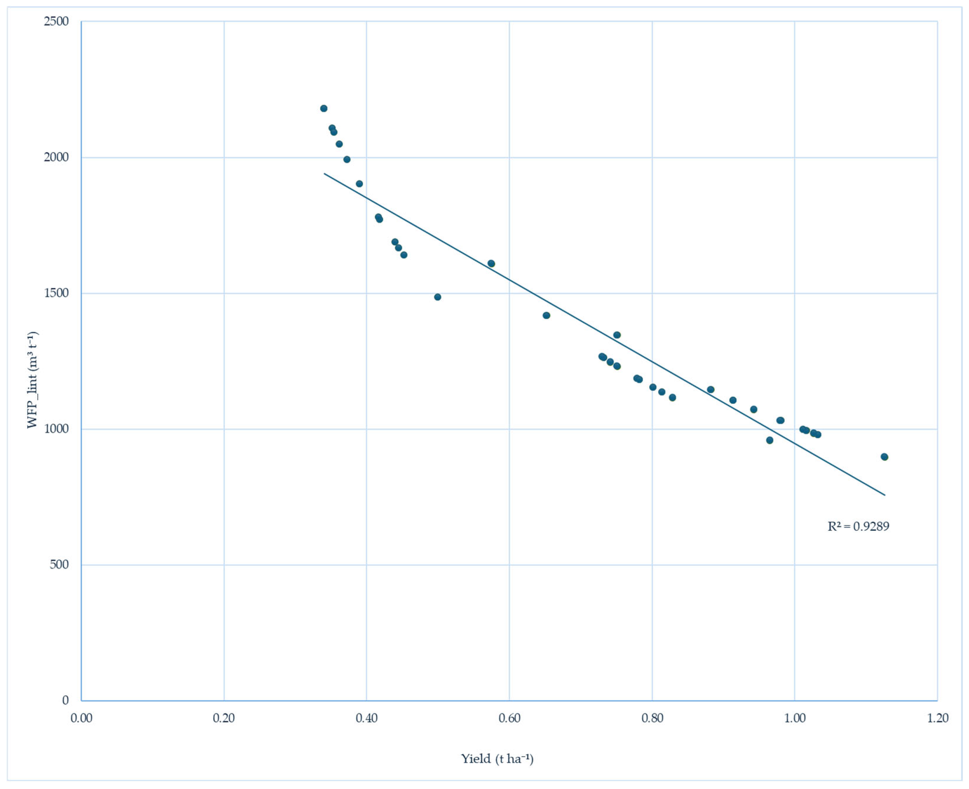
Overall, at Site 1, a consistent reduction in WFP_Total was observed as the irrigation regime increased from I30 to I100 for both products. This trend was accompanied by a change in the Water Footprint composition, marked by a decrease in the green component and a relative increase in the blue component with higher irrigation levels. To support these findings, WFP_lint was further analyzed using linear regression analysis (Figure 1). The analysis showed a strong relationship between the variables, with a very high coefficient of determination (R² ≈ 0.93).

3.2.2. Site 2 (Primosole): WFP of Lint and Cottonseed

Under the I30 irrigation regime, total WFP_lint ranged roughly between 2.467 and 4.045 m³ t⁻¹. The green component (WFP_G_lint) was dominant, with values from 2.251 to 3.691 m³ t⁻¹, while the blue component (WFP_B_lint) contributed less, with values between 216 and 354 m³ t⁻¹. The highest WFP_lint values were seen under NO-MIC treatments, especially for the Armonia cultivar. Under the I70 regime, total WFP_lint decreased to a range of 1.389 to 2.215 m³ t⁻¹, with WFP_G_lint between 1.050 and 1.675 m³ t⁻¹ and WFP_B_lint rising to 338–540 m³ t⁻¹, showing an increased relative contribution of the irrigation component compared to I30. Under the I100 irrigation regime, the lowest WFP_lint values for Site 2 were recorded, ranging from approximately 1.220 to 1.726 m³ t⁻¹. In this case, WFP_G_lint ranged from 818 to 1.157 m³ t⁻¹, while WFP_B_lint varied between 402 and 569 m³ t⁻¹, indicating a reduction in the green component and an increase in the blue component.

A similar pattern was observed for WFP_seed. Under the I30 regime, total WFP_seed ranged between 1.789 and 2.399 m³ t⁻¹, with a clear predominance of the green component, which varied from 1.632 to 2.189 m³ t⁻¹, while WFP_B_seed ranged between 157 and 210 m³ t⁻¹, contributing to a lesser extent. Under the I70 regime, total WFP_seed decreased, with values ranging from 934 to 1.195 m³ t⁻¹, while WFP_B_seed increased to values between 301 and 385 m³ t⁻¹. Under the I100 regime, the lowest WFP_seed values observed at Site 2 were recorded, ranging approximately between 1.037 and 1.153 m³ t⁻¹, with the green component ranging from 695 to 773 m³ t⁻¹ and the blue component between 342 and 380 m³ t⁻¹ (

Table 7. Green, blue, and total Water Footprint of cotton lint and cottonseed under different irrigation regimes and agronomic treatments at Site 2.

I.	TREATMENT	WFP_G LINT (m3 t−1)	WFP_B LINT (m3 t−1)	WFP_G SEED (m3 t−1)	WFP_B SEED (m3 t−1)	WFP_ TOTAL_LINT (m3 t−1)	WFP_ TOTAL_SEED (m3 t−1)
I30	MIC ARMONIA	2.313	222	1.698	163	2.535	1.860
	MIC ST-318	2.251	216	1.632	157	2.467	1.789
	NO-MIC ARMONIA	3.691	354	2.189	210	4.045	2.399
	NO-MIC ST-318	2.358	226	1.740	167	2.585	1.907
I70	MIC ARMONIA	1.050	338	934	301	1.389	1.234
	MIC ST-318	1.289	415	1.106	356	1.704	1.462
	NO-MIC ARMONIA	1.124	362	1.059	341	1.486	1.400
	NO-MIC ST-318	1.675	540	1.195	385	2.215	1.580
I100	MIC ARMONIA	818	402	695	342	1.220	1.037
	MIC ST-318	1.021	502	703	346	1.524	1.049
	NO-MIC ARMONIA	971	478	728	358	1.449	1.087
	NO-MIC ST-318	1.157	569	773	380	1.726	1.153

The green (WFP_G) and blue (WFP_B) components and the total Water Footprint (WFP_Total) of cotton lint and cottonseed (m³ t⁻¹) under three irrigation regimes (I30, I70, and I100), two cultivars (Armonia and ST-318), and two treatments (MIC and NO-MIC). The two components are expressed on a mass-based basis, while WFP_Total is calculated as the sum of the green and blue components.

).

3.2.3. Site 3 (Buonfornello): WFP of Lint and Cottonseed

Under the I30 irrigation regime, total WFP_lint ranged between 3.365 and 4.108 m³ t⁻¹. The green component (WFP_G_lint) showed high values, ranging from 2.841 to 3.468 m³ t⁻¹, while the blue component (WFP_B_lint) contributed substantially, with values between 524 and 640 m³ t⁻¹. The highest WFP_lint values were observed for the ST-318 cultivar, whereas lower values were recorded for the mycorrhizal treatment of the Armonia cultivar. Under the I70 regime, total WFP_lint ranged between 2.589 and 4.215 m³ t⁻¹. In this case, WFP_G_lint varied from 1.659 to 2.695 m³ t⁻¹, while WFP_B_lint increased markedly, ranging between 933 and 1.519 m³ t⁻¹, resulting in a significant increase in the blue component compared to the I30 regime. Under the I100 irrigation regime, the highest total WFP_lint values were recorded, ranging between 3.548 and 5.728 m³ t⁻¹. In this regime, WFP_G_lint ranged from 1.904 to 3.073 m³ t⁻¹, while WFP_B_lint reached values between 1.644 and 2.654 m³ t⁻¹, highlighting a marked increase in the irrigation-related component.

A similar trend was observed for WFP_seed. Under the I30 regime, total WFP_seed ranged approximately between 2.501 and 3.253 m³ t⁻¹, with a clear predominance of the green component, which varied from 2.112 to 2.747 m³ t⁻¹, while the blue component ranged between 389 and 507 m³ t⁻¹. Under the I70 regime, total WFP_seed ranged between 2.025 and 3.027 m³ t⁻¹, with the green component varying from 1.295 to 1.936 m³ t⁻¹ and the blue component, which increased substantially, ranging between 730 and 1.091 m³ t⁻¹. The I100 regime exhibited the highest WFP_seed values observed at Site 3, with a range between approximately 2.556 and 4.243 m³ t⁻¹. In this case, the green and blue components ranged from 1.372 to 2.276 m³ t⁻¹ and from 1.185 to 1.966 m³ t⁻¹, respectively (

Table 8. Green, blue, and total Water Footprint of cotton lint and cottonseed under different irrigation regimes and agronomic treatments at Site 3.

I.	TREATMENT	WFP_G LINT (m3 t−1)	WFP_B LINT (m3 t−1)	WFP_G SEED (m3 t−1)	WFP_B SEED (m3 t−1)	WFP_ TOTAL_LINT (m3 t−1)	WFP_ TOTAL_SEED (m3 t−1)
I30	MIC ARMONIA	2841	524	2747	507	3365	3253
	MIC ST-318	3468	640	2501	461	4108	2963
	NO-MIC ARMONIA	2962	546	2112	389	3508	2501
	NO-MIC ST-318	3229	595	2332	430	3825	2762
I70	MIC ARMONIA	2669	1504	1796	1012	4173	2808
	MIC ST-318	2695	1519	1856	1046	4215	2902
	NO-MICARMONIA	1656	933	1295	730	2589	2025
	NO-MIC ST-318	2667	1503	1936	1091	4171	3027
I100	MIC ARMONIA	3073	2654	2276	1966	5728	4242
	MIC ST-318	2735	2363	1825	1576	5098	3401
	NO-MIC ARMONIA	1904	1644	1372	1185	3548	2556
	NO-MIC ST-318	2760	2384	1649	1424	5144	3073

The green (WFP_G) and blue (WFP_B) components and the total Water Footprint (WFP_Total) of cotton lint and cottonseed (m³ t⁻¹) under three irrigation regimes (I30, I70, and I100), two cultivars (Armonia and ST-318), and two treatments (MIC and NO-MIC). The two components are expressed on a mass-based basis, while WFP_Total is calculated as the sum of the green and blue components.

).

3.3. Carbon Footprint (CFP) by Site and Irrigation Regime

3.3.1. Site 1 (Carboj) of Lint and Cottonseed

Across Sites 1, 2, and 3, the Carbon Footprint (CFP) of cotton (kg CO₂e kg⁻¹) for both lint and cottonseed showed systematic variability across irrigation regimes, microbial treatments, and cultivars.

Under the I30 irrigation regime, CFP_lint values ranged between 0.51 and 0.66 kg CO₂e kg⁻¹. The lowest values were observed for the MIC Armonia treatments (0.51 kg CO₂e kg⁻¹), whereas the highest values were recorded under NO-MIC ST-318 treatments (0.66 kg CO₂e kg⁻¹). Overall, NO-MIC treatments exhibited higher CFP_lint values compared to the corresponding mycorrhizal treatments. Under the I70 regime, a reduction in CFP_lint was observed, with values ranging between 0.317 and 0.409 kg CO₂e kg⁻¹. The minimum values were associated with the MIC Armonia treatment (0.317 kg CO₂e kg⁻¹), while the maximum values were again observed for NO-MIC ST-318 (0.409 kg CO₂e kg⁻¹). The I100 irrigation regime yielded the lowest CFP_lint values recorded at Site 1, ranging from 0.27 to 0.32 kg CO₂e kg⁻¹. Also, under full irrigation, MIC treatments consistently performed better than NO-MIC treatments, while the ST-318 cultivar generally exhibited higher CFP_lint values than Armonia.

A similar pattern was observed for CFP_seed. Under the I30 regime, values ranged between 0.32 and 0.36 kg CO₂e kg⁻¹, with lower values consistently associated with MIC treatments. Under the I70 regime, CFP_seed decreased, falling within the range of 0.218–0.269 kg CO₂eCO₂e kg⁻¹. The lowest value (0.218 kg CO₂e kg⁻¹) was observed for MIC Armonia, whereas the highest value (0.269 kg CO₂e kg⁻¹) was recorded under NO-MIC ST-318. Under the I100 regime, CFP_seed reached its lowest values, ranging between 0.175 and 0.225 kg CO₂e kg⁻¹. At this irrigation intensity, MIC treatments showed lower CFP_seed values than the corresponding NO-MIC treatments in both cultivars. The combined CFP_lint seed under the I30 regime ranged between 0.831 and 1.105 kg CO₂e kg⁻¹. Under the I70 and I100 regimes, this indicator decreased, falling within ranges of 0.535–0.678 kg CO₂e kg⁻¹ and 0.445–0.548 kg CO₂e kg⁻¹, respectively (

Table 9. Site 1—Carbon Footprint (CFP) of cotton lint and cottonseed, and total CFP (lint + seed) of organic cotton as a function of irrigation regime and microbial treatment (MIC and NO-MIC).

I.	TREATMENT	CF_Lint CO2e kg−1	CF_Seed CO2e kg−1	CFP_Lint Seed CO2e kg−1
I30	MIC ARMONIA	0.51	0.32	0.83
	MIC ST-318	0.64	0.36	1.00
	NO-MIC ARMONIA	0.55	0.32	0.87
	NO-MIC ST-318	0.66	0.36	1.02
I70	MIC ARMONIA	032	0.22	0.54
	MIC ST-318	0.34	0.22	0.57
	NO-MIC ARMONIA	0.35	0.24	0.59
	NO-MIC ST-318	0.41	0.27	0.68
I100	MIC ARMONIA	0.27	0.18	0.45
	MIC ST-318	0.29	0.18	0.47
	NO-MIC ARMONIA	0.30	0.21	0.51
	NO-MIC ST-318	0.32	0.23	0.55

I.: irrigation regime (I30 = severe deficit irrigation; I70 = moderate deficit irrigation; and I100 = full irrigation); treatment: MIC and NO-MIC. CFP_lint and CFP_seed denote the Carbon Footprint expressed on a mass-based basis, while CFP_lint seed represents the sum of the lint and seed components.

).

3.3.2. Site 2: CFP of Lint and Cottonseed

Under the I30 irrigation regime, CFP_lint values ranged between 0.547 and 0.897 kg CO₂e kg⁻¹. The lowest values were recorded under mycorrhizal treatments (MIC Armonia: 0.562 kg CO₂e kg⁻¹; MIC ST-318: 0.547 kg CO₂e kg⁻¹), whereas the highest value was observed for the NO-MIC Armonia treatment (0.897 kg CO₂e kg⁻¹). The NO-MIC ST-318 treatment showed intermediate values (0.573 kg CO₂e kg⁻¹). Under the I70 regime, CFP_lint decreased markedly, falling within the range of 0.298–0.474 kg CO₂e kg⁻¹. The minimum value was observed for MIC Armonia (0.298 kg CO₂e kg⁻¹), whereas the maximum value was associated with NO-MIC ST-318 (0.474 kg CO₂e kg⁻¹). The I100 irrigation regime resulted in the lowest CFP_lint values, ranging from 0.256 to 0.362 kg CO₂e kg⁻¹.

Under the I30 regime, CFP_seed values ranged between 0.397 and 0.532 kg CO₂e kg⁻¹, with lower values under MIC treatments and higher values under NO-MIC treatments, particularly for the Armonia cultivar. Under the I70 regime, CFP_seed decreased, with values of 0.252 kg CO₂e kg⁻¹ for MIC Armonia and 0.338 kg CO₂e kg⁻¹ for NO-MIC ST-318. Under the I100 regime, CFP_seed reached its lowest values, ranging between 0.217 and 0.242 kg CO₂e kg⁻¹, with the best performance consistently observed under MIC treatments for both cultivars. Considering the combined CFP_lint seed, values under the I30 regime ranged from 0.944 to 1.429 kg CO₂e kg⁻¹, with the highest value observed for the NO-MIC Armonia treatment. Under the I70 regime, CFP_lint seed decreased, ranging between 0.550 and 0.812 kg CO₂e kg⁻¹. The lowest emission values were observed under the I100 regime, ranging between 0.473 and 0.604 kg CO₂e kg⁻¹ (

Table 10. Site 2—Carbon Footprint (CFP) of organic cotton lint and cottonseed, and total CFP, as a function of irrigation regime and mycorrhizal treatment.

I.	TREATMENT	CF_Lint CO2e kg−1	CF_Seed CO2e kg−1	CFP_Lint Seed CO2e kg−1
I30	MIC ARMONIA	0.56	0.41	0.97
	MIC ST-318	0.54	0.39	0.94
	NO-MIC ARMONIA	0.89	0.53	1.42
	NO-MIC ST-318	0.57	0.42	0.99
I70	MIC ARMONIA	0.29	0.25	0.55
	MIC ST-318	0.36	0.31	0.67
	NO-MIC ARMONIA	0.31	0.29	0.61
	NO-MIC ST-318	0.47	0.33	0.81
I100	MIC ARMONIA	0.25	0.21	0.47
	MIC ST-318	0.31	0.22	0.53
	NO-MIC ARMONIA	0.30	0.22	0.53
	NO-MIC ST-318	0.36	0.24	0.60

I.irrigation regime (I30 = severe deficit irrigation; I70 = moderate deficit irrigation; and I100 = full irrigation); treatment: MIC and NO-MIC. CFP_lint and CFP_seed denote the Carbon Footprint expressed on a mass-based basis, while CFP_Total represents the sum of the lint and seed components.

).

Overall, at Site 2, CFP decreased progressively from the I30 to the I100 irrigation regime, with systematic differences observed between MIC and NO-MIC treatments and between the two cultivars.

3.3.3. Site 3: CFP of Lint and Cottonseed

The higher CFP_ lint values observed at Site 3 under the I100 irrigation regime should be interpreted in relation to the yield performance recorded at this site. Because Carbon Footprint indicators are expressed on a mass basis (kg CO₂e t⁻¹), lower yields increase the footprint intensity even when total emissions remain relatively similar. Therefore, the pattern observed at Site 3 mainly reflects a yield-driven effect rather than a direct increase in emissions associated with irrigation inputs.

Under the I30 irrigation regime, CFP_lint values ranged between 0.878 and 1.071 kg CO₂e kg⁻¹. The lowest value was observed for MIC Armonia (0.878 kg CO₂e kg⁻¹), whereas the highest value was recorded for MIC ST-318 (1.071 kg CO₂e kg⁻¹). NO-MIC treatments showed intermediate values, ranging between 0.915 and 0.997 kg CO₂e kg⁻¹. Under the I70 regime, CFP_lint ranged between 0.622 and 1.012 kg CO₂e kg⁻¹. The minimum value was recorded for NO-MIC Armonia (0.622 kg CO₂e kg⁻¹), while the highest values were observed for MIC Armonia and MIC ST-318 (1.002 and 1.012 kg CO₂e kg⁻¹, respectively). Under the I100 regime, CFP_lint reached the highest values observed at Site 3, ranging between 0.815 and 1.316 kg CO₂e kg⁻¹. The maximum value corresponded to MIC Armonia (1.316 kg CO₂e kg⁻¹), while the minimum value was recorded under NO-MIC treatment (0.815 kg CO₂e kg⁻¹).

A similar pattern was observed for CFP_seed. Under the I30 regime, values ranged between 0.652 and 0.849 kg CO₂e kg⁻¹, with the highest value observed for MIC Armonia (0.849 kg CO₂e kg⁻¹). Under the I70 regime, CFP_seed ranged between 0.486 and 0.727 kg CO₂e kg⁻¹. The lowest value was recorded for NO-MIC Armonia (0.486 kg CO₂e kg⁻¹), while the highest value was observed for NO-MIC ST-318 (0.727 kg CO₂e kg⁻¹). The combined CFP_lint seed under the I30 regime ranged between 1.567 and 1.844 kg CO₂e kg⁻¹. Under the I70 regime, emissions varied between 1.108 kg CO₂e kg⁻¹ (NO-MIC Armonia) and 1.728 kg CO₂e kg⁻¹. Under the I100 regime, values ranged from 1.402 to 2.291 kg CO₂e kg⁻¹, with the highest observed for MIC Armonia. Overall, at Site 3, CFP values for both cotton lint and cottonseed were consistently high across all irrigation regimes, with substantial variability among cultivars and microbial treatments (

Table 11. Site 3—Carbon Footprint (CFP) of organic cotton lint and cottonseed, and CFP_Total, as a function of irrigation regime and mycorrhizal treatment.

I.	TRAETMENT	CF_Lint CO2e kg−1	CF_Seed CO2e kg−1	CFP_Total CO2e kg−1
I30	MIC ARMONIA	0.87	0.84	1.72
	MIC ST-318	1.07	0.77	1.84
	NO-MIC ARMONIA	0.91	0.65	1.56
	NO-MIC ST-318	0.99	0.7	1.71
I70	MIC ARMONIA	1.00	0.67	1.67
	MIC ST-318	1.01	0.69	1.70
	NO-MIC ARMONIA	0.62	0.48	1.10
	NO-MIC ST-318	1.00	0.72	1.72
I100	MIC ARMONIA	1.31	0.97	2.29
	MIC ST-318	1.17	0.78	1.95
	NO-MIC ARMONIA	0.81	0.58	1.40
	NO-MIC ST-318	1.18	0.70	1.88

I.: irrigation regime (I30 = severe deficit; I70 = moderate deficit; I100 = full irrigation); treatment = MIC and NO-MIC; CFP_lint and CFP_seed = mass-based Carbon Footprint; CFP_total = sum of the lint and seed components.

).

It should be noted that mass-based indicators are strongly influenced by crop yield. Consequently, higher footprint values per unit of product may occur in lower-productivity situations, even when total resource use per hectare remains comparable. This effect partly explains the higher WFP and CFP values observed at Site 3, where lint yields were lower than those recorded at the other experimental site. Compared with full irrigation (I100), moderate (I70) and severe deficit (I30) irrigation regimes resulted in water savings ranging from 9% to 36% across sites. Yield response exhibited marked site-specific variability: under I30, yield reductions ranged between 25% and 61%, whereas under I70, yield losses were more limited (approximately 21%) at Sites 1 and 2. In contrast, at Site 3, an increase in yield (+9%) was observed under the I70 regime (

Table 12. Water savings and lint yield variation relative to full irrigation (I100) under the I30 and I70 irrigation regimes across the three experimental sites.

Site	Irr.	Total (m3 t−1)	Water Saving (%) vs. I100	Lint Yield (t ha−1)	Yield Change (%) vs. I100
Site 1	I30	741.5	27	0.40	−58
	I70	924.4	9	0.76	−21
	I100	1010.5		0.96
Site 2	I30	1085.0	27	0.39	−61
	I70	1308.9	11	0.79	−21
	I100	1476.9		1.01
Site 3	I30	959.30	36	0.25	−25
	I70	1266.6	16	0.36	9
	I100	1509.7		0.33

Site: experimental site; Irr.: irrigation regime (I30, I70, and I100); total (m³ t⁻¹): total water FP per unit of lint; water saving (%) vs. I100: water saving relative to full irrigation; lint yield (t ha⁻¹): lint yields; yield change (%) vs. I100: yields variation relative to full irrigation.

).

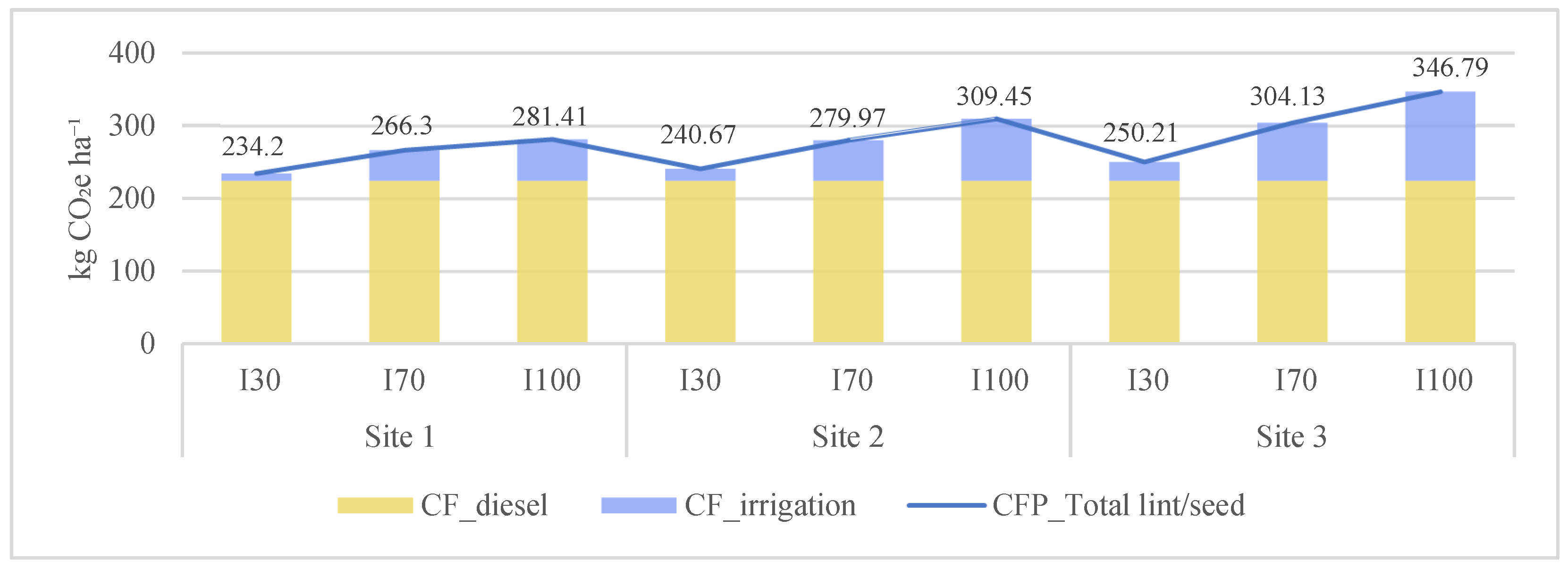
Across all sites and irrigation regimes, CF_diesel represented the dominant emission component, with stable values along the irrigation gradient. In contrast, the contribution of irrigation increased from I30 to I100, resulting in a progressive increase in CFP_Total. At Site 1, CFP_Total increased from 234.2 kg CO₂e ha⁻¹ under I30 to 266.3 kg CO₂e ha⁻¹ under I70, reaching 281.4 kg CO₂e ha⁻¹ under I100. A similar pattern was observed at Site 2, where CFP_Total increased from 240.7 kg CO₂e ha⁻¹ under I30 to 309.45 kg CO₂e ha⁻¹ under I100. Site 3, characterized by overall higher values, exhibited CFP_Total ranging from 250.2 kg CO₂e ha⁻¹ under I30 to 346.8 kg CO₂e ha⁻¹ under I100. Overall, Figure 2 shows a systematic increase in CFP_Total from Site 1 to Site 3, with a consistent effect of the irrigation regime, primarily driven by the energy-related component of irrigation.

3.4. Monetization of Emissions: ETS and SCC

3.4.1. Site 1

Table 13. Site 1—ETS and SCC monetization of the Carbon Footprint of cotton lint and cottonseed as a function of irrigation regime and agronomic treatment (MIC and NO-MIC).

I.	TREATMENT	ETS_Lint	ETS_Seed	ETS_Lint-Seed	SCC_Lint	SCC_Seed	SCC_Lint-Seed
I30	MIC ARMONIA	40.8	25.7	66.5	66.2	41.8	108.0
	MIC ST-318	51.2	29.1	80.3	83.1	47.3	130.4
	NO-MIC ARMONIA	43.7	26.0	69.7	71.1	42.2	113.3
	NO-MIC ST-318	53.0	28.6	81.6	85.5	46.4	131.9
I70	MIC ARMONIA	20.4	17.4	37.8	33.2	28.3	61.5
	MIC ST-318	21.5	18.0	39.5	35.0	29.2	64.2
	NO-MIC ARMONIA	22.7	19.4	42.1	37.0	31.5	68.5
	NO-MIC ST-318	24.5	21.6	46.1	39.8	35.0	74.8
I100	MIC ARMONIA	21.6	14.0	35.6	35.1	22.7	57.8
	MIC ST-318	22.8	14.7	37.5	37.0	23.9	60.9
	NO-MIC ARMONIA	24.0	16.7	40.7	39.1	27.2	66.3
	NO-MIC ST-318	25.9	18.0	43.9	42.0	29.2	71.2

I.: irrigation regime; treatment: MIC and NO-MIC; ETS_lint: ETS-based cost of cotton lint; SCC_lint: Social Cost of Carbon of cotton lint; ETS_seed: ETS-based cost of cottonseed; SCC_seed: Social Cost of Carbon of cottonseed.

reports the mean values of the monetized costs of the Carbon Footprint of cotton lint and cottonseed, calculated based on the average price of EU Emissions Trading System (EU ETS) allowances and the Social Cost of Carbon (SCC), as a function of the irrigation regime (I30, I70, and I100) and the agronomic treatment (MIC and NO-MIC) for the Armonia and ST-318 cultivars. It should be noted that carbon prices in the EU Emissions Trading System (ETS) show significant market variability over time due to changes in energy markets and climate policy. The monetized values reported in this study should be interpreted as indicative estimates of the potential economic cost of greenhouse gas emissions rather than fixed or stable values. Therefore, all monetary values are expressed in euros (EUR), consistent with the European policy framework considered in this study (Table 13).

At Site 1, lint-related costs under the I30 irrigation regime ranged between 40.8 € t⁻¹ (MIC–Armonia) and 53.0 € t⁻¹ (NO-MIC ST-318) for ETS-based costs, while SCC values ranged from 66.2 € t⁻¹ (MIC Armonia) to 85.5 € t⁻¹ (NO-MIC ST-318). Under the I70 regime, ETS_lint costs were lower, ranging between 20.4 € t⁻¹ (MIC–Armonia) and 24.5 € t⁻¹ (NO-MIC ST-318), while SCC costs ranged from 33.2 € t⁻¹ (MIC Armonia) to 39.8 € t⁻¹ (NO-MIC ST-318). Under full irrigation (I100), ETS_lint costs ranged between 21.6 € t⁻¹ (MIC–Armonia) and 25.9 € t⁻¹ (NO-MIC ST-318), whereas SCC costs ranged from 35.1 € t⁻¹ (MIC–Armonia) to 42.0 € t⁻¹ (NO-MIC ST-318). For cottonseed, under the I30 regime, ETS_seed costs ranged between 25.7 € t⁻¹ (MIC–Armonia) and 29.1 € t⁻¹ (NO-MIC ST-318), with SCC values ranging from 41.8 € t⁻¹ (MIC–Armonia) to 47.3 € t⁻¹ (NO-MIC ST-318). Under I70, ETS_seed costs ranged between 17.4 € t⁻¹ (MIC–Armonia) and 21.6 € t⁻¹ (NO-MIC ST-318), while SCC costs ranged from 28.3 €$ t⁻¹ (MIC–Armonia) to 35.0 € t⁻¹ (NO-MIC ST-318). Under I100, ETS_seed costs ranged between 14.0 € t⁻¹ (MIC–Armonia) and 18.0 € t⁻¹ (NO-MIC ST-318), whereas SCC values ranged from 22.7 € t⁻¹ (MIC–Armonia) to 29.2 € t⁻¹ (NO-MIC ST-318).

3.4.2. Site 2

At Site 2 (

Table 14. Site 2—ETS and SCC monetization of the Carbon Footprint of cotton lint and cottonseed as a function of irrigation regime and agronomic treatment (MIC and NO-MIC).

I.	TREATMENT	ETS_Lint	ETS_Seed	ETS_Lint-Seed	SCC_Lint	SCC_Seed	SCC_Lint-Seed
I30	MIC ARMONIA	45.0	33.0	78.0	73.1	53.6	126.7
	MIC ST-318	43.8	31.7	75.5	71.1	51.6	122.7
	NO-MIC ARMONIA	71.8	42.6	114.4	116.7	69.2	185.9
	NO-MIC ST-318	45.9	33.8	79.7	74.5	55.0	129.5
I70	MIC ARMONIA	23.8	21.1	44.9	38.6	34.3	72.9
	MIC ST-318	29.2	25.0	54.2	47.4	40.7	88.1
	NO-MIC ARMONIA	25.4	24.0	49.4	41.3	38.9	80.2
	NO-MIC ST-318	37.9	27.0	64.9	61.6	43.9	105.5
I100	MIC ARMONIA	20.5	17.4	37.9	33.2	28.2	61.4
	MIC ST-318	25.5	17.6	43.1	41.5	28.6	70.1
	NO-MIC ARMONIA	24.3	18.2	42.5	39.5	29.6	69.1
	NO-MIC ST-318	30.8	20.3	51.1	50.0	32.9	82.9

I.: irrigation regime; treatment: MIC and NO-MIC; ETS_lint: ETS-based cost of cotton lint; ETS_seed: ETS-based cost of cottonseed; ETS_lint–seed: combined ETS-based cost (lint + seed); SCC_lint: Social Cost of Carbon of cotton lint; SCC_seed: Social Cost of Carbon of cottonseed; SCC_lint–seed: combined SCC-based cost (lint + seed).

), ETS_lint costs under the I30 regime ranged between 43.8 € t⁻¹ (MIC–Armonia) and 71.8 € t⁻¹ (NO-MIC ST-318), while SCC_lint costs ranged from 71.1 € t⁻¹ (MIC–Armonia) to 116.7 € t⁻¹ (NO-MIC ST-318). Under the I70 regime, ETS_lint costs varied between 23.8 € t⁻¹ (MIC–Armonia) and 37.9 € t⁻¹ (NO-MIC ST-318), whereas SCC_lint costs ranged from 38.6 € t⁻¹ (MIC–Armonia) to 61.6 € t⁻¹ (NO-MIC ST-318). Under I100, ETS_lint costs ranged between 20.5 € t⁻¹ (MIC–Armonia) and 30.8 € t⁻¹ (NO-MIC ST-318), while SCC_lint values ranged from 33.2 € t⁻¹ (MIC–Armonia) to 50.0 € t⁻¹ (NO-MIC ST-318). For cottonseed, under the I30 regime, ETS_seed costs ranged between 31.7 € t⁻¹ (MIC–Armonia) and 42.6 € t⁻¹ (NO-MIC ST-318), whereas SCC_seed costs ranged from 51.6 € t⁻¹ (MIC–Armonia) to 69.2 € t⁻¹ (NO-MIC ST-318). Under I70, ETS_seed costs ranged between 21.1 € t⁻¹ (MIC–Armonia) and 27.0 € t⁻¹ (NO-MIC ST-318), while SCC_seed values ranged from 28.2 € t⁻¹ (MIC–Armonia) to 32.9 € t⁻¹ (NO-MIC ST-318).

3.4.3. Site 3

At Site 3 (

Table 15. Site 3—ETS and SCC monetization of the Carbon Footprint of cotton lint and cottonseed as a function of irrigation regime and agronomic treatment (MIC and NO-MIC).

I.	TREATMENT	ETS_Lint	ETS_Seed	ETS_Lint-Seed	SCC_Lint	SCC_Seed	SCC_Lint-Seed
I30	MIC ARMONIA	70.2	67.9	138.1	114.1	110.3	224.4
	MIC ST-318	85.7	61.8	147.5	139.3	100.4	239.7
	NO-MIC ARMONIA	73.2	52.2	125.4	118.9	84.8	203.7
	NO-MIC ST-318	79.8	57.6	137.4	129.7	93.7	223.4
I70	MIC ARMONIA	80.2	53.9	134.1	130.3	87.7	218.0
	MIC ST-318	81.0	55.7	136.7	131.6	90.6	222.2
	NO-MIC ARMONIA	49.7	38.9	88.6	80.8	63.2	144.0
	NO-MIC ST-318	80.1	58.2	138.3	130.2	94.5	224.7
I100	MIC ARMONIA	105.3	78.0	183.3	171.0	126.7	297.7
	MIC ST-318	93.7	62.5	156.2	152.2	101.6	253.8
	NO-MIC ARMONIA	65.2	47.0	112.2	106.0	76.3	182.3
	NO-MIC ST-318	94.5	56.5	151.0	153.6	91.8	245.4

I.: irrigation regime; treatment: MIC and NO-MIC; ETS_lint: ETS-based cost of cotton lint; SCC_lint: Social Cost of Carbon of cotton lint; ETS_seed: ETS-based cost of cottonseed; SCC_seed: Social Cost of Carbon of cottonseed.

), ETS_lint costs under the I30 irrigation regime ranged between 70.2 € t⁻¹ (MIC–Armonia) and 85.7 € t⁻¹ (MIC ST-318), while SCC_lint costs ranged from 114.1 € t⁻¹ (MIC–Armonia) to 139.3 € t⁻¹ (MIC ST-318). Under the I70 regime, ETS_lint costs exhibited a wider range, from 49.7 € t⁻¹ (NO-MIC Armonia) to 81.0 € t⁻¹ (MIC ST-318), with corresponding SCC values ranging between 80.8 € t⁻¹ (NO-MIC Armonia) and 131.6 € t⁻¹ (MIC ST-318). Under full irrigation (I100), ETS_lint costs ranged between 65.2 € t⁻¹ (NO-MIC Armonia) and 105.3 € t⁻¹ (MIC Armonia), while SCC_lint costs varied from 106.0 € t⁻¹ (NO-MIC Armonia) to 171.0 € t⁻¹ (MIC Armonia). For cottonseed, under the I30 regime, ETS_seed costs ranged between 52.2 € t⁻¹ (NO-MIC Armonia) and 67.9 € t⁻¹ (MIC Armonia), whereas SCC_seed costs ranged from 84.8 € t⁻¹ (NO-MIC Armonia) to 110.3 € t⁻¹ (MIC Armonia). Under the I70 regime, ETS_seed costs ranged between 38.9 € t⁻¹ and 58.2 € t⁻¹, while under I100, SCC_seed costs ranged between 47.0 € t⁻¹ (NO-MIC Armonia) and 78.8 € t⁻¹ (Table 15).

4. Discussion

4.1. Relevance of Water and Carbon Footprint Analysis in Mediterranean Organic Cotton Systems

Recent studies have highlighted that drought and water shortages significantly impact cotton production, reducing yields and yield components [45,46,47,48]. These issues are especially severe in Mediterranean environments, which are characterized by high seasonal evapotranspiration and structural water scarcity. Under such conditions, cotton requires between 700 and 1200 mm of water seasonally and has a high energy demand related to irrigation. The combination of substantial water and energy inputs directly affects environmental performance indicators, leading to important trade-offs among water use, energy consumption, and carbon emissions tied to the cropping system [49]. Numerous life cycle assessment (LCA) studies have shown that during the cultivation phase of cotton, water use, energy for irrigation, and agrochemical inputs are the main environmental hotspots [44,49,50,51,52,53].

Within this framework, the integration of water- and emission-related indicators emerges as an effective tool for analyzing the productive response of Mediterranean cotton systems under differentiated irrigation strategies [22,54]. Furthermore, monetizing emissions enables the internalization of environmental costs, transforming environmental indicators into economic signals that support policymaking and management strategies to optimize input use without compromising yield [55].

4.2. Yield-Driven Variability in WFP and CFP and Efficiency Trade-Offs

The Interpreting Footprint indicators require distinguishing between area-based indicators (per hectare) and mass-based indicators (per unit of product). While area-based indicators show the total environmental pressure of the cultivation system, mass-based indicators are heavily influenced by crop yield. Higher productivity tends to lower per-unit footprint values, revealing potential trade-offs among irrigation management, resource use, and environmental efficiency. The coefficient of determination (R² ≈ 0.93) indicates that most of the variability in WFP_lint is explained by differences in yield across irrigation regimes. Overall, sites with higher yields exhibit systematically lower mass-based environmental indicators, whereas less productive sites show a progressive increase in both the Water Footprint and the Carbon Footprint per unit of product. This inverse relationship between productivity and environmental intensity is well documented for WFP [11] and is also confirmed by more recent studies focusing on emission-related indicators [56]. Similar patterns have been reported in LCA-based studies, where yield emerges as the key variable determining the overall environmental impacts of cotton production systems [44]. In the present study, the Water Footprint (WFP) and Carbon Footprint (CFP) values are consistent in magnitude and variability with those reported in the international literature on irrigated cotton and also reveal marked heterogeneity among the experimental sites. On a global scale, the Water Footprint of crops varies widely, largely driven by yield levels and water management practices. For cotton, global estimates report average values exceeding 9.000 m³ t⁻¹ for cotton lint and 4.029 m³ t⁻¹ for seed cotton, with substantial differences between irrigated and rainfed regions [31]. These wide ranges highlight the limitations of global average benchmarks in describing specific cropping systems and underscore the need for site-specific assessments, particularly in Mediterranean environments characterized by high climatic and productive variability. The values observed at the Sicilian sites (WFP_lint up to approximately 8.000 m³ t⁻¹) are in line with the international literature on cotton lint, with national estimates ranging between approximately 4.700 and 7.800 m³ t⁻¹ in major cotton-producing countries [11,57]. It is well documented that the blue component of cotton WFP increases under conditions of water stress and reduced productivity [58,59]. The present study confirms this evidence, showing an increase in the blue component with increasing irrigation intensity, particularly at sites characterized by lower yields. Specifically, at Site 1 (Campo Carboj), the transition from severe water stress (I30) to full irrigation (I100) resulted in a systematic reduction in CFP_lint, despite an increase in areal emissions associated with the energy required for irrigation. Although the energy consumption related to irrigation pumping, which can account for more than 15% of total energy use [49], increased with higher irrigation levels, the results indicate that the yield benefit outweighed the energy cost. The increase in productivity led to a dilution of emissions, resulting in approximately 50% reduction in CFP_lint, aligning with the trend seen in WFP_lint. This pattern agrees with the interpretation proposed by Tomaz et al. (2025), which suggests that mass-based environmental efficiency depends on the interaction between input levels and crop yield response, producing either win–win scenarios or trade-offs, depending on local conditions [54]. Across the analyzed sites and treatments, the total Water Footprint of cotton lint was heavily influenced by water stress levels, showing a clear decrease as water availability increased. Under severe water-stress conditions (I30), WFP_lint reached higher values (exceeding 4000 m³ t⁻¹) despite using less irrigation water. This finding emphasizes that yield reduction, rather than absolute water savings, primarily drives the increase in mass-based Water Footprint, aligning with the concept of water productivity [59]. The shift to a moderate deficit irrigation regime (I70) led to a decrease in WFP_lint while maintaining yields at about 75–80% of those achieved under full irrigation, confirming deficit irrigation as an effective strategy that balances water-use efficiency and productivity in semi-arid environments [58]. Under full irrigation (I100), WFP_lint reached its lowest values (<1000 m³ t⁻¹) due to yield maximization, which offset the increase in the blue component. Across all locations, the green component was dominant under water stress conditions (I30), while the blue component gradually increased from I30 to I100. At Site 1, WFP_B_lint rose from approximately 126–163 m³ t⁻¹ under I30 to 317–371 m³ t⁻¹ under I100, while overall WFP_lint decreased because of the yield increase. Conversely, at Site 3, WFP_B_lint alone reached values as high as 2.654 m³ t⁻¹ under I100, indicating a limited yield response to increased irrigation. Regarding the Carbon Footprint, global LCA-based assessments show that the emission intensity of cotton ranges from 0.3 to 1.4 t CO₂e per ton of raw cotton, with a global average of about 0.9 kg CO₂e per kg of cotton, equivalent to roughly 1.9 kg CO₂e per kg of fiber. The values estimated in the present study show CFP_lint across the three experimental sites ranging between approximately 0.27 and 0.66 kg CO₂e kg⁻¹, positioning them in the lower end of the ranges reported in the literature (Chapagain et al. 2006b; Kranthi 2025) [11,57] and below those documented for intensive cotton systems or synthetic fiber production systems [60]. Overall, both CFP_lint and CFP_seed showed a steady decrease from the I30 to the I100 irrigation regime, with clear differences between cultivars and between MIC and NO-MIC treatments. This further emphasizes the influence of management practices and site-specific conditions in shaping the environmental performance of Mediterranean cotton systems. In sites with a strong yield response, increasing irrigation volumes led to a significant reduction in CFP_lint, creating a win–win situation. Conversely, trade-off configurations appeared where increased input use did not result in improved emission efficiency. A similar pattern, though with different magnitudes, was observed across the other experimental sites, confirming a strong site-specific effect. At Site 2 (Campo Primosole), CFP_lint decreased consistently from I30 to I100, with approximate reductions of 52%. In contrast, at Site 3, which had lower yields under similar input levels, CFP_lint showed higher average values and a less noticeable decrease as irrigation inputs increased. In this case, the rise in areal emissions caused by irrigation was not fully balanced by the yield response, leading to higher overall CFP_lint values (from about 0.96 kg CO₂e kg⁻¹ lint under I30 to roughly 1.12 kg CO₂e kg⁻¹ lint under I100). A key finding is that differences between sites were greater than those related to irrigation regimes, highlighting the limited usefulness of global average benchmarks in Mediterranean contexts [24]. Feng et al. (2024) emphasized that yield response to irrigation varies greatly by site, supporting the need for locally based experimental studies [61]. Other studies have shown that deficit irrigation can induce differentiated effects on yield components and water-use efficiency, depending on the intensity and timing of water stress [62,63]. The results reported in Table 12 highlight a trade-off between water savings and yield response, which is strongly site-specific. Although similar water savings were achieved under deficit irrigation, yield responses varied significantly across sites. At Sites 1 and 2, severe water stress (I30) caused notable yield reductions (about 60%), indicating a disproportionate loss of yield compared to water savings. In contrast, at Site 3, the I70 irrigation regime enabled both water savings and an increase in yield, suggesting a more efficient conversion of irrigation inputs into biomass. These differing yield responses explain the varied trends seen in mass-based WFP and CFP indicators, confirming that water savings do not necessarily lead to improved environmental efficiency when productivity is heavily penalized.

4.3. Varietal Response and Economic Monetization of Emissions (ETS and SCC)

The Armonia cultivar proved more resilient and showed greater productivity and environmental stability under water-stress conditions, with consistently smaller increases in environmental indicators under the I30 regime. In contrast, ST-318 demonstrated its highest productivity and environmental potential under optimal irrigation conditions but was more sensitive to water reduction, showing significant increases in mass-based indicators under deficit irrigation. The monetization analysis showed clear variability in ETS- and SCC-based costs across different sites. Lower costs were mainly observed at Sites 1 and 2, while Site 3 consistently had the highest costs for both lint and cottonseed. This pattern suggests that, at Site 3, increased irrigation volumes did not lead to lower mass-based emission costs due to a limited yield response. Across all sites, costs for cotton lint were higher than those for cottonseed. The varietal comparison further revealed that the Armonia cultivar, especially when combined with the MIC treatment, consistently showed the lowest ETS and SCC costs for both lint and seed. In contrast, ST-318 had higher costs, with notable differences at Site 3, where costs stayed consistently high regardless of irrigation regime or microbial treatment management. Emission costs per unit of product were highest under severe water stress, exceedingly approximately 50–55 € t⁻¹ of lint (ETS) and 80–90 € t⁻¹ (SCC), while they decreased under the I70 and I100 regimes, reaching minimum values below 25 € t⁻¹ (ETS) and 40 € t⁻¹ (SCC). This evidence reinforces the notion that reducing irrigation inputs does not automatically lead to lower environmental costs unless adequate productivity levels are maintained and confirms the usefulness of emission monetization as a support tool for agronomic decision-making and policy design.

5. Conclusions

The present study shows that differences between sites in average Water Footprint (WFP) and Carbon Footprint (CFP) values, for both cotton lint and cottonseed, are mainly caused by structural and pedoclimatic factors that influence yield levels, rather than by variations in inputs per unit area. Among the three sites analyzed, yield was identified as the primary factor driving variability in mass-based environmental indicators, confirming that WFP and CFP measure the efficiency with which water and energy are converted into product. The comparison of the three irrigation regimes emphasizes the trade-offs involved in irrigation management under Mediterranean conditions [54,58]. The results clearly indicate that severe water stress (I30) is not an environmentally efficient approach, as it simultaneously increases WFP and CFP, raises emission-related costs, and offers no compensatory benefits. In contrast, the mass-based approach adopted in this study indicates that full irrigation and, especially, moderate deficit irrigation are overall more environmentally effective than severe water stress. These findings are consistent with the interpretative framework proposed by Vitale et al. (2025) and are here supported by site-specific experimental evidence [23]. Varietal behavior also emerges as a strategic factor in modulating yield response to water stress [64]. This study confirms the need for integrated, site-specific, multi-indicator approaches to effectively capture the trade-offs among water use, energy consumption, and productive efficiency throughout the life cycle of organic cotton. In this context, adopting adaptive and site-specific irrigation management, paired with the selection of resilient cultivars, is not only environmentally relevant but also strategically important from an economic perspective, as it supports repositioning Sicilian organic cotton as a high-value niche product within certified, innovation-driven value chains. Looking ahead, the economic competitiveness of the manufacturing sector will increasingly depend on quality, traceability, and overall environmental performance, rather than solely on yield maximization. These growing global demands present a tangible opportunity to revitalize a Sicilian organic cotton supply chain capable of competing on quality, sustainability, and environmental value.

References

1. Voora, V.; Larrea, C.; Bermudez, S. Global Market Report: Cotton; JSTOR: New York, NY, USA, 2020. [Google Scholar]
2. FAOSTAT. Available online: https://www.fao.org/faostat/en/#data/QCL/visualize (accessed on 13 January 2026).
3. OECD; Food and Agriculture Organization of the United Nations. OECD-FAO Agricultural Outlook 2023–2032; OECD Publishing: Paris, France, 2023. [Google Scholar]
4. Ashraf, S.; Ch, K.M.; Ashraf, I.; Akbar, N. A phenomenological inquiry into farmers’ experiences growing cotton in Punjab, Pakistan. Sci. Rep. 2024, 14, 13846. [Google Scholar] [CrossRef] [PubMed]
5. USDA-ERS. Cotton and Wool Outlook; USDA Economic Research Service: Washinton, DC, USA, 2024. [Google Scholar]
6. Akın, S. The Strategic Importance of Cotton Production for the World and Türkiye. In Best Crop Management and Processing Practices for Sustainable Cotton Production; Gürsoy, S., Akın, S., Eds.; IntechOpen: London, UK, 2024. [Google Scholar]
7. Niinimäki, K.; Peters, G.; Dahlbo, H.; Perry, P.; Rissanen, T.; Gwilt, A. Author Correction: The Environmental Price of Fast Fashion. Nat. Rev. Earth Environ. 2020, 1, 278. [Google Scholar] [CrossRef]
8. Musto, G.A.; Swanepoel, P.A.; Strauss, J.A. Regenerative Agriculture v. Conservation Agriculture: Potential Effects on Soil Quality, Crop Productivity and Whole-Farm Economics in Mediterranean-Climate Regions. J. Agric. Sci. 2023, 161, 328–338. [Google Scholar] [CrossRef]
9. Debolini, M.; Marraccini, E.; Dubeuf, J.P.; Geijzendorffer, I.R.; Guerra, C.; Simon, M.; Targetti, S.; Napoléone, C. Land and Farming System Dynamics and Their Drivers in the Mediterranean Basin. Land Use Policy 2018, 75, 702–710. [Google Scholar] [CrossRef]
10. Siebert, S.; Burke, J.; Faures, J.M.; Frenken, K.; Hoogeveen, J.; Döll, P.; Portmann, F.T. Groundwater Use for Irrigation—A Global Inventory. Hydrol. Earth Syst. Sci. 2010, 14, 1863–1880. [Google Scholar] [CrossRef]
11. Chapagain, A.K.; Hoekstra, A.Y.; Savenije, H.H.G.; Gautam, R. The Water Footprint of Cotton Consumption: An Assessment of the Impact of Worldwide Consumption of Cotton Products on Water Resources in the Cotton Producing Countries. Ecol. Econ. 2006, 60, 186–203. [Google Scholar] [CrossRef]
12. WWF. Water Scarcity and Cotton; World Wide Fund for Nature: Gland, Switzerland, 2022. [Google Scholar]
13. Gao, X.; Giorgi, F. Increased Aridity in the Mediterranean Region under Greenhouse Gas Forcing Estimated from High Resolution Simulations with a Regional Climate Model. Glob. Planet. Change 2008, 62, 195–209. [Google Scholar] [CrossRef]
14. Calvin, K.; Dasgupta, D.; Krinner, G.; Mukherji, A.; Thorne, P.W.; Trisos, C.; Romero, J.; Aldunce, P.; Barrett, K.; Blanco, G.; et al. IPCC, 2023: Climate Change 2023: Synthesis Report. Contribution of Working Groups I, II and III to the Sixth Assessment Report of the Intergovernmental Panel on Climate Change; Core Writing Team, Lee, H., Romero, J., Eds.; Intergovernmental Panel on Climate Change (IPCC): Geneva, Switzerland, 2023. [Google Scholar]
15. Hoekstra, A.Y.; Chapagain, A.K.; Aldaya, M.M.; Mekonnen, M.M. The Water Footprint Assessment Manual: Setting the Global Standard; Earthscan from Routledge: London, UK; Washington, DC, USA, 2011. [Google Scholar]
16. Čuček, L.; Klemeš, J.J.; Kravanja, Z. Overview of Environmental Footprints. In Assessing and Measuring Environmental Impact and Sustainability; Elsevier: Amsterdam, The Netherlands, 2015; pp. 131–193. [Google Scholar]
17. Nicholson, S.R.; Rorrer, N.A.; Carpenter, A.C.; Beckham, G.T. Manufacturing Energy and Greenhouse Gas Emissions Associated with Plastics Consumption. Joule 2021, 5, 673–686. [Google Scholar] [CrossRef]
18. Chu, J.; Zhou, Y.; Cai, Y.; Wang, X.; Li, C.; Liu, Q. A Life-Cycle Perspective for Analyzing Carbon Neutrality Potential of Polyethylene Terephthalate (PET) Plastics in China. J. Clean. Prod. 2022, 330, 129872. [Google Scholar] [CrossRef]
19. Yu, J.; Yang, Y.; Wang, H. The Influence of Greenwashing Perceptions on Consumer Purchase Intentions in the Chinese Fashion Industry. Innov. Mark. 2025, 21, 65–74. [Google Scholar] [CrossRef]
20. Eyupoglu, S. Organic Cotton and Environmental Impacts. In Organic Cotton; Gardetti, M.A., Muthu, S.S., Eds.; Springer: Singapore, 2019; pp. 157–176. [Google Scholar]
21. Demeke, B.W.; Rathore, L.S.; Mekonnen, M.M.; Liu, W. Spatiotemporal Dynamics of the Water Footprint and Virtual Water Trade in Global Cotton Production and Trade. Clean. Prod. Lett. 2024, 7, 100074. [Google Scholar] [CrossRef]
22. Iacuzzi, N.; Tortorici, N.; Mosca, C.; Bondì, C.; Sarno, M.; Tuttolomondo, T. Crop Water Requirement Estimated with Data-Driven Models Improves the Reliability of CROPWAT 8.0 and the Water Footprint of Processing Tomato Grown in a Hot-Arid Environment. Agronomy 2025, 15, 1533. [Google Scholar] [CrossRef]
23. Vitale, G.S.; Iacuzzi, N.; Tortorici, N.; Indovino, G.; Franco, L.; Mosca, C.; Giovino, A.; Scavo, A.; Lombardo, S.; Tuttolomondo, T.; et al. Sustainable Cotton Production in Sicily: Yield Optimization Through Varietal Selection, Mycorrhizae, and Efficient Water Management. Agronomy 2025, 15, 1892. [Google Scholar] [CrossRef]
24. IstatData. Available online: https://esploradati.istat.it/databrowser/#/it (accessed on 13 January 2026).
25. Bevilacqua, M.; Ciarapica, F.E.; Mazzuto, G.; Paciarotti, C. Environmental Analysis of a Cotton Yarn Supply Chain. J. Clean. Prod. 2014, 82, 154–165. [Google Scholar] [CrossRef]
26. Tuttolomondo, T.; Virga, G.; Rossini, F.; Anastasi, U.; Licata, M.; Gresta, F.; La Bella, S.; Santonoceto, C. Effects of Environment and Sowing Time on Growth and Yield of Upland Cotton (Gossypium hirsutum L.) Cultivars in Sicily (Italy). Plants 2020, 9, 1209. [Google Scholar] [CrossRef]
27. European Environment Agency. Trends and Projections in Europe 2024; Publications Office: Luxembourg, 2024. [Google Scholar]
28. Allen, R.G.; Pereira, L.S.; Raes, D.; Smith, M. (Eds.) Crop Evapotranspiration: Guidelines for Computing Crop Water Requirements; FAO Irrigation and Drainage Paper; Food and Agriculture Organization of the United Nations: Rome, Italy, 1998. [Google Scholar]
29. SIAS—Servizio Informativo Agrometeorologico Siciliano. Available online: http://www.sias.regione.sicilia.it (accessed on 10 March 2026).
30. Intergovernmental Panel on Climate Change. Climate Change and Land: An IPCC Special Report on Climate Change, Desertification, Land Degradation, Sustainable Land Management, Food Security, and Greenhouse Gas Fluxes in Terrestrial Ecosystems; IPCC: Geneva, Switzerland, 2019. [Google Scholar]
31. Mekonnen, M.M.; Hoekstra, A.Y. The Green, Blue and Grey Water Footprint of Crops and Derived Crop Products. Hydrol. Earth Syst. Sci. 2011, 15, 1577–1600. [Google Scholar] [CrossRef]
32. Litskas, V.; Chrysargyris, A.; Stavrinides, M.; Tzortzakis, N. Water-Energy-Food Nexus: A Case Study on Medicinal and Aromatic Plants. J. Clean. Prod. 2019, 233, 1334–1343. [Google Scholar] [CrossRef]
33. ISO 14046:2014; Environmental Management—Water Footprint—Principles, Requirements and Guidelines. International Organization for Standardization: Geneva, Switzerland, 2014.
34. Simona, C.; Nicola, F.; Micol, M.; Rodríguez Carmen, M.; Raffaella, M.; Daniele, P.; Andrea, V.; Roberto, Z. A Multi-Indicator Approach to Compare the Sustainability of Organic vs. Integrated Management of Grape Production. Ecol. Indic. 2024, 158, 111297. [Google Scholar] [CrossRef]
35. ISO 14067:2018; Greenhouse Gases—Carbon Footprint of Products—Requirements and Guidelines for Quantification. International Organization for Standardization: Geneva, Switzerland, 2018.
36. Wernet, G.; Bauer, C.; Steubing, B.; Reinhard, J.; Moreno-Ruiz, E.; Weidema, B. The Ecoinvent Database Version 3 (Part I): Overview and Methodology. Int. J. Life Cycle Assess. 2016, 21, 1218–1230. [Google Scholar] [CrossRef]
37. ISPRA—Istituto Superiore per La Protezione e La Ricerca Ambientale. Italy, Rome. 2025. Available online: https://www.isprambiente.gov.it/it/pubblicazioni/stato-dellambiente/stato-dellambiente-in-italia-2025 (accessed on 19 February 2026).
38. PAS 2050:2011; Specification for the Assessment of the Life Cycle Greenhouse Gas Emissions of Goods and Services. BSI Knowledge: London, UK, 2011. Available online: https://knowledge.bsigroup.com/products/specification-for-the-assessment-of-the-life-cycle-greenhouse-gas-emissions-of-goods-and-services (accessed on 13 January 2026).
39. Rothausen, S.G.S.A.; Conway, D. Greenhouse-Gas Emissions from Energy Use in the Water Sector. Nat. Clim. Change 2011, 1, 210–219. [Google Scholar] [CrossRef]
40. Rodríguez-Díaz, J.A.; Pérez-Urrestarazu, L.; Camacho-Poyato, E.; Montesinos, P. The Paradox of Irrigation Scheme Modernization: More Efficient Water Use Linked to Higher Energy Demand. Span. J. Agric. Res. 2011, 9, 1000–1008. [Google Scholar] [CrossRef]
41. Ellerman, A.D.; Joskow, P.L.; Harrison, D., Jr. Emissions trading in the US; Pew Centre on Global Climate Change: Arlington, VA, USA, 2003. [Google Scholar]
42. European Commission. Carbon Market Report 2023; European Commission: Brussels, Belgium, 2023. [Google Scholar]
43. Griffiths, C.; Kopits, E.; Marten, A.; Moore, C.; Newbold, S.; Wolverton, A. The Social Cost of Carbon: Valuing Carbon Reductions in Policy Analysis. In Fiscal Policy to Mitigate Climate Change; International Monetary Fund: Washington, DC, USA, 2013; Chapter 4. [Google Scholar]
44. Zhang, T.; Zhai, Y.; Ma, X.; Shen, X.; Bai, Y.; Zhang, R.; Ji, C.; Hong, J. Towards Environmental Sustainability: Life Cycle Assessment-Based Water Footprint Analysis on China’s Cotton Production. J. Clean. Prod. 2021, 313, 127925. [Google Scholar] [CrossRef]
45. Bellaloui, N.; Stetina, S.R.; Turley, R.B. Cottonseed Protein, Oil, and Mineral Status in near-Isogenic Gossypium Hirsutum Cotton Lines Expressing Fuzzy/Linted and Fuzzless/Linted Seed Phenotypes under Field Conditions. Front. Plant Sci. 2015, 6, 137. [Google Scholar] [CrossRef]
46. Mert, M. Irrigation of Cotton Cultivars Improves Seed Cotton Yield, Yield Components and Fibre Properties in the Hatay Region, Turkey. Acta Agric. Scand. Sect. B Soil Plant Sci. 2005, 55, 44–50. [Google Scholar] [CrossRef]
47. Azhar, M.T.; Rehman, A. Overview on Effects of Water Stress on Cotton Plants and Productivity. In Biochemical, Physiological and Molecular Avenues for Combating Abiotic Stress Tolerance in Plants; Chapter 14; Elsevier: Amsterdam, The Netherlands, 2018; pp. 297–316. ISBN 978-0-12-813066-7. [Google Scholar]
48. Lokhande, S.; Reddy, K.R. Reproductive and Fiber Quality Responses of Upland Cotton to Moisture Deficiency. Agron. J. 2014, 106, 1060–1069. [Google Scholar] [CrossRef]
49. Sami, M.; Reyhani, H. Energy and Greenhouse Gases Balances of Cotton Farming in Iran: A Case Study. Acta Univ. Agric. Silvic. Mendel. Brun. 2018, 66, 101–109. [Google Scholar] [CrossRef]
50. Singh, S.K.; Patra, A.; Chand, R.; Jatav, H.S.; Luo, Y.; Rajput, V.D.; Sehar, S.; Attar, S.K.; Khan, M.A.; Jatav, S.S.; et al. Surface Seeding of Wheat: A Sustainable Way towards Climate Resilience Agriculture. Sustainability 2022, 14, 7460. [Google Scholar] [CrossRef]
51. Maraseni, T.N.; Cockfield, G.; Maroulis, J. An Assessment of Greenhouse Gas Emissions: Implications for the Australian Cotton Industry. J. Agric. Sci. 2010, 148, 501–510. [Google Scholar] [CrossRef]
52. Huang, W.; Wu, F.; Han, W.; Li, Q.; Han, Y.; Wang, G.; Feng, L.; Li, X.; Yang, B.; Lei, Y.; et al. Carbon Footprint of Cotton Production in China: Composition, Spatiotemporal Changes and Driving Factors. Sci. Total Environ. 2022, 821, 153407. [Google Scholar] [CrossRef]
53. Avadí, A.; Marcin, M.; Biard, Y.; Renou, A.; Gourlot, J.-P.; Basset-Mens, C. Life Cycle Assessment of Organic and Conventional Non-Bt Cotton Products from Mali. Int. J. Life Cycle Assess 2020, 25, 678–697. [Google Scholar] [CrossRef]
54. Tomaz, A.; Dôres, J.; Martins, I.; Catarino, A.; Boteta, L.; Santos, M.; Patanita, M.; Palma, P. Water and Carbon Footprints in Irrigated Vineyards: An on-Farm Assessment. Irrig. Sci. 2024, 43, 971–987. [Google Scholar] [CrossRef]
55. Ecologic Institute. Pricing Agricultural Emissions and Rewarding Climate Action in the Agri-Food Value Chain; Publications Office: Luxembourg, 2023. [Google Scholar]
56. Yu, Z.; Yang, Y. Carbon Footprint of Global Cotton Production. Resour. Environ. Sustain. 2025, 20, 100214. [Google Scholar] [CrossRef]
57. Kranthi, K.R. Water Footprint in Cotton 2020–2024: A Global Analysis; International Cotton Advisory Committee: Washington, DC, USA, 2025. [Google Scholar]
58. Daccache, A.; Ciurana, J.S.; Rodriguez Diaz, J.A.; Knox, J.W. Water and Energy Footprint of Irrigated Agriculture in the Mediterranean Region. Environ. Res. Lett. 2014, 9, 124014. [Google Scholar] [CrossRef]
59. Martin-Gorriz, B.; Martínez-Alvarez, V.; Maestre-Valero, J.F.; Gallego-Elvira, B. Influence of the Water Source on the Carbon Footprint of Irrigated Agriculture: A Regional Study in South-Eastern Spain. Agronomy 2021, 11, 351. [Google Scholar] [CrossRef]
60. Shen, L.; Worrell, E.; Patel, M.K. Environmental Impact Assessment of Man-Made Cellulose Fibres. Resour. Conserv. Recycl. 2010, 55, 260–274. [Google Scholar] [CrossRef]
61. Feng, Q.; Sun, Y.; Li, X.; He, M.; Luo, Y.; Liu, C.; Wang, L. A Bibliometric Analysis of Water Footprint in China and Abroad: Research Hotspots and Frontiers. Water Sci. Technol. 2024, 90, 1759–1783. [Google Scholar] [CrossRef]
62. Geerts, S.; Raes, D. Deficit Irrigation as an On-Farm Strategy to Maximize Crop Water Productivity in Dry Areas. Agric. Water Manag. 2009, 96, 1275–1284. [Google Scholar] [CrossRef]
63. Ünlü, M.; Kanber, R.; Koç, D.L.; Tekin, S.; Kapur, B. Effects of Deficit Irrigation on the Yield and Yield Components of Drip Irrigated Cotton in a Mediterranean Environment. Agric. Water Manag. 2011, 98, 597–605. [Google Scholar] [CrossRef]
64. Oktem, A.; Simsek, M.; Oktem, A.G. Deficit Irrigation Effects on Sweet Corn (Zea mays saccharata Sturt) with Drip Irrigation System in a Semi-Arid Region. Agric. Water Manag. 2003, 61, 63–74. [Google Scholar] [CrossRef]
Figure 1. Relationship between yield (Y) and Water Footprint of cotton lint (WFP_lint) at Site 1 under different irrigation regimes (I30, I70, and I100).
Agriculture 16 00702 g001
Figure 2. Breakdown of the Carbon Footprint of cotton across the three experimental sites as a function of the irrigation regime. CF_diesel: emission contribution from diesel consumption; CF_irrigation: emission contribution from irrigation; CFP_lint seed: total Carbon Footprint of lint and cottonseed, representing the overall Carbon Footprint of the production system.
Agriculture 16 00702 g002