Estimation of Crop Coefficients of a High-Density Hazelnut Orchard Using Traditional Methods vs. UAV-Derived Thermal and Spectral Indices

Abstract

Evapotranspiration and crop coefficients are key variables for designing efficient irrigation strategies in tree crops, yet standard tabulated coefficients derived for mature, fully covering orchards often fail to represent the water use of young, high-density hazelnut systems. In recent years, updated crop coefficients for temperate fruit trees, including hazelnut, and transpiration-based models have been proposed, while several studies have successfully linked Vegetation Indices and thermal metrics to single and basal crop coefficients in vineyards, orchards and field crops. However, no information is available on the use of UAV-derived spectral and thermal indices to estimate crop coefficients in high-density hazelnut orchards. This study compares crop coefficients obtained from traditional approaches (the FAO56 single crop coefficient, a transpiration-based coefficient, and ground cover reduction factors) with coefficients estimated from UAV-derived Normalized Difference Water Index (NDWI) and Crop Water Stress Index (CWSI) in a subsurface-drip-irrigated hazelnut orchard (cv. Tonda Francescana^®) with two planting densities (625 and 1250 trees ha⁻¹) in central Italy. Multispectral and thermal UAV surveys carried out between 2021 and 2024 were used to derive canopy geometrical traits, ground cover, NDWI, and CWSI, while a local weather station provided reference evapotranspiration. Empirical relationships were calibrated between crop coefficients and ground cover, NDWI, and CWSI, and mid-season coefficients were applied to estimate daily crop evapotranspiration, which was then compared with the irrigation volumes supplied during the 2024 season. The standard FAO56 crop coefficient (Kc = 0.9) overestimated evapotranspiration, especially at the lower planting density, whereas ground cover-based reduction factors recalibrated for hazelnut and the transpiration-based coefficient provided estimates more consistent with the applied irrigation. UAV-based NDWI- and CWSI-derived crop coefficients produced mid-season values close to those obtained with the transpiration-based method for both planting densities, confirming that spectral and thermal information can effectively capture the combined effects of canopy development and water status. These results indicate that combining traditional methods with UAV-derived indices offers a flexible framework to refine crop coefficients in high-density hazelnut orchards and support more accurate and spatially explicit irrigation scheduling.

1. Introduction

For hazelnut (Corylus avellana L.), which is rapidly expanding in high-density orchards equipped with micro-irrigation, published k_c values still show wide variability due to differences in cultivar, training system and tree density [1,2,3]. Recent compilations have updated crop coefficients for temperate fruit trees, including tree nuts, and new transpiration-based tools for hazelnut irrigation have been proposed; yet they mainly rely on point-scale measurements and do not still explicitly exploit UAV-derived spectral or thermal information [4,5,6,7]. To our knowledge, no previous studies have derived crop coefficients for hazelnut trees from UAV-based NDWI or CWSI, and none has compared them with ground cover reduction factors and transpiration-based methods in high-density orchards. In addition, no previous studies have been carried out on this topic for grafted plants, which behave differently regarding water use due to their different capacity for water uptake and plasticity in response to evapotranspiration demand [8,9].

Crop evapotranspiration (ET_c) represents the evaporative demand of the atmosphere modulated by crop-specific physical and physiological processes. In the FAO56 framework, ET_c under standard conditions is typically estimated as ET_c = k_c × ET₀, where ET₀ is the reference grass evapotranspiration calculated using the Penman–Monteith equation and k_c is the crop coefficient [10,11]. Alternatively, a dual crop coefficient approach separates k_c into a basal transpiration coefficient (k_cb) and a soil evaporation coefficient (k_e), as k_c = k_cb + k_e [12]. While tabulated k_c and k_cb values exist for many crops [4,5], their accuracy depends on local conditions such as canopy architecture, planting density, and irrigation management. Recent compilations have updated coefficients for temperate fruit trees, including nuts such as hazelnut [13].

Building on these structural relationships, several studies have linked Vegetation Indices (VIs) to single and basal crop coefficients, using empirical or semi-empirical functions to derive kc and kcb from remotely sensed information [14,15,16,17,18]. This VI-based approach has been applied mainly to annual crops and some perennial systems such as vineyards and almond orchards, demonstrating that remote sensing can effectively reproduce the seasonal dynamics of kc and support irrigation scheduling [14,15,16,17,18]. However, most of these applications focus on crops with relatively homogeneous canopies, low densities, or mature orchards, and only a limited number of studies have addressed young, high-density tree systems, where fractional ground cover is still incomplete [13,19,20]. The Normalized Difference Water Index (NDWI), formulated as (Green − NIR)/(Green + NIR), was specifically selected for hazelnut orchards due to its sensitivity to canopy liquid water content and vegetation density, both critical for accurate ETc estimation in woody crops. Unlike broadband NDVI, which saturates in dense canopies, NDWI’s Green-NIR configuration better captures subtle variations in leaf hydration status and fractional ground cover, which are particularly relevant for hazelnut, where water stress directly impacts kernel filling and quality [18]. Hazelnut canopies exhibit high NIR reflectance due to their thick palisade mesophyll and upright leaf orientation, enhancing NDWI’s responsiveness to physiological water status changes [17].

In this study, we address this gap by assessing and comparing crop coefficients derived from traditional methods (FAO56 k_c, transpiration-based k_c,Tr, and ground cover reduction factors k_r,t) with those from UAV-derived NDWI and CWSI for grafted hazelnut (Tonda Francescana^® cultivar) in a high-density orchard. Specifically, we: (1) estimated mid-season coefficients using traditional and UAV-based approaches for two planting densities; (2) calibrated empirical relationships with ground cover, NDWI, and CWSI; and (3) validated ET_c estimates against 2024 irrigation volumes, testing transferability to the Tonda di Giffoni cultivar, which is currently the most widely grown variety in the world [21].

These relationships were studied to improve irrigation scheduling recommendations.

2. Materials and Methods

2.1. Description of the Experimental Design

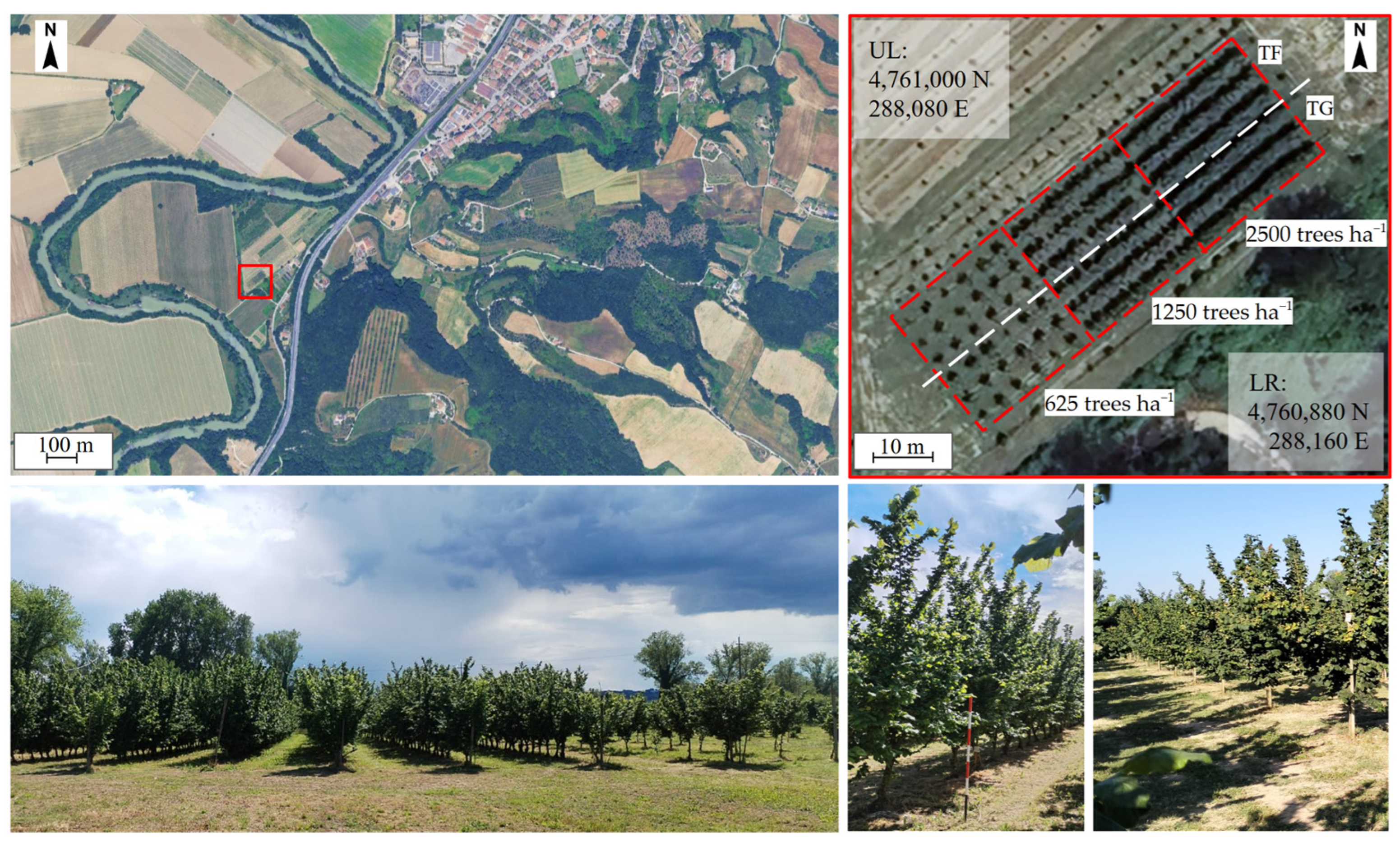
The research was carried out in an experimental orchard managed by the Department of Agricultural, Food, and Environmental Sciences of the University of Perugia, located in central Italy (4760920N, 288120E EPSG:7792-RDN2008/UTM Zone 33N), at 161 m a.s.l. (orthometric height) (Figure 1), during the growing seasons 2021–2024.

The orchard features a split-plot design with three planting densities as main plots:

-

625 trees ha⁻¹ (4 × 4 m spacing);

-

1250 trees ha⁻¹ (4 × 2 m spacing);

-

2500 trees ha⁻¹ (4 × 1 m spacing, experimental treatment).

The 2500 trees ha⁻¹ density was excluded from analyses for two scientifically justified reasons: (1) At tree age 7 (planted 2017), this density causes excessive inter-tree shading (>80% row occlusion, measured via hemispherical photography), reducing net canopy photosynthesis despite high PAR interception (>95%) [22]. (2) It exceeds current commercial recommendations (≤1500 trees ha⁻¹) due to observed yield quality penalties in preliminary trials [23].

All densities include both cultivars. divided into two contiguous but separate planting blocks by variety: Rows 1–3: Tonda di Giffoni (later TG); Rows 4–6: Tonda Francescana^® (later TF) (Figure 1). In each planting block, there are three planting densities from north to south, starting from the densest (2500 trees ha⁻¹) to the least dense (625 trees ha⁻¹). All trees are grafted on Corylus colurna L. non-suckering rootstock and trained as single trunks. Analyses focused exclusively on TF due to: (1) its higher commercial relevance and yield [9]; and the (2) complete UAV coverage availability across all plots. No significant cultivar × density interactions were detected (ANOVA, F = 1.23, p = 0.31; Table S1), justifying cultivar-specific reporting.

The orchard was equipped with a subsurface drip irrigation (SDI) system configured with two lines of Neptune PC AS dripline (pressure-compensating and anti-siphon) (50 cm emitter spacing, 2.4 L/hour flow rate), buried at a depth of 30 cm. Moreover, n. 2 soil moisture sensors (SM100) were installed at depths of 30 cm and 50 cm to monitor soil water content during the growing season.

Meteorological data were monitored by a Spectrum (Thayer Court, Aurora) WatchDog 2000 Series weather station located within the experimental site.

For the growing season 2024, irrigation was applied from 2 July 2024 to 19 August 2024, with a total water volume of 210 m³. Irrigation was managed with a constant dose (or time) each day, except when precipitation occurred.

2.2. UAV Surveys

Multispectral and thermal UAV surveys were conducted on 18 July 2023 and 8 July 2024 at solar noon (±30 min) under clear-sky conditions (Table S2).

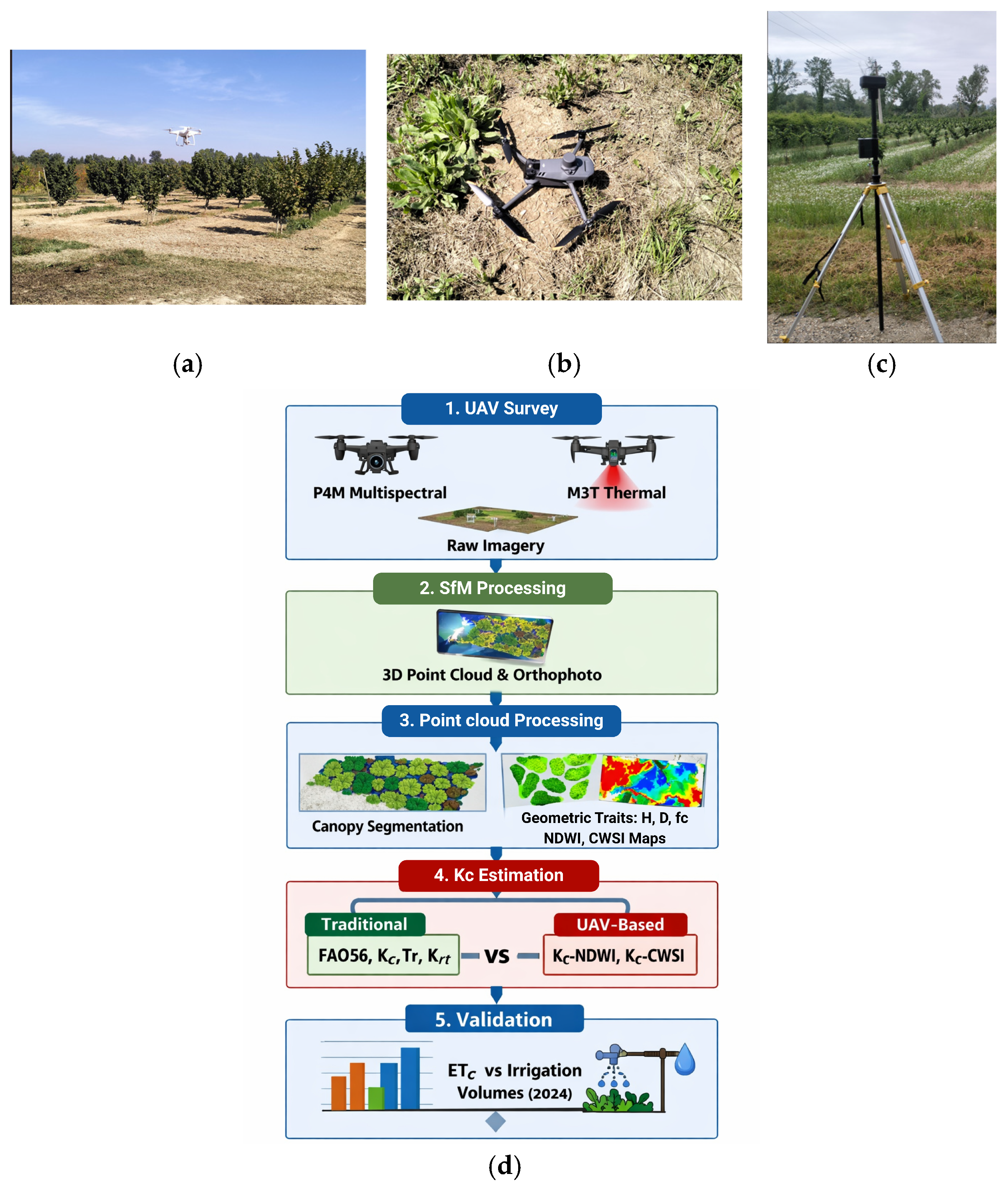
Multispectral surveys were performed using a DJI (Shenzhen, China) Phantom 4 Multispectral P4M (P4M [24], Figure 2a), flying at 10 m altitude with 75% forward and side overlap and a speed of 1.5–2 m s⁻¹, resulting in a ground sample distance (GSD) of approximately 1.5 cm pixel⁻¹. The green (560 ± 16 nm) and near-infrared (840 ± 26 nm) bands were used to compute the Normalized Difference Water Index (NDWI). A spectral sunlight sensor enabled real-time irradiance correction during image acquisition.

Thermal surveys were conducted using a DJI (Shenzhen, China) Mavic 3T (M3T [25]; Figure 2b), flying at 12 m altitude with 75% frontal and lateral overlap and a speed of 1.5–2 m s⁻¹. The thermal sensor provides a spatial resolution of 640 × 512 pixels and 8-bit radiometric data. Thermal image pre-processing was performed using the DJI (Shenzhen, China) Thermal Decoder (SDK-based), which converts raw digital numbers (DN) into temperature-calibrated TIFF images [26].

Both UAV platforms were operated using RTK positioning with a D-RTK 2 mobile station (Figure 2c), supporting GPS, BeiDou, GLONASS, and Galileo constellations to achieve centimeter-level georeferencing accuracy. Flight missions were planned using DJI (Shenzhen, China) GS Pro (iPad).

The resulting multispectral orthophotos were used to derive canopy traits and NDWI, while thermal orthophotos were used to compute the Crop Water Stress Index (CWSI) (Section 2.3). Figure 2d summarizes the overall methodological workflow, including UAV data acquisition, data processing, and the dual estimation of crop coefficients (traditional vs. UAV-based), followed by a consistency check against the irrigation volumes recorded in 2024.

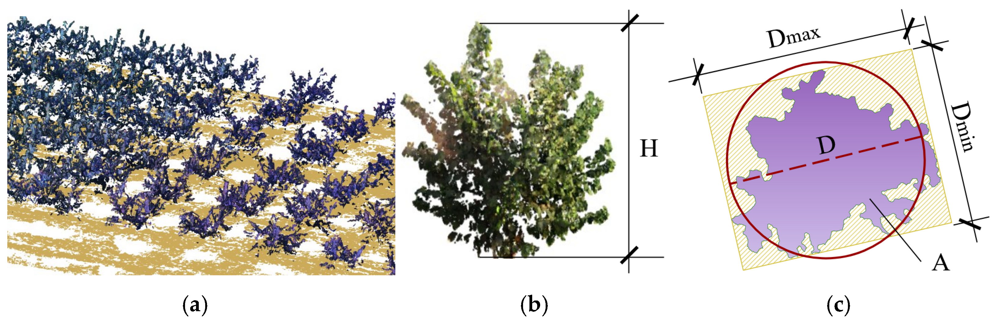
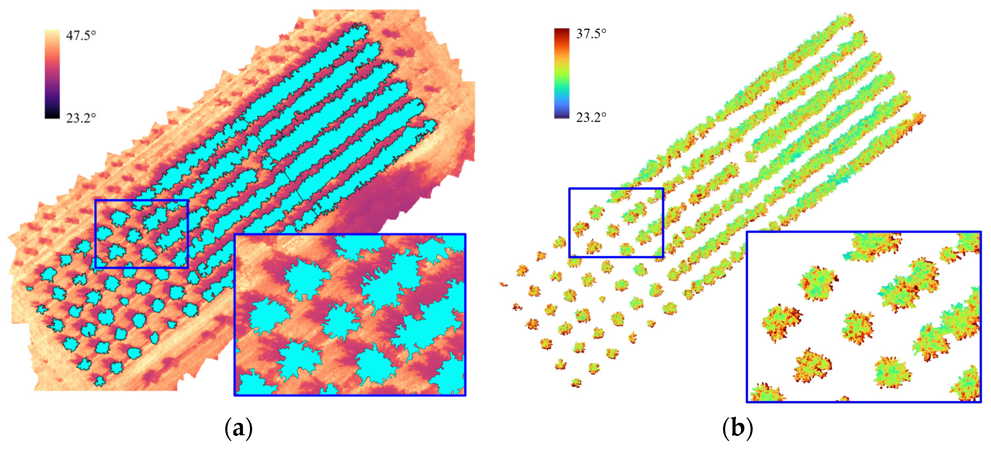
In this study, images acquired by the multispectral sensor were used to extract tree geometrical features, such as canopy mean diameter and height, and to generate NDWI map; thermal sensor data were employed to produce thermal maps, estimate canopy temperature and generate CWSI maps.

2.3. Post-Processing UAV Multispectral and Thermal Data

2.3.1. Point Cloud Reconstruction

Using Agisoft Metashape Professional (v. 1.7.5), images acquired with a multispectral UAV were processed to generate both a point cloud (Figure 3a) and a multispectral orthophoto (Figure 4a) of the orchard. All processing of the point cloud for the derivation of tree geometrical characteristics was performed using Cyclone 3DR software (v. 2024.0). The point cloud was segmented into two subsets: one representing the canopy and the other representing the ground (Figure 3a). From the canopy point cloud, the geometrical features of individual trees were extracted and analyzed for two different tree densities (625 and 1250 trees ha⁻¹), as detailed below:

• Canopy height (H), calculated as the difference between the maximum and minimum elevation values of the canopy point cloud (Figure 3b);
• Canopy area (A), determined by measuring the area of the projected canopy point cloud onto a horizontal plane (Figure 3c);
• Mean canopy diameter (D), obtained as the average of D_min and D_max, the minimum and maximum planimetric dimensions, respectively, of a bounding box around the canopy projection, calculated using a GIS environment (Figure 3c).

A similar procedure was applied to the thermal and RGB images acquired by the DJI Mavic 3T drone. Prior to processing with a Structure-from-Motion (SfM) approach, the thermal images were pre-processed using the DJI (Shenzhen, China) Thermal Decoder tool, based on the DJI (Shenzhen, China) Thermal SDK [26]. This correction was necessary to generate TIFF images in which the digital numbers represent actual temperature values rather than grayscale intensity. The corrected thermal TIFF images were then processed in Agisoft Metashape in a dedicated project to generate a thermal orthophoto (Figure 4b). A separate project was created using the RGB images to generate the point cloud, which, as with the multispectral dataset, was segmented to separate the canopy from the ground, enabling the extraction of the canopy-covered area.

2.3.2. Estimation of Canopy Surface Temperatures from Thermal Images

To determine accurate canopy surface temperatures, the thermal map was first filtered using polygons representing the canopy areas (Figure 5a) to exclude pixels corresponding to the ground, thereby obtaining a thermal map of the canopy surfaces only (Figure 5b). This operation was performed in QGIS and applied to both the 2023 and 2024 surveys. For each canopy area, the mean, minimum, and maximum temperature values were calculated. Additionally, the 10th and 90th percentiles were considered, as some ground pixels may still be present within the canopy polygons.

2.4. Estimation of Crop Coefficients Using Traditional Methods

In this study, the estimation of crop coefficients was done using literature values or applying methods valuable for hazelnut or other fruit crops, as follows:

• The literature values of the single and basal crop coefficients for temperate climate fruit trees, as assessed by López-Urrea et al. [12];
• The method proposed by Vinci et al. [27] under the hypothesis that the evaporative component of the crop evapotranspiration can be negligible and the crop coefficient can be assimilated to the transpiration coefficient (k_c,Tr);
• The procedure described by Fereres et al. [28], where the crop coefficient depends on canopy ground cover.

As assessed by López-Urrea et al. [12], studies referring to hazelnut (Corylus avellana L.) [27,29,30,31,32,33] reported a range of k_c/k_cb values based on the fraction of ground cover fc, the height h, and the training system.

As assessed by [27], the transpiration coefficient (k_c,Tr) tested on hazelnut for both densities, 625 tree/ha and 1250 tree/ha, could be evaluated as follows:

$$k_{c,Tr}=(Q_d·F_1)·F_2$$

(1)

$$Q_d=1-e^{-K_{ext}·V_u}$$

(2)

$$K_{ext}=0.385+0.0047·d_p+12.693-0.909·DAF$$

(3)

$$DAF=1.79+2.83\cdot V_u$$

(4)

$$V_u=V_0·{\displaystyle \frac{d_p}{\mathrm{10,000}}}$$

(5)

$$V_0={\displaystyle \frac{1}{6}}·\pi ·D^2·H$$

(6)

where Q_d is the radiation intercepted by the tree (fraction); F₁ depends on tree density, i.e., F₁ = 0.66 for tree densities >250 trees/ha; F₂ is the monthly tabulated coefficient = 1.25 for June and July; e = 2.718; K_ext is the radiation extinction coefficient; d_p is the tree density (trees/ha); DAF is the leaf area density; V_u is the canopy volume per unit ground surface (m³/m²); V₀ is the canopy volume (m³/tree); D is the canopy’s average diameter (m); and H is the canopy height (m).

The approach by [27] assumes that the soil evaporation component of ET_c is negligible in these micro-irrigated orchards, so that k_c can be assimilated to a transpiration coefficient k_c,Tr. This assumption is reasonable for subsurface drip, where the wetted soil surface is minimal, but may not hold under different irrigation layouts or soil conditions.

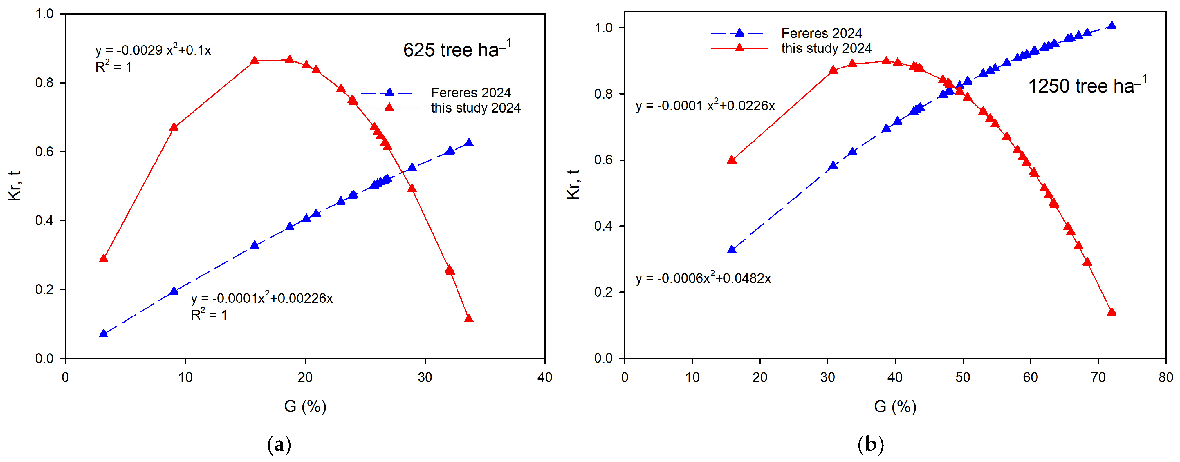
The procedure described by [28] suggests defining a reduction coefficient k_r,t of the crop coefficient k_c to account for a sparsely planted orchard (such as young orchards). Thus, k_r,t is an empirical coefficient of an orchard with incomplete cover relative to a mature orchard. The original k_r,t relationship was developed for young almond orchards; here it is recalibrated using UAV-derived ground cover data to obtain hazelnut-specific coefficients. As suggested by [34], the k_r,t coefficient is related to the horizontal projection of tree shade (ground cover). The relationship between percent ground cover (G%) and k_r,t for almond trees was [28]:

$$k_{r,t}=a·G^2+b·G$$

(7)

with a = −0.00012 and b = 0.0226.

Almond (Prunus dulcis) [35] and hazelnut (Corylus avellana) [9,36] share deciduous canopy architecture, central-leader training systems, comparable leaf area index (LAI 2.5–4.0), and subsurface drip irrigation, which justifies the initial application of almond coefficients as a baseline prior to hazelnut-specific recalibration.

Two-step approach:

• Test almond coefficients [Equation (7)];
• Recalibrate for hazelnut using UAV-derived ground cover (G, 2021–2023) via Equation (17) to obtain hazelnut-specific coefficients [Equations (18) and (19)].

Canopy diameter (D) and height (H) extracted from multispectral point clouds (Section 2.3.1) enabled ground cover (G) estimation for recalibration.

2.5. Estimation of Crop Coefficients Using Vegetation Indices (VIs) from UAV Surveys

Choudhury et al. [37] explored the theoretical basis for using Vegetation Indices (VIs) to replace k_c-FAO. Using wheat as a model crop, they showed the following:

$${Tr}_c={\left({VI}^{\ast }\right)}^{\eta }$$

(8)

where Tr_c is a plant transpiration coefficient (by analogy with k_c) and VI* is a vegetation index stretched between 0 (representing bare soil) and fully transpiring, unstressed vegetation, using the formula:

$${VI}^{\ast }=1-{\displaystyle \frac{{VI}_{max}-VI}{{VI}_{max}-{VI}_{min}}}$$

(9)

VI_max and VI_min are determined from satellite image statistics for individual scenes [38,39].

The exponent η is determined by the relationship between transpiration and the VI used in Equation (8).

Traditional ground-based approaches for kc estimation (e.g., sap flow sensors, lysimeters, and manual ground cover measurements) face significant limitations in high-density hazelnut orchards:

• Spatial sampling bias: Point measurements miss intra-orchard variability driven by differential canopy development, soil heterogeneity, and microclimate gradients [4].
• Labor and cost: Continuous monitoring with sap flow or lysimeters is impractical at commercial scales.
• Temporal resolution: Ground methods cannot provide frequent, wall-to-wall coverage during rapid canopy growth phases.

UAV-based NDWI overcomes these limitations by providing high-resolution (1.5 cm/pixel), spatially continuous maps of canopy water status and ground cover fraction. The empirical VI*-kc relationships (Equations (8) and (9)) [37] have been validated across diverse crops, with power–law exponents (η ≈ 0.3) consistent with our findings, confirming their physical basis linking spectral reflectance to transpiring leaf area.

As assessed above, in this paper the Normalized Difference Water Index (NDWI) and the Crop Water Stress Index (CWSI) were selected as indices relevant to crop water status and used for the estimation of the crop coefficient.

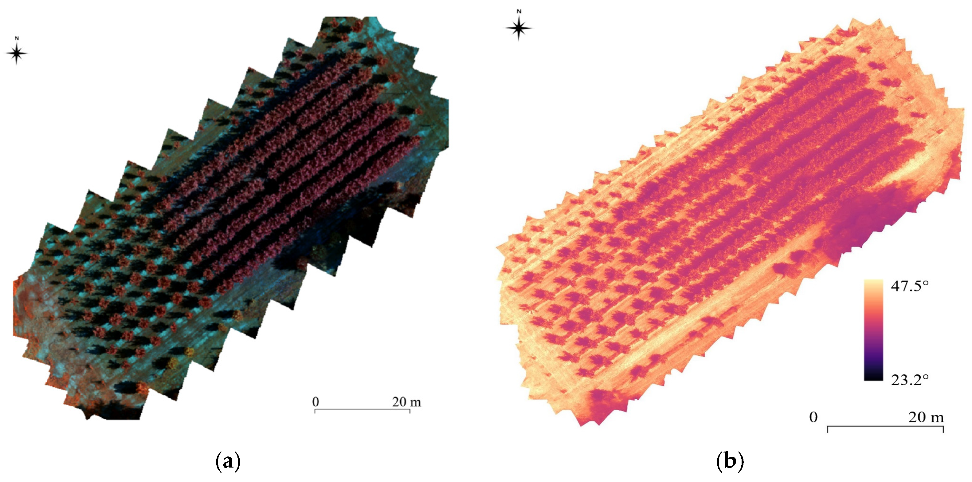
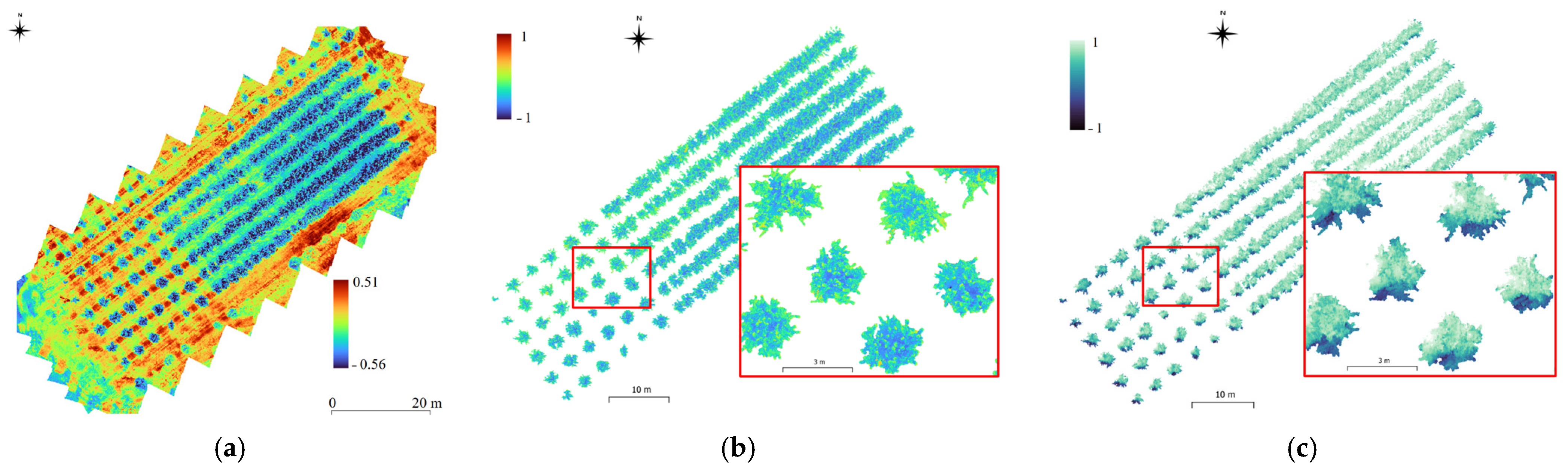
The NDWI map of the entire study area (Figure 6a) was derived from the multispectral orthophoto using Equation (10). The NDWI was subsequently restricted to canopy areas by masking the raster with canopy polygons obtained from the ground projection of the canopy point clouds (Figure 6b). The CWSI was then calculated according to Equation (12) from the thermal map previously masked to canopy areas (Figure 6c). All raster-based calculations were performed in QGIS software (v. 3.34.10).

The Normalized Difference Water Index (NDWI) formulation used in this paper is [38]:

$$NDWI={\displaystyle \frac{Green-NIR}{Green+NIR}}$$

(10)

where Green and NIR are the green and near-infrared bands respectively.

In a GIS environment, the orthophoto derived from corrected thermic images, was used to obtain the thermal map with the formula:

$$T_{meas}={\displaystyle \frac{G_v·(T_{max}-T_{min})}{N_{grey}}}+T_{min}$$

(11)

where T_meas = the temperature registered in the pixel; G_v = the digital number reported in the thermal orthophoto; T_max = the maximum temperature; T_min = the minimum temperature; and N_grey = the total number of values that the pixel can assume, in this case 8-bit, corresponding to 2⁸ = 256 values.

Thermal remote sensing complements spectral indices by monitoring canopy temperature (T_c) and deriving the Crop Water Stress Index (CWSI), originally formulated from the relationship between canopy–air temperature difference and vapor pressure deficit. In its empirical and theoretical versions, CWSI has been widely used as an indicator of crop water status and for irrigation management in different crops [39,40]. Simplified CWSI formulations based on wet and dry reference surfaces have been proposed to avoid the explicit derivation of non-water-stressed baselines under variable environmental conditions [41,42,43].

In this study, canopy temperatures obtained from the thermal camera were used to compute a simplified CWSI, obtained by considering the highest canopy temperature recorded in the image as the dry pixel and the lowest canopy temperature as the wet pixel [20]. Specifically, the following formula was applied [44]:

$$CWSI={\displaystyle \frac{\left(T_c-T_a\right)-(T_{cl}-T_a)}{\left(T_{cu}-T_a\right)-(T_{cl}-T_a)}}$$

(12)

where T_c = canopy temperature (°C); T_a = air temperature (°C); T_cl = temperature of a non-stressed canopy (°C); and T_cu = temperature of a stressed canopy (°C). In practice, to reduce the influence of residual mixed pixels, T_cu and T_cl were derived from the 90th and 10th percentiles of the canopy temperature distribution within each image, respectively.

As assessed by [42] on almonds, canopy temperature and CWSI exhibit substantial intra-crown variability driven by structural heterogeneity and local water status [40,41]. Similar analyses using high-resolution thermal imagery have shown that CWSI variability within the canopy is closely related to stomatal conductance and transpiration patterns, and that robust estimates benefit from focusing on the coldest, purest vegetation pixels [43]. At the individual tree level, differences in liquid-phase resistance to flow between the trunk base and the various parts of the top of the canopy determine variations in water supply that can influence stomatal conductance and T_c. Variability in current and previous radiation exposure can also generate T_c differences between various parts of the tree crown. Furthermore, changes in leaf angle distribution, leaf area density, and canopy architecture may affect T_c. To reduce these effects, for each tree and planting density, the median Tc value, as well as the 10th percentile and 90th percentile, were considered to compute CWSI for each tree.

2.6. Validation of Crop Coefficients Estimated by Traditional vs. Vegetation Indices

The daily crop evapotranspiration ET_c,i, under standard conditions, can be estimated using the k_c-ET₀ approach [45], i.e., as the product between the reference crop evapotranspiration ET₀ and the crop coefficient k_c:

$${ET}_{c,i}=k_c·{ET}_0$$

(13)

The daily series of reference evapotranspiration, ET₀ (mm/day), for the 2024 growing season, were calculated using the FAO Penman–Monteith equation [10]:

$${ET}_0={\displaystyle \frac{0.408∆\left(R_n-G\right)+\gamma \frac{900}{T+273}{u}_2(e_s-e_a)}{∆+\gamma (1+0.34u_2)}}$$

(14)

where R_n is the net radiation at the crop surface (MJ m² day⁻¹), G is the soil heat flux density (MJ m⁻² day⁻¹), T is the mean daily air temperature (°C), u₂ is the wind speed at 2 m height (m/s), e_s is the saturation vapor pressure (kPa), e_a is the actual vapor pressure (kPa), ∆ is the slope vapor pressure curve (kPa °C⁻¹) and γ is the constant psychrometric (kPa °C⁻¹).

Meteorological data collected by the meteorological station were used to evaluate the ET₀.

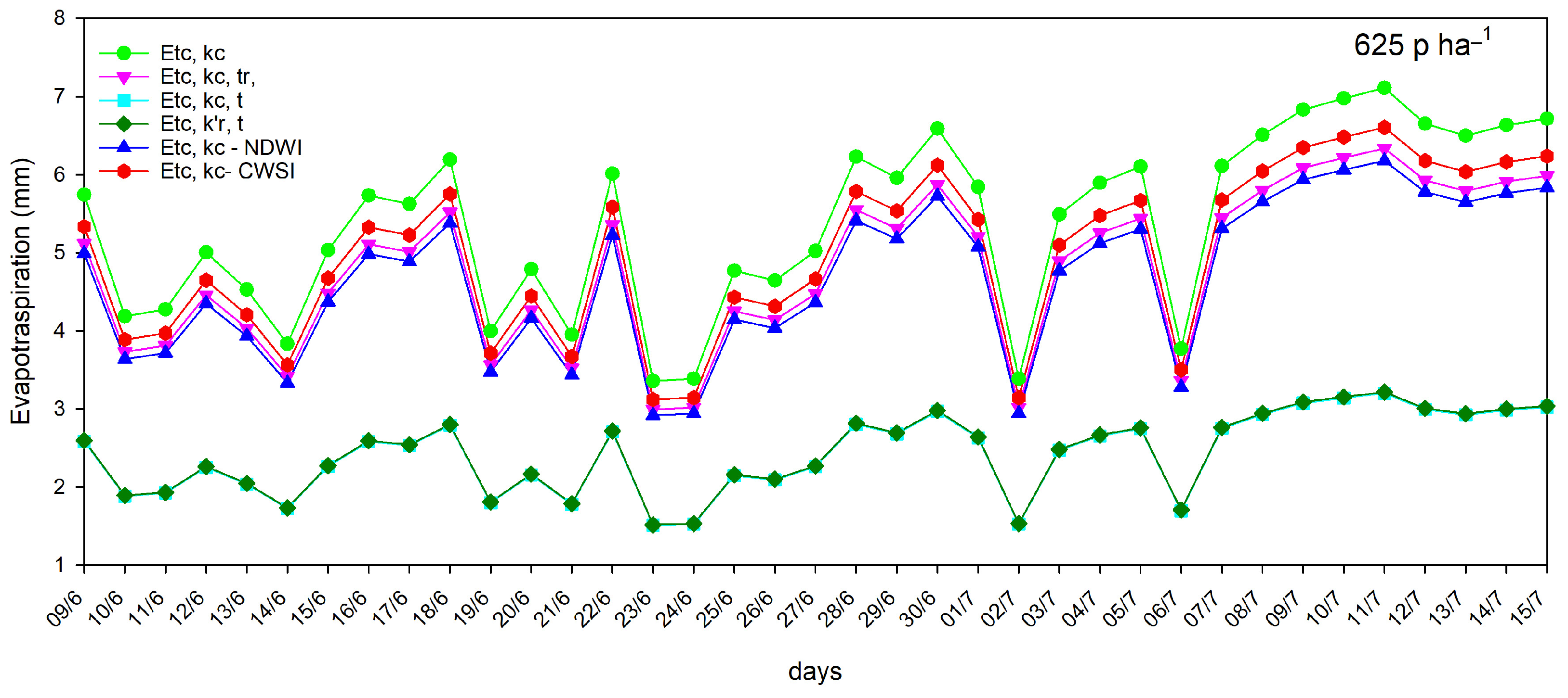
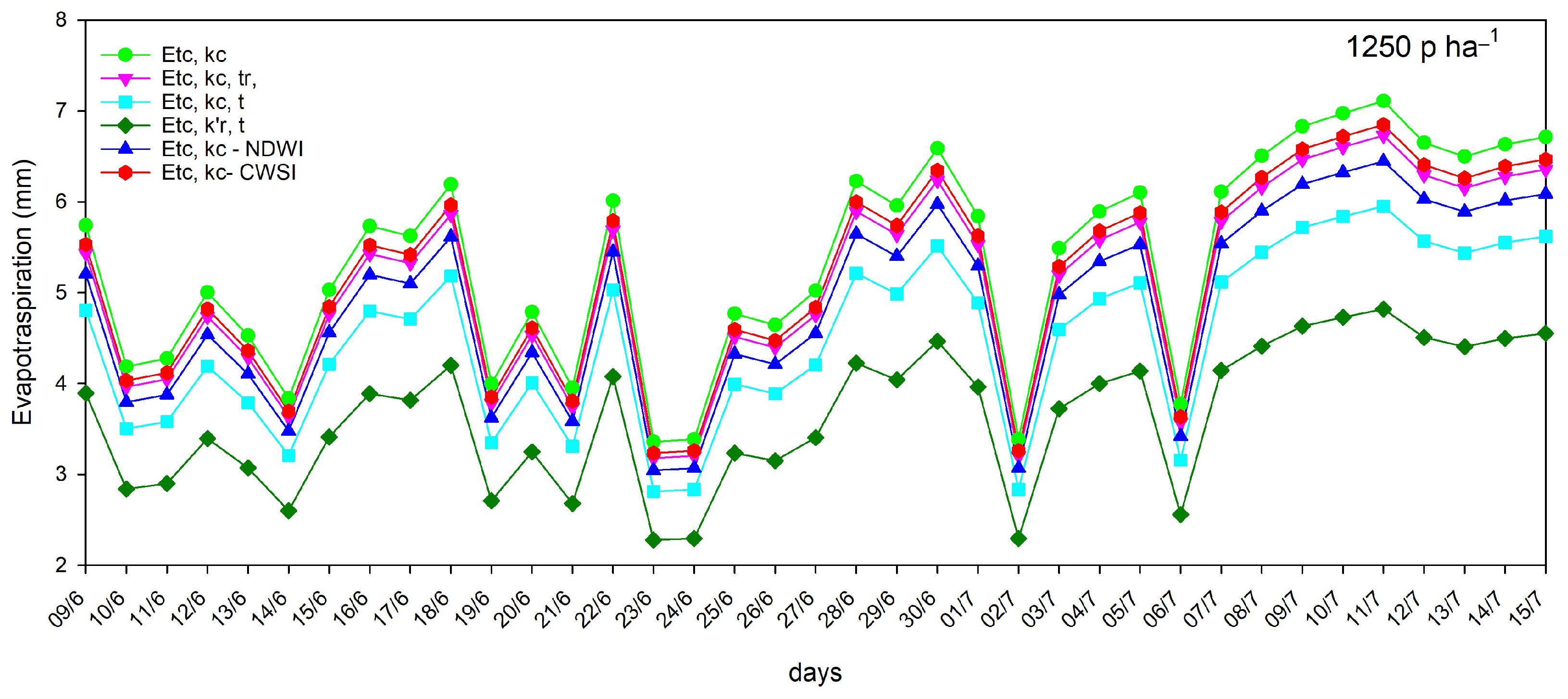
The crop coefficients for the mid-season derived using the traditional methods (k_c, k_c,Tr, k_r,t, $k_{r,t}^{\prime }$) and the Vegetation Indices (k_c-NDWI and k_c-CWSI) were applied to Equation (13) to evaluate the best performance, considering that the term ET₀ depends only on the meteorological characteristics of the 2024growing season.

3. Results

3.1. Estimation of Crop Coefficients Using Traditional Methods

As assessed by [12], considering a medium ground cover (0.55–0.70), the crop coefficients k_c considered in this study was set equal to k_c = 0.9. Applying Equations (1)–(6) described by [27], from Equation (1) the k_c,Tr coefficients for the growing seasons 2023 and 2024 were derived for the plant densities of 625 trees/ha and 1250 trees/ha.

Applying the coefficients a = −0.00012 and b = 0.0226 proposed for almond orchards (Equation (7)) [28], the empirical coefficient k_r,t assessed for the plant density 625 trees/ha and 1250 trees/ha is reported in

Table 1. Values of k_c [12], k_c,Tr [27], k_r,t [28] and $k_{r,t}^{\prime }$(this paper).

		kc	kc,Tr	kr,t [Almond]	${\mathit{k}}_{\mathit{r},\mathit{t}}^{\mathbf{\prime }}$ [Hazelnut, This Study]
2023	625 tree/ha	0.9	0.781	0.327
	1250 tree/ha	0.9	0.824	0.513
2024	625 tree/ha	0.9	0.802	0.450	0.452
	1250 tree/ha	0.9	0.825	0.837	0.678

.

Under the hypothesis that evapotranspiration corresponds to transpiration, Equations (15) and (16) were derived:

$$k_{c,Tr}=k_c·k_{r,t}$$

(15)

$${\displaystyle \frac{k_{c,Tr}}{k_c}}=k_{r,t}$$

(16)

Using Equation (16), an optimization of the relationship between k_r,t and the percent ground area G (%), was made to define the coefficients a and b for grafted hazelnut. The minimum square distance method between the k_r,t simulated using Equation (16) and the relationship with percent ground area from UAV data for the growing seasons 2021, 2022, and 2023 was applied, i.e.,

$$\min \sum {({\displaystyle \frac{k_{c,Tr}}{k_c}}-(a·G^2+b·G))}^2$$

(17)

The coefficients a and b (Figure 7) for hazelnut were:

-

for plant density 625 trees/ha

$$k_{r,t}^{\prime }=a^{\prime }·G^2+b^{\prime }·G=-0.00287·G^2+0.100·G$$

(18)

-

for plant density 1250 trees/ha

$$k_{r,t}^{\prime }=a^{\prime }·G^2+b^{\prime }·G=-0.00064·G^2+0.048·G$$

(19)

3.2. Estimation of Crop Coefficients Using Vegetation Indices (NDWI and CWSI) from UAV Surveys

As assessed in Section 2.5, for each tree and for each plant density, the statistical values (10th percentile, P10, 90th percentile, P90, and median) were evaluated.

Table 2. Vegetation Indices NDWI and temperature of the canopy T_c (median, 10th percentile, P10, and 90th percentile, P90) obtained from UAV surveys.

Plant Density	NDWI			Tc (°C)
	Median	P10	P90	Median	P10	P90
625 tree/ha (2023)	−0.37	−0.61	−0.12	32.09	28.95	35.83
625 tree/ha (2024)	−0.30	−0.55	−0.05	33.45	28.60	39.57
1250 tree/ha (2023)	−0.42	−0.66	−0.15	30.20	27.26	32.79
1250 tree/ha (2024)	−0.33	−0.58	−0.06	30.20	27.26	33.57

reports the statistical values of NDWI and canopy temperature (T_c, used for the estimation of CWSI). The choice of these parameters instead of the literature maximum, minimum and mean values was due to the consideration that index values were evaluated from maps restricted to canopy polygons that were not fully closed; as a result, gaps within the polygons allowed values from the underlying soil to be included. The points corresponding to the ground represent extreme values (lower NDWI or higher temperature), so the statistical parameters were chosen to guarantee the correct evaluation of the NDWI/CWSI values.

NDWI values are negative, but this is expected under the adopted Green–NIR definition when NIR reflectance largely exceeds green reflectance in dense, well-watered canopies. The data confirmed that the orchard was not under stress conditions but showed that the temperature of the canopy for the density 625 trees/ha is higher than that measured for the density 1250 trees/ha (Table 2).

Using the 2023 growing season data, the least squares method was applied to determinate the coefficient η of Equation (8), and the estimated relationships were as follows:

-

for plant density 625 trees/ha:

$$k_{c-NDWI}={\left({NDWI}^{\ast }\right)}^{0.354}$$

(20)

$$k_{c-CWSI}={\left({CWSI}^{\ast }\right)}^{0.170}$$

(21)

-

for plant density 1250 trees/ha:

$$k_{c-NDWI}={\left({NDWI}^{\ast }\right)}^{0.298}$$

(22)

$$k_{c-CWSI}={\left({CWSI}^{\ast }\right)}^{0.25}$$

(23)

Equations (20)–(23) were applied to the data from the 2024 growing season, and the mean values of $k_{c-NDWI}$ and $k_{c-CWSI}$ obtained are reported in

Table 3. Values of k_c-NDWI and k_c-CWSI derived for the 2024 growing season using relationships (20) and (21) for plant density 625 trees/ha and (22) and (23) for plant density 1250 trees/ha.

		kc-NDWI	kc-CWSI
2024	625 tree/ha	0.782	0.836
	1250 tree/ha	0.816	0.867

.

3.3. Validation of Crop Coefficients Estimated by Traditional vs. Vegetation Indices

For the 2024 growing season, the estimation of the actual crop evapotranspiration was obtained by applying the following equations:

$${ET}_{c,K}=K·{ET}_0$$

(24)

with con K equal to k_c (ET_{c, kc}), k_c,Tr (ET_{c, kc,Tr}), k_c-NDWI (ET_{c, kc-NDWI}), and k_c-CWSI (ET_{c, kc-CWSI}), and

$${ET}_c={ET}_0·K^{\prime }$$

(25)

with con K′ equal to the product of k_c and k_r,t (ET_{c, kr,t}) and k_c and $k_{r,t}^{\prime }$ (ET_{c, k’r,t}).

In this analysis, only the period from 9 June to 15 July was considered, as it corresponds to the hottest period for canopy and nut growth of the cultivar Tonda Francescana [46]. Figure 8 and Figure 9 report the dynamics of evapotranspiration evaluated using the different crop coefficients estimated using traditional methods (k_c, k_c,Tr, k_r,t, k’_r,t) and Vegetation Indices (k_c-NDWI and k_c-CWSI) for planting densities of 625 trees/ha and 1250 trees/ha, respectively.

t-tests were applied pairwise between ET_c series derived from different crop coefficients, as no independent measurement of ET_c (e.g., lysimeter or eddy covariance) was available. The values of ET_c obtained were tested using a t-test (with a significance level of 5%), and in

Table 4. Significant or non-significant differences between the values of evapotranspiration evaluated using the different crop coefficients for the plant density of 625 trees/ha.

	ETc-kc	ETc-kc,Tr	ETc-kr,t	${\mathbf{ET}}_{\mathbf{c}}\text{-}{\mathit{k}}_{\mathit{r},\mathit{t}}^{\mathbf{\prime }}$	ETc-kc-NDWI	ETc-kc-CWSI
ETc-kc	-	s	s	s	s	ns
ETc-kc,Tr		-	s	s	ns	ns
ETc-kr,t			-	ns	s	s
${\mathrm{ET}}_{\mathrm{c}}\text{-}{k}_{r,t}^{\prime }$				-	s	s
ETc-kc-NDWI					-	ns
ETc-kc-CWSI						-

and in

Table 5. Significant or non-significant differences between the values of evapotranspiration evaluated using the different crop coefficients for the plant density of 1250 trees/ha.

	ETc-kc	ETc-kc,Tr	ETc-kr,t	${\mathbf{ET}}_{\mathbf{c}}\text{-}{\mathit{k}}_{\mathit{r},\mathit{t}}^{\mathbf{\prime }}$	ETc-kc-NDWI	ETc-kc-CWSI
ETc-kc	-	ns	s	s	ns	ns
ETc-kc,Tr		-	ns	s	ns	ns
ETc-kr,t			-	s	ns	s
${\mathrm{ET}}_{\mathrm{c}}\text{-}{k}_{r,t}^{\prime }$				-	s	s
ETc-kc-NDWI					-	ns
ETc-kc-CWSI						-

(for 625 trees/ha and 1250 trees/ha, respectively) the values that resulted statistically significant (indicated as “s”) or not (indicated as “ns”) were reported.

The primary consideration of this analysis is that the crop coefficient (k_c) used for calculating crop evapotranspiration (ET_c) does not vary with planting density. Therefore, obtaining different results for densities of 625 plants per hectare and 1250 plants per hectare is important for optimizing water supply and reducing water consumption. This could justify the observation that the results obtained with k_c and k_c,Tr are statistically significant in the case of 625 trees/ha, while they are not in the case of 1250 trees/ha. Similarly, this holds true for the k_c-NDWI index. Conversely, the comparison with the k_c-CWSI index did not reveal significant differences for either density. For k_r,t and $k_{r,t}^{\prime }$, the proposed relationship for their determination appears to be a better fit for lower densities. The results obtained for k_c-NDWI and k_c-CWSI values estimated using the two Vegetation Indices show agreement for both densities. This is an interesting result because, being calculated with two UAVs equipped with different sensors, it suggests that their applicability can be adapted to various situations and contexts.

For the hazelnut, from the irrigation point of view, the period of higher water demand corresponds to the growth period (June–15 July); thus, to evaluate the water requirements for both densities (625 trees/ha and 1250 trees/ha), the evapotranspiration during this period was summed (

Table 6. Sum of the water requirements during the period (9 June–15 July) for the plant densities of 625 trees/ha and 1250 trees/ha.

(mm)	ETc-kc	ETc-kc,Tr	ETc-kr,t	${\mathbf{ET}}_{\mathbf{c}}\text{-}{\mathit{k}}_{\mathit{r},\mathit{t}}^{\mathbf{\prime }}$	ETc-kc-NDWI	ETc-kc-CWSI
625 tree/ha	199.359	177.651	89.711	90.110	173.221	185.182
1250 tree/ha	199.359	188.726	166.863	135.165	180.752	192.049

).

3.4. Consistency Check of ET_c Estimates Against 2024 Irrigation Volumes, Testing Transferability to Tonda di Giffoni Cultivar

In this paper, new relationships between the crop coefficient $k_{r,t}^{\prime }$ and the percent ground area G (%) were derived for the Tonda Francescana cultivar (Equations (18) and (19)). Thus, to validate Equations (18) and (19), the data on the percent ground area G (%) of Tonda di Giffoni surveyed using a multispectral UAV on 8 July 2024 were used. The $k_{r,t}^{\prime }$ obtained was 0.67 for 625 trees/ha and 0.75 for 1250 trees/ha and the corresponding ET_c-$k_{r,t}^{\prime }$ (9 June–15 July) was 133.57 mm for 625 trees/ha and 149.52 mm for 1250 trees/ha (

Table 7. Summary of crop coefficients and relative evapotranspiration estimated for the period (9 June–15 July) for the plant densities of 625 trees/ha and 1250 trees/ha.

		${\mathit{k}}_{\mathit{r},\mathit{t}}^{\mathbf{\prime }}$	${\mathbf{ET}}_{\mathbf{c}}\text{-}{\mathit{k}}_{\mathit{r},\mathit{t}}^{\mathbf{\prime }}$
2024	625 tree/ha	0.67	133.57
	1250 tree/ha	0.75	149.52

).

The orchard, as described above, was irrigated from 2 July to 19 August 2024, and the actual water volume distributed corresponded to 214.42 mm/ha for the density 1250 trees/ha and 118.10 mm/ha for 625 trees/ha. The orchard resulted to be not stressed; thus, the water requirements simulated from evapotranspiration should be similar to the amount of water supplied with irrigation and precipitation. The good agreement between ET_c-kr,t/ET_c-$k_{r,t}^{\prime }$ and the applied irrigation volumes holds for the non-stressed conditions and irrigation management adopted in this study; different deficit-irrigation strategies might modify this correspondence. For this reason, the simulated water requirements using the different crop coefficients for the growing season were compared to the water supplied, and the results are reported in

Table 8. Irrigation water requirements simulated during the period (9 June–15 August) for the plant densities of 625 trees/ha and 1250 trees/ha and distributed.

(mm)	Irrigation	ETc-kc	ETc-kc,Tr	ETc-kr,t	${\mathbf{ET}}_{\mathbf{c}}\text{-}{\mathit{k}}_{\mathit{r},\mathit{t}}^{\mathbf{\prime }}$	ETc-kc-NDWI	ETc-kc-CWSI
625 tree/ha	118.10	341.24	305.04	153.56	154.24	303.48	315.92
1250 tree/ha	214.42	341.24	321.04	285.62	231.36	309.52	325.84

.

The data showed an overestimation of water demand during the growing season by all the methods except ET_c-kr,t and ET_c-$k_{r,t}^{\prime }$. These two simulated values were very similar to the distributed water volume. This result suggests applying the reduction coefficients (k_r,t and $k_{r,t}^{\prime }$) to all other methods.

Conceptually, as defined by Fereres et al. [28], the reduction coefficients (k_r,t and $k_{r,t}^{\prime }$), could be applied to all the different crop coefficients (k_c, k_c,Tr, k_c-NDWI, k_c-CWSI) to evaluate the actual evapotranspiration. Thus, in Table 8 and

Table 9. Irrigation water requirements simulated considering the reduction coefficient k_r,t during the period (9 June–15 August) for the plant densities of 625 trees/ha and 1250 trees/ha.

(mm)	Irrigation	ETc-kc	ETc-kc,Tr	ETc-kr,t	${\mathbf{ET}}_{\mathbf{c}}\text{-}{\mathit{k}}_{\mathit{r},\mathit{t}}^{\mathbf{\prime }}$	ETc-kc-NDWI	ETc-kc-CWSI
625 tree/ha	118.10	219.59 *	137.27	153.56	154.24	136.57	142.16
1250 tree/ha	214.42	219.59 *	268.71	285.62	231.36	259.07	272.72

* k_r,t considered was the mean between the values obtained from the two plant densities.

, the water requirements were evaluated as follows:

$${ET}_{c-K^{\prime }}={ET}_0·R_c·K^{\prime }$$

(26)

With K’ = k_c, k_c,Tr, k_c-NDWI, k_c-CWSI, and R_c = k_r,t and $k_{r,t}^{\prime }$.

The values obtained from the analysis are reported in Table 9 (for k_r,t) and

Table 10. Irrigation water requirements simulated considering the reduction coefficient $k_{r,t}^{\prime }$ during the period (9 June–15 August) for the plant densities of 625 trees/ha and 1250 trees/ha.

(mm)	Irrigation	ETc-kc	ETc-kc,Tr	ETc-kr,t	${\mathbf{ET}}_{\mathbf{c}}\text{-}{\mathit{k}}_{\mathit{r},\mathit{t}}^{\mathbf{\prime }}$	ETc-kc-NDWI	ETc-kc-CWSI
625 tree/ha	118.10	192.46 *	137.88	153.56	154.24	137.17	142.79
1250 tree/ha	214.42	192.46 *	217.66	223.32	231.36	209.85	220.92

* k_r,t considered was the mean between the values obtained from the two plant densities.

(for $k_{r,t}^{\prime }$). As expected, the values obtained show good accordance with the irrigation supplied.

4. Discussion

4.1. Crop Coefficients from Traditional Methods and Ground Cover

The results of this study indicate that the standard single crop coefficient (k_c = 0.9) recommended for hazelnut orchards with medium ground cover (0.55–0.70) [12] systematically overestimates crop evapotranspiration (ETc) relative to the irrigation volumes applied in the 2024 season, particularly at the lower planting density (625 trees ha⁻¹). This finding is consistent with the observation that tabulated Kc values, originally developed for mature and fully covering orchards, may not capture the specific water use patterns of young, high-density hazelnut systems where fractional ground cover still remains incomplete [45,47].

The transpiration-based coefficient (k_c,Tr) proposed by [27], which was developed under the assumption that soil evaporation is negligible in subsurface-drip-irrigated orchards, yielded ET_c estimates closer to the applied irrigation volumes (Table 9). This approach explicitly accounts for canopy volume and planting density through the parameters Q_d, K_ext, and DAF (Equations (1)–(6)), thereby reflecting the actual transpiring leaf area rather than a generalized ground cover-based index. The good performance of k_c,Tr supports the hypothesis that, under micro-irrigation with minimal wetted soil surface, the evaporative component (k_e) of total ET_c can indeed be small, and crop water use is predominantly driven by transpiration [10,11,47]. Specifically, the experimental orchard has a silty-loam soil with good water retention. However, this assumption may not hold in orchards with overhead irrigation or in soils with low water-holding capacity, where evaporation from the soil surface can contribute significantly to total ETc [5,16,48].

The observed kc gradient (625 < 1250 trees ha⁻¹) reflects radiation interception scaling with ground cover fraction (fc = 45% vs. 68%). This matches Fereres et al. [28] almond kr,t ~ G² relationship and transpiration models predicting kc ∝ LAI^0.6–0.8 across deciduous trees [49].

The ground cover reduction factors (k_r,t and k′_r,t) provided better agreement with the irrigation volumes than the standard k_c, especially for the 625 trees ha⁻¹ density (Table 4), which is the common plant density in new orchards in Italy. Considering that the original k_r,t coefficients (a = −0.00012, b = 0.0226) were derived from young almond orchards [28] and applied here as a reference, we recalibrated these coefficients using multi-year UAV-derived ground cover data (2021–2023, [50,51]). This produced hazelnut-specific relationships (Equations (18) and (19)) that better captured the nonlinear dependency of k_c on fractional cover for both planting densities. The obtained coefficients (k′_r,t) showed no statistically significant difference from k_c,Tr (Table 4), confirming that ground cover-based reduction factors can effectively adjust tabulated k_c values to account for both incomplete canopy development in young orchards [45,52] and the most upright canopy of grafted plants, which results in less vegetation cover [49].

These results are in line with recent findings for other high-density fruit tree systems, where crop coefficients increase with canopy height and fractional ground cover, reaching values close to FAO56 references only at full canopy closure [6,7,13,14,15,53]. For hazelnut specifically, ref. [54] reported mid-season k_c values of approximately 0.85–0.95 for mature orchards and plant densities of over 500 trees ha⁻¹ under Mediterranean conditions, which are higher than the k_c,Tr and k′_r,t values obtained in our study (0.78–0.83) for young grafted trees. Similarly, ref. [55] proposed monthly k_c values for hazelnut in Tarragona (Spain) that varied with phenological stage and irrigation method and noted that hazelnut is sensitive to water stress and prefers cooler, more humid conditions [48,56].

4.2. Crop Coefficients Derived from UAV-Based Vegetation Indices

The empirical relationships calibrated between crop coefficients and UAV-derived NDWI and CWSI (Equations (20)–(23)) produced mid-season k_c estimates (0.78–0.87) that were statistically indistinguishable from the transpiration-based k_c,Tr (Table 3), demonstrating the potential of remote sensing indices to replace or complement ground-based measurements in estimating hazelnut water requirements. This finding is consistent with previous studies on vineyards and apple orchards, where spectral Vegetation Indices have been successfully linked to k_c and k_cb through power or exponential functions [5,6,7,13,14,15,16].

NDWI captures structural development (canopy density), while CWSI reflects physiological water status. Their close agreement (Δkc < 0.03) under subsurface drip irrigation confirms the non-stressed baseline conditions, enabling direct kc-CWSI linkage without stress correction factors.

The choice of NDWI as a proxy for k_c was motivated by its sensitivity to canopy water content and vegetation density [17,18]. The negative NDWI values observed in this study (Table 2) are expected when using the Green–NIR formulation in dense, well-watered canopies where NIR reflectance greatly exceeds green reflectance [18,38]. The normalization procedure (Equation (9)) stretches these values between the observed minimum and maximum within each image, producing a dimensionless index (NDWI*) that correlates with fractional ground cover and leaf area [37,57]. The resulting power–law relationships (η = 0.35 for 625 trees ha⁻¹, η = 0.30 for 1250 trees ha⁻¹) are within the range reported for other crops, where exponents typically vary from 0.2 to 0.5 depending on canopy architecture and the specific vegetation index used [5,53].

Similarly, the CWSI-based coefficients (k_c-CWSI) captured the thermal signature of crop water status, with values close to k_c,Tr and slightly higher than k_c-NDWI (Table 3). The simplified CWSI formulation adopted here [20,44], which uses the warmest and coolest canopy pixels as dry and wet references, avoids the need for empirical baselines relating canopy–air temperature differences to vapor pressure deficit [39,58]. This approach is particularly well-suited for UAV thermal imaging, where high spatial resolution allows pure vegetation pixels to be isolated from the soil background and where intra-canopy variability can be substantial [4,43,59].

These findings on grafted hazelnut agree with recent work by [60], who developed a CWSI model for hazelnuts in Oregon using low-cost infrared thermometers and validated it against stem water potential and leaf conductance. They reported that CWSI values below 0.2 corresponded to stem water potentials above −6 bar and leaf conductance rates of 0.2–0.4 mol m⁻² s⁻¹, indicating low plant stress. In this study, the canopy temperature data (Table 2) and the resulting CWSI maps (Figure 6b) confirmed that the orchard was not under water stress during the UAV surveys, consistent with the irrigation management applied. The higher canopy temperatures observed for the 625 trees ha⁻¹ density compared to 1250 trees ha⁻¹ (Table 2) likely reflect differences in canopy density and shading, with more spaced trees experiencing greater radiative heating [42], as also reported by [60].

Moreover, the use of percentiles P10, P90, and median rather than absolute minimum and maximum temperatures to characterize canopy thermal variability was motivated by the presence of residual mixed pixels at canopy edges, where incomplete polygon closure can introduce outliers from the soil background [40,59]. Refs. [4,42] showed that this statistical filtering approach may improve the robustness of CWSI estimates in heterogeneous tree canopies.

4.3. Comparison with Other Fruit Crops

The derived kc-NDWI (0.78–0.82) and kc-CWSI (0.84–0.87) values for hazelnut demonstrate an excellent comparability with published coefficients for deciduous fruit trees (

Table 11. Comparison of mid-season kc values: this study vs. literature (fruit crops).

Crop	Density (Trees ha−1)	Method	kc Mid-Season	Reference
Hazelnut	625	kc-NDWI	0.78	This study
Hazelnut	1250	kc-NDWI	0.82	This study
Hazelnut	625	kc-CWSI	0.84	This study
Hazelnut	1250	kc-CWSI	0.87	This study
Almond	500	NDVI-based	1.05–0.9	Bellvert [61]
Pistachio	500	NDVI-based	0.89–0.80	Bellvert [61]
Citrus	400	NDVI	0.55	Ippolito [62]

) at similar planting densities and canopy development stages:

• Almond orchards (<500 trees ha⁻¹): Bellvert et al. [61] reported NDVI-based kc = 1.05–0.90, higher than our 625 trees ha⁻¹ due to almond’s larger mature canopy size (LAI 3.5 vs. hazelnut LAI 2.8);
• Pistachio orchards (<500 trees ha⁻¹): Bellvert et al. [61] reported NDVI-based kc = 0.89–0.80, similar to our 625 trees ha⁻¹ and 1250 trees ha⁻¹ values.
• Citrus orchards (400 trees ha⁻¹): Ippolito et al. [62] found kc-NDVI = 0.55 for lower canopy cover (fc < 48%), lower than our 1250 trees ha⁻¹ hazelnut (fc = 65%), consistent with ground cover scaling.

These cross-crop comparisons validate the UAV-NDWI/CWSI methodology and demonstrate that hazelnut coefficients follow established patterns observed in almond, peach, and olive systems, enhancing confidence in operational transferability. Therefore, as assessed by [63], CWSI seems to be more sensitive to transient changes in orchard water use and stress, whereas NDVI values are generally more stable.

4.4. Consistency Check of ETc Estimates Against 2024 Irrigation Volumes: Testing Transferability to Tonda di Giffoni Cultivar

The consistency check of the different k_c approaches against the applied irrigation volumes (Figure 1 and Figure 2; Table 4 and Table 5) represents an indirect assessment of ET_c estimation accuracy, as no direct measurements of actual evapotranspiration (e.g., eddy covariance or weighing lysimeters) were available. The sandy-loam texture + 30cm SDI depth suggest 15–20% losses, explaining why irrigation < ET_c, while soil moisture remained adequate (θ > 0.20 m³/m³). Recent studies on hazelnut orchards have employed eddy covariance systems to quantify ET_a and k_c at high temporal resolution. Ref. [64] reported seasonal k_c values for a drip-irrigated ‘Tonda di Giffoni’ orchard in Chile (Mediterranean semi-arid climate) using three growing seasons of eddy covariance data, providing the first detailed quantification of ET_a dynamics and surface energy balance components for this cultivar [65]. Their k_c estimates showed substantial intra- and inter-seasonal variability driven by canopy development and climatic conditions, with mid-season values comparable to those obtained in our study using UAV-based indices.

The good agreement between ET_c estimated from ground cover-adjusted coefficients (k_r,t, k′_r,t) and the irrigation volumes applied supports the hypothesis that, under non-stressed conditions and adequate subsurface drip management, the applied water approximates actual crop water use [35]. However, this correspondence may not hold under deficit-irrigation strategies or in the presence of significant deep percolation or runoff, which would decouple applied volumes from ETc [16,47,48].

The transferability of the calibrated NDWI and CWSI relationships to the cultivar Tonda di Giffoni (objective 3) was successfully tested in this study, suggesting that the UAV-based approach could be adapted with minor recalibration when applied to cultivars with similar traits [49] and similar training systems [66]. Future work should validate these relationships across multiple cultivars, sites, training systems and irrigation regimes to assess their generalizability [5].

5. Implications for Irrigation Scheduling in Hazelnut Orchards

The combination of traditional methods (ground cover reduction factors and transpiration-based coefficients) with UAV-derived spectral and thermal information offers a flexible framework for estimating crop coefficients in hazelnut orchards. The main advantages of the UAV approach are as follows:

• Spatial resolution: UAV imaging captures intra-orchard variability in canopy development and water status, which is not reflected in plot-averaged ground measurements [4,5].
• Temporal flexibility: Surveys can be scheduled to match critical phenological stages (e.g., mid-season peak LAI, pre-harvest water stress) without the need for continuous sensor deployment [53].
• Scalability: Once calibrated, the empirical relationships (Equations (20)–(23)) can be applied to larger areas using satellite data (Landsat, Sentinel-2) for operational irrigation management [6,65].

The proposed hazelnut ground cover coefficients (k′_r,t) represent a simple and practical tool for adjusting tabulated k_c values in grafted orchards, requiring only UAV-derived ground cover estimates or manual measurements. This approach is particularly relevant for growers transitioning to high-density systems (625–1250 trees ha⁻¹), such as those increasingly adopted in Chile [23,67,68], where standard FAO56 coefficients may lead to over-irrigation and reduced water use efficiency [45,52].

For operational applications, we recommend the following decision hierarchy:

• If UAV data are available: use kc-NDWI or kc-CWSI (Equations (20)–(23)) for site- and season-specific estimates;
• If only ground cover is known: apply k′_r,t (Equations (18) and (19)) to adjust the standard k_c = 0.9;
• If neither is available: use k_c,Tr (Equation (1)) with measured or estimated canopy dimensions (D, H), which performed well in our consistency check.

6. Conclusions

This study demonstrates that combining traditional crop coefficient estimation methods with UAV-derived spectral and thermal indices can significantly improve the accuracy of evapotranspiration estimates in hazelnut orchards. The main findings are as follows:

• The standard FAO56 crop coefficient (k_c = 0.9) overestimated ET_c relative to applied irrigation volumes, particularly at lower planting density (625 trees ha⁻¹), highlighting the need for site-specific adjustments in other conditions (i.e., training systems).
• Ground cover reduction factors (k_r,t, k′_r,t) calibrated from multi-year UAV data provided a simple and effective method to adjust tabulated Kc values, yielding estimates comparable to transpiration-based coefficients (k_c,Tr).
• UAV-derived NDWI and CWSI were successfully linked to crop coefficients through empirical power–law relationships, producing mid-season k_c values statistically equivalent to k_c,Tr and offering a spatially explicit alternative to plot-averaged measurements.
• The proposed relationships (Equations (16)–(23)) are ready for operational use in similar hazelnut systems and can be extended to satellite platforms for larger-scale irrigation management.

These results support the adoption of remote sensing tools in precision irrigation of high-density hazelnut orchards, contributing to improved water use efficiency and sustainable intensification of nut production in water-limited Mediterranean environments.

Future research should also explore the integration of UAV-based k_c estimates with soil moisture sensors and weather forecasts to develop real-time irrigation scheduling tools for hazelnut growers, similar to recent advances in precision irrigation for other tree crops [6,48,58].

The primary methodological limitation is the lack of direct measurements of actual crop evapotranspiration (ET_a) using reference methods such as lysimeters, sap flow sensors, or eddy covariance systems. Without ground-truth ET_a data, the agreement between modeled ET_c and irrigation volumes constitutes a management consistency check rather than definitive model validation. While UAV-NDWI/CWSI coefficients produced ET_c estimates within ±15% of applied irrigation, this cannot confirm absolute accuracy in the absence of independent ET_a data.

The NDWI/CWSI-k_c relationships were calibrated using 2023 data for the Tonda Francescana^® cultivar and tested with 2024 same-site data. The spatial transferability was untested (single orchard) in this study; thus, multi-site/multi-cultivar validation is required for operational deployment.