Estimation of Canopy Traits and Yield in Maize–Soybean Intercropping Systems Using UAV Multispectral Imagery and Machine Learning

Abstract

Strip intercropping of maize and soybean is a key practice for improving land productivity and ensuring food and oil security in the hilly regions of the Loess Plateau. However, complex interspecific interactions generate highly heterogeneous canopy structures, making it difficult for traditional linear models to capture yield variability within mixed pixels. Based on a single-season (2025) field experiment, this study developed a UAV multispectral imagery-based yield estimation framework integrating multiple machine-learning algorithms. Shapley additive explanations (SHAP) and partial dependence plots (PDP) were used to interpret the spectral–yield relationships under different spatial configurations. The predictive performance of linear regression and eight nonlinear algorithms was compared using 20 spectral features. Ensemble learning outperformed linear approaches in all intercropping scenarios. In the maize–soybean 3:2 pattern, the GBDT model delivered the highest accuracy (R² = 0.849; NRMSE = 9.28%), whereas in the 4:2 pattern with stronger shading stress on soybean, the random forest model showed the greatest robustness (R² = 0.724). Interpretation results indicated that yield in monoculture systems was mainly driven by physiological traits characterized by visible-band indices, while yield in intercropping systems was dominated by structural and stress-response traits represented by near-infrared and soil-adjusted vegetation indices. The generated centimeter-scale yield maps revealed clear strip-like spatial variability driven by interspecific competition. Overall, explainable machine learning combined with UAV multispectral data shows promise for within-season yield estimation in intercropping systems and can support spatially differentiated precision management under the sampled conditions.

1. Introduction

Maize–soybean strip intercropping is one of the most important cropping systems for coping with water scarcity and improving land productivity in the hilly regions of the Loess Plateau in China [1,2]. By arranging tall crops (maize) and short crops (soybean) in a rational spatial configuration, this system exploits niche complementarity in light interception, nutrient uptake, and root distribution, thereby achieving a land equivalent ratio greater than 1 + 1 > 2 [3,4]. However, while increasing total productivity, intercropping simultaneously introduces pronounced within-field spatial heterogeneity. Border-row maize often exhibits yield advantages because it occupies more lateral light and soil resources, whereas soybean adjacent to tall maize rows suffers shading stress and consequent yield reduction [5,6]. Such spatial variability driven by interspecific competition and complementarity makes conventional uniform field management insufficient to match the actual crop requirements, resulting in low water–fertilizer use efficiency and unexploited yield potential [7,8]. Therefore, accurately characterizing the spatial distributions of crop yield within intercropping systems is of great significance for optimizing resource allocation, implementing site-specific variable management, and enhancing the overall benefits of strip intercropping.

However, in practical field management, rapid, accurate, and non-destructive monitoring of yield in intercropping systems remains highly challenging [9,10]. Traditional manual sampling and laboratory analysis can provide reliable ground truth data, but these approaches are destructive, labor-intensive, and costly, with low temporal resolution, making it difficult to continuously monitor crop growth dynamics [11]. In maize–soybean intercropping fields in particular, yield differences between crop strips may vary sharply over only a few meters or even between adjacent rows, resulting in poor spatial representativeness of manual sampling [12]. Moreover, destructive sampling is usually restricted to the maturity stage, preventing the provision of early-warning information during the growing season. Consequently, field management decisions are often made in a reactive manner (“after-the-fact remediation”) rather than through proactive regulation [13]. Limitations in both monitoring technologies and methodologies (e.g., sensor/deployment constraints and sampling/calibration protocols) have constrained precision management in intercropping systems and hindered the full realization of the ecological advantages of strip intercropping in terms of resource-use efficiency. From an ecological perspective, strip intercropping benefits from resource partitioning, whereby component crops reduce direct competition by differentiating resource use across space and time (e.g., complementary light capture and staggered water/nutrient uptake). Without sufficiently resolved monitoring, these fine-scale complementary processes are difficult to diagnose and translate into actionable, targeted management.

Process-based crop growth models such as APSIM (Agricultural Production Systems sIMulator) and DSSAT (Decision Support System for Agrotechnology Transfer) are theoretically capable of simulating crop development and yield formation processes [14,15]. However, these models require precise inputs of soil hydro-physical properties, cultivar-specific genetic parameters, and daily meteorological data, which are difficult to obtain accurately at the field scale and often exhibit strong spatial heterogeneity [16,17]. More importantly, most existing crop models were developed for monocropping systems, and they face substantial limitations in mechanism applicability when dealing with the complex interspecific interactions in intercropping systems, including light competition, nutrient competition, and root–root interactions [18]. Although remote sensing techniques have performed well in assessing crop growth at regional scales, satellite-based observations are constrained by coarse spatial resolution (typically >10 m) and relatively long revisit intervals (from several days to weeks), making them unable to capture fine-scale yield variability at the meter or row scale in strip intercropping fields [19,20]. Therefore, achieving a balance between low cost and high accuracy, and realizing near-real-time, high-resolution yield monitoring for intercropping systems, remains a central challenge in precision agriculture research and practice [21].

In recent years, with the rapid development of lightweight unmanned aerial vehicle (UAV) platforms and multispectral sensor technology, UAV-based remote sensing has shown great potential for crop phenotyping and yield estimation [22,23,24]. Compared with satellite remote sensing, UAVs offer centimeter-level spatial resolution (<10 cm), flexible on-demand flight capability, and relatively low data acquisition costs, enabling detailed characterization of canopy heterogeneity at the field scale [25]. Previous studies have demonstrated significant correlations between vegetation indices derived from UAV multispectral imagery (e.g., NDVI, GNDVI, NDRE) and crop biomass, leaf area index, and final yield, providing a technical basis for non-destructive yield monitoring [26,27]. Meanwhile, the introduction of machine-learning approaches has further enhanced the rapid, timely, and cost-effective information-capturing capability of remote sensing data. Nonlinear algorithms such as random forest (RF), gradient boosting decision trees (GBDT), and extreme gradient boosting (XGBoost) can construct high-dimensional feature spaces and effectively capture the nonlinear relationships between spectral features and crop traits under complex environments [28,29,30]. However, most studies have focused on monocropping systems or simple mixed cropping, and systematic investigations remain scarce regarding maize–soybean strip intercropping systems, which are characterized by highly regular spatial configurations and complex interspecific interactions. In particular, issues such as yield inversion accuracy, optimal algorithm selection, and spectral response mechanisms under UAV–machine-learning frameworks have not yet been comprehensively addressed [31,32].

In addition, traditional machine-learning models are often regarded as “black boxes,” making it difficult to interpret the internal logic of model decisions and the contribution of different features [33]. The lack of interpretability not only limits the credibility of such models in agronomic practice but also hampers a deeper understanding of yield formation mechanisms in intercropping systems. In maize–soybean intercropping in particular, yield variability is jointly regulated by multiple factors, including canopy structural effects (border-row advantage), physiological functions (stay-green characteristics), and stress responses (shade adaptation), and the dominant factors may shift dynamically under different planting configurations (row ratios) [34]. Therefore, evaluating model performance solely on the basis of prediction accuracy is insufficient. It is urgently necessary to incorporate interpretability tools, such as SHAP and partial dependence plots (PDP), to elucidate the agronomic mechanisms underlying the spectral–yield responses under different spatial configurations, thereby providing theoretical support for the agronomic application of machine-learning models.

Against this background, this study focuses on maize–soybean strip intercropping systems and proposes a high-accuracy yield estimation framework that integrates UAV multispectral remote sensing with explainable machine learning. Multi-scenario experiments involving monocropping and different strip-intercropping configurations (3:2 and 4:2) were established to comprehensively evaluate the yield prediction performance of eight algorithms—linear regression, regularized regression, k-nearest neighbors, random forest, gradient boosting decision trees, and XGBoost—under complex planting patterns, and to identify the optimal inversion models for specific “crop–pattern–trait” combinations. Here, 3:2 and 4:2 refer to soybean-to-maize row arrangements within one repeating strip unit (3:2 = three soybean rows plus two maize rows; 4:2 = four soybean rows plus two maize rows). On this basis, SHapley Additive exPlanations (SHAP) were used to quantify the marginal contributions of spectral features to yield prediction, while partial dependence plots (PDP) were employed to analyze the nonlinear response relationships between key features and yield, thereby revealing shifts in yield formation mechanisms driven by planting configuration. Finally, we derive high-resolution yield maps from UAV multispectral imagery to characterize within-field spatial variability and to distinguish two dominant drivers of yield patterns, namely, soil background heterogeneity and interspecific competition. These results provide essential data support for zone-specific precision management in intercropping systems. Overall, this study offers a low-cost and scalable technical pathway for intelligent monitoring of composite cropping systems and provides a scientific basis for optimizing intercropping patterns and precision agronomic decision-making in the hilly regions of the China’s Loess Plateau.

2. Materials and Methods

2.1. Research Area Overview

This study was conducted in Dongpanliang Village (37°06′ N, 111°53′ E), Xiaoyi City, Shanxi Province, China (Figure 1). The village is administratively located in Daxiaobao Town, Xiaoyi City, Lüliang City, Shanxi Province, China. The experimental area is located in the hilly region of the Loess Plateau and is characterized by a typical temperate continental monsoon climate. The region has four distinct seasons, with a mean annual temperature of approximately 13 °C. The long-term mean annual precipitation is 477 mm, with markedly uneven temporal and spatial distribution, and most rainfall occurs during the crop growing season from June to September. The frost-free period is about 170 days, and the available heat resources are sufficient to support one growing season of maize and soybean. The soil in the experimental fields is mainly classified as Haplic Luvisol (locally referred to as cinnamon soil or brown loam), with a deep profile and loam texture, exhibiting good water-holding capacity and aeration. Measurements of the 0–20 cm plow layer indicated that soil organic matter content ranged from 10.27 to 15.30 g·kg⁻¹ (1.027–1.53%), total nitrogen from 0.75 to 0.90 g·kg⁻¹ (0.0745–0.0903%), available phosphorus from 9.3 to 16.5 mg·kg⁻¹, and available potassium from 98 to 131 mg·kg⁻¹. Soil pH ranged from 7.3 to 7.5, indicating neutral to slightly alkaline conditions. Field experiments were continuously conducted from 2023 to 2025 and included maize–soybean strip intercropping systems with 3:2 and 4:2 configurations, as well as monocropping systems. Throughout the experiment, drip irrigation was used to supply supplemental water. Meteorological variables (e.g., air temperature, precipitation, solar radiation, and relative humidity) were measured by an on-site automatic weather station installed within the experimental base and aggregated to the temporal resolution used for modeling. Soil type was determined based on composite soil samples collected from the experimental plots and analyzed following standard laboratory procedures.

2.2. Data Collection and Processing

2.2.1. Experimental Design and Field Management

The maize cultivar used in this study was ‘Qiangsheng 199’ (Zea mays L. cv. Qiangsheng 199), and the soybean cultivar was ‘Xidou 5’ (Glycine max (L.) Merr. cv. Xidou 5). Both cultivars are widely cultivated locally and showed stable establishment and normal growth under the field conditions of this study; therefore, they were selected as representative local cultivars for evaluating UAV-based phenotyping and yield mapping in strip intercropping. To ensure that crop growth was not limited by water deficits in the semi-arid environment, drip irrigation was adopted. Drip lines were laid between crop rows, and irrigation and fertilization were scheduled according to crop water requirements to achieve precise water–fertilizer management. Apart from irrigation treatments, other agronomic practices (e.g., fertilization, irrigation, and pest/weed management) were applied uniformly across treatments to standardize management inputs and control their variability, thereby reducing potential confounding effects on crop phenotypes.

2.2.2. Ground Phenotype Parameter Measurement

To obtain reliable ground-truth data, field measurements were carried out in 2025 during the maize jointing, big-bell, tasseling, grain-filling, and maturity stages, and all ground operations were synchronized with UAV flights. Nondestructive observations were first conducted. Leaf area index (LAI) was measured using an LAI-2200C plant canopy analyzer (LI-COR, Lincoln, NE, USA). To account for inter-row heterogeneity in strip intercropping, a “one-above and four-below” sampling scheme was applied, in which one reading was taken above the canopy and four readings were taken below the canopy at different inter-row positions to ensure measurement representativeness. Meanwhile, SPAD values of functional leaves (the third leaf below the ear) were recorded using a FieldScout CM 1000 portable chlorophyll meter (Spectrum Technologies, Inc., Aurora, IL, USA). SPAD values are dimensionless readings that provide a relative index of leaf chlorophyll content (leaf greenness) and are widely used as a rapid proxy for chlorophyll-related status and, indirectly, crop nitrogen status. This instrument is based on ambient-light reflectance and avoids physical damage associated with contact measurements. For each plot, 5–10 repeated measurements were taken.

After the nondestructive measurements, destructive sampling was immediately conducted to determine aboveground biomass (AGB). Within the sampling area of each plot, three uniformly growing plants were randomly selected and carefully excavated with their roots. The roots were then removed, and the aboveground parts were rinsed with clean water. Plants were separated into different organs (stem, leaf, and sheath) and ears (after tasseling), and each component was individually bagged. The samples were first heated at 105 °C for 30 min to inactivate enzymatic activity and then dried at 80 °C to constant weight in a forced-air oven. The dry mass of each component was weighed and summed to obtain the dry mass per plant, which was subsequently converted to unit-area AGB (g m⁻²) according to plant density. Meanwhile, leaf water content (LWC) was calculated from fresh and dry leaf weights (Equation (1)).

$$\mathrm{L}\mathrm{W}\mathrm{C}={\displaystyle \frac{\mathrm{F}\mathrm{W}-\mathrm{D}\mathrm{W}}{\mathrm{F}\mathrm{W}}}\times 100\%$$

(1)

In Equation (1), LWC denotes canopy leaf water content, FW represents leaf fresh weight, and DW indicates leaf dry weight.

2.2.3. UAV Data Acquisition and Processing

UAV remote-sensing observations were strictly synchronized with ground-based phenotypic measurements in both time and space. A DJI Mavic 3M (Mavic 3 Multispectral) UAV was used as the data acquisition platform. The system is equipped with an RTK module providing centimeter-level positioning accuracy and carries a 20-MP RGB camera together with four 5-MP multispectral cameras. The center wavelengths of the multispectral bands are green (560 nm, bandwidth 16 nm), red (650 nm, 16 nm), red-edge (730 nm, 16 nm), and near-infrared (860 nm, 26 nm). A multispectral irradiance sensor mounted on the top of the UAV continuously recorded incoming solar radiation to compensate for illumination differences among flight times. All flights were performed under clear-sky conditions between 11:00 and 14:00 to ensure stable illumination and a high solar elevation angle, thereby minimizing shadow effects. According to the terrain and canopy characteristics of the experimental site, the flight altitude was set to 120 m above the take-off point, with forward and side overlaps of 80% and 70%, respectively. The flight speed was 5 m s⁻¹, and the gimbal pitch angle was −90° (nadir view), resulting in a ground sampling distance (GSD) of approximately 5 cm. To ensure radiometric consistency, images of DJI calibrated reflectance panels (30% and 50% reflectance) were collected before and after each flight for radiometric calibration.

The raw multispectral images were processed using DJI Terra v5.1.1for photogrammetric reconstruction. Based on the interior orientation parameters of each spectral camera and RTK positioning data, the software performed aerial triangulation and generated dense point clouds using the Structure-from-Motion (SfM) algorithm. The digital numbers (DNs) were converted to surface reflectance (0–1) using images of calibrated diffuse reflectance panels acquired before and after each flight together with irradiance data recorded by the onboard sensor. Ground control points (GCPs; 5–8 per flight) were used for bundle adjustment to ensure accurate georeferencing. Specifically, the GCPs were established as high-contrast markers sprayed on bare ground areas within and around the experimental blocks to guarantee clear visibility in UAV multispectral imagery and stable positions during the campaign. The center coordinates of each GCP were measured using an RTK GNSS system (centimeter-level positioning) prior to the flights, and the surveyed coordinates were imported into the photogrammetric workflow for bundle adjustment. As a result, the orthomosaic achieved a horizontal positional accuracy better than 5 cm (root-mean-square error, RMSE). Finally, a radiometrically calibrated multispectral orthomosaic covering the entire experimental area was generated at a ground sampling distance (GSD) of 5 cm using bilinear resampling. Subsequently, spectral feature extraction was carried out in ArcGIS Pro v10.8. A vegetation mask was first created using the raster calculator based on a normalized difference vegetation index threshold (NDVI > 0.3) to remove soil background, shadows, and non-vegetation pixels, retaining only pure vegetation information. The vector boundaries of each experimental plot (ESRI Shapefile format) were then imported. These plot-boundary shapefiles were generated by digitizing polygon boundaries for each plot in ArcGIS Pro based on the georeferenced multispectral orthomosaic and the known experimental layout (plot length/width and strip arrangement) and then saved in ESRI Shapefile format for batch processing. The Zonal Statistics tool was applied to extract mean canopy spectral reflectance values for each plot in batch mode. On this basis, sixteen spectral vegetation indices (

Table 1. Vegetation indices that were calculated from multispectral reflectance data acquired by unmanned aerial vehicles.

Vegetation Indices	Formula
Normalized Difference Vegetation Index (NDVI)	$\mathrm{N}\mathrm{D}\mathrm{V}\mathrm{I}=(\mathrm{N}\mathrm{I}\mathrm{R}-\mathrm{R}\mathrm{E}\mathrm{D})/(\mathrm{N}\mathrm{I}\mathrm{R}+\mathrm{R}\mathrm{E}\mathrm{D})$
Renormalized Difference Vegetation Index (RDVI)	$\mathrm{R}\mathrm{D}\mathrm{V}\mathrm{I}=(\mathrm{N}\mathrm{I}\mathrm{R}-\mathrm{R}\mathrm{E}\mathrm{D}/\sqrt{\mathrm{N}\mathrm{I}\mathrm{R}/(\mathrm{R}\mathrm{E}\mathrm{D}+1)})$
Normalized Lenticel Index (NLI)	$\mathrm{N}\mathrm{L}\mathrm{I}=({\mathrm{N}\mathrm{I}\mathrm{R}}^2-\mathrm{R}\mathrm{E}\mathrm{D})/({\mathrm{N}\mathrm{I}\mathrm{R}}^2+\mathrm{G}\mathrm{R}\mathrm{E}\mathrm{E}\mathrm{N})$
Green Normalized Difference Vegetation Index (GNDVI)	$\mathrm{G}\mathrm{N}\mathrm{D}\mathrm{V}\mathrm{I}=(\mathrm{N}\mathrm{I}\mathrm{R}-\mathrm{G}\mathrm{R}\mathrm{E}\mathrm{E}\mathrm{N})/(\mathrm{N}\mathrm{I}\mathrm{R}+\mathrm{G}\mathrm{R}\mathrm{E}\mathrm{E}\mathrm{N})$
Ratio Vegetation Index (RVI)	$\mathrm{R}\mathrm{V}\mathrm{I}=\mathrm{N}\mathrm{I}\mathrm{R}/\mathrm{R}\mathrm{E}\mathrm{D}$
Soil Adjusted Vegetation Index (SAVI)	$\mathrm{S}\mathrm{A}\mathrm{V}\mathrm{I}=1.5(\mathrm{N}\mathrm{I}\mathrm{R}-\mathrm{R}\mathrm{E}\mathrm{D})/(\mathrm{N}\mathrm{I}\mathrm{R}+\mathrm{R}\mathrm{E}\mathrm{D}+0.5)$
Normalized Difference Greenness Index (NDGI)	$\mathrm{N}\mathrm{D}\mathrm{G}\mathrm{I}=(\mathrm{G}\mathrm{R}\mathrm{E}\mathrm{E}\mathrm{N}-\mathrm{R}\mathrm{E}\mathrm{D})/(\mathrm{G}\mathrm{R}\mathrm{E}\mathrm{E}\mathrm{N}+\mathrm{R}\mathrm{E}\mathrm{D})$
Difference Vegetation Index (DVI)	$\mathrm{D}\mathrm{V}\mathrm{I}=\mathrm{N}\mathrm{I}\mathrm{R}-\mathrm{R}\mathrm{e}\mathrm{d}$
Optimized Soil Adjusted Vegetation Index (OSAVI)	$\mathrm{O}\mathrm{S}\mathrm{A}\mathrm{V}\mathrm{I}=1.16(\mathrm{N}\mathrm{I}\mathrm{R}-\mathrm{R}\mathrm{E}\mathrm{D}/(\mathrm{N}\mathrm{I}\mathrm{R}+\mathrm{R}\mathrm{E}\mathrm{D}+0.16\left)\right)$
Greenness Index (GI)	$\mathrm{G}\mathrm{I}=\mathrm{G}\mathrm{R}\mathrm{E}\mathrm{E}\mathrm{N}/\mathrm{R}\mathrm{E}\mathrm{D}$
Modified Simple Ratio (MSR)	$\mathrm{M}\mathrm{S}\mathrm{R}=(\mathrm{N}\mathrm{I}\mathrm{R}/\mathrm{R}\mathrm{E}\mathrm{D}-1)/(\mathrm{N}\mathrm{I}\mathrm{R}/\mathrm{R}\mathrm{E}\mathrm{D}+1)\times 0.5$
Green Red Vegetation Index (GRVI)	$\mathrm{G}\mathrm{R}\mathrm{V}\mathrm{I}=(\mathrm{G}\mathrm{R}\mathrm{E}\mathrm{E}\mathrm{N}-\mathrm{R}\mathrm{e}\mathrm{d})/(\mathrm{G}\mathrm{R}\mathrm{E}\mathrm{E}\mathrm{N}+\mathrm{R}\mathrm{e}\mathrm{d})$
Chlorophyll green Index (CLgreen)	$\mathrm{C}\mathrm{L}\mathrm{g}\mathrm{r}\mathrm{e}\mathrm{e}\mathrm{n}=(\mathrm{N}\mathrm{I}\mathrm{R}/\mathrm{G}\mathrm{R}\mathrm{E}\mathrm{E}\mathrm{N})-1$
Wide Dynamic Range Vegetation Index (WDRVI)	WDRVI = (0.2 × NIR − RED)/(0.2 × NIR + RED)
Triangular Vegetation Index (TVI)	TVI = 0.5 × [120 × (NIR − Green) − 200 × (RED − Green)]
Normalized Difference Water Index (NDWI)	$\mathrm{N}\mathrm{D}\mathrm{W}\mathrm{I}=(\mathrm{G}\mathrm{R}\mathrm{E}\mathrm{E}\mathrm{N}-\mathrm{N}\mathrm{I}\mathrm{R})/(\mathrm{G}\mathrm{R}\mathrm{E}\mathrm{E}\mathrm{N}+\mathrm{N}\mathrm{I}\mathrm{R})$

) were calculated from the four multispectral bands (green, red, red-edge, and near-infrared) using the raster calculator and used as input variables for the machine-learning models [35,36,37,38,39,40,41,42,43,44,45,46].

2.2.4. Model Development and Mapping (Prediction Mapping)

The complete multispectral orthomosaics were generated from UAV imagery and radiometrically calibrated. The selected optimal model for each crop–configuration–target combination was then applied pixel-wise to the complete multispectral orthomosaics to produce centimeter-resolution yield maps, which were subsequently analyzed to interpret spatial variability patterns (soil-driven versus competition-driven).

2.3. Model Construction and Evaluation

To quantitatively characterize the complex nonlinear coupling relationships between UAV multispectral features and crop phenotypic parameters, several representative algorithms were selected for comparative modeling and optimization. These included linear regression (LR), ridge regression, Lasso regression, elastic net, k-nearest neighbors (KNN), random forest (RF), gradient boosting decision tree (GBDT), and extreme gradient boosting (XGBoost) [47,48,49]. These models differ in structural complexity, nonlinear fitting capability, and interpretability, enabling a comprehensive evaluation of prediction performance and stability under different modeling assumptions.

The model input features consisted of the sixteen spectral vegetation indices shown in Table 1. The output variables were the measured canopy phenotypic parameters or yield at the plot level. For linear models (LR, ridge, Lasso, and elastic net) and KNN, the input features were standardized using Z-score normalization to avoid scale bias. For tree-based models (RF, GBDT, and XGBoost), the original unstandardized data were used in order to preserve the natural scale information of the features [50]. Model hyperparameters were optimized using a combination of grid search and five-fold cross-validation to achieve a balance between bias and variance.

The datasets for each planting pattern were divided into training sets (80%) and test sets (20%) using a stratified random sampling strategy to ensure representative distributions across the value ranges in each subset. Sample sizes varied across treatments due to field layout constraints: maize monoculture (n = 100, training: 80, test: 20), maize intercropping 3:2 (n = 97, training: 78, test: 19), maize intercropping 4:2 (n = 85, training: 68, test: 17), soybean monoculture (n = 159, training: 127, test: 32), soybean intercropping 3:2 (n = 97, training: 78, test: 19), and soybean intercropping 4:2 (n = 85, training: 68, test: 17). Five-fold cross-validation was performed on the training set for model training and hyperparameter tuning, while the test set was kept as an independent dataset exclusively for final model evaluation, thereby maintaining temporal consistency and preventing information leakage. For each combination of crop type, planting pattern, and target variable, the performance of the eight algorithms was individually trained and evaluated. Model performance was assessed by comparing the coefficient of determination (R²), root-mean-square error (RMSE), normalized RMSE (NRMSE), and mean absolute error (MAE) on the independent test set [51,52]. For each specific scenario, the algorithm with the highest test-set R² was designated as the “best-in-class model” and was subsequently used for interpretability analysis and high-resolution yield mapping.

2.4. Model Interpretability Analysis Methods

Traditional machine-learning models are often regarded as “black boxes”, which makes it difficult to attribute prediction outcomes to specific spectral features, particularly when nonlinear effects and feature interactions are present. Therefore, to uncover the spectral drivers associated with yield variation under different planting patterns, we adopted a game-theoretic interpretability framework (SHapley Additive exPlanations, SHAP). SHAP provides model-agnostic and internally consistent feature attributions for complex “black-box” models, enabling a comparable quantification of each spectral index’s contribution across different crop–configuration settings. In this study, the TreeExplainer algorithm was used to compute SHAP values for all spectral indices, and features were ranked by the mean absolute SHAP values to identify the most influential spectral factors for yield prediction under different intercropping configurations.

To further examine potential nonlinear response patterns between key spectral features and yield, partial dependence plots (PDPs) were generated. PDPs describe the marginal effect of a given feature on the predicted yield while averaging over the other features, which helps visualize nonlinear trends (e.g., saturation or threshold-like patterns) in a diagnostic manner. We note that SHAP- and PDP-based interpretations are conditional on the trained model and the feature distribution; correlated predictors may share attribution and yield unstable rankings, and the identified “drivers” should be interpreted as predictive contributions rather than definitive causal mechanisms.

3. Results

3.1. Correlation Analysis Between Features and Ground Truth

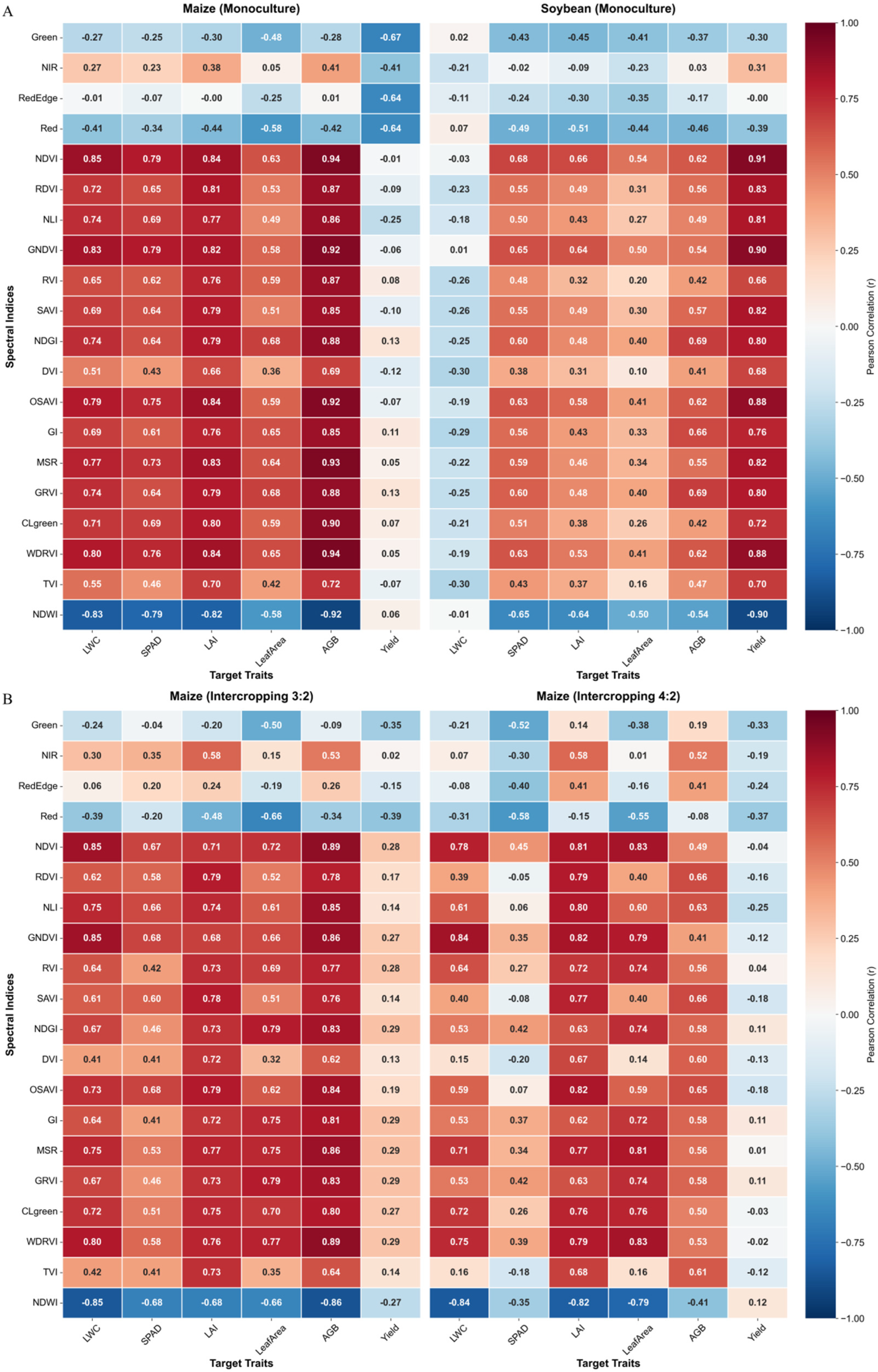
In this study, Pearson correlation coefficients were calculated to evaluate the linear response ability of 20 spectral indices to crop agronomic parameters (LWC, SPAD, LAI, leaf area, AGB, and yield) under different planting patterns. The overall analysis showed that differences in crop species and spatial planting configurations led to pronounced divergence in canopy spectral responses.

In the monocropping control group (Figure 2A), maize and soybean exhibited fundamentally different spectral response mechanisms. For monocropped maize (left panel of Figure 2A), spectral indices showed very high sensitivity to vegetative growth parameters. The correlation coefficients between NDVI, NDGI and aboveground biomass (AGB) reached 0.94 and 0.88, respectively, and their correlations with leaf area index (LAI) were also strong (0.84 and 0.79). This indicates that multispectral data can accurately capture changes in canopy structural attributes associated with maize vegetative growth. However, maize yield in monocropping systems was largely “decoupled” from most spectral indices. For example, the correlation coefficient between NDVI and yield was only −0.01, and several red-edge–based indices even showed weak negative correlations. These findings suggest that, in monocropped maize, dry matter partitioning during reproductive growth is regulated by multiple physiological processes, and final yield variability cannot be explained by simple linear relationships with canopy “greenness.” By contrast, monocropped soybean (right panel of Figure 2A) displayed strong synchrony between spectral features and yield. Correlation coefficients between indices such as NDVI, GNDVI, and NLI and yield generally exceeded 0.90 (e.g., NDVI vs. yield, r = 0.91). This is attributable to the high canopy closure in soybean stands and the strong coordination between biomass accumulation and pod development, which enables spectral signals to effectively reflect yield potential.

Strip intercropping altered the within-field distribution of light and temperature and modified border-row structure, leading to pronounced fluctuations in the spectral correlations of maize (Figure 2B). When comparing the two intercropping configurations, the 4:2 pattern (right panel) exhibited a markedly stronger capability for monitoring canopy structural parameters than the 3:2 pattern (left panel). Under the 4:2 configuration, the correlation coefficient between LAI and NDVI reached 0.91, which was much higher than that observed under the 3:2 configuration (0.71). From an agronomic perspective, the wider soybean strip (four rows) in the 4:2 system optimized light availability for maize border rows, resulting in a more expanded canopy structure and reduced soil-background effects within mixed pixels, thereby improving the inversion accuracy of LAI. Despite this improvement, yield prediction for intercropped maize still faced the problem of failure of linear models. In particular, under the 4:2 configuration, even though LAI was monitored with very high accuracy, the correlation coefficient between NDVI and yield was only −0.04, showing an essentially nonlinear relationship. In contrast, under the 3:2 configuration, NDVI retained a weak positive correlation with yield (r = 0.28). This contrast further confirms the complexity of yield formation in intercropped maize, where the dynamic balance between border-row advantage and interspecific competition makes simple linear regression inadequate for accurate prediction.

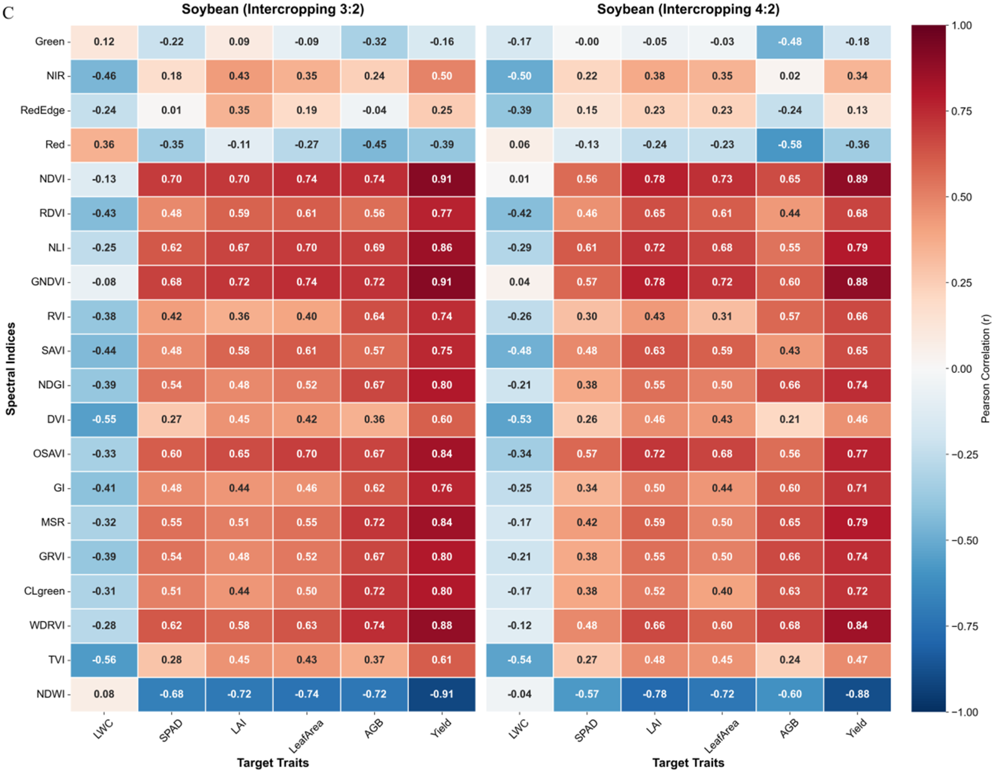
In contrast, intercropped soybean (Figure 2C) maintained very high spectral robustness within the complex planting system. Under both the 3:2 (left panel) and 4:2 (right panel) configurations, correlation coefficients between indices such as NDVI and GNDVI and yield consistently remained at high levels of around 0.90 (NDVI vs. yield: r = 0.91 for the 3:2 pattern; r = 0.89 for the 4:2 pattern). This indicates that the soybean canopy structure is relatively uniform, and vertical spectral signals are only marginally affected by shading from maize. Therefore, commonly used broadband vegetation indices are sufficient for yield estimation in intercropped soybean.

Taken together, the heatmap analysis clearly reveals the limitations of linear correlation analysis. Although soybean exhibited stable spectral–yield relationships under all planting configurations, the spectral response of maize yield was universally weak and unstable (|r| < 0.3). As shown in Figure 2B, even under conditions where LAI could be monitored with very high accuracy (r = 0.91), linear models still failed to predict yield. The widespread presence of this nonlinear “phenotype–yield” relationship suggests that simple regression based on a single spectral index cannot resolve the complex source–sink relationships within intercropping populations. Therefore, to overcome the bottleneck of linear regression, this study introduced machine-learning algorithms such as random forest (RF) and XGBoost to mine nonlinear combinations of multidimensional features, thereby achieving accurate inversion of crop phenotypes and yield under complex planting systems.

3.2. Estimation of Canopy Traits Under Different Cropping Systems

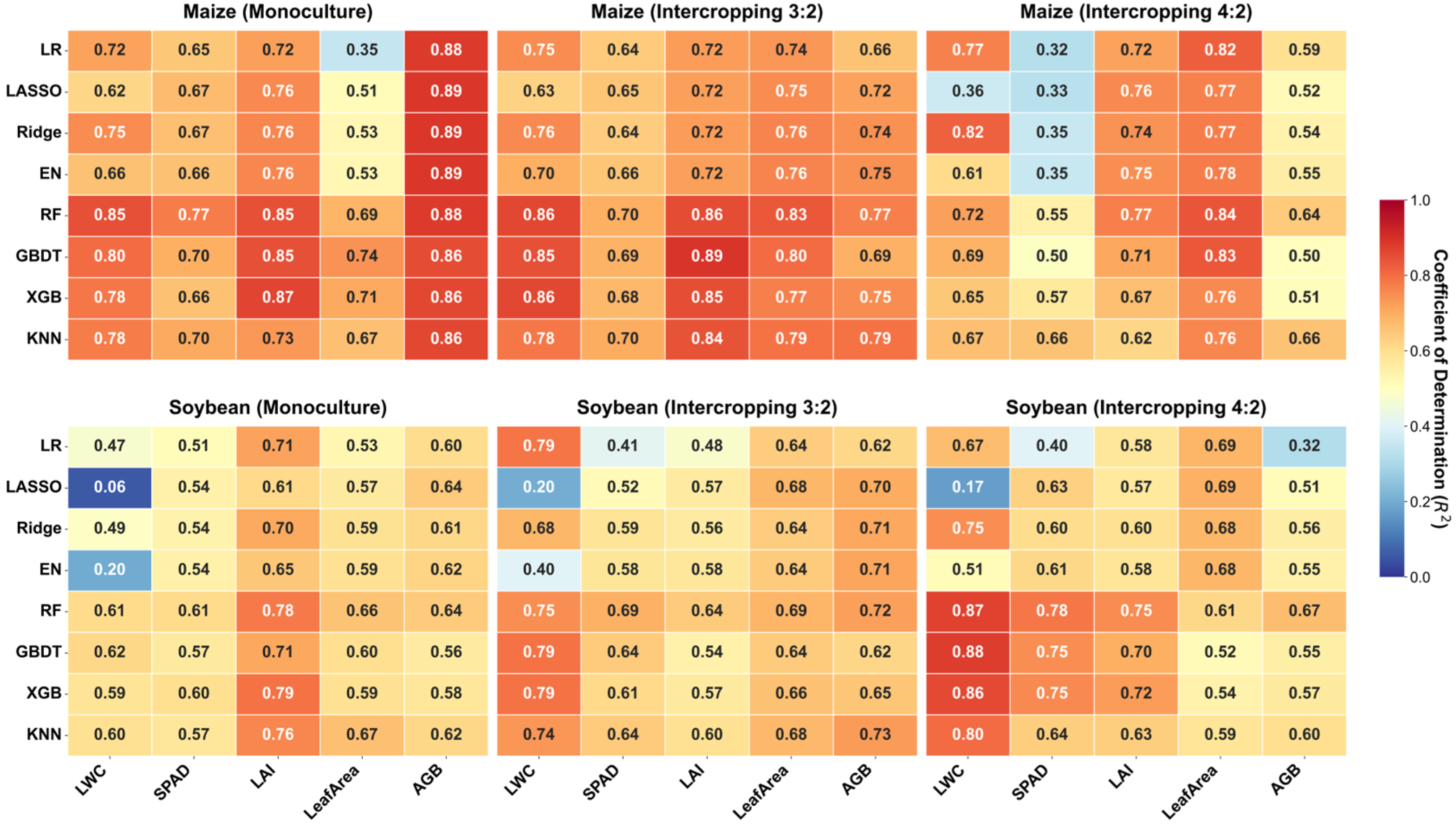
The heatmap of the coefficient of determination (R²) derived from five-fold cross-validation (Figure 3) revealed substantial performance differences among algorithms in capturing crop canopy spectral characteristics. The group of linear models (linear regression, Lasso, ridge regression, and elastic net) showed clear inadequacy when dealing with data from complex field environments. In particular, within highly heterogeneous intercropping systems, simple linear regression was unable to capture nonlinear spectral responses arising from mixed pixels and background noise. For example, in intercropped soybean under the 4:2 configuration, the Lasso model completely failed to invert LWC (R² = 0.17), and in monocropped maize, linear regression exhibited very weak explanatory power for leaf area (R² = 0.35). Such “lack-of-fit” phenomena confirm the inherent limitations of linear assumptions in multispectral remote-sensing inversion.

In contrast, nonlinear machine-learning algorithms markedly improved inversion accuracy by constructing high-dimensional feature spaces. The optimal inversion strategy exhibited distinct “crop–trait specificity.” In maize plots, the random forest (RF) algorithm showed the greatest robustness. Under both monocropping and 3:2 intercropping configurations, RF achieved the highest accuracy for AGB (R² = 0.88 and 0.86, respectively) and LWC (R² = 0.85 and 0.86, respectively), indicating that RF is particularly effective in handling the complex texture characteristics of high-biomass maize canopies. In soybean plots, gradient boosting decision trees (GBDT) and RF performed comparably, with scenario-dependent advantages. Under the most challenging 4:2 intercropping configuration, GBDT provided slightly higher accuracy for LWC (R² = 0.88) than RF (R² = 0.87), reflecting the superior capability of boosting algorithms to exploit subtle spectral variations in soybean subjected to shading stress. Analysis of the best-in-class models across scenarios further showed that canopy structural parameters were inverted with generally higher accuracy than biochemical parameters. For both maize and soybean, optimal models yielded R² values typically greater than 0.80 for LAI and AGB. This is mainly because canopy geometry directly controls physical scattering in the near-infrared region, resulting in higher signal-to-noise ratios, whereas the spectral responses of biochemical components such as LWC and SPAD are relatively weak and easily masked by canopy structural heterogeneity. Although intercropping increased inversion difficulty, the selected machine-learning models still maintained strong monitoring capabilities. In maize under the 4:2 intercropping configuration, AGB inversion accuracy declined because of pronounced border-row effects (optimal model: RF, R² = 0.64), while LAI estimation accuracy remained high (optimal model: RF, R² = 0.77). This strategy of selecting scenario-specific optimal algorithms effectively overcomes the adaptability limitations of single-model approaches in complex cropping systems and provides a solid methodological basis for subsequent high-precision mapping of phenotypic parameters.

3.3. Construction and Evaluation of Phenotypic Models Under Monoculture and Intercropping Conditions

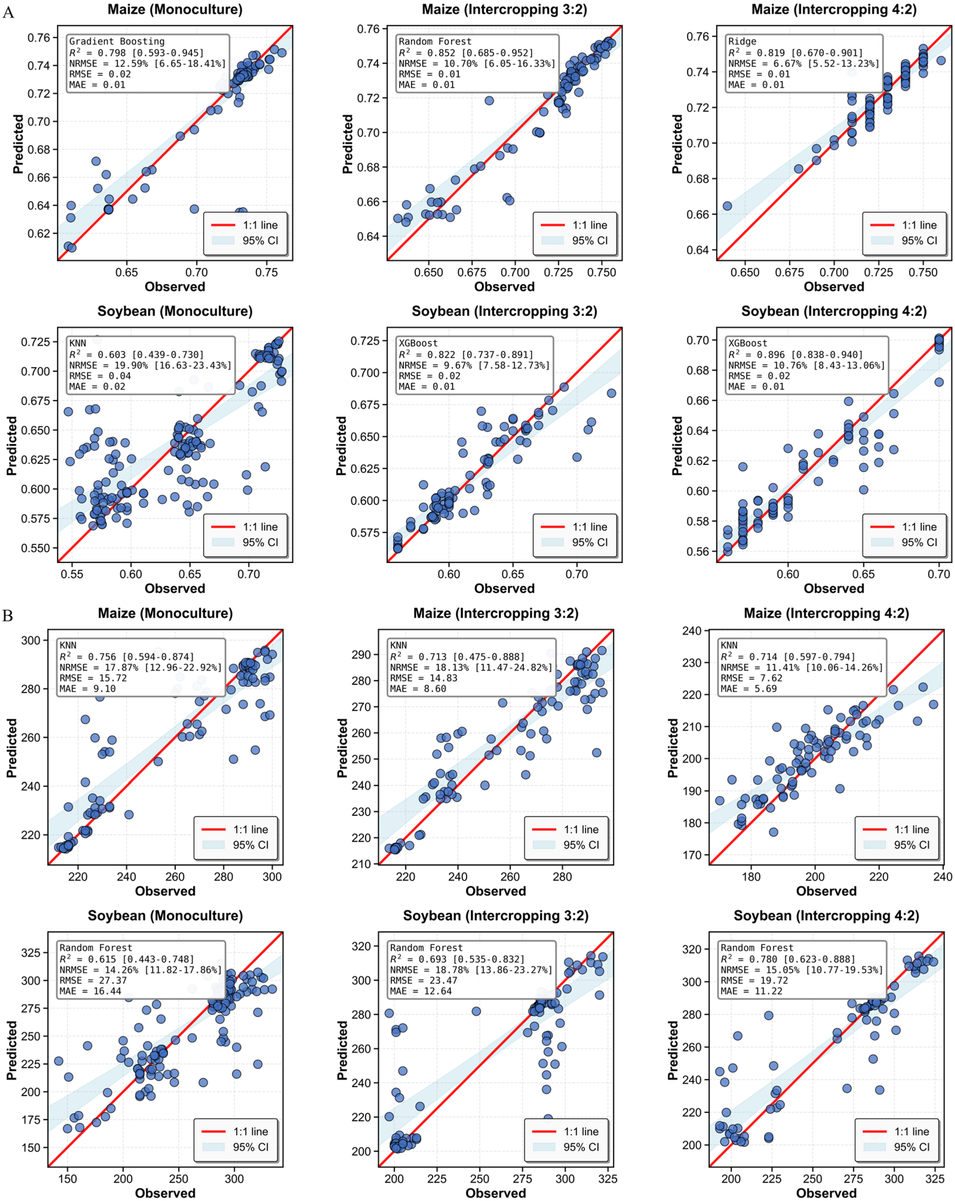
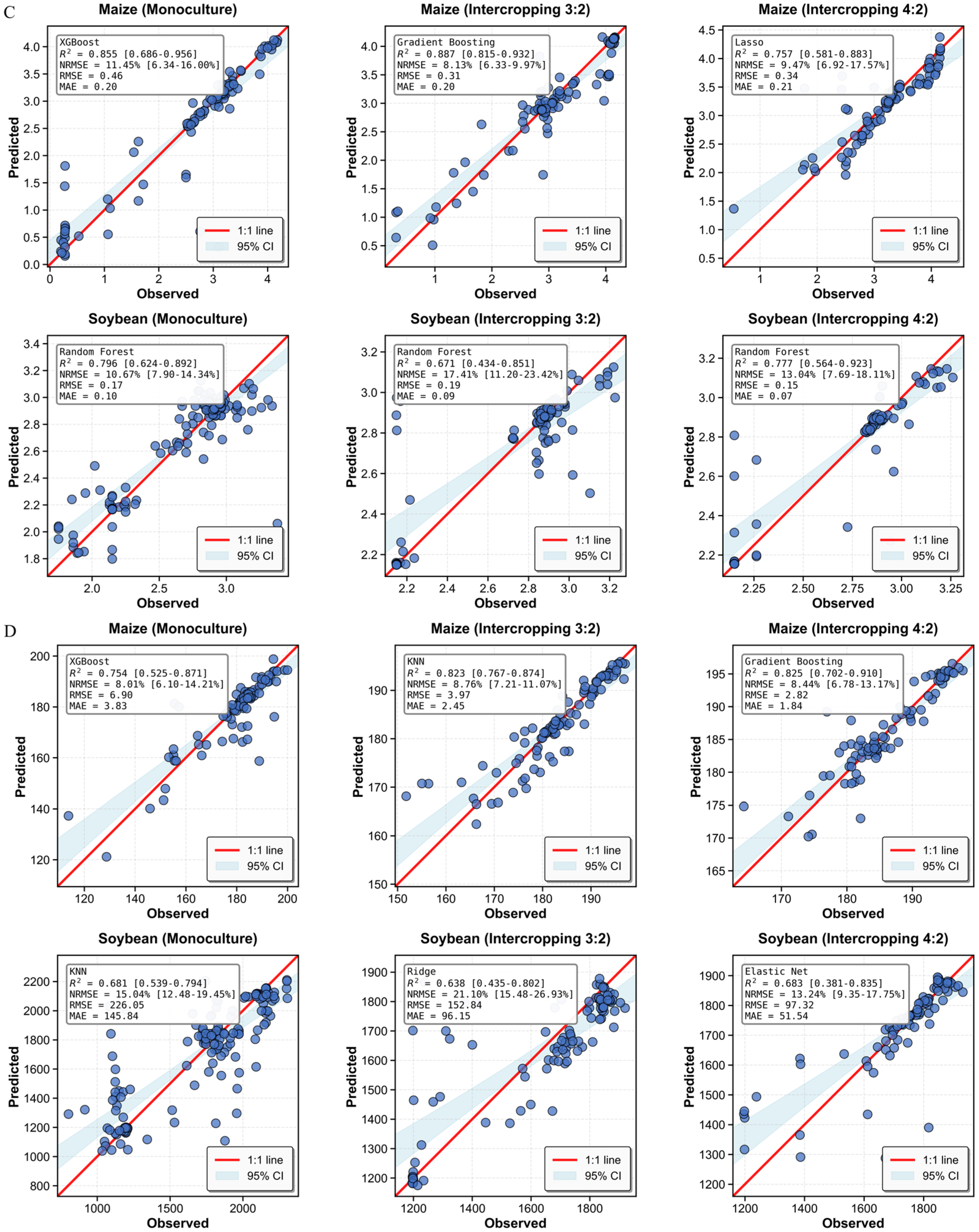
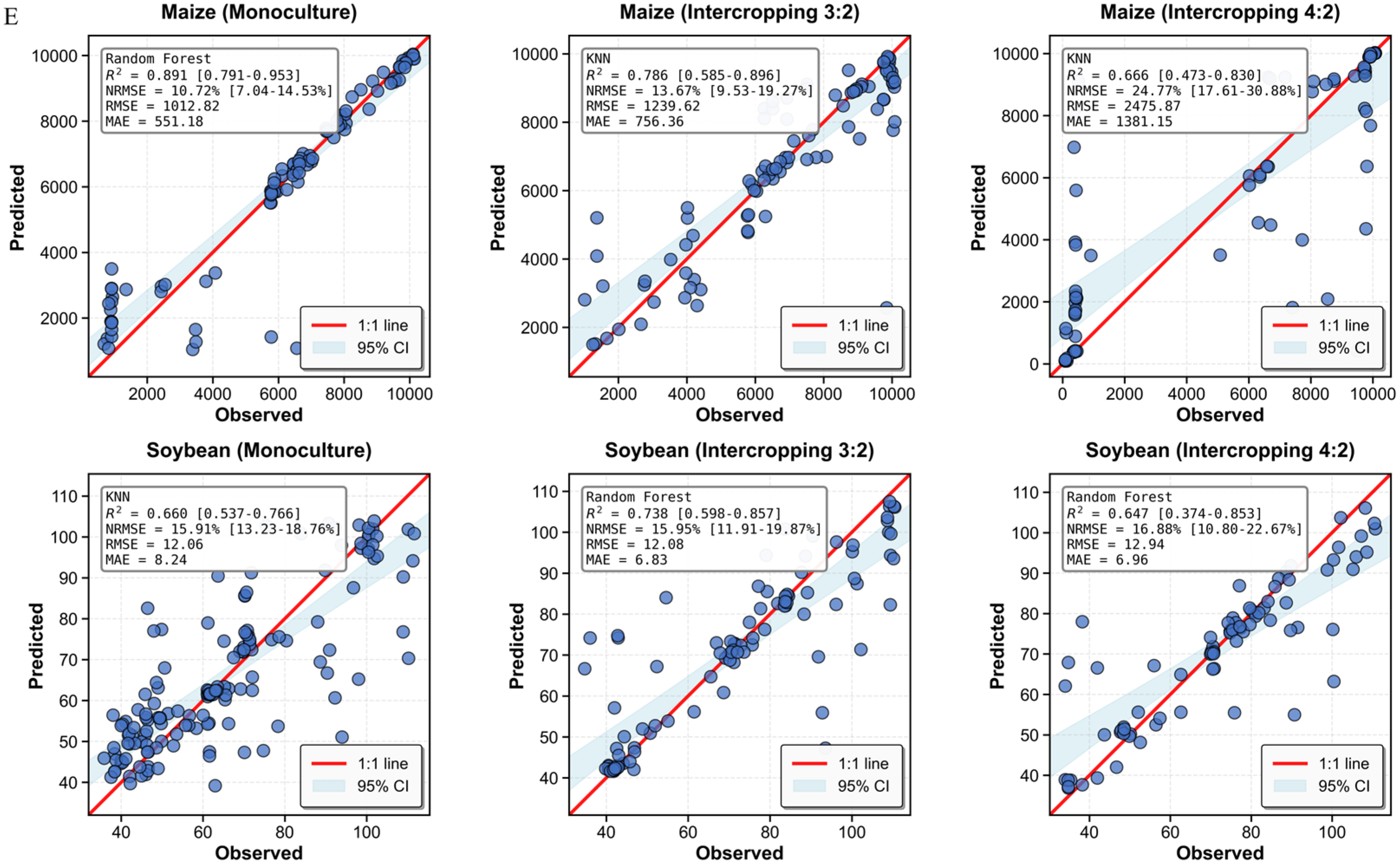
Based on the best-in-class models selected for each scenario, scatter plots of measured versus predicted values were generated for five key canopy phenotypic parameters (Figure 4). Overall, the prediction points were tightly clustered around the 1:1 line, and no obvious systematic bias was observed. This indicates that the strategy of selecting optimal inversion algorithms for specific “crop–pattern–trait” combinations effectively overcomes the adaptability limitations of a single model in complex intercropping systems.

For canopy structural parameters, high inversion accuracy was achieved overall because of their strong spectral scattering signals. Under the 3:2 maize intercropping pattern, the optimal gradient boosting (GBDT) model provided an excellent fit (R² = 0.891, NRMSE = 7.97%), effectively addressing the problem of signal saturation under high planting density (Figure 4C). For soybean, even under shading conditions in the 4:2 intercropping pattern, the random forest (RF) model maintained robust predictive capability (R² = 0.753, NRMSE = 13.72%) (Figure 4C). It is noteworthy that in high-biomass monocropped maize, the linear ridge model showed surprisingly high accuracy (R² = 0.890, NRMSE = 10.76%), indicating that, in monocropped fields where canopy structure is relatively uniform and not fully closed, regularized linear models are sufficient to capture biomass accumulation characteristics while avoiding overfitting by overly complex models (Figure 4E). In contrast, for intercropped soybean under the 3:2 pattern, the nonlinear KNN model performed better (R² = 0.728, NRMSE = 16.24%), effectively handling spectral nonlinearity caused by mixed pixels (Figure 4E). The capability of the models to predict individual leaf area (LeafArea) was consistent across crops. For maize, R² exceeded 0.73 under all planting configurations, with the RF model achieving high accuracy (R² = 0.838, NRMSE = 8.12%) under the 4:2 intercropping pattern (Figure 4D). For monocropped soybean, although the data showed slightly greater dispersion, the KNN model still achieved effective nonlinear fitting (R² = 0.668, NRMSE = 15.36%) (Figure 4D).

Compared with structural parameters, the inversion of biochemical parameters was more challenging; nevertheless, relatively high accuracy was still achieved through optimal model selection. The 4:2 intercropping pattern of soybean is generally considered difficult for inversion, yet the gradient boosting model achieved very high accuracy in this scenario (R² = 0.878, NRMSE = 11.66%), which was substantially better than that for monocropped soybean (R² = 0.617, NRMSE = 19.56%). This may be attributed to the more pronounced spectral responses of intercropped soybean under water stress, which can be effectively captured by boosting algorithms (Figure 4A). Interestingly, in maize under the 4:2 intercropping configuration, ridge regression (R² = 0.819, NRMSE = 6.67%) outperformed more complex machine-learning models because of its robustness to collinear features (Figure 4A). For chlorophyll content (SPAD), inversion accuracy was generally higher in maize plots than in soybean plots. For monocropped maize, the random forest model achieved the best performance (R² = 0.774, NRMSE = 17.20%) (Figure 4B). In contrast, data points for soybean were more dispersed, particularly under monocropping (R² = 0.609, NRMSE = 14.37%), reflecting the smaller variability of SPAD values in upper-canopy soybean leaves, which reduced spectral sensitivity (Figure 4B).The validation results in Figure 4 confirm that flexible selection of optimal inversion algorithms can maximize the application potential of UAV multispectral data across different planting patterns. This approach not only ensures high-accuracy inversion of structural parameters but also substantially improves the estimation accuracy of biochemical parameters under complex intercropping conditions.

3.4. Construction and Evaluation of Yield Models Under Monoculture and Intercropping Conditions

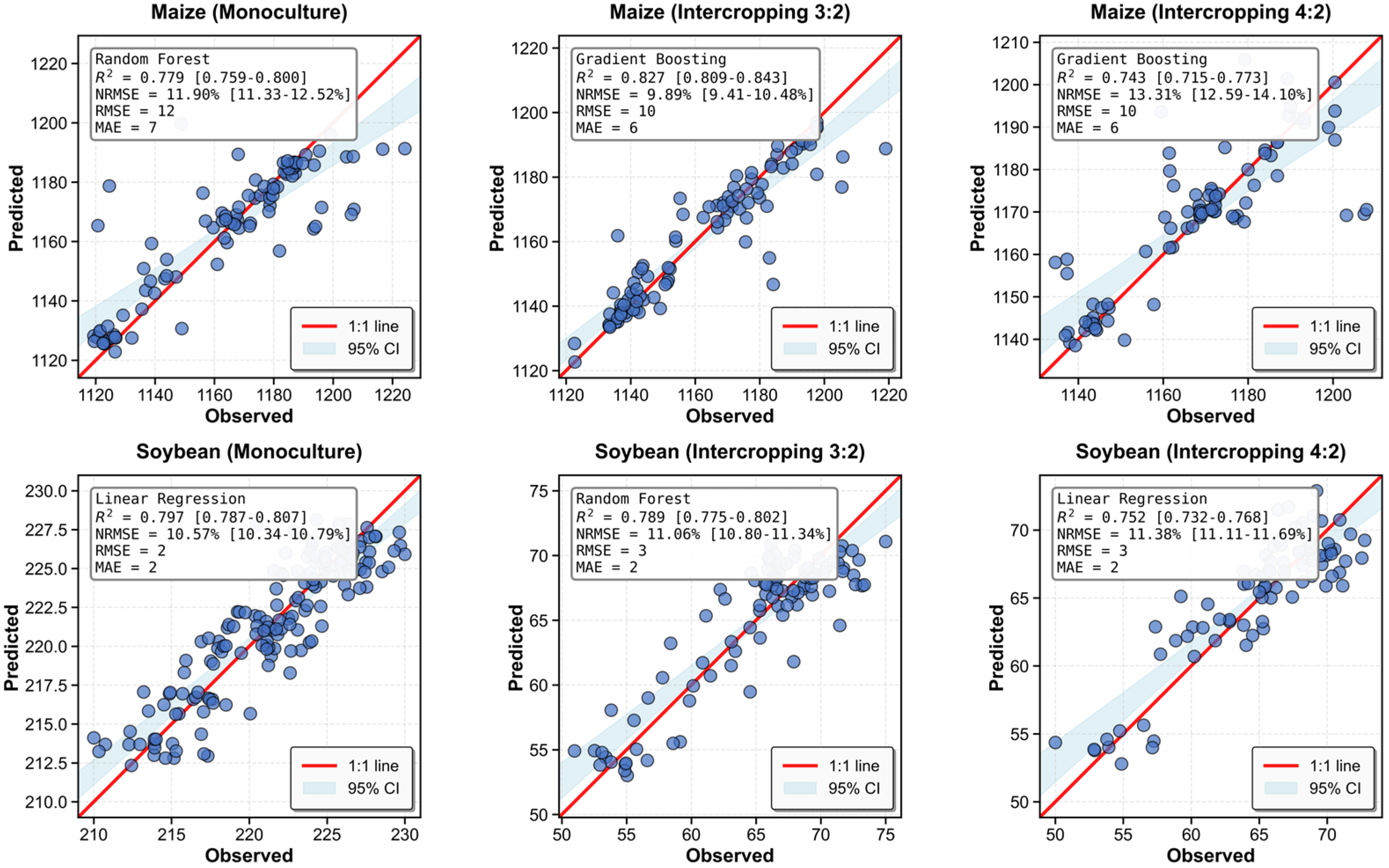
Given the nonlinear relationships between individual spectral indices and crop yield, yield prediction models were constructed using the best-performing machine-learning algorithms identified for each scenario. Validation results showed that these machine-learning models effectively resolved the complex mapping between canopy spectral signals and yield formation during the reproductive growth stage by constructing multidimensional feature spaces. In doing so, they overcame the applicability bottlenecks of linear models in yield prediction.

In maize plots, the optimal models exhibited high adaptability across spatial configurations and showed pronounced pattern dependence. Notably, under the 3:2 intercropping configuration, the gradient boosting (GBDT) model achieved the highest inversion accuracy (R² = 0.849, NRMSE = 9.28%), outperforming even the monocropping configuration (R² = 0.730, NRMSE = 13.17%) (Figure 5). This indicates that under the 3:2 row ratio, the GBDT algorithm can effectively capture yield gradients induced by strong border-row advantages and convert these structured biomass differences into identifiable spectral response signals. However, as spatial heterogeneity increased, model performance declined. Under the 4:2 intercropping configuration, although GBDT still retained explanatory capability for yield (R² = 0.687), prediction error increased (NRMSE = 14.78%). This suggests that wider strip widths and more complex inter-row competition disturb the stability of the relationship between canopy spectra and yield.

Soybean yield prediction models showed high consistency and strong resistance to interference across planting configurations. In monocropping systems, the KNN model achieved excellent performance (R² = 0.787, NRMSE = 10.84%), with points closely distributed around the 1:1 line, demonstrating the effectiveness of nonparametric methods for homogeneous canopies. In intercropping systems, despite the more complex assimilate allocation under shading imposed by maize, the RF model still achieved accurate yield predictions. Under the 3:2 configuration, model accuracy was comparable to or slightly higher than that of monocropping (R² = 0.793, NRMSE = 10.96%), and even under the most unfavorable light conditions in the 4:2 configuration, RF maintained high accuracy (R² = 0.724, NRMSE = 11.99%). These findings indicate that ensemble learning models incorporating red-edge and near-infrared bands can effectively extract “stay-green” characteristics of stressed soybean, establishing a robust linkage between spectral signals and final economic yield.

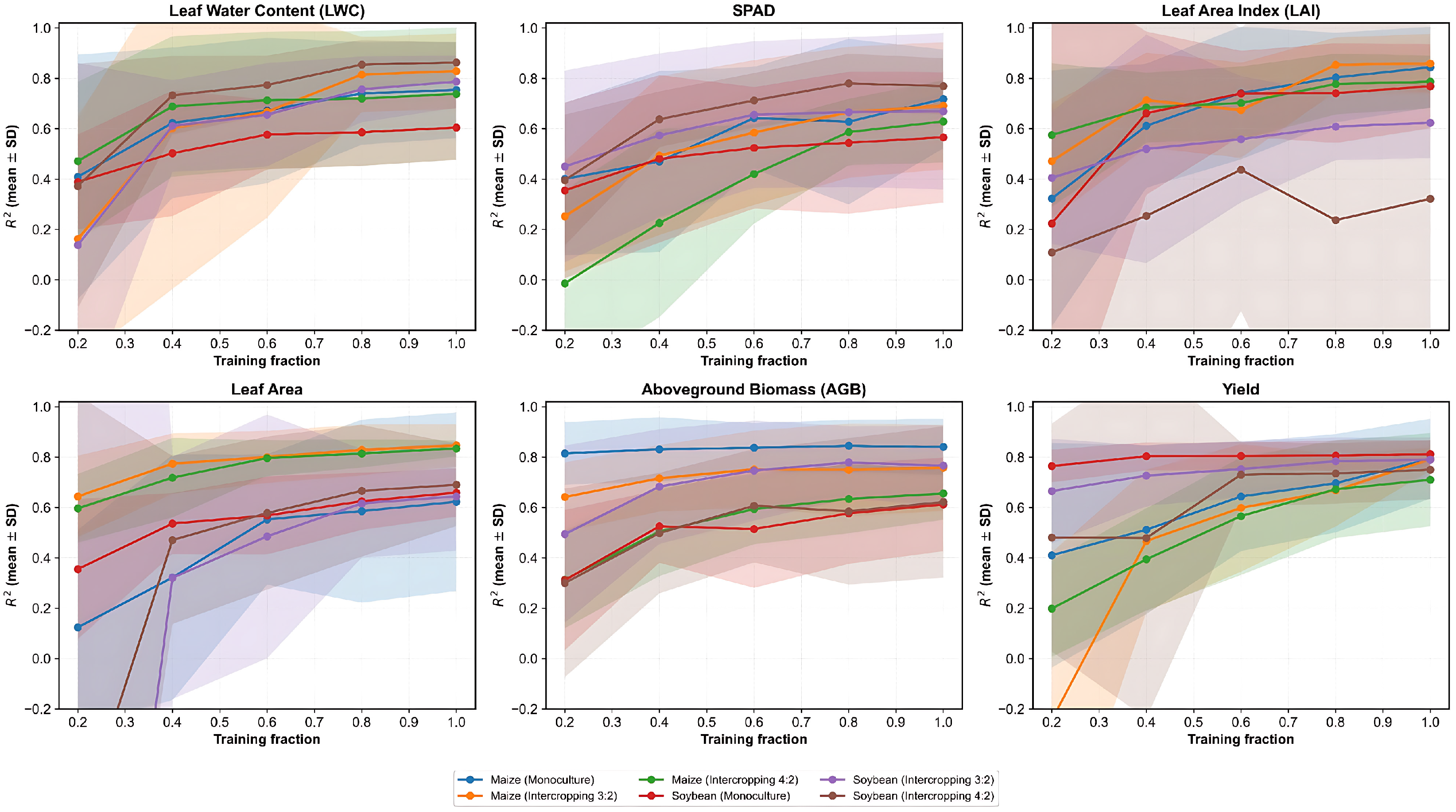
Learning-curve analysis (Figure 6) was conducted to evaluate sample-size adequacy and potential overfitting across six planting modes. For all five phenotypes and yield, the cross-validated R² generally increased with training fraction and tended to plateau at higher fractions, indicating that model performance becomes progressively more stable as more samples are used for training. The reduced variability (shaded ± SD) at larger training fractions further suggests improved robustness and a lower risk of overfitting. Notably, yield and canopy-structure–related traits (e.g., LAI and AGB) required larger training fractions to approach stable performance, implying higher complexity and/or stronger environmental and management heterogeneity in these targets.

3.5. Analysis of Explainability and Feature Mechanisms in Machine Learning Models

3.5.1. Feature Importance Analysis Based on SHAP Values

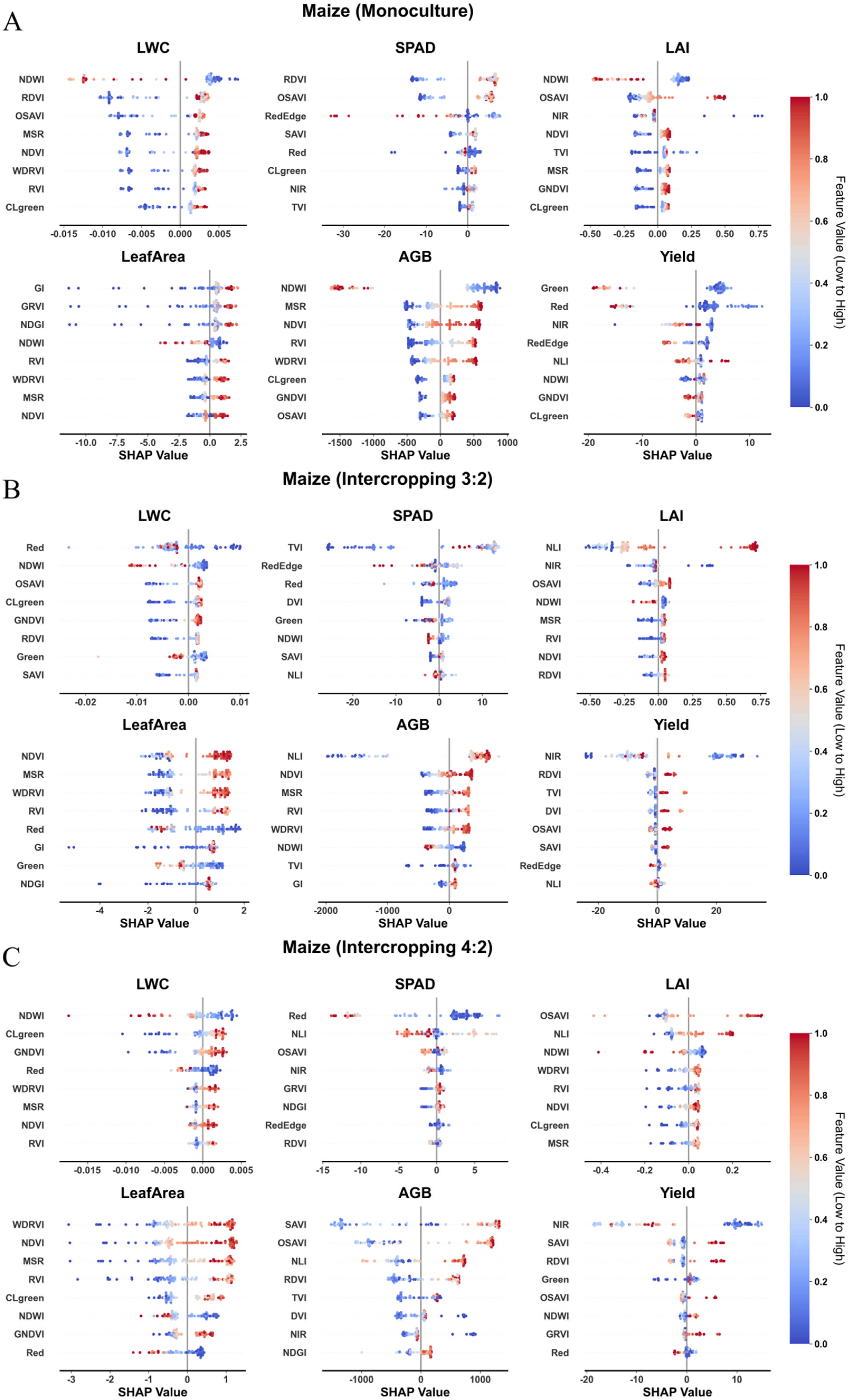
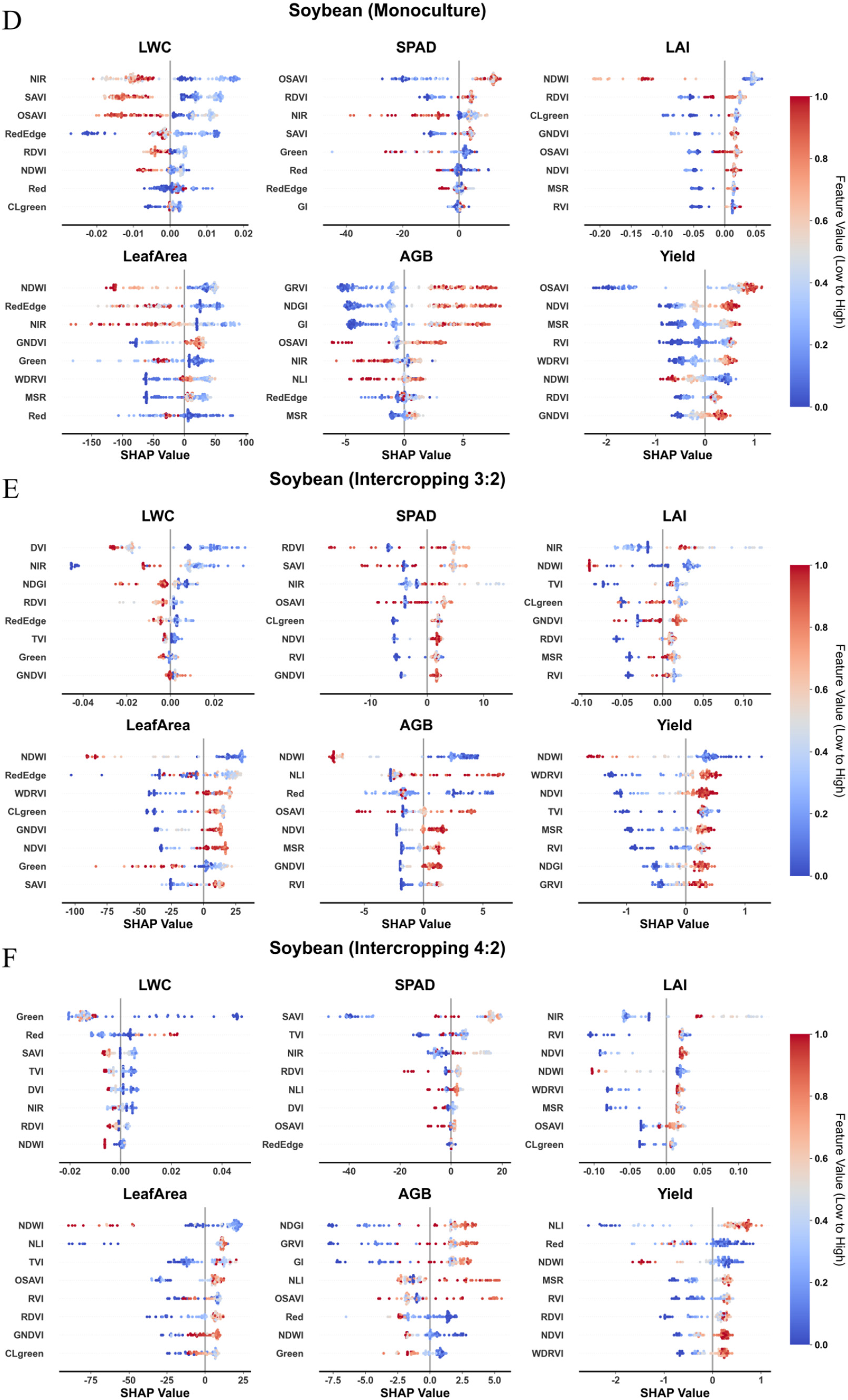
To investigate differences in spectral indicators associated with yield formation under different planting patterns, SHAP analysis was employed to quantify the contribution weights of multispectral features to yield prediction, thereby revealing the relative importance of population structural and physiological attributes under different spatial configurations (Figure 6). The results indicated that planting pattern altered the distribution of light–temperature resources and the interspecific competition regime in the field, forcing an adaptive shift in the yield response mechanism between “physiological-function dominance” and “canopy-structure dominance”.

In monocropped maize, where the light environment is homogeneous and interspecific competition is absent, individual plant growth is relatively uniform, and the major yield-limiting factor lies in the persistence of photosynthesis during the late reproductive stage. SHAP analysis showed that visible bands (green and red) and red-edge features exhibited the strongest explanatory power for yield (Figure 7A). Lower reflectance in the visible region corresponded to higher predicted yield, which agronomically reflects higher chlorophyll content in functional leaves and superior “stay-green” performance during the grain-filling period. This indicates that, in high-yield monocropping fields, delaying leaf senescence and maintaining high source activity is the key physiological basis determining final yield. By contrast, strip intercropping introduces strong border-row effects and interspecific competition, markedly increasing structural heterogeneity within the canopy. Under both the 3:2 (Figure 7B) and 4:2 (Figure 7C) configurations, the near-infrared band (NIR) and its derivative indices (e.g., SAVI and RDVI), which characterize canopy geometry and stand biomass, emerged as the primary predictors. This suggests that, under intercropping conditions, morphological–structural attributes such as plant height, stem diameter, and leaf area density, induced by border-row advantages, replace purely physiological indicators as the dominant determinants of yield. Notably, the high contribution rate of SAVI in the 4:2 configuration indicates that, under wider row spacing, accurately removing soil background noise and quantifying canopy light interception capacity are crucial for precise yield estimation.

The spectral response characteristics of soybean clearly reflected its morphological and physiological plasticity in adapting to different light environments. In monocropped soybean, early canopy closure and high stand density caused conventional spectral signals to saturate easily. Consequently, OSAVI and NDVI—both less sensitive to high biomass—became the dominant features distinguishing subtle differences among stands (Figure 7D), primarily by capturing variation in effective photosynthetic area beneath a closed canopy. After entering intercropping systems, shading stress imposed by maize strongly constrained soybean morphogenesis and assimilate allocation. Under the narrow-row 3:2 configuration (Figure 7E), NDVI re-emerged as the most important predictor and showed a strictly positive relationship with yield, indicating that, under conditions where biomass accumulation is limited by strong interspecific competition, maintaining basic canopy greenness and vegetative size constitutes the physiological foundation for yield formation. In contrast, under the relatively improved light environment of the 4:2 configuration (Figure 7F), the nonlinear index NLI and the red band contributed substantially more to yield prediction. Agronomically, this reflects physiological compensation to shade: soybean adapts to low-light conditions by increasing specific leaf area (SLA) or exhibiting leaf yellowing (chlorophyll dilution). Changes in red-band reflectance sensitively captured these stress symptoms, such as chlorosis and etiolation, thereby linking spectral responses to underlying physiological constraints.

3.5.2. Nonlinear Response of Key Features to Yield Using PDP

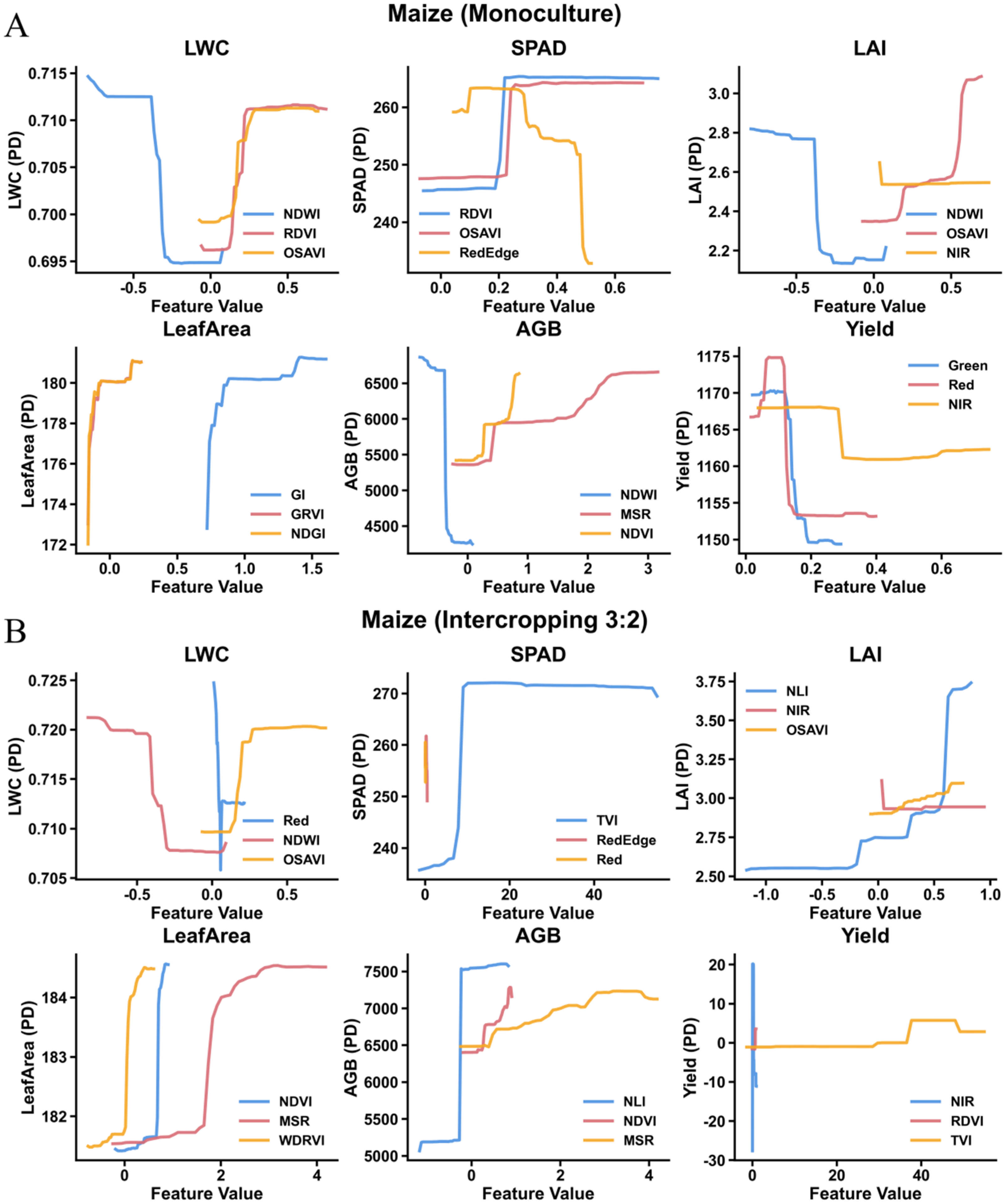
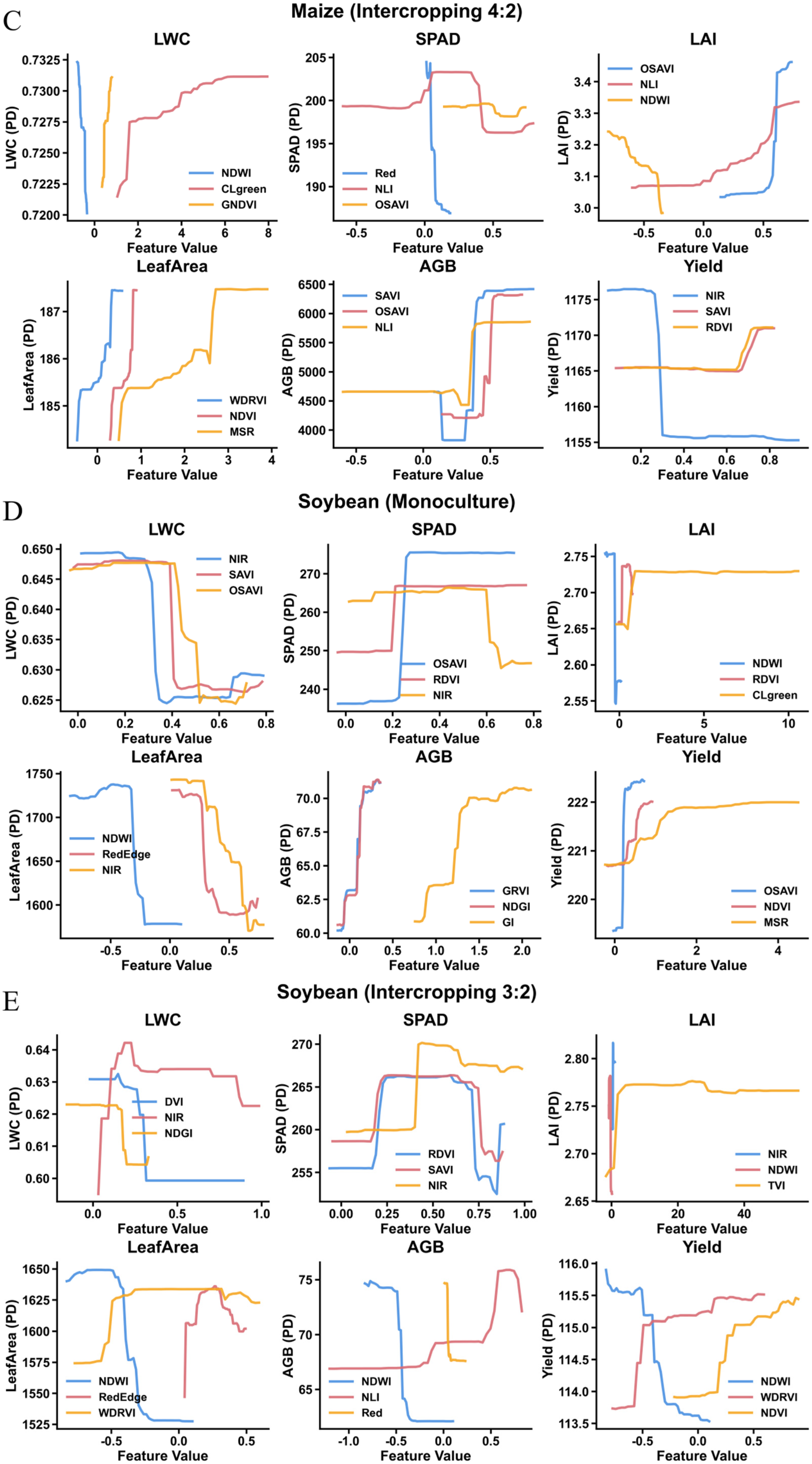
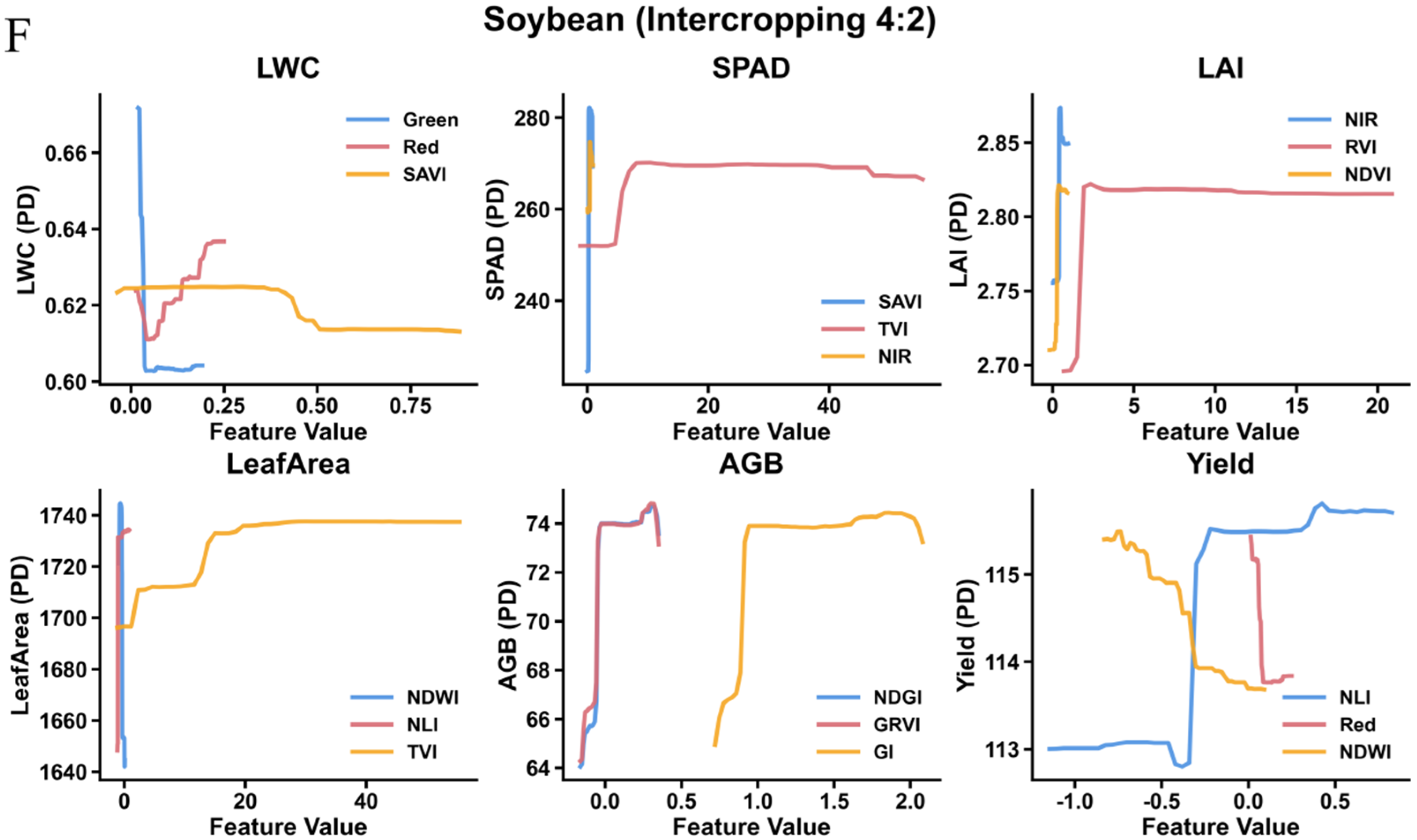
While SHAP analysis identified the ranking of yield-driving factors under different planting patterns, partial dependence plots (PDPs) were further used to quantify the marginal effects of these factors on yield. The results showed that the “phenotype–yield” relationships did not follow a uniform linear pattern across planting modes; instead, they exhibited pronounced features of physiological saturation, structural compensation, and survival thresholds (Figure 8). These nonlinear responses provide a biological explanation for the failure of linear models in complex intercropping systems.

In monocropped maize (Figure 8A), the PDP curves revealed a widespread “source–sink limitation” in high-yield stands. Using the green band as a representative dominant feature, the yield response to green reflectance exhibited a clear L-shaped pattern. Within the low-reflectance range (<0.20, corresponding to high chlorophyll content), yield increased markedly with increasing canopy greenness. However, when reflectance decreased further to below 0.05, the response curve approached a plateau. This pattern indicates that, in high-yield monocropping fields, further enhancement of photosynthetic capacity does not translate linearly into additional yield gain, as the limiting factor shifts from photosynthetic source activity to sink capacity. Linear regression models fail to capture this signal saturation at high values, resulting in systematic misestimation of high-yield samples.

In intercropped maize, the mechanisms of yield formation exhibited pronounced spatial heterogeneity. Under the 3:2 configuration (Figure 8B), the NIR feature showed a relatively stable, approximately linear yield gain, reflecting a balance between interspecific competition and border-row advantage in this planting pattern. By contrast, under the 4:2 configuration, where spatial heterogeneity was greatest (Figure 8C), the response of yield to SAVI displayed a distinctive “step-like” pattern. The curve exhibited a sharp increase at SAVI ≈ 0.25, followed by maintenance at a high level in the upper range. This S-shaped decision boundary reveals the model’s filtering mechanism for soil background noise: in zones with low vegetation cover induced by wide row spacing, the model suppresses spurious contributions from bare soil; once the signal exceeds the vegetation–soil discrimination threshold, the model rapidly responds to the structured biomass gains driven by border-row advantage.

In monocropped soybean (Figure 8D), the PDP curve of OSAVI exhibited an evident plateau in the high-value range (>0.60). This represents a typical canopy-closure effect: as the canopy closes, mutual leaf shading reduces the sensitivity of spectral signals to further increases in biomass. In this highly closed-canopy zone, the model produced conservative and robust predictions, effectively avoiding overfitting.

In contrast, the spectral responses of intercropped soybean revealed the physiological limits of plants under low-light stress. Under the narrow-row 3:2 configuration (Figure 8E), NDVI showed a strictly monotonic increasing relationship with yield, indicating that under conditions of photosynthetic “starvation,” every incremental increase in green leaf area was directly converted into yield accumulation. However, in the 4:2 configuration, where shading stress was most severe (Figure 8F), the response curve of the nonlinear index NLI exhibited an abrupt threshold shift. When NLI dropped below a critical value (approximately −0.5), the predicted yield declined precipitously. This mathematical pattern characterizes a physiological tipping point: once light conditions deteriorate beyond the limits of morphological plasticity, soybean can no longer maintain basic carbon assimilation to offset respiratory consumption, leading to a systemic collapse in yield formation capacity.

3.6. Spatial Distribution Patterns and Variability Analysis of Crop Yield Under Different Planting Patterns

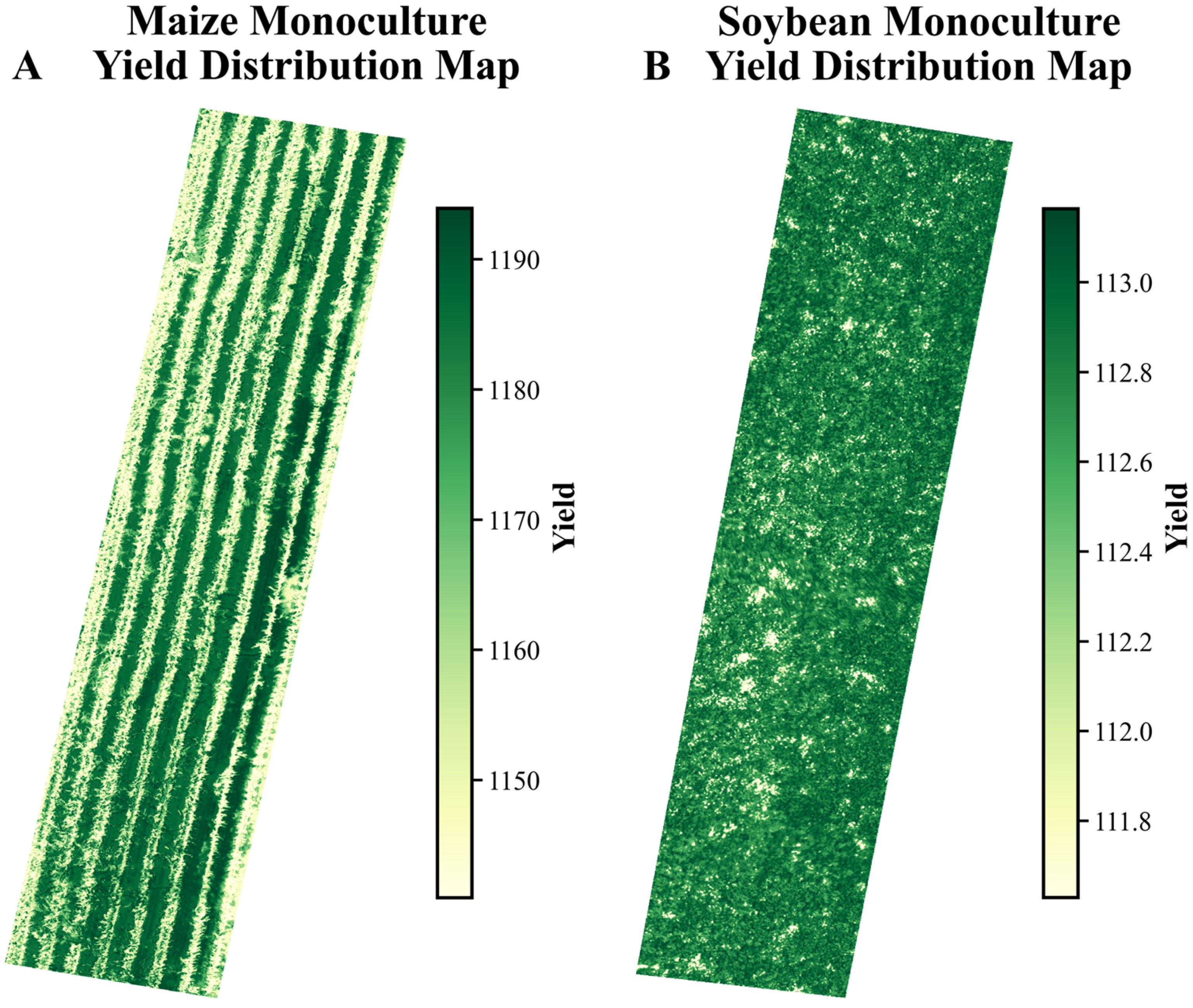
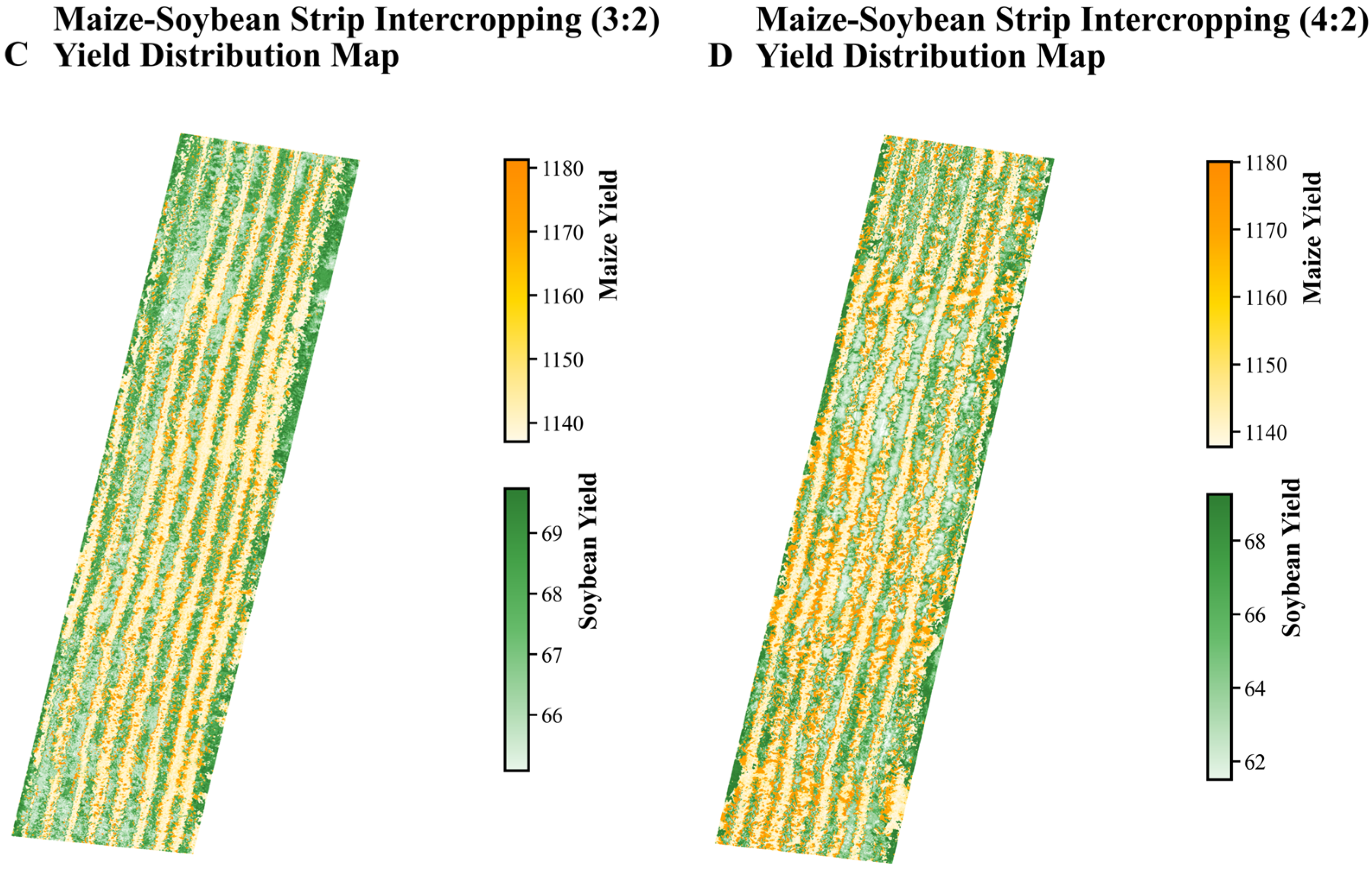
Based on the optimal machine-learning models, centimeter-resolution spatial yield maps were generated for each field (Figure 9). Distinct differences were observed in the spatial characteristics of yield formation between monocropping and intercropping systems. In monocropped maize (Figure 9A) and monocropped soybean (Figure 9B), high- and low-yield zones exhibited irregular “patchy” distributions without obvious geometric regularity. This unstructured spatial variability is mainly attributed to the inherent heterogeneity of soil fertility, microtopography, and water distribution within fields. These results indicate that, in single-crop systems, the background soil environment is the dominant factor shaping the spatial pattern of yield.

By contrast, the maize–soybean strip intercropping systems (Figure 9C,D) exhibited strong and highly regular strip-shaped spatial heterogeneity, reflecting the reshaping of yield formation by interspecific interactions. In both the 3:2 and 4:2 intercropping configurations, pronounced border effects were observed in the spatial distribution of crop yields. As indicated by the deeper orange tones in Figure 8, maize border rows adjacent to soybean displayed higher yield than inner rows, confirming that tall crops, by occupying an ecological niche advantage, intercepted more lateral radiation and exploited marginal soil resources, thereby generating a significant border-row yield increase. In contrast, in the green-toned soybean strips, shading from adjacent tall maize plants led to lighter colors along strip edges, indicating yield suppression and producing a concave-shaped spatial distribution opposite to that of maize.

These high-resolution yield maps demonstrate that uniform field management is poorly suited to the complex spatial variability of intercropping systems. Based on the patterns revealed in Figure 8, field management should adopt site-specific, variable-rate practices: for maize border rows with clear yield advantages, water and nutrient inputs may be moderately increased to exploit yield potential; for soybean border rows with severe shading, emphasis should be placed on chemical growth regulation, lodging prevention, and disease monitoring. The remote-sensing inversion framework proposed in this study can accurately identify such micro-scale variability and thus provides robust data support for fine-scale agronomic decision-making in strip intercropping systems.

4. Discussion

4.1. The Mechanism of Cultivation Patterns Affecting the Accuracy of Crop Yield Inversion

This study revealed a pronounced spatial-configuration dependence in the accuracy of yield inversion based on UAV multisource data. Notably, maize yield estimation accuracy was highest in the 3:2 intercropping configuration (R² = 0.849), exceeding that of maize monocropping (R² = 0.730) and the 4:2 intercropping configuration (R² = 0.687). This finding differs from earlier studies that suggested that the high heterogeneity of intercropping systems weakens remote-sensing inversion performance [9] but is consistent with more recent evidence linking border effects in intercropping systems with enhanced spectral responses [5].

This phenomenon may be partly attributable to the coupling between canopy structure and spectral response, which can modulate the sensitivity of spectral indices to yield-related variations. We note that other factors (e.g., micro-environmental conditions, soil heterogeneity, and management-related variability) may also contribute, and disentangling their relative contributions warrants further investigation. In the 3:2 intercropping configuration, the maize strip is relatively narrow, and the pronounced border-row effect induces a distinct biomass gradient in maize canopies during the reproductive growth stage [53]. This structured variation arising from interspecific competition generates highly discriminative spectral signals in the red-edge and near-infrared bands, which in turn provide richer feature information for machine-learning models than the more homogeneous monocropped canopy. However, in the 4:2 configuration, the wider maize strip increases the proportion of interior rows and dilutes border effects; consequently, within-strip self-shading becomes more pronounced, leading to stronger effective intraspecific competition, greater spectral mixing within the canopy, and a weakened border-row–induced signal enhancement, thereby reducing inversion accuracy. This observation is in line with Liu et al. [6], who reported reduced stability of remote-sensing monitoring under overly wide strip layouts. In our case, the reduced stability is mainly attributed to the increased proportion of interior rows and enhanced within-strip self-shading, which amplify illumination-driven variability (e.g., shadowing and BRDF effects) and strengthen canopy-structure heterogeneity, thereby increasing pixel-level variability and weakening the border-row signal enhancement. We note that this effect can be context-dependent (crop type, canopy architecture, solar geometry, and spatial resolution) and should not be interpreted as universally applicable. For soybean, although shading stress from maize alters its light environment, the Random Forest model maintained high prediction accuracy in both the 3:2 and 4:2 configurations (R² > 0.72). This suggests that, although weak light conditions modify soybean architectural traits (e.g., slender stems and thinner leaves), the key spectral responses of the canopy remain robustly coupled with final yield through a stable allometric relationship. This finding is consistent with the results of Feng et al. [34], confirming that multispectral remote sensing can effectively capture the critical variability of crop productivity even when plant morphology is strongly shaped by phenotypic plasticity.

4.2. The Advantages of Machine Learning Algorithms in Analyzing Complex Canopy Spectral Signals

The complexity of intercropping systems arises from nonlinear light competition and microenvironmental variation, which cause single vegetation indices (such as NDVI) to saturate easily at high biomass levels. The results of this study showed that ensemble learning algorithms based on multi-feature fusion (GBDT and Random Forest) significantly outperformed traditional linear regression models in yield inversion accuracy. This conclusion provides strong support for the viewpoint of Li et al. [54], who suggested that nonlinear models have broad applicability in complex crop-monitoring scenarios.

Specifically, the superior performance of the GBDT algorithm in the 3:2 maize intercropping system can be attributed to its strong capability for learning nonlinear features. Compared with single-parameter models [26], GBDT flexibly partitions the high-dimensional feature space generated by border-row effects through a gradient boosting strategy, accurately capturing yield-related nonlinear mutations. In addition, when processing low-light data in the 4:2 soybean intercropping system, the Random Forest algorithm exhibited excellent noise resistance. Because intercropped canopies contain numerous mixed pixels (soil, shadow, and vegetation), conventional regression models are highly prone to overfitting. In this study, the bagging-based aggregation of multiple trees in RF helped reduce prediction variance and improve robustness to mixed-pixel noise (soil–shadow–vegetation), which is consistent with Li et al. [55], who reported the strong noise-tolerance and generalization ability of RF when modeling crop variables from high-resolution remote-sensing features under heterogeneous canopy conditions. Together, these findings indicate that ensemble-learning algorithms offer an effective solution to the “mixed-pixel” problem in intercropping systems.

We acknowledge a practical gap between centimeter-scale analytics and meter-scale mechanization. Although UAV imagery enables centimeter-resolution mapping, most conventional spreaders and sprayers operate at meter-scale widths, which limits immediate row-level variable-rate application in mixed cropping. Therefore, centimeter-scale outputs are best treated as a diagnostic layer and should be aggregated into strip- or zone-level management units that match available equipment. Row-level differentiation would require row-selective applicators or robotic platforms, representing an important barrier to implementation and a priority direction for future work.

4.3. Implications of Spatial Patterns in Crop Yield Distribution for Precision Agricultural Management

The centimeter-scale yield maps generated in this study clearly revealed two distinct mechanisms of spatial variability—“soil-driven” and “competition-driven”—providing a new perspective for precision management in intercropping systems. However, the operational use of such centimeter-scale analytics requires aggregation into management units consistent with the working width and actuation capability of available machinery (typically meter-level).

In monocropping systems, yield variation primarily appeared as irregular patches, which is generally driven by spatial heterogeneity in soil background conditions (e.g., organic matter and moisture) [13]. Therefore, management of monocropped fields should focus on soil map–based variable-rate fertilization (VRT). In contrast, intercropping systems exhibited a highly regular, alternating-strip spatial pattern of variability imposed by the strip layout. The maps showed that maize border rows had significantly higher yields than inner rows, whereas soybean border rows were suppressed; these patterns support an interpretation consistent with the proposition proposed by Wang et al. [12] that interspecific complementarity and competition can coexist in intercropping systems.

On this basis, we propose that strip- or zone-based differentiated management should be adopted in intercropping systems by aggregating centimeter-scale analytics into actionable management units; where suitable equipment is available, this can be implemented as strip-differentiated operations in mechanized farming. For maize border rows with substantial yield potential, uniform fertilization should be abandoned in favor of targeted topdressing to further exploit yield advantages. For soybean border rows experiencing severe shading, management should not blindly pursue biomass accumulation; instead, priority should be given to chemical growth regulation, lodging prevention, and disease monitoring [4]. The high-precision UAV-based remote-sensing inversion methodology proposed in this study can rapidly and non-destructively identify such spatial variability, providing essential data support for agronomic decision-making refined down to the row scale.

4.4. Research Limitations and Future Prospects

Despite successfully demonstrating the effectiveness of machine-learning algorithms for yield inversion in intercropping systems and revealing spatial heterogeneity under different planting configurations, this study still has several limitations owing to the restricted temporal span of the experimental dataset. To address restricted temporal coverage, future work will extend the observation window by integrating multi-source time series and complementary information. Specifically, (i) multi-sensor data fusion (e.g., combining UAV observations with satellite time series) can provide denser temporal sampling; (ii) gap-filling and imputation methods can be used to reconstruct continuous vegetation-index/spectral trajectories when flights are missing due to weather or operational constraints; and (iii) remote-sensing features can be coupled with on-site meteorological measurements and simple crop/soil process constraints to reduce year-specific weather dependence and improve generalization. In addition, hyperspectral imaging and multi-season datasets will be explored to better capture physiological variation and strengthen cross-year validation. These issues should be further addressed in future research.

First, the robustness of the models to interannual climatic variability remains to be validated. Crop growth is a dynamic process that is highly sensitive to environmental stresses, and the relationship between spectral responses and final yield may fluctuate across years with differing rainfall distribution, temperature accumulation, and extreme weather events [54]. As the data used in this study were mainly derived from a specific experimental year, the generalizability of the models across different climatic conditions (e.g., dry versus wet years) requires further verification through long-term field observations. Future research should aim to construct a multi-year “all-scenario spectral feature library” and explore the interannual drift of crop growth parameters to improve model stability in long-term monitoring. Therefore, the current results should be interpreted as a pilot study, and cross-year validation (e.g., training on one year and testing on another, or leave-one-year-out evaluation) is required before claiming interannual robustness.

Second, the spectral resolution of multispectral sensors limits the capacity to elucidate fine-scale physiological mechanisms. Although this study confirmed the key role of the red-edge band in improving inversion accuracy, conventional multispectral sensors have relatively wide bandwidths (10–40 nm), making it difficult to capture subtle variations in chlorophyll fluorescence (SIF) or carotenoid absorption characteristics under shaded conditions in intercropped soybean [56]. To better characterize the photosynthetic physiological responses of shaded soybean, future research may incorporate hyperspectral imaging, which offers nanometer-level spectral resolution. This would enable extraction of narrowband features closely related to light-use efficiency (LUE), thereby providing deeper insight into the “spectrum–yield” response mechanisms in intercropping populations.

Finally, purely data-driven models lack mechanistic interpretation of yield-formation processes. Although GBDT and Random Forest achieved high predictive accuracy, they essentially remain “black-box” models that cannot explicitly quantify the contributions of specific environmental factors to yield accumulation. Future work should therefore move toward mechanism–data dual-driven frameworks, attempting to assimilate physiological parameters from crop growth models (e.g., APSIM or DSSAT) with remote-sensing observations. Such integration would retain the computational efficiency of machine learning while endowing models with explicit agronomic interpretability, thereby enabling dynamic prediction and scenario simulation of productivity in intercropping systems.

5. Conclusions

This study focused on the challenges of strong canopy structural heterogeneity and severe spectral mixing in maize–soybean strip intercropping systems, evaluated the potential of UAV multispectral imagery combined with machine-learning algorithms for yield estimation, and further elucidated the agronomic mechanisms underlying the “spectral–yield” relationships under different spatial configurations. The main conclusions are as follows:

(1) Ensemble learning algorithms overcame the applicability bottleneck of linear models in complex intercropping systems. The study demonstrated that the nonlinear “source–sink” relationships inherent in intercropping canopies make it difficult for traditional linear regression models to capture yield variability under mixed pixels. In contrast, ensemble learning algorithms (Random Forest and GBDT) effectively addressed nonlinear mapping by constructing high-dimensional feature spaces. Specifically, the GBDT model accurately captured the biomass gradient induced by strong border-row advantages in the maize 3:2 pattern (R² = 0.849), while the Random Forest model maintained high within-season stability in the most severely shaded soybean 4:2 pattern (R² = 0.724), enabling accurate yield inversion under complex planting configurations.

(2) Spatial configuration drove an adaptive shift in the spectral–yield response mechanisms. Explainable AI analyses based on SHAP and PDP revealed essential differences between monocropping and intercropping systems. Yield formation in monocrops was mainly driven by physiological traits—such as stay-green characteristics represented by visible bands—whereas yield prediction in intercropping shifted toward structural traits (e.g., biomass indicated by NIR and SAVI) and stress responses (e.g., shade-avoidance signals revealed by Red and NLI). This finding mechanistically explains why simple vegetation indices often fail in intercropping systems and highlights the necessity of constructing multidimensional feature spaces for complex crop monitoring.

(3) High-resolution yield maps highlighted the necessity of band-specific differentiated management. Centimeter-level yield maps clearly distinguished two fundamentally different drivers of spatial variability: monocropping fields exhibited irregular patchy distributions dominated by soil background heterogeneity, whereas intercropping systems showed regular banded patterns controlled by interspecific competition and complementarity. Accordingly, field management in intercropping systems should move beyond uniform treatment and adopt differentiated zone-specific operations. In the near term, the centimeter-scale maps should be translated into strip- or zone-level prescriptions that match the working width of conventional sprayers/spreaders, enabling differentiated management at a practical meter scale. True row-level- or border-row-selective operations in mixed cropping would require row-selective applicators or robotic platforms, which currently remains a key barrier for large-scale implementation. The proposed framework not only enables nondestructive yield estimation but also provides essential spatial guidance for precision agronomic decision-making in strip intercropping systems.