Hyperspectral Wavelength Selection Based on Inter-Class Feature Differences for Maize Seed Age Discrimination

Abstract

Maize is a globally major crop; however, the prevalence of mixed-aged seeds in the market complicates consumer selection and impedes the healthy development of the maize industry. This study introduces a novel method for identifying maize seeds of different storage ages. Seeds were categorized into three age groups: new seeds, one-year stored, and two-year stored, with 300 seeds per group. Hyperspectral images of all 900 samples were acquired using a visible and near-infrared (Vis-NIR) hyperspectral imaging system. To achieve optimal results with minimal spectral data, a feature wavelength selection algorithm based on Inter-Class Feature Differences (IFD) was proposed. When only using the selected three key wavelengths, combined with the linear discriminant analysis (LDA) algorithm, the discrimination accuracy among three different age groups reached 85.67%, while the discrimination accuracy between new and aged seeds achieved 95.33%. Compared to two commonly used variable selection algorithms—Successive Projections Algorithm (SPA) and Random Frog (RF), the proposed IFD method demonstrated superior performance when only a limited number of key wavelengths were used for modeling. These results indicate that the proposed algorithm offers an effective and efficient solution for maize seed age discrimination, showing great potential for practical application.

1. Introduction

Maize is one of the major agricultural crops in the world and is regarded as a primary source of food, feed, fuel, and industrial raw materials [1]. The maize seeds circulating in the market often come from different harvest years. The aged maize seeds stored for a long time are different from the fresh seeds, whether as grain or as seed. As food, maize seeds harvested in different years exhibit somewhat differences in taste due to variations in moisture, starch, and vitamin content. As seeds, aged maize seeds exhibit lower germination rates and germination potential compared to new seeds. However, due to their nearly identical shape and color, distinguishing seeds from different ages is challenging. This difficulty has led to fraudulent practices in the market, where aged seeds are often adulterated into new seed lots. Therefore, it is of great research significance to identify new and aged maize seeds and to distinguish seeds of different storage ages.

At present, the identification of maize seeds of different storage ages is mainly based on empirical observation. Compared with new maize seeds of the same variety, the aged seeds tend to be slightly dark in color. They have less cutin and more powder on their embryos when pinched by hand due to the long-term dry storage and the nutrient consumption from respiration. However, it is difficult to identify them accurately only based on these characteristics. Therefore, it is necessary to develop a method for identifying new and aged maize seeds using modern non-destructive detection techniques.

In recent years, hyperspectral imaging, especially in the visual and near-infrared (Vis-NIR) spectral range, has been successfully used in the field of crop quality detection and identification [2]. According to the obtained spectral and image information, the physical and chemical properties of the measured object can be analyzed by hyperspectral imaging [3]. This technique has been applied to the research of moisture content [4,5], maturity [6,7], and variety identification [8,9] of maize seeds. However, research on identifying maize seeds of different storage years within the same variety is rare. Huang et al. [10] used hyperspectral imaging and model updating to distinguish maize varieties harvested in different years. Hyperspectral imaging contains rich spectral information of samples [11,12]. Due to the differences in moisture content and nutritional components among maize seeds from different harvest years, these differences will lead to subtle differences in the spectrum. Therefore, it is feasible to use hyperspectral imaging to identify the storage year of maize seeds.

Hyperspectral imaging captures data across hundreds of wavelengths, which can result in significant data redundancy and multicollinearity. These issues can degrade model detection speed and stability. Feature wavelength selection addresses these issues by reducing data dimensionality and model complexity, thereby improving model efficiency and reliability [13,14,15]. The successive projections algorithm (SPA) and random frog (RF) are two common wavelength selection algorithms used for this purpose. Many previous studies have demonstrated their excellent performance in wavelength selection [16,17,18]. However, the RF algorithm, due to its stochastic nature, tends to produce different feature subsets across runs, which compromises the stability of the results. Although the SPA is deterministic, its final selection can be sensitive to the initialization or data preprocessing.

The magnitude of the variance reflects the degree of variation within a dataset. With the help of variance analysis, the important variables can be identified. Lin et al. [19] used the analysis of variance models and proposed sparse non-parametric quantile regression to identify important variables in data. Wu et al. [20] proposed a hybrid strategy of joint mean and variance models for the variable selection. These studies show that variance information is effective in select important variables in data. Given the characteristics of hyperspectral images with multiple wavelengths and high redundancy, a key wavelength selection algorithm, termed inter-class feature differences (IFD), was proposed in this study. The algorithm uses variance information to identify several key wavelengths to distinguish the samples from different storage ages.

In this study, a feature wavelength selection algorithm was proposed and used to select key wavelengths for the classification of maize seed samples at different storage ages. The specific objectives of the study were to: (1) collect hyperspectral images of maize seeds with different ages, (2) compare the performance of the spectral data extracted from the whole seed region with that extracted from only embryo region, (3) propose a key wavelengths selection strategy to obtain effective features for identification of maize seeds with varying degrees of aging, and (4) develop a classification model based on the key wavelengths selected by the proposed algorithm and compare the model performance with that obtained by other feature selection methods.

2. Materials and Methods

2.1. Sample Preparation

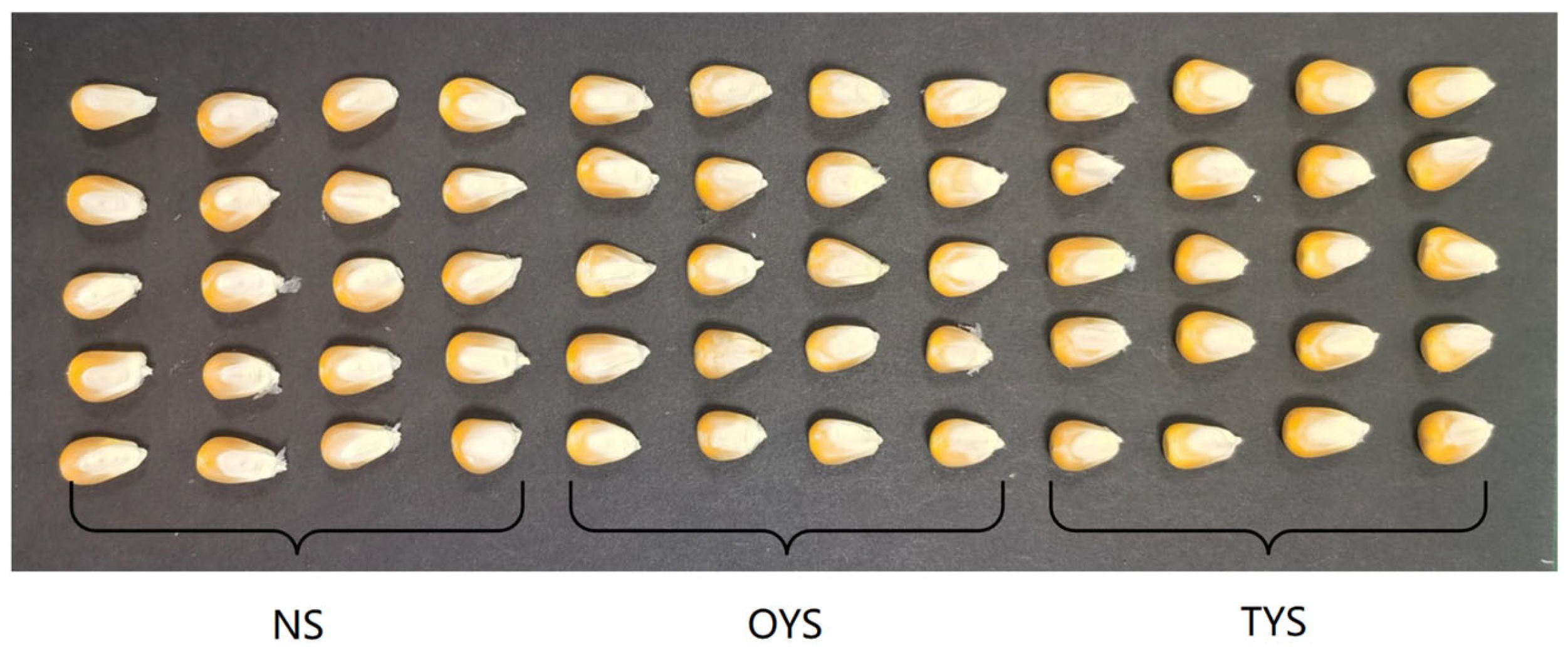
Three different storage periods of maize seeds with similar shapes and sizes were prepared, including new seeds, one-year aged seeds and two years aged seeds, with 300 seeds per storage period as samples. All samples were provided by the Beijing Academy of Agricultural and Forestry Sciences (China). The samples of the three different storage periods are shown in Figure 1. In Figure 1 and subsequent sections of this paper, TYS, OYS, and NS represent two-year aged seeds, one-year aged seeds, and new seeds, respectively.

2.2. Hyperspectral Imaging System

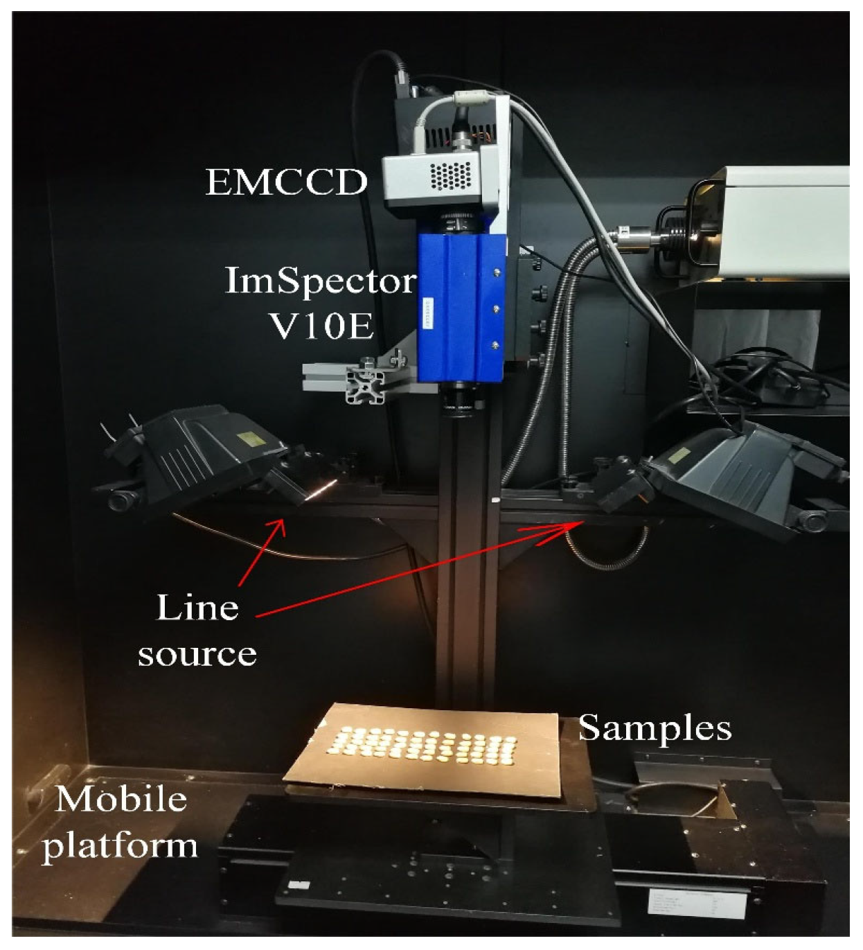
A hyperspectral imaging system which was assembled by ourselves was used to acquire the hyperspectral images of all samples, as shown in Figure 2. The entire system consisted of a 14-bit Vis-NIR electron multiplying charge-coupled device (EMCCD) camera (Andor Luca EMCCD DL-604 M, Andor Technology plc., Belfast, Northern Ireland, UK), a spectrograph with 0.772 nm average resolution (actual resolution varies with wavelength) over a wavelength range of 326.7–1098.1 nm, a 150 W halogen lamp with two line lighting fibers (3900-ER, Illumination Technologies, Inc., Onondaga County, NY, USA), an electronically controlled mobile platform (EZHR17EN, AllMotion, Inc., Union City, CA, USA) and a computer (Dell, Intel (R) Core (TM) i5-2400 CPU @ 3.10 GHZ, Dell Technologies Inc., Round Rock, TX, USA) used for controlling the entire system.

The distance between the lens of the spectrograph and sample stage was set at 380 mm and two line sources were mounted at 45° angles from the horizontal to acquire high-quality hyperspectral images. The movement speed of the sample platform was set at 0.7 mm/s and the exposure time of the camera was 2 ms. Considering the different surface characteristics of both sides of maize seeds, the spectral collection was performed on all samples with the embryo side facing up. A total of 60 samples (20 samples per age group) were placed on a black board and arranged in 5 rows and 12 columns for spectral collection each time. In this way, one complete hyperspectral image collection of all 900 samples was completed after 15 scans. To ensure the representativeness of the acquired hyperspectral data, each individual sample was scanned three times, and the average spectrum extracted from the three hyperspectral images of each sample was used for subsequent analysis.

Before being used for subsequent data processing, the raw hyperspectral image ($R$) must be calibrated to eliminate the influence of non-uniform illumination and variations in the pixel-to-pixel sensitivity of the detector [21,22]. A standard whiteboard was placed in a suitable position on the sample table to obtain the white reference ($W$). With the lens completely covered by a cap and the lamps turned off, the dark reference ($D$) was obtained. The calibrated hyperspectral image ($Y$) was then calculated in accordance with Equation (1):

$$Y={\displaystyle \frac{R-D}{W-D}}$$

(1)

In this study, we utilized hyperspectral images within the 400–1000 nm range for our analysis and did not employ other near-infrared bands. The primary reasons are as follows:

(1)

Direct Correlation with Seed Aging Indicators: Variation in the storage duration of maize seeds leads to the degradation of key biochemical components (chlorophyll, carotenoids, phenolic compounds) and the oxidation of lipids and proteins. These chemical changes are reflected in alterations of the seeds’ optical properties within this specific spectral region.

(2)

Cost and Simplicity: Hyperspectral imaging systems operating in the 400–1000 nm range are generally more cost-effective and easier to implement than NIR systems that require cooled, expensive InGaAs detectors. This cost advantage enables higher-throughput configurations for scalability, making them more suitable for future large-scale applications.

(3)

Spatial Resolution: The shorter wavelengths in the 400–1000 nm range enable higher spatial resolution for imaging fine morphological structures of the seed (e.g., embryo vs. coat), which is essential for the region of interest analysis we performed. This complements the spectral information.

In summary, our choice of the 400–1000 nm range is justified by its direct sensitivity to the key photochemical indicators of seed aging, its practical advantages for high-resolution imaging and potential field deployment.

2.3. Spectra Data Extraction

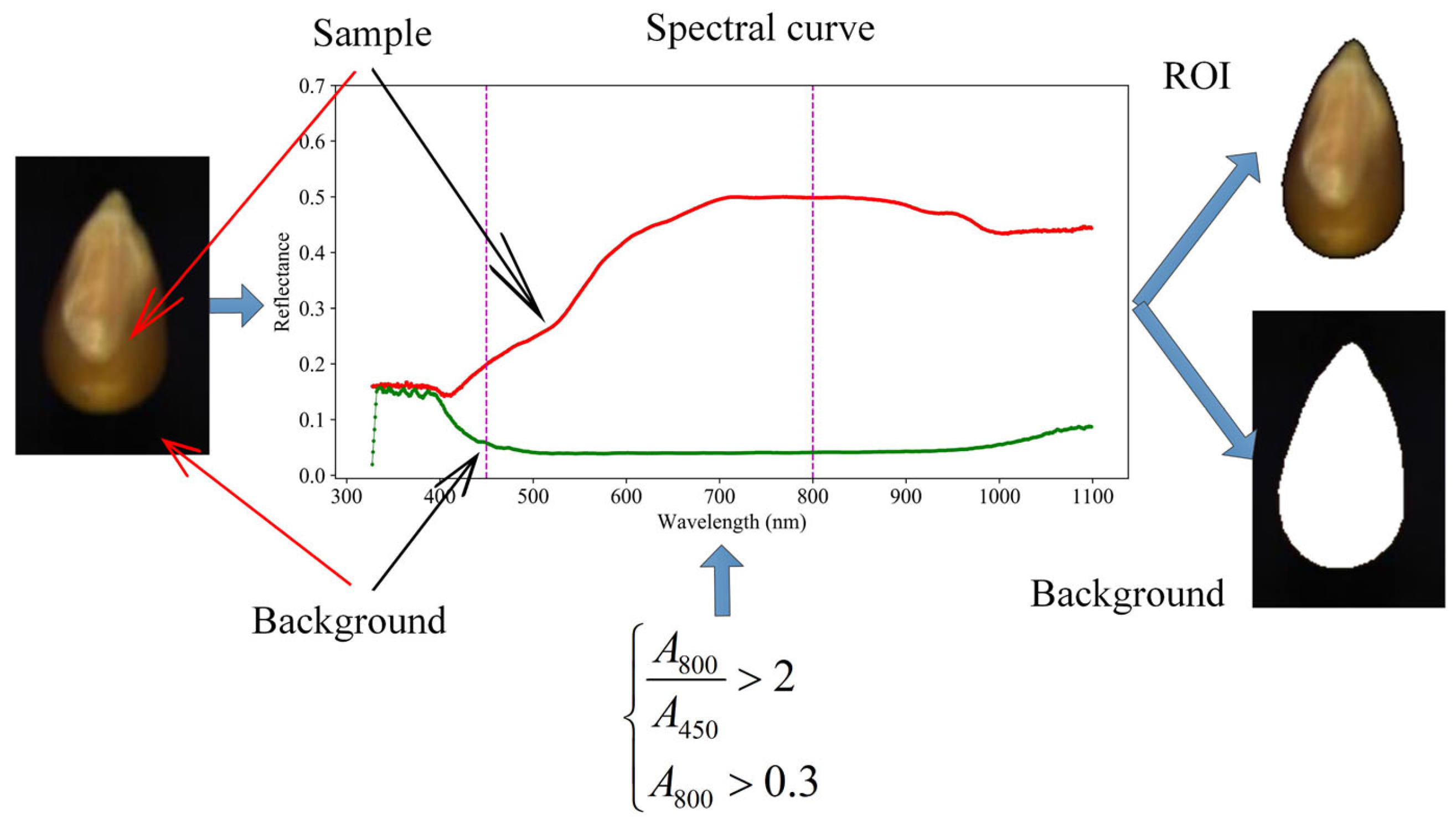
In order to establish a classification model for maize seeds of different ages, the region of interest (ROI) of sample must be determined. In this study, the region of whole seed of the sample was taken as the ROI first. Analysis showed that the spectral intensity of the seed region and the background region was low in the vicinity of 400 nm. The spectral intensity of the seed region reaches a high value around 800 nm, which is over twice as high as that at 400 nm. By contrast, the spectral intensity of the background region was generally less than 0.3 and was comparable to that around 400 nm. Therefore, the spectral intensities at 400 and 800 nm were used to extract spectral data of the ROI. $A400$ and $A800$ were used to represent the spectral intensity at 400 nm and 800 nm, respectively. For any pixel in the image region, when the $A800/A400$ > 2 and $A800$ > 0.3, it was considered as the seed region; otherwise, it is considered as the background region [23]. After segmentation, some of the seed edge regions were removed using morphological filtering and the effective seed regions were retained as the ROI in this study. Then the spectra in each ROI was averaged at each wavelength to reduce the amount of data. The schematic diagram of ROI extraction is shown in Figure 3. In the figure, the red line represents the spectrum of the seed region, and the green line represents the spectrum of the background region.

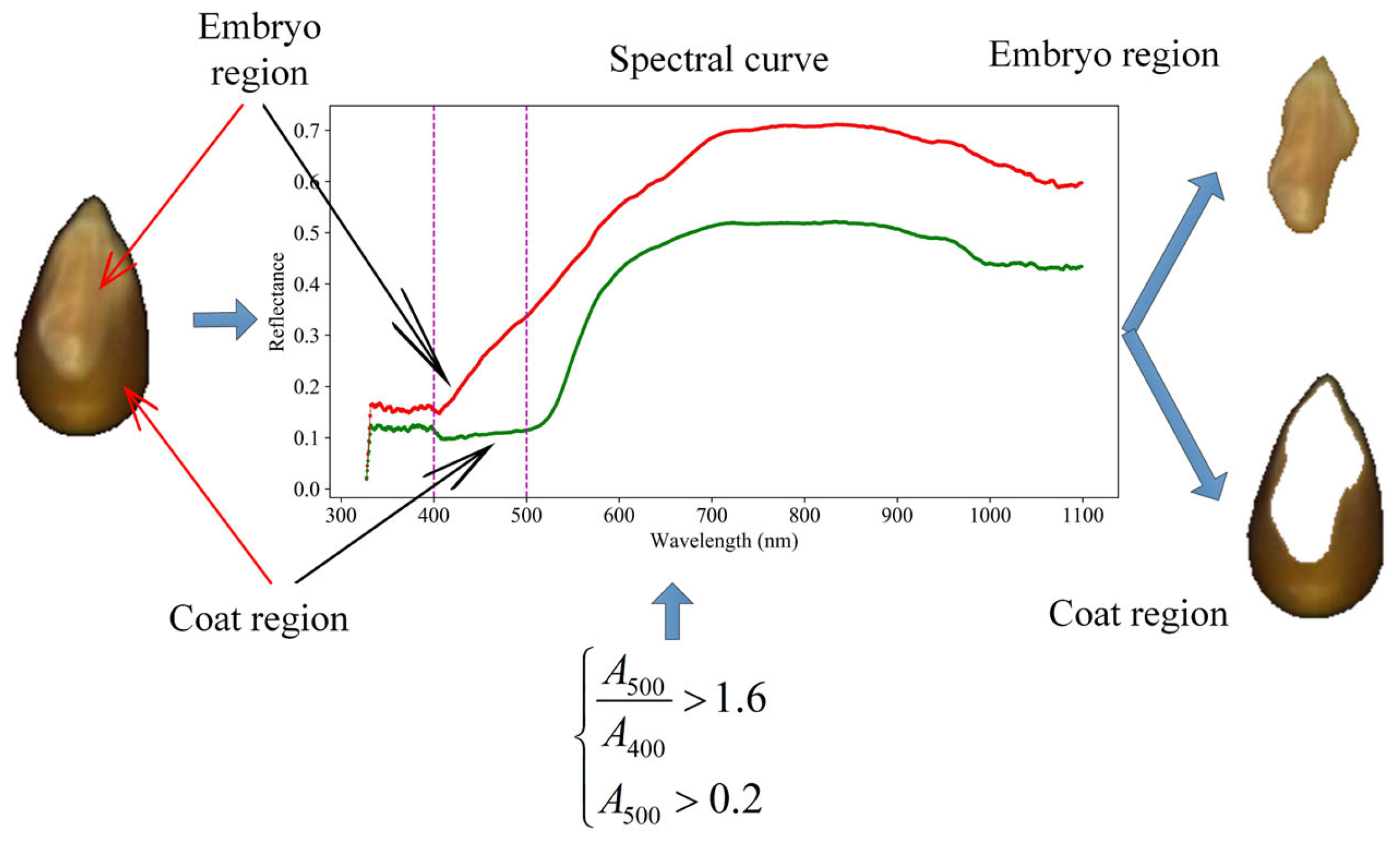
Some studies on maize seeds have shown that the spectrum in the ROI of embryo region for modelling can also yield good results [24]. In this study, on the basis of the ROI of the whole seed region, the ROI of the embryo region was further extracted for study and comparison with the ROI of the whole seed. The specific method is as follows: By observing the spectrum of the embryo region and the coat region of seed, it is found that in the range of 400–500 nm, the spectrum intensity of embryo region shows a trend of increasing with the increase in wavelength, around 500 nm, the spectrum intensity is generally more than twice that at 400 nm, and the spectral intensity is generally greater than 0.2. However, for the coat region, there is no obvious difference between the spectral intensity near 500 nm and 400 nm. $A400$ was used to represent the spectral intensity at 400 nm and $A500$ was the spectral intensity at 500 nm. Preliminary tests showed that a strict threshold of $A500/A400$ > 2 led to the misclassification of some embryonic areas as seed coat. Therefore, a threshold of $A500/A400$ > 1.6 was selected to ensure more robust and complete embryo segmentation. Accordingly, for each pixel of the ROI, when the value of $A500/A400$ > 1.6 and $A500$ > 0.2, it is considered as embryo region, otherwise it is coat region. After segmentation, a small part of the coat region was mistakenly divided into embryo region. Morphological filtering was used to remove this part of the region and retain the effective embryo region. The schematic diagram of embryo region extraction is shown in Figure 4. In the figure, the red line represents the spectrum of the embryo region, and the green line represents the spectrum of the coat region.

2.4. Data Preprocessing

To reduce the influence of some disturbances, such as scattering noise and external stray light in hyperspectral data, the raw spectrum must be preprocessed before further analysis. Savitzky–Golay (SG) smoothing is a commonly used spectral smoothing algorithm, which can eliminate overlapping peaks and reduce the noise interference in the spectrum [25]. The first-order derivative (FD) is helpful to remove baseline shifts and superposed peaks, and can highlight the difference of spectral change trend [26,27]. SG and FD were used to preprocess the raw spectra in this study.

2.5. Key Wavelength Selection Algorithms

2.5.1. Successive Projections Algorithm (SPA) and Random Forest (RF)

SPA is an effective algorithm for selecting hyperspectral key variables. This algorithm uses a simple projection operation in a vector space to select the subsets of variables with a minimum of collinearity, and the candidate variables have the maximum projection value on the orthogonal subspace of the previously selected variables. This algorithm minimizes the variable collinearity and reduces the number of modeling variables without significant loss of predictive power [28,29].

RF is a commonly used algorithm to select the key wavelengths of hyperspectral images. The idea of RF is to calculate the weight of each variable by simulating a Markov chain that obeys a steady-state distribution in the model space. The more important a variable is to the model, the greater the probability that it will be selected. This algorithm integrates the advantages of genetic algorithm and particle swarm optimization algorithm and has the advantages of fast calculation speed, low number of adjustment parameters, and satisfactory global search ability [30,31].

2.5.2. Inter-Class Feature Differences (IFD)

Due to the difference of the distribution range of spectral intensity at different wavelengths, the distribution range of spectral intensity should be unified to the same scale before performing IFD to select characteristic wavelengths, that is, the spectral intensity should be normalized for each wavelength, as shown in Equation (2).

$$x_{w-i}={\displaystyle \frac{x_{w-i\left(org\right)}-x_{w\left(min\right)}}{x_{w\left(max\right)}-x_{w\left(min\right)}}}$$

(2)

where $x_{w-i\left(org\right)}$ represents the original spectral intensity of the sample $i$ at wavelength $w$, $x_{w-i}$ represents the normalized spectral intensity at wavelength $w$, $x_{w\left(max\right)}$ and $x_{w\left(min\right)}$ represent the maximum and minimum spectral intensities at wavelength $w$, respectively. In addition, according to the Kolmogorov–Smirnov (K-S) test, the spectral intensity values of samples in the same year group at all wavelengths basically conform to a normal distribution, so the algorithm proposed in this study is feasible.

For each wavelength $w$, the intra-class mean values of the three classes at that wavelength were calculated. As shown in Equation (3), the $X_{w-v}$ represents the spectral mean value in class $v$ at wavelength $w$.

$$X_{w-v}={\displaystyle \frac{\sum _{i=1}^n{x}_i}{n}}$$

(3)

where $n$ is the number of samples in class $v$. The inter-class mean value at this wavelength is calculated according to Equation (4).

$$X_w={\displaystyle \frac{\sum _{v=1}^m{X}_{w-v}}{m}}$$

(4)

where $X_w$ represents the spectral mean value of inter-class at wavelength $w$, $m$ is the number of classes. The $D_{w-v}$ represents the intra-class variance of class $v$ at wavelength $w$ and $D_w$ represents the inter-class variance of different classes at wavelength $w$, as shown in Equations (5) and (6).

$$D_{w-v}={\displaystyle \frac{\sum _{i=1}^n{\left({x_i-X}_{w-v}\right)}^2}{n}}$$

(5)

$$D_w={\displaystyle \frac{\sum _{v=1}^m{(X_{w-v}-X_w)}^2}{m}}$$

(6)

$S_{w-ab\left(org\right)}$ represents the original eigenvalue of difference between group $a$ and group $b$ at wavelength $w$, which is calculated as Equation (7).

$$S_{w-ab\left(org\right)}={\displaystyle \frac{{2D}_{w-ab}}{D_{w-a}+D_{w-b}}}$$

(7)

where $D_{w-ab}$ represents the inter class variance of group $a$ and group $b$ at wavelength $w$, which is calculated as Equation (8).

$$D_{w-ab}={\displaystyle \frac{{(X_{w-a}-X_{w-ab})}^2+{(X_{w-b}-X_{w-ab})}^2}{2}}$$

(8)

where $X_{w-ab}$ represents the spectral mean value of groups $a$ and $b$ at wavelength $w$.

If the intra-class variance of a certain class was smaller, then the spectral value in this class was denser under this wavelength, which was conducive to classification. In this case, the coefficient value should be increased. Conversely, if the intra-class variance of a certain class was larger, then the distribution of spectral value in this class was sparse under this wavelength, which was not conducive to classification. In this case, the coefficient value should be reduced. Therefore, the coefficient $k$ was expressed as the reciprocal of the intra-class variance of this class, as shown in Equations (9) and (10).

$$k_{w-a}={\displaystyle \frac{1}{D_{w-a}}}$$

(9)

$$k_{w-b}={\displaystyle \frac{1}{D_{w-b}}}$$

(10)

According to Equation (7) and combined with the weighting coefficients of Equations (9) and (10), the eigenvalues of spectral difference between group $a$ and group $b$ at wavelength $w$ can be obtained. To distinguish it from the final IFD algorithm, the calculation is denoted by IFDa and the eigenvalues under this algorithm are denoted by $S_{w-ab}$, as shown in Equation (11).

$$S_{w-ab}={\displaystyle \frac{k_{w-a}{(X_{w-a}-X_{w-ab})}^2+k_{w-b}{(X_{w-b}-X_{w-ab})}^2}{D_{w-a}+D_{w-b}}}$$

(11)

Obviously, the larger the value of $S_{w-ab}$ indicates that the spectral difference of the two groups at that wavelength is greater, which means the wavelength contains important information for the classification of classes $a$ and $b$. Conversely, the smaller the value of $S_{w-ab}$ indicates that the spectral variability of the two groups of samples at that wavelength is smaller, which means the wavelength is less useful for the classification of classes $a$ and $b$.

On the basis of the calculated IFDa values between the two groups of samples, in order to calculate the difference between a certain group and other groups, $S_{w-a}$ was used to represent the difference eigenvalue between group $a$ and other groups, that is, the IFD eigenvalues of group $a$, which can be calculated as Equation (12). The maximum calculated eigenvalue $S_{w-a}$ is considered as the most critical wavelength to distinguish group $a$ from other groups.

$$S_{w-a}=\prod _{b=1}^{m(b\ne a)}{S}_{w-ab}$$

(12)

2.6. Model Construction

The basic idea of linear discriminant analysis (LDA) is to project the high-dimensional data into the optimal discriminant vector space, compress the dimension of the feature space and extract the classification information. The projected samples are guaranteed to have the best separability in the new vector space. LDA can not only be used for dimensionality reduction of data, but also for the establishment of a classification model [32,33]. This study employed the LDA algorithm to develop a classification model for maize seeds with different storage ages.

Since hyperspectral image acquisition for all 900 samples was completed after 15 scanning sessions, and to minimize the impact of different acquisition batches on sample spectra, the samples from 10 randomly selected scanning sessions were designated as the calibration set, with the remaining 5 sessions serving as the prediction set. This allocation resulted in each age group containing 200 calibration samples and 100 prediction samples.

In this study, all data processing and analysis were conducted using the following software tools: Hyperspectral image correction was performed using the Environment for Visualizing Images (ENVI 5.6) software (Harris Geospatial Solutions, Boulder, CO, USA). Spectral data extraction, preprocessing, classification model development, validation, and statistical analysis were performed using Python 3.8.2 (Python Software Foundation, Wilmington, DE, USA) and MATLAB R2021b (The MathWorks, Inc., Natick, MA, USA).

3. Results and Discussion

3.1. Spectral Pretreatment

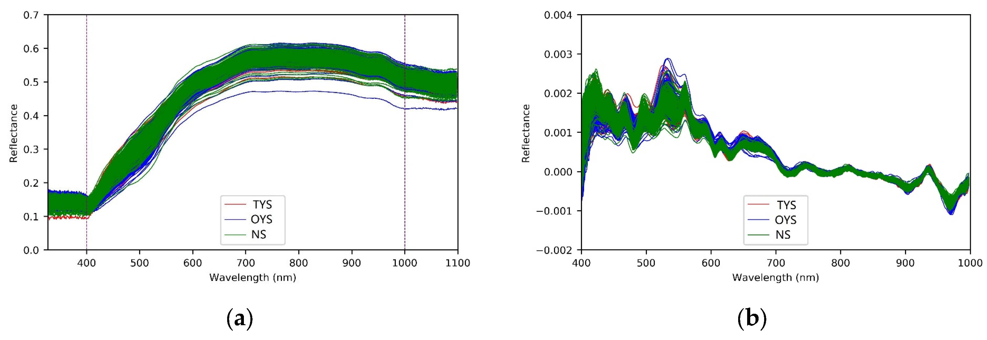
Using the whole seed region as the ROI, the original spectra and SG–FD preprocessed spectra of the calibration set samples are shown in Figure 5. As shown in Figure 5a, the raw spectral data exhibited significant instability and attenuation at wavelengths below 400 nm and above 1000 nm. This is primarily attributed to the combined effects of low instrumental sensitivity (e.g., decreased detector response and light source output at the spectral edges) and experimental artifacts such as uneven illumination on the three-dimensional seed surfaces. Consequently, to ensure the reliability of subsequent analysis, the spectra in these two regions were removed, and 773 wavelengths from 400 to 1000 nm were retained as valid spectra. As noise interference still existed in the retained spectra, SG smoothing was then used to eliminate the effects of these interferences. In order to highlight the spectral differences among samples from different years, the smoothed spectra were further processed by the FD algorithm, resulting in the refined dataset comprising 772 wavelength variables for subsequent analysis (Figure 5b).

To evaluate the impact of spectral preprocessing methods on the classification of different age groups, classification models were developed using an LDA classifier based on raw spectra, noise removed spectra, SG preprocessed spectra, and SG–FD preprocessed spectra. The classification results for the prediction set are shown in

Table 1. Comparison of the effect of raw and preprocessed spectra.

Spectra	Different Aged Samples	Predicted Results				Overall Accuracy
		TYS	OYS	NS	Accuracy
Raw spectra	TYS	81	15	4	81%	81.33%
	OYS	18	77	5	77%
	NS	2	12	86	86%
Spectra with ends removed	TYS	86	12	2	86%	86.33%
	OYS	12	83	5	83%
	NS	1	9	90	90%
SG-smoothed spectra	TYS	90	9	1	90%	89.67%
	OYS	11	85	4	85%
	NS	1	5	94	94%
SG-FD-preprocessed spectra	TYS	93	7	0	93%
	OYS	8	88	4	88%	92.00%
	NS	0	5	95	95%

. As can be seen from Table 1, SG–FD preprocessing outperformed the raw spectra and other preprocessing methods. Consequently, the SG–FD preprocessed spectra were used for the subsequent analysis in this study.

3.2. Key Wavelength Selection

3.2.1. Key Wavelength Selection Based on IFDa

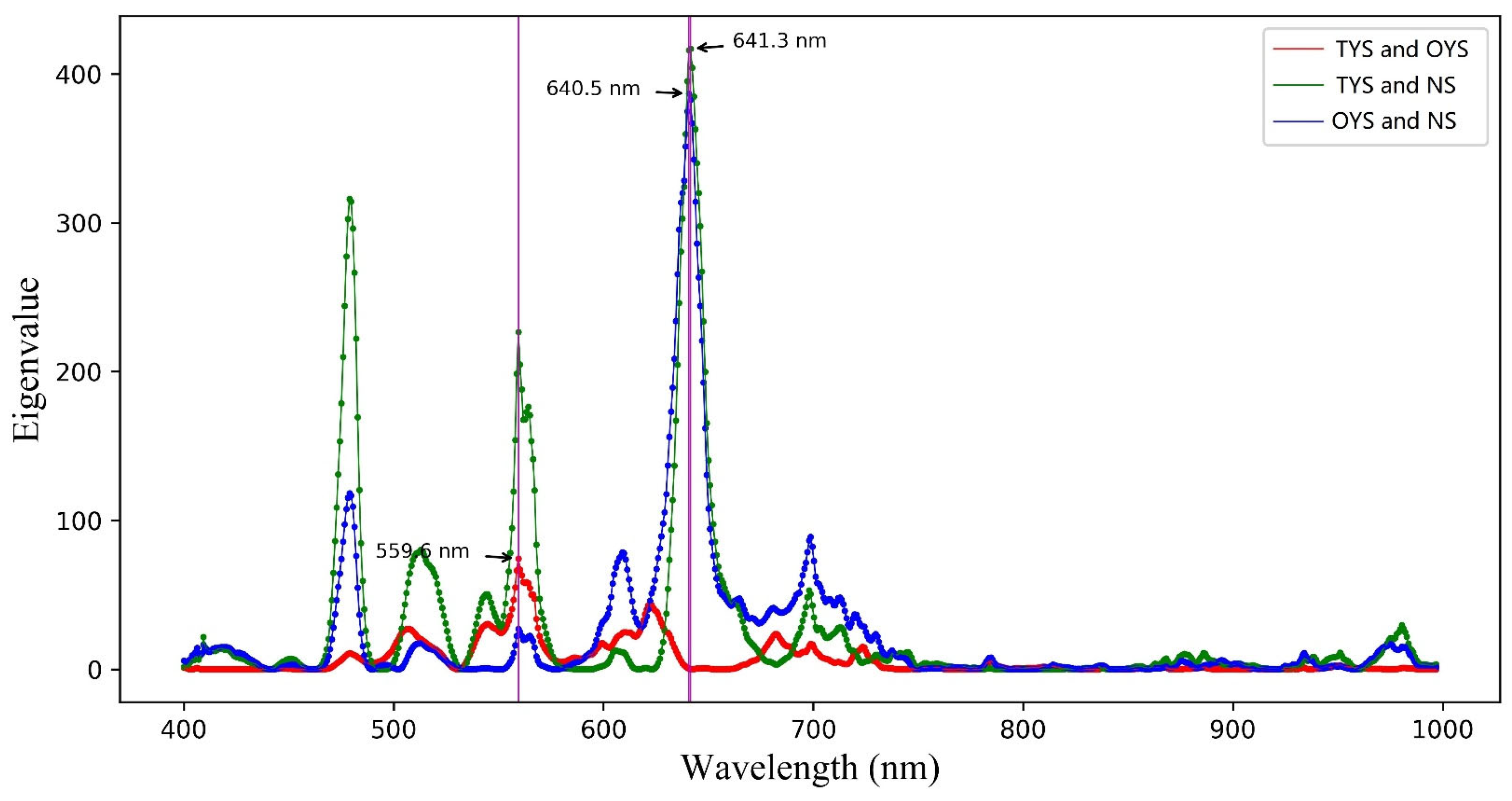
Figure 6 shows the eigenvalues of spectral difference between samples from any two different ages. The red solid line in the figure shows the spectral difference between samples TYS and OYS, the green line shows the spectral difference of samples between TYS and NS, and the blue line shows the spectral difference of samples between OYS and NS. The eigenvalue of spectral difference between TYS and OYS reaches its peak at 559.6 nm, indicating that this wavelength is the key wavelength to distinguish samples from TYS and OYS. Similarly, the blue and green curves peak at adjacent data points, 640.5 nm and 641.3 nm, respectively, which indicates that the spectral region near 641 nm contains critical information for differentiating OYS and TYS from NS samples.

The three wavelengths selected in Figure 6 are considered the most critical for distinguishing maize seeds from any two different ages. Furthermore, it can be observed that both the green and blue curves also peak in the vicinity of 559.6 nm. This indicates that this wavelength simultaneously contains important information for differentiating both OYS from NS and TYS from NS. Therefore, these three wavelengths are the key wavelengths selected based on the IFDa algorithm in this study.

3.2.2. Key Wavelength Selection Based on IFD

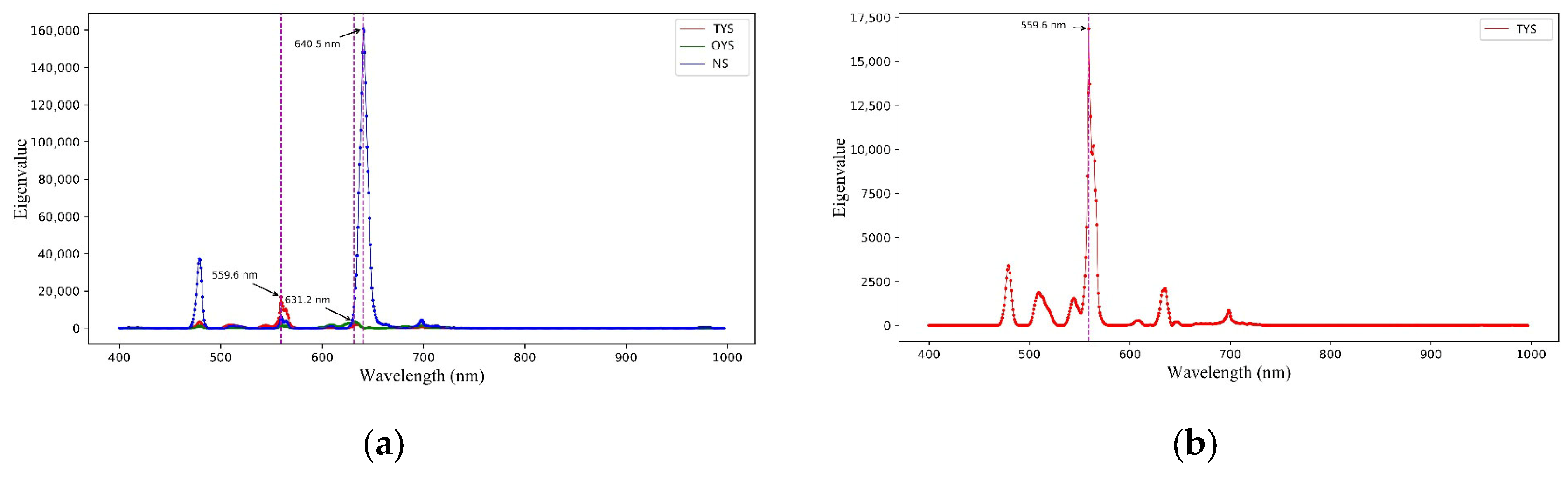
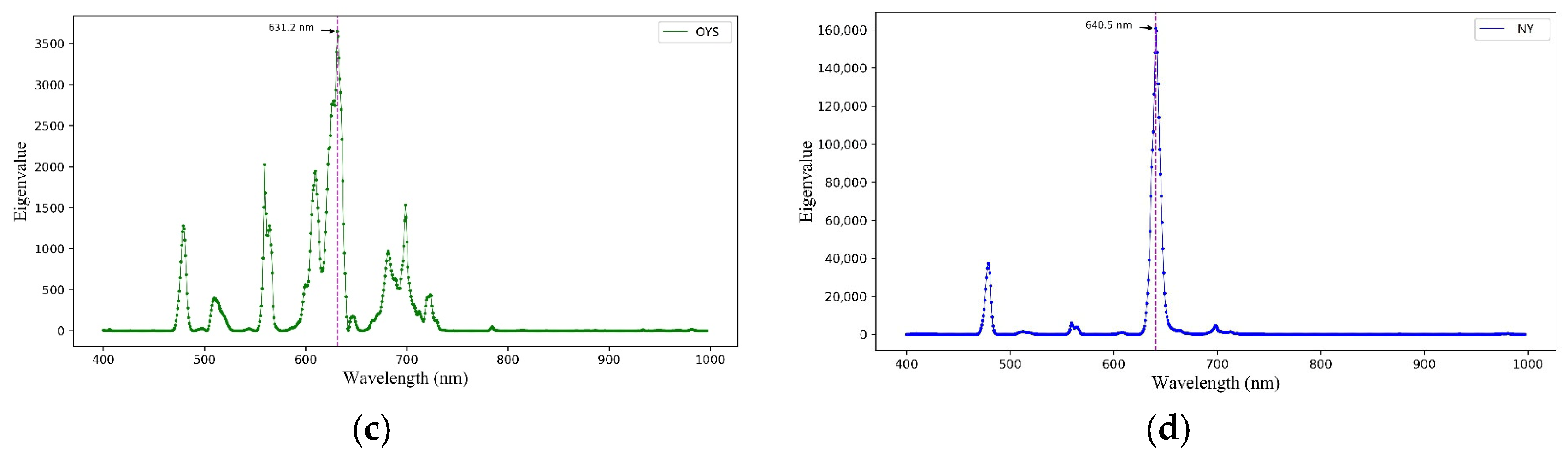
After calculating the eigenvalues of the spectral differences between any two different ages based on IFDa, Equation (12) was further used to compute the eigenvalues of the spectral differences between any given age and the other ages. The results are shown in Figure 7. In the figure, the red, green, and blue lines represent the spectral difference eigenvalues for TYS, OYS, and NS against the other ages, respectively. It can be observed that the red, green, and blue lines reach their maximum values at 559.6 nm, 631.2 nm, and 640.5 nm, respectively (the data for the selected wavelengths are provided in the Supplementary Materials, and Data S1 and Data S2 are the calibration data and prediction data, respectively). This indicates that these three wavelengths contain the most critical information for identifying samples from these three distinct ages. Furthermore, the results demonstrate that compared to the wavelengths selected by IFDa, only one wavelength differs in this set, while the other two remain consistent.

The selected three key wavelengths are distributed within the 550–650 nm range. Although this range does not contain the primary absorption features of starch or water, it captures critical information related to pigment degradation—an early hallmark of seed senescence. This physiological state co-occurs with the deterioration of major components like starch and the loss of moisture [34].

3.3. Discrimination Results for Samples of Different Ages

Discrimination models were developed using LDA based on the three key wavelengths selected by IFDa and IFD, as well as on the full wavelengths. The test results are presented in

Table 2. Discrimination results of samples under full wavelength and key wavelength.

Number of Bands	Different Aged Samples	Predicted Results				Overall Accuracy
		TYS	OYS	NS	Accuracy
772 bands	TYS	93	7	0	93%	92.00%
	OYS	8	88	4	88%
	NS	0	5	95	95%
3 key wavelengths selected by IFD (559.6, 631.2 and 640.5 nm)	TYS	82	18	0	82%	85.67%
	OYS	11	81	8	81%
	NS	0	6	94	94%
3 key wavelengths selected by IFDa (559.6, 640.5 and 641.3 nm)	TYS	84	16	0	84%	85.00%
	OYS	14	77	9	77%
	NS	1	5	94	94%

. It can be observed that with the full wavelengths, the discriminant accuracy for the prediction set reached 93.00%. When only the three key wavelengths selected by IFDa and IFD were used, the discrimination accuracies for the prediction set were 85.00% and 85.67%, respectively, which are only slightly lower than that achieved with the full wavelengths. Since the wavelengths selected by IFD take into account the differences between each age samples and all other different-aged groups, whereas IFDa only considers the differences between any two specific different-aged groups, the discrimination result based on IFD is slightly superior to that based on IFDa when using the same number of wavelengths.

As can be seen from Table 2, when using the three key wavelengths selected by IFD, the identification accuracy for NS samples is considerably higher than that for TYS and OYS samples. This finding corresponds with the results shown in Figure 6, where the IFD eigenvalue for NS samples is significantly higher than those for TYS and OYS. Consequently, the identification of NS achieved superior results.

The results in Table 2 also indicate that most misclassified samples from TYS were assigned to OYS, and likewise, most misclassified samples from OYS were assigned to TYS. The primary cause of the high mutual misclassification rate between OYS and TYS and the high accuracy for NS lies in the relative magnitude of chemical differences. The chemical composition of maize undergoes drastic alterations during the initial transition from freshness to storage, involving rapid degradation of pigments, significant moisture loss, and the onset of lipid oxidation. These changes create a substantial compositional gap between fresh and stored kernels. In contrast, the chemical difference between OYS and TYS is incremental, representing only further progression of the same degradation processes. This difference is even smaller than the inherent compositional variability between some individual samples. Consequently, most errors arise from the mutual misclassification between OYS and TYS.

3.4. Comparison of ROIs for Whole Seed and Embryo

Based on the spectral data of the whole seed region, a satisfactory result was achieved for detecting aged maize seeds. In order to evaluate the effect of the ROI on the model performance, the spectra extracted from the embryo region were compared with those from the whole seed region.

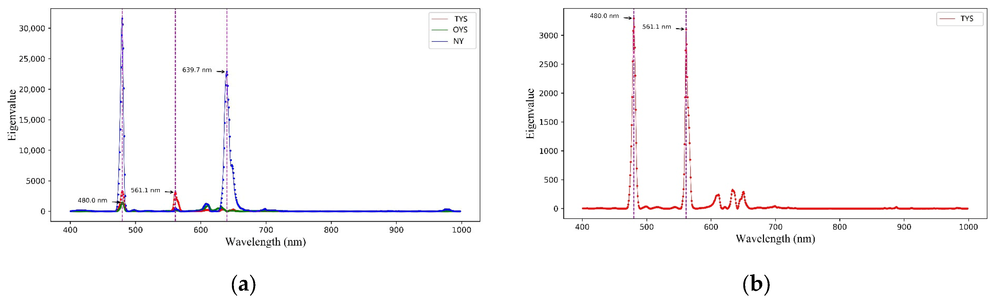
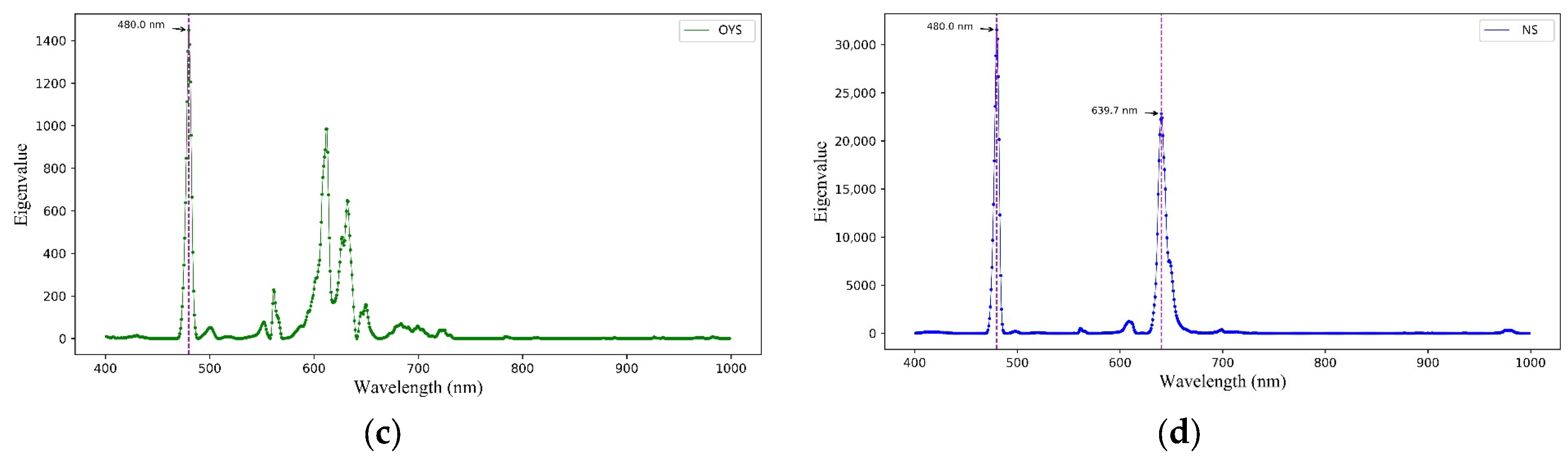
Using the seed embryo region as the ROI, the IFD eigenvalues for samples from the three different age groups were calculated to select key wavelengths; the results are shown in Figure 8. The results indicate that the most significant wavelength selected for classifying all three different ages is 480.0 nm, suggesting that this wavelength has a substantial influence on discriminating the samples from these three age groups.

To compare the identification results with those based on the three wavelengths selected from the whole seed region, the curves in Figure 8 were examined. For TYS, the IFD eigenvalue at 561.1 nm is slightly lower than that at 480.0 nm. Similarly, for NS, the IFD eigenvalue at 639.7 nm is also close to that at 480.0 nm. For OYS, however, the IFD eigenvalue at 480.0 nm is considerably higher than those at other wavelengths. Therefore, for the embryo region as the ROI, the wavelengths 480.0 nm, 561.1 nm, and 639.7 nm were selected as the three key wavelengths under the IFD algorithm.

Table 3. Comparison of the results of two different ROIs.

Different ROI of Samples	Different Aged Samples	Predicted Results				Overall Accuracy
		TYS	OYS	NS	Accuracy
Whole seed region	TYS	82	18	0	82%	85.67%
	OYS	11	81	8	81%
	NS	0	6	94	94%
Embryo region	TYS	82	17	1	82%	84.33%
	OYS	13	78	9	78%
	NS	1	6	93	93%

presents the sample discrimination results under the two different ROIs: the whole seed region and the embryo region. It can be observed that the discriminant performance based on the whole seed region is slightly superior to that achieved using only the embryo region. The reason for this is likely that the whole seed region includes not only the embryo, but also the seed coat region, and the spectral information from the seed coat also contributes to age discrimination, thereby providing more comprehensive information than using the embryo alone.

3.5. Comparison with Other Key Wavelength Selection Algorithms

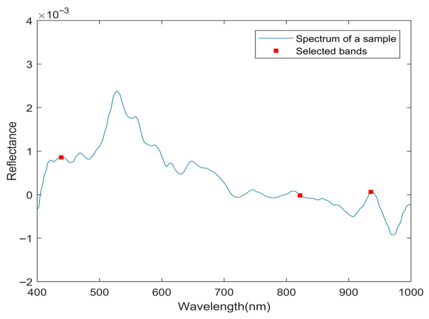
To validate the effectiveness of the key wavelength selection algorithm proposed in this study, a comparative analysis was conducted against two classical variable selection algorithms, SPA and RF, each used to select three key wavelengths. For SPA, key wavelengths were selected based on the optimal combination principle, with the number of characteristic variables and the number of fold cross-validation set to 3 and 10, respectively. Finally, three wavelengths at 436.7, 818.6 and 935.1 nm were selected as key wavelengths, as shown in Figure 9.

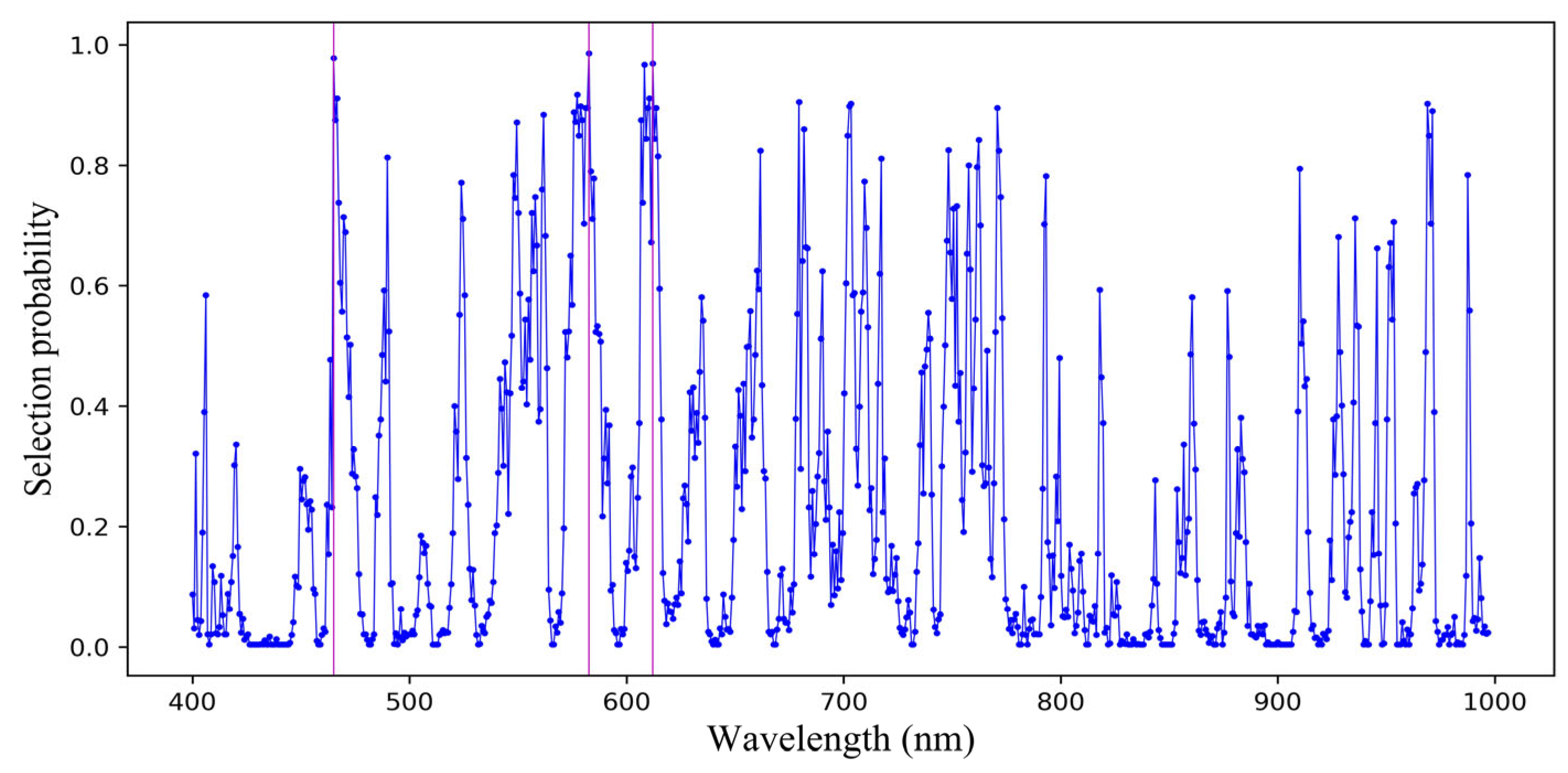
Before running the RF algorithm, the number of simulations and the maximum number of latent variables for cross-validation were set to 10,000 and 3, respectively. Using the RF algorithm, the selection probability for each wavelength was calculated; a higher probability indicates greater importance of the wavelength. Figure 10 shows the calculated selection probability for each wavelength and the three key wavelengths with the largest probabilities (462.8, 582.6, and 611.8 nm) were selected.

The comparison results based on different wavelength selection methods are shown in

Table 4. Discrimination results of samples with different key wavelength selection algorithms.

Different Wavelength Selection Methods	Different Aged Samples	Predicted Results				Overall Accuracy
		TYS	OYS	NS	Accuracy
Proposed method	TYS	82	18	0	82%	85.67%
	OYS	11	81	8	81%
	NS	0	6	94	94%
SPA	TYS	40	48	12	40%	52.33%
	OYS	19	44	37	44%
	NS	14	13	73	73%
RF	TYS	40	30	30	40%	54.67%
	OYS	38	51	11	51%
	NS	19	8	73	73%

. The IFD algorithm proposed in this study achieved the best result when only three key wavelengths were used. This is because the algorithm quantifies the difference features between classes, and has certain advantages when only a few key wavelengths are extracted.

The results demonstrate that with only three wavelengths, the algorithm proposed in this study significantly outperforms both SPA and RF. In this study, the performance of both SPA and RF was suboptimal when only three key wavelengths were selected. This may be attributed to the fact that SPA relies on linear combinations of specific wavelengths, which limits its ability to capture complex, non-linear variations in spectral features. The RF algorithm relies on a stochastic, iterative process to evaluate numerous wavelength combinations. When the target subset size is extremely small, the probability of its random search converging to an optimal, stable, and discriminative minimal set within limited iterations is significantly reduced.

In contrast, the higher discrimination accuracy achieved by our proposed IFD method can likely be attributed to its mechanism of selecting key wavelengths based on spectral feature differences. By identifying and utilizing the spectral bands that exhibit the greatest inter-class variance, IFD is able to deliver relatively favorable performance even with a limited number of wavelengths.

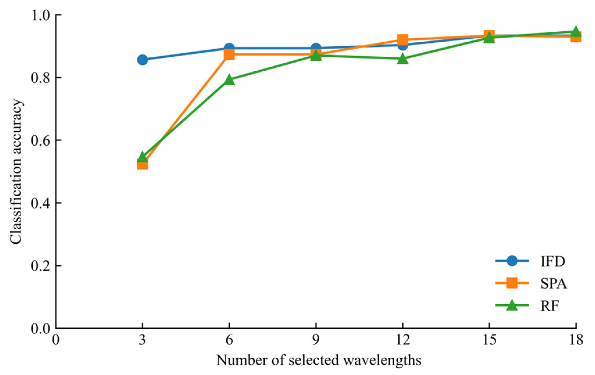
As the number of selected key wavelengths increases, the performance of the IFD, SPA, and RF methods, all implemented based on the LDA model, is shown in Figure 11. (Note: Because IFD selects an equal number of wavelengths from each group based on spectral differences among groups, the numbers of wavelengths shown are integer multiples of 3).

As shown in Figure 11, when the number of key wavelengths selected by these three algorithms increases, the model performance improves accordingly. When the number of selected key wavelengths reaches 15, the test accuracy of the prediction set for all methods exceeds 90%. As the number of selected key wavelengths continues to increase, the discriminant results of SPA and RF gradually catch up with or surpass the IFD algorithm proposed in this study. The reason lies in the fact that the IFD algorithm proposed in this study selects key wavelengths based on the spectral difference features between each sample group and other groups. When a small number of wavelengths is selected (e.g., 3), the chosen wavelengths represent those with the greatest differences between each group and the others. However, further increasing the number of selected wavelengths introduces a certain degree of information redundancy, leading to a slower improvement in model performance. When the number of key wavelengths reaches a certain threshold, the IFD algorithm no longer maintains an advantage over other algorithms (such as SPA and RF). Nevertheless, the IFD algorithm proposed in this study demonstrates certain advantages when selecting a smaller number of wavelengths.

3.6. Discrimination Results of New and Aged Maize Seeds

To further distinguish between new and aged seeds, the samples from TYS and OYS were merged to form an ‘aged seeds’ (TYS-OYS) group. The LDA model was used to distinguish between new and aged samples based on both the three wavelengths selected by IFD and the full wavelengths, and the discrimination results are shown in

Table 5. Discrimination results of new and aged samples.

Number of Bands	Year of Samples	Predicted Results			Overall Accuracy
		TYS-OYS	NS	Accuracy
772 bands	TYS-OYS	196	4	98.00%	97.00%
	NS	5	95	95.00%
3 key wavelengths	TYS-OYS	192	8	96.00%	95.33%
	NS	6	94	94.00%

.

It can be seen from Table 5 that when using the full wavelength, the discrimination accuracy for the predicted set samples reaches 97.00%. Using only the three key wavelengths selected by IFD, the discrimination accuracy for the predicted set reached 95.33%. The results demonstrate that the proposed algorithm enables the discrimination of maize seeds of different ages, as well as new and aged maize seeds, using a minimal set of key wavelengths.

3.7. Discussion of Key Wavelengths Selected by IFD

The key wavelengths identified in this study align closely with feature bands reported in prior studies on grain and seed quality. In the study by Guo et al. [35] on soybean moisture content, where 14 feature bands were selected using SPA within 400–1000 nm, the reported wavelengths of 599 nm and 641 nm are highly consistent with those identified in our study (559.6, and 640.5 nm). Similarly, in the research by Xiong et al. [36] on barley grain hardness, the selected feature wavelength of 630 nm closely matches our finding of 631.2 nm. Given this striking agreement with existing literature, we speculate that these bands collectively constitute a spectral region that is highly sensitive to common deterioration processes—such as water migration and textural hardening—in cereal grains during storage.

4. Conclusions

This study investigated the feasibility of using hyperspectral imaging (400–1000 nm) to discriminate maize seeds of three different storage ages. Based on the hyperspectral data of the whole seed region, after spectral preprocessing, three key wavelengths were selected using the key wavelength selection algorithm proposed in this study. These wavelengths were combined with LDA to construct a discrimination model. The model achieved a discrimination accuracy of 85.67% for discriminating the three age groups and 95.33% for classifying new and aged seeds, demonstrating good identification performance and reflecting the effectiveness of the proposed algorithm.

This study also explored the impact of different preprocessing schemes on the model to identify the optimal one. Furthermore, different ROIs based on the whole seed region and embryo region were studied to explore the impact of different ROIs on the model recognition results and determine the optimal ROI. In summary, a key wavelength selection algorithm for hyperspectral data was developed. The selected wavelengths effectively captured the spectral differences among samples of different ages, enabling high-accuracy identification. The algorithm holds a significant advantage over traditional variable selection methods (e.g., RF and SPA) when only a minimal number of wavelengths are required. Future work will focus on exploring the impact of various aging degrees on the nutritional components of maize and developing corresponding detection methods. In subsequent studies, we will target larger sample sizes to meet more stringent methodological standards.

References

1. Tenaillon, M.I.; Charcosset, A. A European perspective on maize history. Comptes Rendus Biol. 2011, 334, 221–228. [Google Scholar] [CrossRef] [Scilit]
2. Li, L.; Huang, W.; Wang, Z.; Liu, S.; He, X.; Fan, S. Calibration transfer between developed portable Vis/NIR devices for detection of soluble solids contents in apple. Postharvest Biol. Technol. 2022, 183, 111720. [Google Scholar] [CrossRef] [Scilit]
3. Jin, X.; Chen, X.; Shi, C.; Li, M.; Guan, Y.; Yu, C.Y.; Yamada, T.; Sacks, E.J.; Peng, J. Determination of hemicellulose, cellulose and lignin content using visible and near infrared spectroscopy in Miscanthus sinensis. Bioresour. Technol. 2017, 241, 603–609. [Google Scholar] [CrossRef] [Scilit] [PubMed]
4. Huang, M.; Zhao, W.Y.; Wang, Q.G.; Zhang, M.; Zhu, Q.B. Prediction of moisture content uniformity using hyperspectral imaging technology during the drying of maize kernel. Int. Agrophys. 2015, 29, 39–46. [Google Scholar] [CrossRef] [Scilit]
5. Zhang, Y.; Guo, W. Moisture content detection of maize seed based on visible/near-infrared and near-infrared hyperspectral imaging technology. Int. J. Food Sci. 2020, 55, 631–640. [Google Scholar] [CrossRef] [Scilit]
6. Yang, X.L.; You, Z.H.; Cheng, F. Study on Identification of Immature Corn Seed Using Hyperspectral Imaging. Spectrosc. Spect. Anal. 2016, 36, 4028–4033. [Google Scholar]
7. Wang, Z.L.; Tian, X.; Fan, S.X.; Zhang, C.; Li, J.B. Maturity determination of single maize seed by using near-infrared hyperspectral imaging coupled with comparative analysis of multiple classification models. Infrared Phys. Technol. 2021, 112, 103596. [Google Scholar] [CrossRef] [Scilit]
8. Wang, L.; Sun, D.W.; Pu, H.B.; Zhu, Z.W. Application of Hyperspectral Imaging to Discriminate the Variety of Maize Seeds. Food Anal. Methods 2016, 9, 225–234. [Google Scholar] [CrossRef] [Scilit]
9. Zhao, Y.Y.; Zhu, S.S.; Zhang, C.; Feng, X.P.; Feng, L.; He, Y. Application of hyperspectral imaging and chemometrics for variety classification of maize seeds. RSC Adv. 2018, 8, 1337–1345. [Google Scholar] [CrossRef] [Scilit]
10. Huang, M.; Tang, J.Y.; Yang, B.; Zhu, Q.B. Classification of maize seeds of different years based on hyperspectral imaging and model updating. Comput. Electron. Agric. 2016, 122, 139–145. [Google Scholar] [CrossRef] [Scilit]
11. Mendoza, F.; Lu, R.F.; Ariana, D.; Cen, H.Y.; Bailey, B. Integrated spectral and image analysis of hyperspectral scattering data for prediction of apple fruit firmness and soluble solids content. Postharvest Biol. Technol. 2011, 62, 149–160. [Google Scholar] [CrossRef] [Scilit]
12. Gao, Z.; Shao, Y.; Xuan, G.; Wang, Y.; Liu, Y.; Han, X. Real-time hyperspectral imaging for the in-field estimation of strawberry ripeness with deep learning. Artif. Intell. Agric. 2020, 4, 31–38. [Google Scholar] [CrossRef] [Scilit]
13. Dalponte, M.; Bruzzone, L.; Vescovo, L.; Gianelle, D. The role of spectral resolution and classifier complexity in the analysis of hyperspectral images of forest areas. Remote Sens. Environ. 2009, 113, 2345–2355. [Google Scholar] [CrossRef] [Scilit]
14. Mianji, F.A.; Zhang, Y. Robust Hyperspectral Classification Using Relevance Vector Machine. IEEE Trans. Geosci. Remote Sens. 2011, 49, 2100–2112. [Google Scholar] [CrossRef] [Scilit]
15. Liu, D.; Sun, D.W.; Zeng, X.A. Recent Advances in Wavelength Selection Techniques for Hyperspectral Image Processing in the Food Industry. Food Bioprocess Technol. 2014, 7, 307–323. [Google Scholar] [CrossRef] [Scilit]
16. Araújo, M.C.U.; Saldanha, T.C.B.; Galvão, R.K.H.; Yoneyama, T.; Chame, H.C.; Visani, V. The successive projections algorithm for variable selection in spectroscopic multicomponent analysis. Chemom. Intell. Lab. Syst. 2001, 57, 65–73. [Google Scholar] [CrossRef] [Scilit]
17. Pontes, M.J.C.; Galvao, R.K.H.; Araujo, M.C.U.; Nogueira, P.; Moreira, T.; Neto, O.D.P.; Jose, G.E.; Saldanha, T.C.B. The successive projections algorithm for spectral variable selection in classification problems. Chemom. Intell. Lab. Syst. 2005, 78, 11–18. [Google Scholar] [CrossRef] [Scilit]
18. Hu, M.H.; Dong, Q.L.; Liu, B.L.; Opara, U.L.; Chen, L. Estimating blueberry mechanical properties based on random frog selected hyperspectral data. Postharvest Biol. Technol. 2015, 106, 1–10. [Google Scholar] [CrossRef] [Scilit]
19. Lin, C.Y.; Bondell, H.; Hao, H.Z.; Hui, Z. Variable Selection for Nonparametric Quantile Regression via Smoothing Spline AN OVA. Stat 2012, 2, 255–268. [Google Scholar] [CrossRef] [Scilit]
20. Wu, L.C.; Zhang, Z.Z.; Xu, D.K. Variable selection in joint mean and variance models of Box-Cox transformation. J. Appl. Stat. 2012, 39, 2543–2555. [Google Scholar] [CrossRef] [Scilit]
21. Fan, S.X.; Huang, W.Q.; Guo, Z.M.; Zhang, B.H.; Zhao, C.J. Prediction of Soluble Solids Content and Firmness of Pears Using Hyperspectral Reflectance Imaging. Food Anal. Method 2015, 8, 1936–1946. [Google Scholar] [CrossRef] [Scilit]
22. Li, J.B.; Wang, Q.Y.; Xu, L.; Tian, X.; Xia, Y.; Fan, S.X. Comparison and Optimization of Models for Determination of Sugar Content in Pear by Portable Vis-NIR Spectroscopy Coupled with Wavelength Selection Algorithm. Food Anal. Method 2019, 12, 12–22. [Google Scholar] [CrossRef] [Scilit]
23. Zhang, B.H.; Liu, L.S.; Gu, B.X.; Zhou, J.; Huang, J.C.; Tian, G.Z. From hyperspectral imaging to multispectral imaging: Portability and stability of HIS-MIS algorithms for common defect detection. Postharvest Biol. Technol. 2018, 137, 95–105. [Google Scholar] [CrossRef] [Scilit]
24. Tian, X.; Huang, W.Q.; Li, J.B.; Fan, S.X.; Zhang, B.H. Measuring the Moisture Content in Maize Kernel Based on Hyperspctral Image of Embryo Region. Spectrosc. Spect. Anal. 2016, 36, 3237–3242. [Google Scholar]
25. Savitzky, A.; Golay, M. Smoothing and Differentiation of Data by Simplified Least Squares Procedures. Anal. Chem. 1964, 36, 1627–1639. [Google Scholar] [CrossRef] [Scilit]
26. Nicolaï, B.M.; Beullens, K.; Bobelyn, E.; Peirs, A.; Saeys, W.; Theron, K.I.; Lammertyn, J. Nondestructive measurement of fruit and vegetable quality by means of NIR spectroscopy: A review. Postharvest Biol. Technol. 2007, 46, 99–118. [Google Scholar] [CrossRef] [Scilit]
27. Wang, H.L.; Peng, J.Y.; Xie, C.Q.; Bao, Y.D.; He, Y. Fruit Quality Evaluation Using Spectroscopy Technology: A Review. Sensors 2015, 15, 11889–11927. [Google Scholar] [CrossRef] [Scilit]
28. Ye, S.F.; Wang, D.; Min, S.G. Successive projections algorithm combined with uninformative variable elimination for spectral variable selection. Chemom. Intell. Lab. Syst. 2008, 91, 194–199. [Google Scholar] [CrossRef] [Scilit]
29. Soares, S.F.C.; Gomes, A.A.; Galvao, A.R.; Araujo, M.C.U.; Galvao, R.K.H. The successive projections algorithm. Trac-Trends Anal. Chem. 2013, 42, 84–98. [Google Scholar] [CrossRef] [Scilit]
30. Li, X.L.; Sun, C.J.; Luo, L.B.; He, Y. Determination of tea polyphenols content by infrared spectroscopy coupled with iPLS and random frog techniques. Comput. Electron. Agric. 2015, 112, 28–35. [Google Scholar] [CrossRef] [Scilit]
31. Chen, J.Y.; Li, G.H. Prediction of moisture content of wood using Modified Random Frog and Vis-NIR hyperspectral imaging. Infrared Phys. Technol. 2020, 105, 103225. [Google Scholar] [CrossRef] [Scilit]
32. Le, K.T.; Chaux, C.; Richard, F.J.P.; Guedj, E. An adapted linear discriminant analysis with variable selection for the classification in high-dimension, and an application to medical data. Comput. Stat. Data Anal. 2020, 152, 107031. [Google Scholar] [CrossRef] [Scilit]
33. Jiang, Y.C.; Leung, F.H.F. Investigating and improving the utility of probabilistic linear discriminant analysis for acoustic signal classification. Digit. Signal Process. 2021, 114, 103055. [Google Scholar] [CrossRef] [Scilit]
34. Yang, S.; Zhu, Q.B.; Huang, M. Application of Joint Skewness Algorithm to Select Optimal Wavelengths of Hyperspectral Image for Maize Seed Classification. Spectrosc. Spect. Anal. 2017, 37, 990–996. [Google Scholar]
35. Guo, Z.; Zhang, J.; Ma, C.; Yin, X.; Guo, Y.; Sun, X.; Jin, C. Application of visible-near-infrared hyperspectral imaging technology coupled with wavelength selection algorithm for rapid determination of moisture content of soybean seeds. J. Food Compos. Anal. 2023, 116, 105048. [Google Scholar] [CrossRef] [Scilit]
36. Xiong, C.; She, Y.; Jiao, X.; Zhang, T.; Wang, M.; Wang, M.; Abd El-Aty, A.M.; Wang, J.; Xiao, M. Rapid nondestructive hardness detection of black highland barley kernels via hyperspectral imaging. J. Food Compos. Anal. 2024, 127, 11. [Google Scholar] [CrossRef] [Scilit]
Figure 1. Maize seed samples with three storage ages.
Agriculture 16 00196 g001
Figure 2. Hyperspectral image acquisition system.
Agriculture 16 00196 g002
Figure 3. The extraction of ROI region.
Agriculture 16 00196 g003
Figure 4. The extraction of embryo region.
Agriculture 16 00196 g004
Figure 5. Spectra before and after pretreatment. (a) spectra before pretreatment; (b) spectra after pretreatment.
Agriculture 16 00196 g005
Figure 6. IFDa eigenvalues at each wavelength for any two different age groups.
Agriculture 16 00196 g006
Figure 7. The eigenvalues and selected key wavelengths using IFD algorithm. (a) IFD eigenvalues and key wavelengths of three different year groups; (b) IFD eigenvalues and key wavelengths for discrimination between TYS and others; (c) IFD eigenvalues and key wavelengths for discrimination between OYS and others; (d) IFD eigenvalues and key wavelengths for discrimination between NS and others.
Agriculture 16 00196 g007aAgriculture 16 00196 g007b
Figure 8. The eigenvalues and selected key wavelengths based on embryo region using IFD algorithm. (a) IFD eigenvalues and key wavelengths of three different year groups; (b) IFD eigenvalues and key wavelengths for discrimination between TYS and others; (c) IFD eigenvalues and key wavelengths for discrimination between OYS and others; (d) IFD eigenvalues and key wavelengths for discrimination between NS and others.
Agriculture 16 00196 g008aAgriculture 16 00196 g008b
Figure 9. The three selected key wavelengths in SPA.
Agriculture 16 00196 g009
Figure 10. Wavelength selection probability and key wavelengths identified by the RF algorithm.
Agriculture 16 00196 g010
Figure 11. Comparison of different wavelength selection algorithms across 3–18 key wavelengths.
Agriculture 16 00196 g011