Vibration Source Identification and Targeted Vibration Reduction of a Tracked Combine Harvester Cab Based on HGWO-VMD

Abstract

To address excessive cab vibration observed after combine harvester manufacture, this study applies hybrid grey wolf–whale optimized variational mode decomposition (HGWO–VMD) to identify vibration characteristics during stationary no-load operation and evaluates targeted mechanical modifications for vibration reduction. Tests were conducted on a Linhai 4LZ-7A tracked combine harvester with only the engine running (Condition A) and with the engine and working components running (Condition B). HGWO–VMD was compared with conventional VMD using manually specified parameters. The target-frequency energy ratios reached 0.704 under Condition A and 0.821 under Condition B for the analyzed signals. Frequency components were consistent with engine rotation and second-order excitation, vibrating screen and cutter operation, and sixth-order threshing drum excitation. A component at 58.88 Hz was also observed and may be associated with the dynamic response of the cab system. The implemented measures comprised vibrating screen counterweight balancing, cutter speed adjustment and counterweight balancing, and inclined cab supports. Among the tested combinations, the selected scheme reduced the measured overall cab and header acceleration RMS values by 48.33% and 12.2%, respectively. These results describe the vibration reduction achieved on the tested machine under stationary no-load operation.

1. Introduction

Combine harvesters are the core equipment of mechanized grain harvesting, and the vibration generated by their working components has become a key concern for machine reliability and operator health [1]. During operation, the frame is excited simultaneously by the engine, the threshing unit, the cleaning system and the cutting header, so that the vibration response of the whole machine is essentially a multi-source coupled problem [2,3]. Previous studies have investigated seat vibration transmission [4] and the ergonomic design of combine harvester cabs [5]. ISO 2631-1:1997 [6] provides a framework for evaluating human exposure to whole-body vibration using defined frequency weightings and exposure conditions. The present study uses unweighted acceleration RMS values to describe machine vibration and does not perform a human vibration exposure assessment. Chai et al. analyzed dynamic loads and stress responses in an attitude-adjustable combine harvester chassis under different operating conditions [7]. He et al. examined the interaction between threshing performance and vibration under variable rotational speed [8]. Vibration can also contribute to noise generation in harvesting machinery: Jing et al. modeled and experimentally investigated vibration and radiated noise in a combine harvester conveyor trough [9].

The main excitation sources in combine harvesters include the engine, the threshing drum, the vibrating screen and the cutting header, whose responses can be coupled through the machine structure [2,10]. Dynamic imbalance of the threshing drum affects its stability, and automatic vibration-balancing systems have been developed to suppress this excitation [11,12]. The cutter also produces strong periodic excitation; triaxial accelerometers combined with partial coherence sorting have been used to identify and control cutter-induced vibration [13]. Multivariate regression analysis has been used to quantify the influence of individual sources on the operator’s seat in grain combines [14]. For strongly coupled multi-source systems, operational transfer path analysis (OTPA) offers a way to evaluate source contributions, and an improved OTPA framework has been applied to the chassis of a combine harvester [15]. Transfer-path-based identification has also located the cab vibration sources of heavy commercial vehicles [16], while reviews summarize identification, control and evaluation methods for vehicle drivetrain vibration and noise [17] and vibration sources in electric vehicles [18]. Structural measures have been investigated in agricultural machinery. Tang et al. used modal analysis and topology optimization to reduce vibration of a rice combine harvester header [19]. Prestressed support beams have been evaluated for suppressing threshing-device vibration [20]. Zhang et al. developed an air-blowing and vibrating seed tray that reduced the vibration frequency and amplitude required for precision seeding [21]. Research on sprayers provides further examples of agricultural machinery suspension and damping design: Dong et al. investigated a semi-active boom damping system [22], and Cui et al. optimized a pendulum boom suspension and evaluated it using a six-degree-of-freedom motion simulator [23]. These studies concern different machine components but provide examples of structural and suspension measures for managing vibration. Automotive studies also provide methodological references, including probabilistic optimization of engine mounts [24], acoustic–structural coupling analysis [25], and parameter optimization of commercial vehicle cab suspensions using differential evolution genetic algorithms [26].

Qian et al. investigated vibration interference in combine harvester grain-flow measurements and combined filtering, vibration isolation and differential sensing to reduce its influence [27]. Shen et al. studied acoustic signal identification and denoising for monitoring combine harvesting losses [28]. Although these sensing tasks differ from cab vibration analysis, they illustrate the need to distinguish useful signal components from operational interference. Empirical mode decomposition (EMD) provides an adaptive approach to analyzing nonlinear and non-stationary signals [29]. Variational mode decomposition (VMD) formulates signal decomposition as a constrained variational problem, with the mode number K and penalty factor α specified as inputs [30]. Parameter-adaptive VMD has been applied to threshing cylinder unbalance detection [31]. Metaheuristic optimization algorithms offer a means of selecting VMD parameters. The grey wolf optimizer (GWO) [32] and the whale optimization algorithm (WOA) [33] are two representative population-based optimization methods. Prior work applied particle-swarm-optimized VMD to the fault diagnosis of complex rotating machinery [34] and gearboxes [35]; CS–PSO–optimized VMD has also been used for rolling bearing fault diagnosis [36]. Improved WOA–VMD [37] and improved GWO with adaptive VMD [38] have been investigated for bearing fault diagnosis. A hybrid GWO–VMD approach combined with a deep neural network was also developed for rolling bearing fault diagnosis [39]. These studies provide methodological precedents for VMD parameter tuning. Recently, an SGHOA-VMD method was used to analyze agricultural tractor vibration under idle conditions [40], while short-time Fourier analysis was used for combine harvester vibration tracing and external-excitation damping [41]. The latter study used time–frequency analysis to guide mechanical vibration reduction, whereas the present study examines HGWO–VMD–based signal extraction and evaluates selected mechanical modifications. For combine harvester cab signals with densely distributed low-frequency components, the choice of VMD parameters remains an application-specific issue. This study adopts existing optimization strategies to examine their suitability for the measured vibration environment; it does not introduce a new optimizer or establish superiority over GWO–VMD or WOA–VMD.

This study applies HGWO–VMD to select the VMD mode number and penalty factor for cab vibration signals under two stationary no-load conditions. Its feature extraction results are compared with those of conventional VMD with manually specified parameters. Component operating frequencies and vibrating screen modal analysis are used to discuss possible sources of the observed frequency components and to guide mechanical modifications. Vibration measurements before and after modification evaluate the tested combinations. Given the scope of this paper, the emphasis is on application to the complex vibration environment of the tested combine harvester and on the evaluation of mechanical vibration reduction. Direct GWO–VMD and WOA–VMD benchmarks and synthetic-signal validation were not performed. The remainder of this paper is organized as follows. Section 2 describes the test setup and signal processing methods. Section 3 presents the vibration analysis results. Section 4 describes the mechanical modifications and their evaluation. Section 5 presents the conclusions.

2. Materials and Methods

2.1. Test Object and Instrumentation

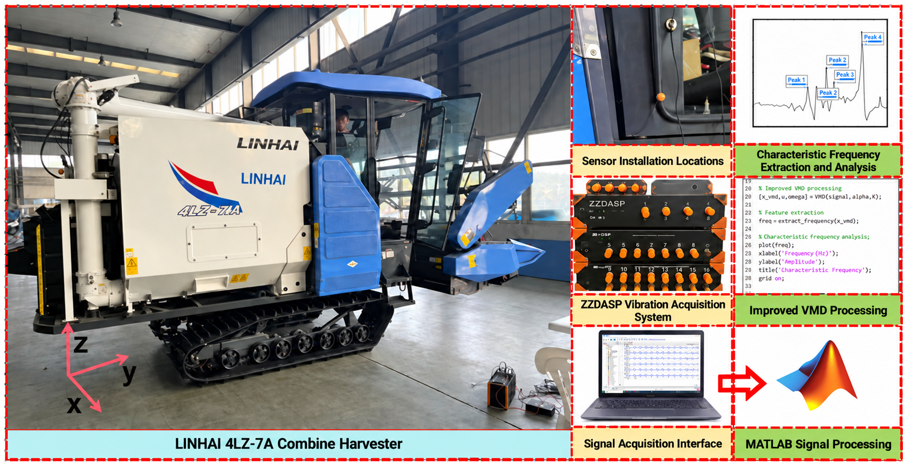
A Linhai 4LZ-7A tracked combine harvester was selected as the test machine. It was equipped with a V36-150C42 inline four-cylinder, water-cooled, four-stroke, direct-injection, turbocharged and intercooled engine with a rated speed of 2400 r/min. Before modification, the cab was connected to the frame through four support points without vibration isolation elements. Vibration signals were acquired using a ZZDASP system and one YX-1182 triaxial piezoelectric accelerometer; the sensor parameters are listed in

Table 1. Basic parameters of the YX-1182 piezoelectric sensor.

Sensor Model	Frequency Range	Operating Voltage	Sensitivity
YX-1182	0.5–5000 Hz	18–28 V	10.051 mV/(m/s2)

. The accelerometer was magnetically attached at the measurement locations shown in Figure 1, and the X, Y and Z channels were acquired synchronously. The sampling frequency was 12,800 Hz, with 1,000,000 samples per channel per record, corresponding to 78.125 s. The X, Y and Z axes correspond to the transverse, forward and vertical directions of the harvester, respectively. Signal analysis was performed in MATLAB 2020.

2.2. Vibration Test Conditions and Excitation Frequencies of the Main Components

The tests addressed excessive cab vibration after machine manufacture during stationary no-load operation, with no crop feeding. Under Condition A, only the engine was running. Under Condition B, the engine, threshing drum, vibrating screen, cutter, conveying device, cleaning fan and straw chopper were running. The tracks remained stationary in both conditions. The measured engine speed fluctuated within 2390–2500 r/min. Three vibration records were acquired under each condition, and selected records were used for the subsequent signal analysis; the reported signal analysis results are not pooled statistics from all three records.

Table 2. On-site measured component speed ranges and corresponding rotational frequencies during the tests.

No.	Component	Speed Range Under Normal Operation (r/min)	Excitation Frequency Range (Hz)
1	Engine	2390–2500	39.8–41.67
2	Threshing drum	690–730	11.50–12.17
3	Vibrating screen	416–476	6.93–7.93
4	Cutter	555–635	9.25–10.58

gives the on-site measured speed ranges and corresponding rotational frequencies of the listed components. Speed records corresponding to the selected vibration records were retained. The tests do not cover ground excitation during travel, crop feeding or changes in grain-tank load.

2.3. Vibration Signal Processing Algorithm Based on Hybrid Grey Wolf–Whale Optimized VMD

2.3.1. Variational Mode Decomposition Theory

Variational mode decomposition (VMD) is an advanced signal processing method whose core idea is to adaptively decompose the original signal into a series of intrinsic mode functions (IMFs) with specific center frequencies and bandwidths by constructing a variational problem [30]. The aim is to decompose the signal f(t) into K modes u_k(t), each centered on a frequency ω_k, while minimizing the sum of the bandwidths of all modes. Through optimization within the variational framework, the signal is segmented in the frequency domain [34,35]. The mathematical model is as follows:

$$\underset{\left\{u_k\right\},\left\{{\omega }_k\right\}}{min}{\displaystyle \sum _{k=1}^K{‖\frac{\partial }{{\partial }_t}\left[\left(\delta \left(t\right)+\frac{j}{\pi t}\right)\times u_k\left(t\right)\right]e^{-j{\omega }_{k}t}‖}_2^2}$$

(1)

$$s.t.{\displaystyle \sum _{k=1}^K{u}_k\left(t\right)=f\left(t\right)}$$

(2)

Here, u_k(t) is the kth mode, ω_k its center frequency, ∂_t the time derivative, and δ(t) the Dirac delta function. The Hilbert transform provides the analytic representation of each mode.

The MATLAB lowpass function was applied with a cutoff frequency of 100 Hz and steepness set to 0.95. The reference spectral band used for evaluation matched this cutoff and covered the prescribed target frequencies. This setting restricted the frequency range supplied to VMD; it was not selected through a cutoff-sensitivity study. Components near the cutoff were not assumed to be unaffected by attenuation.

2.3.2. Grey Wolf Optimizer and Whale Optimization Algorithm

In the grey wolf optimizer (GWO) [32], α, β and δ denote the best, second-best and third-best candidate solutions, respectively; the remaining candidates are denoted by ω. These hierarchy labels are distinct from the VMD penalty factor α. The position update is expressed as follows:

$$\overrightarrow{D}=\left|\overrightarrow{C}\cdot {\overrightarrow{X}}_p-\overrightarrow{X}\right|$$

(3)

$$\overrightarrow{X}\left(t+1\right)=\overrightarrow{X_p}-\overrightarrow{A}\cdot \overrightarrow{D}$$

(4)

where $\overrightarrow{A}=2a\overrightarrow{r_1}-a$, $\overrightarrow{C}=2\overrightarrow{r_2}$, and $a=2-{\displaystyle \frac{2t}{t_{max}}}$.

During the hunting process:

$$\overrightarrow{D_a}=\left|\overrightarrow{C}\cdot {\overrightarrow{X}}_a-\overrightarrow{X}\right|$$

(5)

$$\overrightarrow{X_1}={\overrightarrow{X}}_a-\overrightarrow{A}\cdot \overrightarrow{D_a}$$

(6)

By analogy, $\overrightarrow{X_2}$ and $\overrightarrow{X_3}$, the following is obtained:

$$\overrightarrow{X}\left(t+1\right)={\displaystyle \frac{\overrightarrow{X_1}+\overrightarrow{X_2}+\overrightarrow{X_3}}{3}}$$

(7)

Here, the arrow denotes a vector. X is a candidate position, X_p is the prey position, D is the distance vector, and A and C are coefficient vectors. The vectors r₁ and r₂ are uniformly distributed random vectors. The scalar a is the convergence factor, t is the iteration index, and t_max is the maximum iteration number. The α, β and δ subscripts identify the three leading wolves; analogous updates give X₂ and X₃.

When the whale optimization algorithm (WOA) encircles the prey [33]:

$$\overrightarrow{D}=\left|\overrightarrow{C}\cdot \overrightarrow{X^{\ast }}-\overrightarrow{X}\right|$$

(8)

$$\overrightarrow{X}\left(t+1\right)=\overrightarrow{X^{\ast }}-\overrightarrow{A}\cdot \overrightarrow{D}$$

(9)

where $\overrightarrow{A}=2a\overrightarrow{r_1}-a$, $\overrightarrow{C}=2\overrightarrow{r_2}$, and $a=2-{\displaystyle \frac{2t}{t_{max}}}$.

A spiral update is then performed to simulate the bubble-net attacking strategy:

$$\overrightarrow{X}\left(t+1\right)=\overrightarrow{D^{\prime }}\cdot e^{bl}\cdot cos\left(2\pi l\right)+\overrightarrow{X^{\ast }}$$

(10)

$$\overrightarrow{D^{\prime }}=\left|\overrightarrow{X^{\ast }}-\overrightarrow{X}\right|$$

(11)

Here, b is the spiral-shape constant and l is a random number in [−1, 1].

Finally, a random search is performed:

$$\overrightarrow{X}\left(t+1\right)={\overrightarrow{X}}_{\mathrm{rand}}-\overrightarrow{A}\cdot \overrightarrow{D}$$

(12)

Here, $\overrightarrow{X}$ is the current best whale position, $\overrightarrow{D}$ is its distance from the current candidate, and ${\overrightarrow{X}}_{\mathrm{rand}}$ is a randomly selected whale position. $\overrightarrow{A}$ and $\overrightarrow{C}$ are coefficient vectors; r₁ and r₂ are uniformly distributed random vectors. The scalar a is the convergence factor. The factors $e^{bl}$ and cos(2πl) define the spiral update. Arrows denote vectors.

2.3.3. Theory of the Hybrid Grey Wolf–Whale Optimized VMD Algorithm

The hybrid optimizer combined the leader-based GWO update with the spiral update of WOA. At iteration t, the probability of selecting the GWO update was:

$$p\left(t\right) = 0.45 + 0.15 cos\left({\displaystyle \frac{\pi t}{t_{max}}}\right)$$

(13)

For each candidate and each parameter coordinate, an independent uniform random draw r in [0, 1) selected GWO when r < p(t); otherwise, the WOA spiral update was applied. Thus, p(t) was a probability rather than a deterministic threshold on the iteration index. The convergence factor was:

$$a\left(t\right) = 2 -{\displaystyle \frac{2t}{t_{max}}}$$

(14)

The parameter vector comprised the integer mode number K and the penalty factor α:

$$\theta = (K, \alpha ), K \in \{3, 4, 5, 6, 7, 8\}, \alpha \in [800, 5000]$$

(15)

The population contained eight candidates. Five tent-map transformations of uniformly distributed random values preceded scaling to the parameter bounds. Candidate values were clipped to these bounds, and K was rounded to the nearest integer for fitness evaluation. The optimizer evaluated the initial population and then performed 12 update iterations, retaining the best fitness found. One seeded run was performed per analyzed channel and condition; the curves represent the history within that run, not variability across independent runs. Fitness evaluation used a resampled input at 1000 Hz to reduce computational cost.

For each candidate pair, VMD decomposed the input x(n) into K modes u_k(n). Selected modes were summed and projected onto the prescribed target-frequency bands to obtain y(n) for spectral evaluation. The composite fitness was minimized:

$$F(K, \alpha ) = -R_T+ 0.65R_I+ 0.20E_r+ 0.015K$$

(16)

Here, R_T and R_I are the target-frequency and interference-frequency energy ratios defined below. The normalized reconstruction error E_r used all K modes before mode selection and frequency projection:

$$E_r={\displaystyle \frac{RMS\left[x\right(n) -{\sum }_{k=1}^K{u}_k\left(n\right)]}{max\left(RMS\right[x\left(n\right)], \epsilon )}}$$

(17)

RMS is the square root of the mean squared sample value, and ε is MATLAB machine epsilon. The negative target-energy term rewards relative concentration near the target frequencies. Positive interference and reconstruction-error terms penalize selected interference components and incomplete reconstruction by the full mode set. The term 0.015 K penalizes mode count; it does not directly measure inter-mode correlation or spectral overlap. The weights 1, 0.65, 0.20 and 0.015 were fixed design coefficients, not additional optimization variables. They express the intended trade-off among these criteria. The contribution of each term also depends on its observed scale. A failed fitness evaluation received a penalty of 10⁶.

For a signal being evaluated, its mean was removed, and a periodic Hann window was applied. The single-sided amplitude spectrum A(f_m) was obtained by FFT, normalized by the sum of the window coefficients, with non-DC and non-Nyquist amplitudes doubled. Spectral energy here denotes the sum of squared spectral amplitudes, rather than physical mechanical energy or an explicitly estimated power spectral density. The reference energy was:

$$E_0={\sum }_{0\le f_m\le 100 \mathrm{H}\mathrm{z}}{A}^2\left(f_m\right)$$

(18)

Let f_T,j and f_I,j denote the prescribed target and interference frequencies, respectively, with N_T and N_I entries. The energy in each frequency neighborhood was accumulated using the common half-width Δf = 1.2 Hz:

$$E_T={\sum }_{j=1}^{N_T}{\sum }_{|f_m-f_{T,j}|\le \Delta f}{A}^2\left(f_m\right)$$

(19)

$$E_I={\sum }_{j=1}^{N_I}{\sum }_{|f_m-f_{I,j}|\le \Delta f}{A}^2\left(f_m\right)$$

(20)

The corresponding normalized energy ratios were:

$$R_T={\displaystyle \frac{E_T}{max(E_0, \epsilon )}}$$

(21)

$$R_I={\displaystyle \frac{E_I}{max(E_0, \epsilon )}}$$

(22)

A larger R_T indicates greater relative energy in the selected target neighborhoods, whereas a smaller R_I indicates less relative energy in the selected interference neighborhoods. Spectral purity η compares these two components directly:

$$\eta ={\displaystyle \frac{E_T}{max(E_T+E_I, \epsilon )}}$$

(23)

Spectral purity lies between 0 and 1. A value near 1 indicates that target energy dominates the sum of the selected target and interference energies. Energy outside both sets of neighborhoods is absent from its denominator, so high purity does not establish low noise throughout the spectrum. If both energies are zero, the implementation returns zero; this degenerate case has no usual purity interpretation. These metrics describe relative spectral allocation, not independent source-identification accuracy.

The frequency sets were specified separately for each condition and direction, rather than derived from retained or excluded VMD center frequencies. Under Condition A, the target frequencies were {40.96, 81.92} Hz for all directions. The interference frequencies were {7.68, 10.24, 20.48, 28.16, 29.44, 38.40, 58.88, 72.96} Hz.

Under Condition B, the target sets for X, Y and Z were {7.68, 10.24, 81.92}, {7.68, 10.24, 40.96, 58.88, 81.92} and {7.68, 40.96, 58.88, 72.96, 81.92} Hz, respectively. The corresponding interference sets were {28.16, 29.44, 38.40, 40.96, 58.88, 72.96}, {28.16, 29.44, 38.40, 72.96} and {10.24, 28.16, 29.44, 38.40} Hz. These labels define the extraction task for a given channel; an excluded target in one channel is not thereby established as physical noise.

The reference band of 0–100 Hz matched the low–pass cutoff and displayed the spectral range and contained the prescribed target frequencies. All methods used the same band within a channel and condition. This was an application-specific analysis range, not an experimentally optimized cutoff. The ±1.2 Hz evaluation tolerance allowed energy accumulation around a prescribed frequency rather than at a single spectral bin. Its purpose was to accommodate small peak offsets while limiting inclusion of neighboring components; its optimality was not established by measured frequency-drift statistics or a tolerance-sensitivity study. The FFT length gave a frequency-grid spacing no larger than approximately 0.125 Hz. This spacing is distinct from the evaluation tolerance and does not, by itself, specify the resolving ability of the finite, windowed record.

Energy ratios were normalized by the reference energy of each evaluated signal, whereas purity was normalized by the sum of its selected target and interference energies. Except when the ε safeguard dominates, uniform amplitude scaling cancels from these ratios. The normalization supports comparison of relative spectral composition across signals with different amplitudes but cannot demonstrate recovery of absolute target amplitudes. Target-frequency amplitudes and RMS therefore provide complementary information. Because E_T and E_I sum neighborhoods separately, overlapping neighborhoods are counted repeatedly. R_T and R_I are not guaranteed to remain below 1. Overlap between target and interference neighborhoods can also contribute to both terms; η remains bounded but depends on the prescribed sets.

The target-frequency projection used a separate half-width for each target:

$$b_j= max(1.2 Hz, 0.08f_{T,j})$$

(24)

It retained the union of these bands, removed frequencies above 100 Hz, and preserved the conjugate-frequency counterparts for a real-valued reconstruction. Unlike the fixed evaluation tolerance, this processing bandwidth increased with target frequency above the minimum half-width. The factor 0.08 was a fixed setting, not a validated optimum. With S denoting the selected mode indices and P_B the FFT masking and inverse transform and truncation to the input length, the signal used for spectral scoring was:

$$y\left(n\right) =P_B\left[{\sum }_{k\in S}{u}_k\left(n\right)\right]$$

(25)

Mode selection combined target-energy concentration, dominant-frequency proximity, absolute correlation with the input, kurtosis and an interference-energy penalty. Thus, the spectral terms in the fitness measure the combined decomposition, selection and projection procedure. The full-mode error in Equation (17) does not measure the final projected output error. Reported improvements in spectral metrics cannot be assigned to parameter optimization alone.

The best evaluated candidate minimized the fitness over the candidates visited during the run:

$$(K^{*},{\alpha }^{*}) ={arg min}_{(K, \alpha ) \in C}F(K, \alpha )$$

(26)

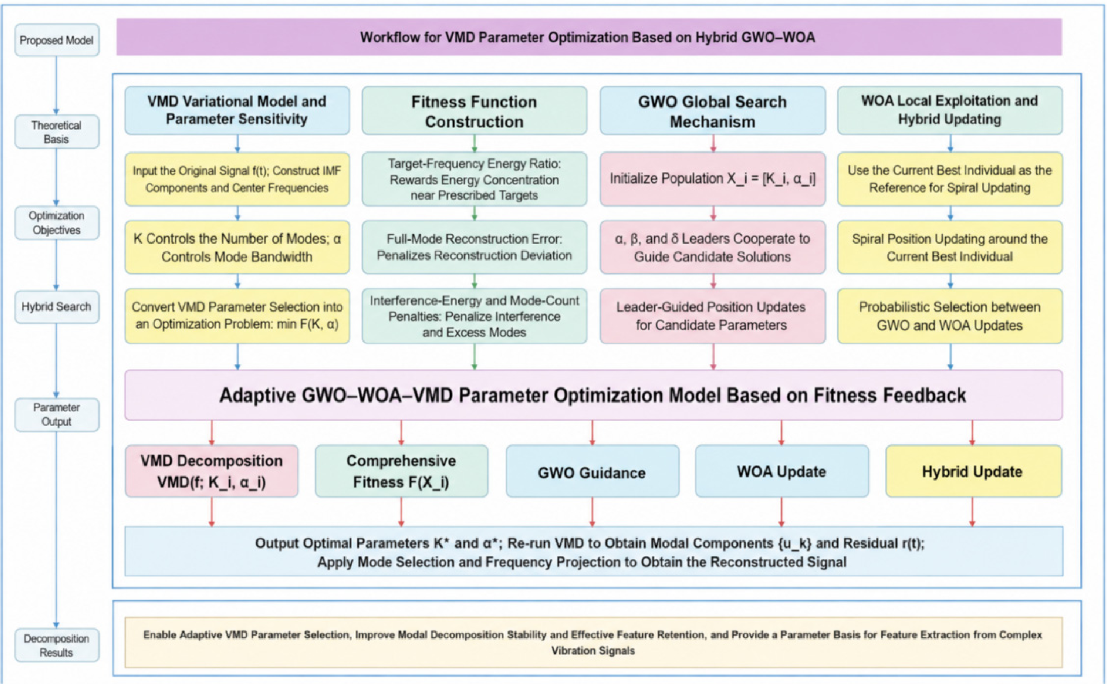
Here, C is the set of evaluated candidate pairs. The returned penalty factor was rounded to the nearest integer and bounded before the final VMD run. Candidate decompositions used peak initialization, a maximum of 300 iterations, an absolute tolerance of 10⁻⁶ and a relative tolerance of 10⁻⁴. Final decomposition used the original sampling rate, target-informed spectral-peak initialization, a maximum of 800 iterations, an absolute tolerance of 10⁻⁷, and a relative tolerance of 10⁻⁴. Consequently, the logged best fitness belongs to the candidate evaluation, not a fresh evaluation of the final decomposition. Figure 2 summarizes this procedure.

In the comparison implementation, conventional VMD used a penalty factor of 2000 and K = max(4, min(6, N_c + 2)), where N_c is the number of configured comparison target frequencies. It used peak initialization and a maximum of 500 iterations. Mode selection used the composite spectral-feature score and a cap on the number of retained modes. For Condition A, the comparison targets were {40.96, 55.04, 81.92} Hz for X, {12.80, 40.96, 55.04, 58.88, 83.20} Hz for Y and {40.96, 49.92, 57.60} Hz for Z. Additional Gaussian-shaped spectral gains were applied to the conventional VMD reconstruction: 0.58 at 58.88 Hz for X, 2.45 at 12.80 Hz for Y and 0.25 at 81.92 Hz for Z, with width parameters of 3.0, 2.4 and 3.5 Hz, respectively. These processing differences are part of the comparison and prevent attributing its full effect to VMD parameter selection alone. Changes in reconstructed RMS describe signal processing, whereas mechanical vibration reduction was evaluated separately using measured acceleration records in Section 4.4.

3. Results

3.1. VMD-Based Vibration Signal Analysis

3.1.1. Time–Frequency-Domain Analysis of the X-Direction Vibration Signal of the Cab Under Condition A

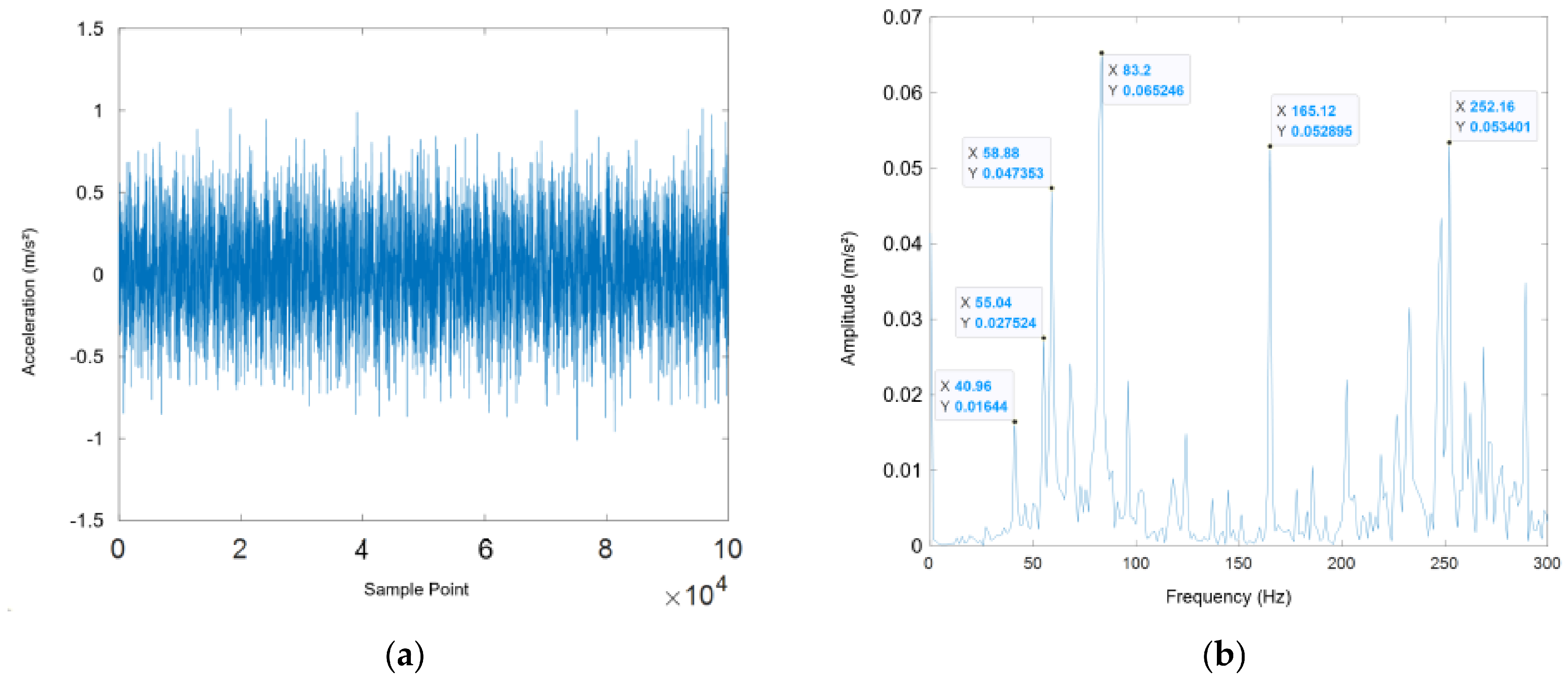
The original X−direction cab vibration signal under Condition A is shown in Figure 3. For both Conditions A and B, the middle 100,000 samples of the selected record were used for analysis, corresponding to 7.8125 s at 12,800 Hz. This selection avoided possible operating adjustments or transient fluctuations at the beginning and end of the record. The same start and end sample indices were used for the X, Y and Z channels of a given record.

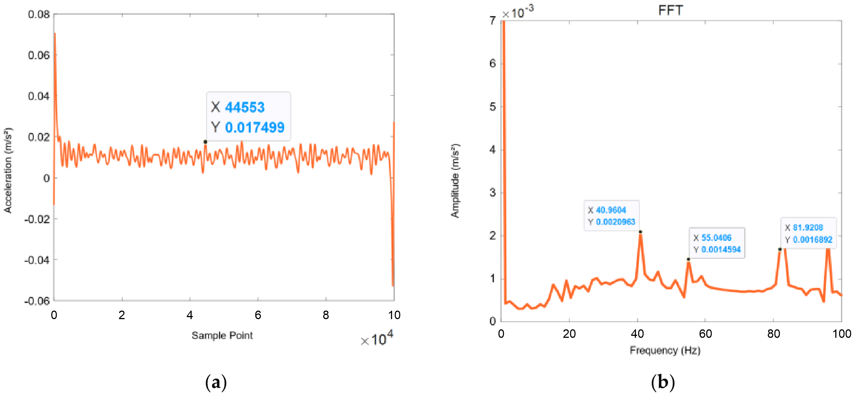
As shown in Figure 3, the original X−direction acceleration has peaks exceeding 1 m/s² and an RMS value of 0.2848 m/s². The spectral components at 40.96 and 81.92 Hz fall within the measured engine rotational and second-order frequency ranges, respectively. With only the engine running under Condition A, these components are consistent with engine-related excitation. The additional higher-frequency components are retained as observations without assigning specific excitation mechanisms or transfer paths. Figure 4 presents the signal after low–pass filtering.

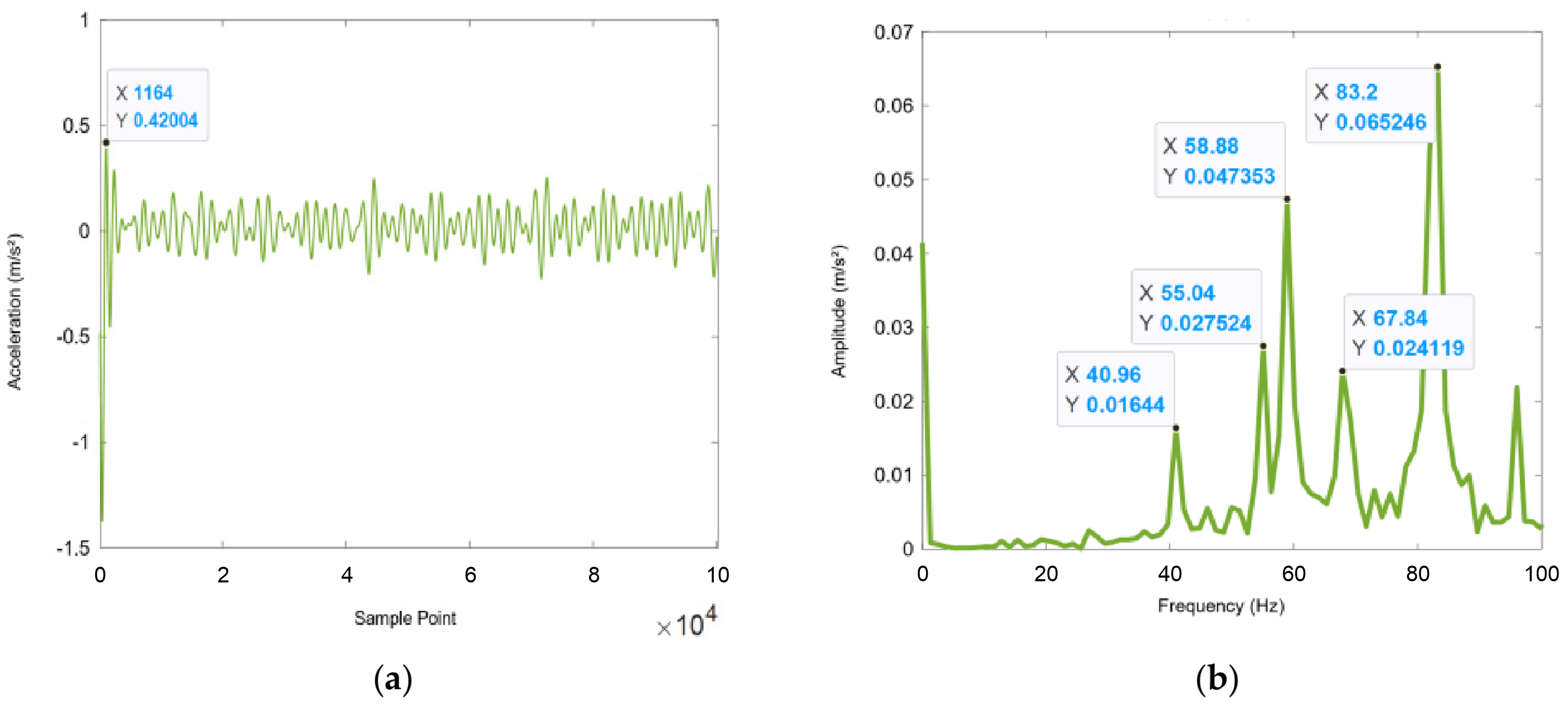
After low-pass filtering, the peak acceleration is 0.42 m/s² and the RMS value is 0.0875 m/s² (Figure 4). The reduction from the original RMS of 0.2848 m/s² reflects attenuation of signal components rather than a reduction in machine vibration. The principal components below 100 Hz remain visible. The filtered signal was decomposed into five modes using conventional VMD. IMF2 and IMF3 were retained for reconstruction according to the screening procedure in Section 2.3; IMF1, IMF4 and IMF5 were not included. Figure 5 shows the reconstructed signal [30].

After conventional VMD reconstruction, the X–direction RMS is 0.012 m/s² and the peak acceleration is approximately 0.0175 m/s² (Figure 5). The spectrum contains components at 40.96 Hz (0.0021 m/s²) and 81.92 Hz (0.0018 m/s²). The 67.84 Hz component is not retained in the reconstruction, while additional spectral components remain.

3.1.2. Time–Frequency–Domain Analysis of the Y–Direction Vibration Signal of the Cab Under Condition A

The time-domain waveform and frequency spectrum of the original Y-direction vibration signal of the cab under Condition A are shown in Figure 6.

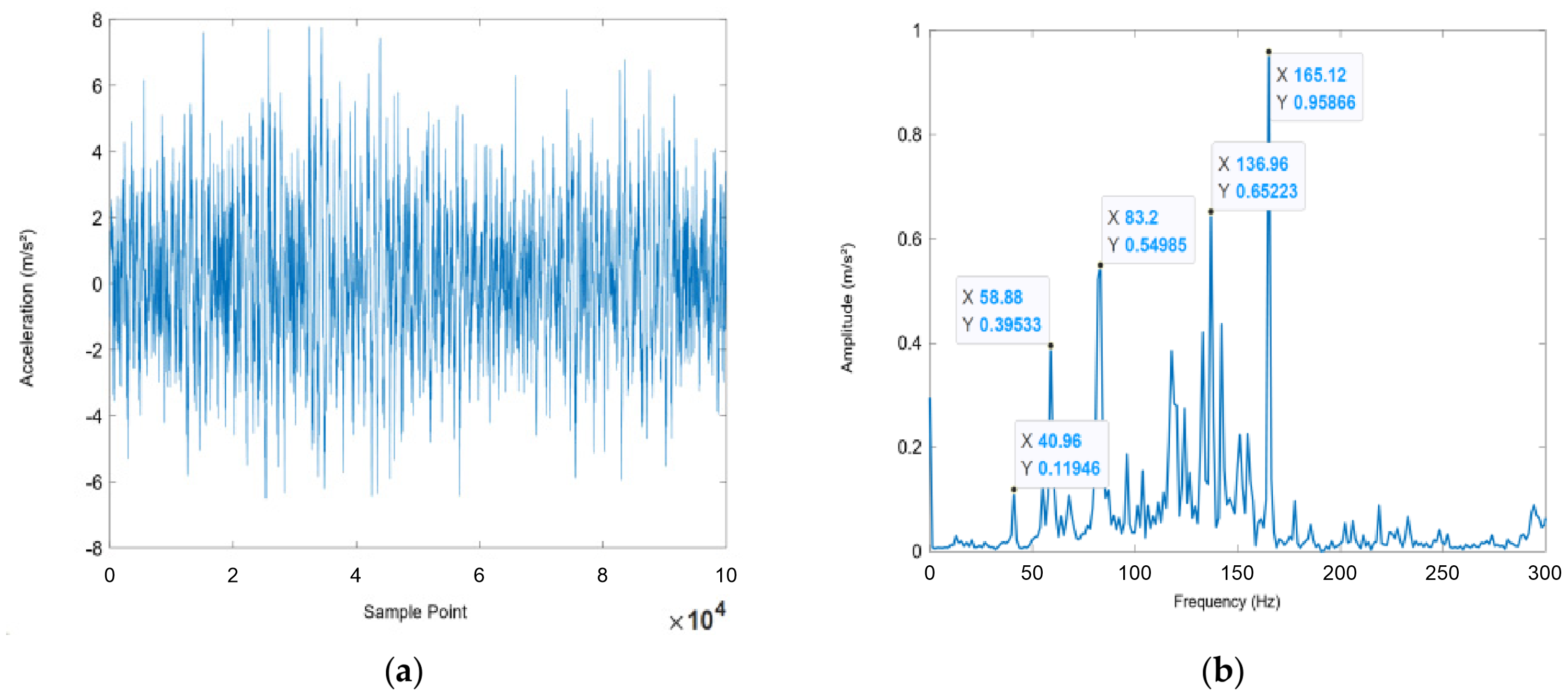
The original Y–direction acceleration has peaks exceeding 6 m/s² and an RMS value of 1.8626 m/s² (Figure 6). Components occur at 40.96, 83.2, 165.12, 136.96 and 58.88 Hz. The component near 83.2 Hz is consistent with engine second-order excitation. The spectrum also contains a component at 58.88 Hz, which may be associated with the dynamic response of the cab system. These observations are not used to confirm acoustic–structural coupling resonance. Figure 7 shows the low–pass–filtered signal.

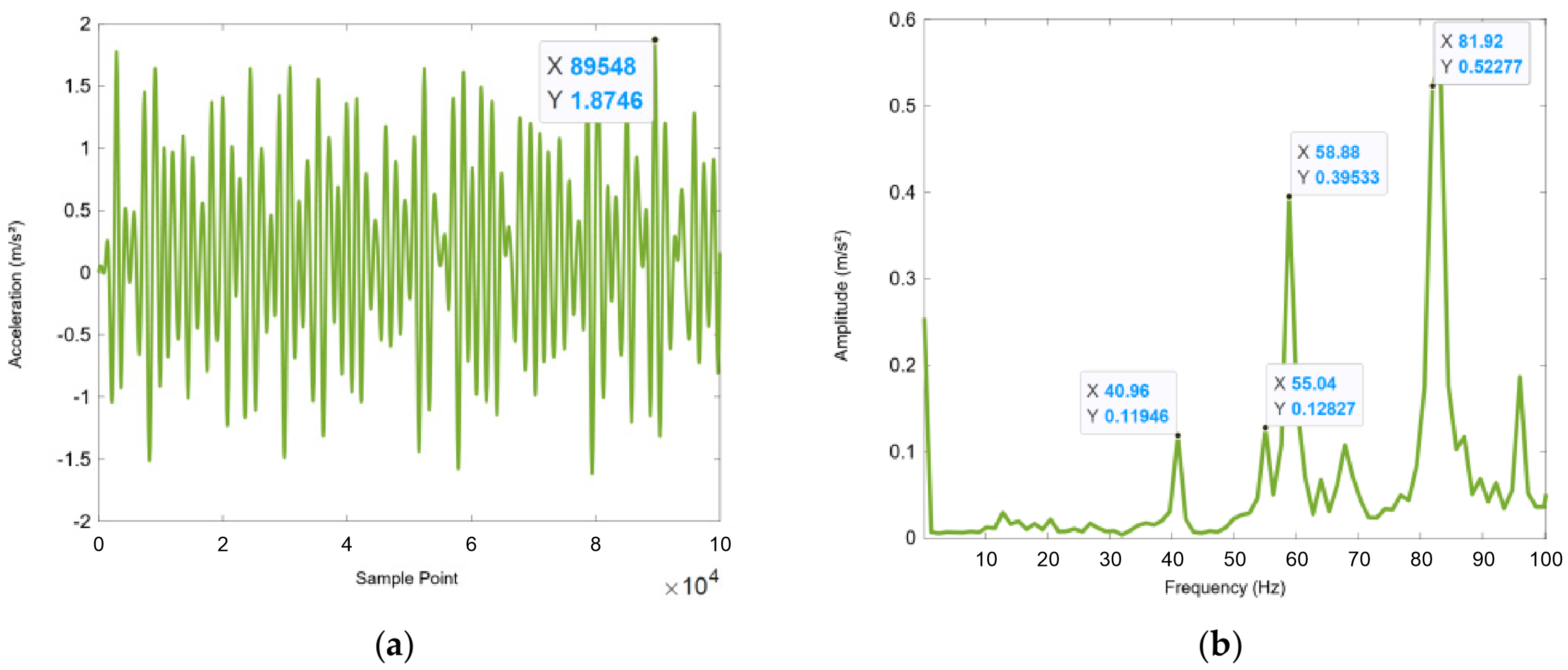
After low-pass filtering, the Y–direction peak acceleration is 1.8746 m/s² and the RMS value is 0.7208 m/s² (Figure 7). Components at 81.92, 40.96 and 58.88 Hz are visible. The filtered signal was decomposed into five modes. IMF2 and IMF3 were retained for reconstruction, whereas IMF1, IMF4 and IMF5 were excluded. The resulting waveform and spectrum are shown in Figure 8.

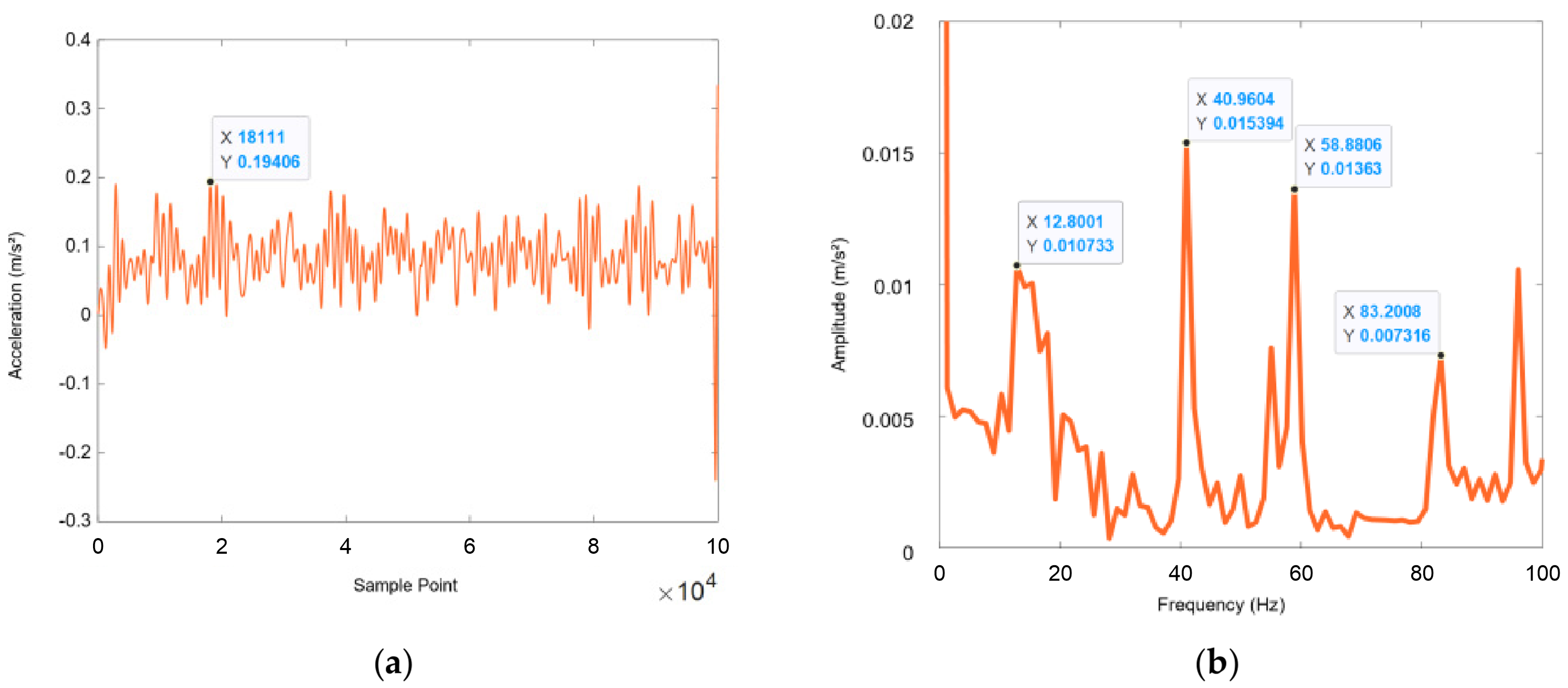
The reconstructed Y–direction signal has an RMS value of 0.0924 m/s² and a periodic waveform (Figure 8). Components at 40.96 and approximately 83.2 Hz remain visible, consistent with the engine rotational frequency and second-order excitation. Additional components remain in the spectrum. The RMS change reflects signal reconstruction and does not measure mechanical vibration reduction.

3.1.3. Time–Frequency–Domain Analysis of the Z–Direction Vibration Signal of the Cab Under Condition A

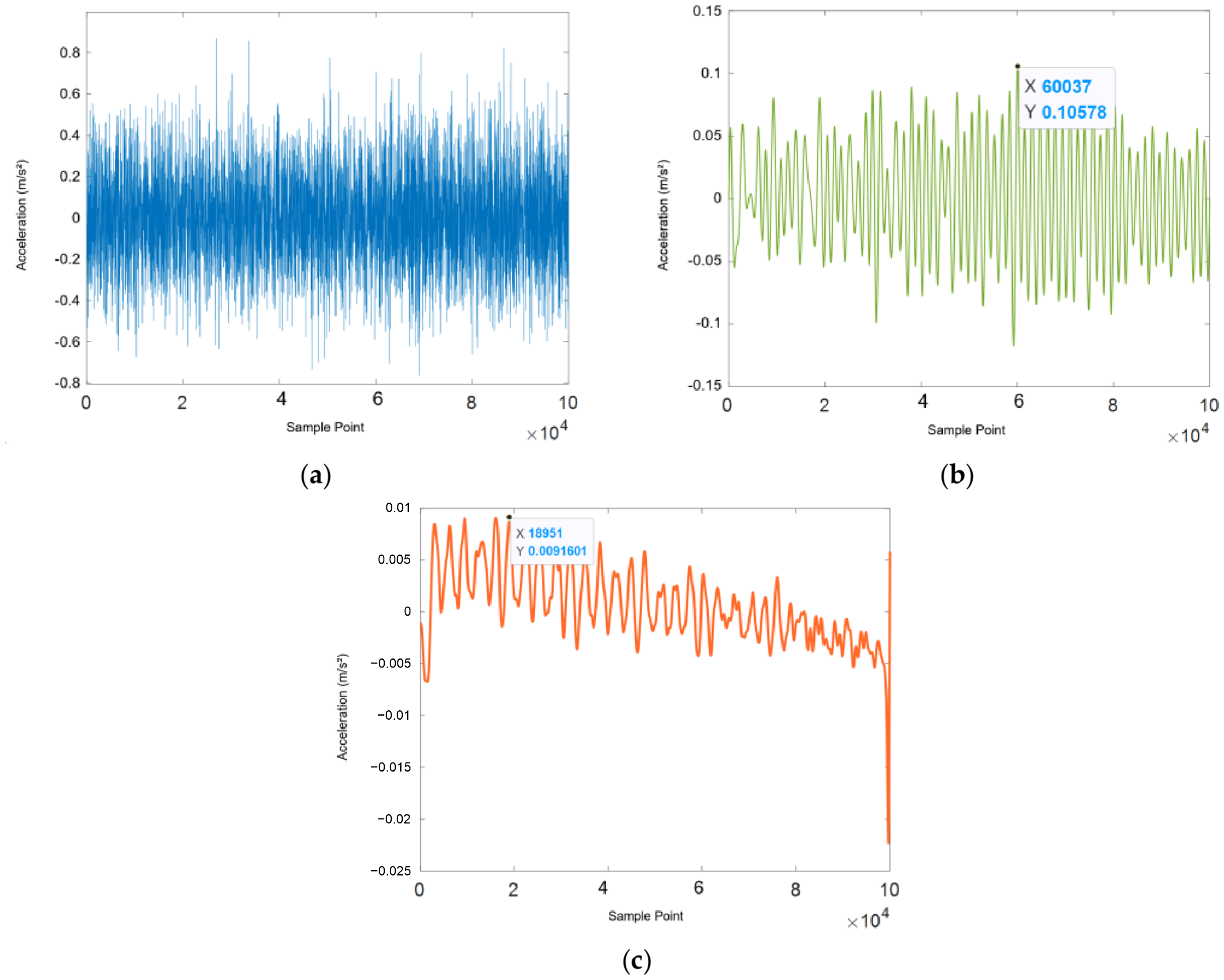
The time-domain waveform of the Z–direction vibration signal of the cab under Condition A is shown in Figure 9. After low-pass filtering and after the combined low–pass filtering and VMD processing, the reconstructed time-domain waveforms show obvious periodic positive–negative alternation, and the peak accelerations decrease. After VMD decomposition, the peak acceleration is 0.009 m/s², and the RMS values of the three signals are 0.2000, 0.0445 and 0.0037, respectively.

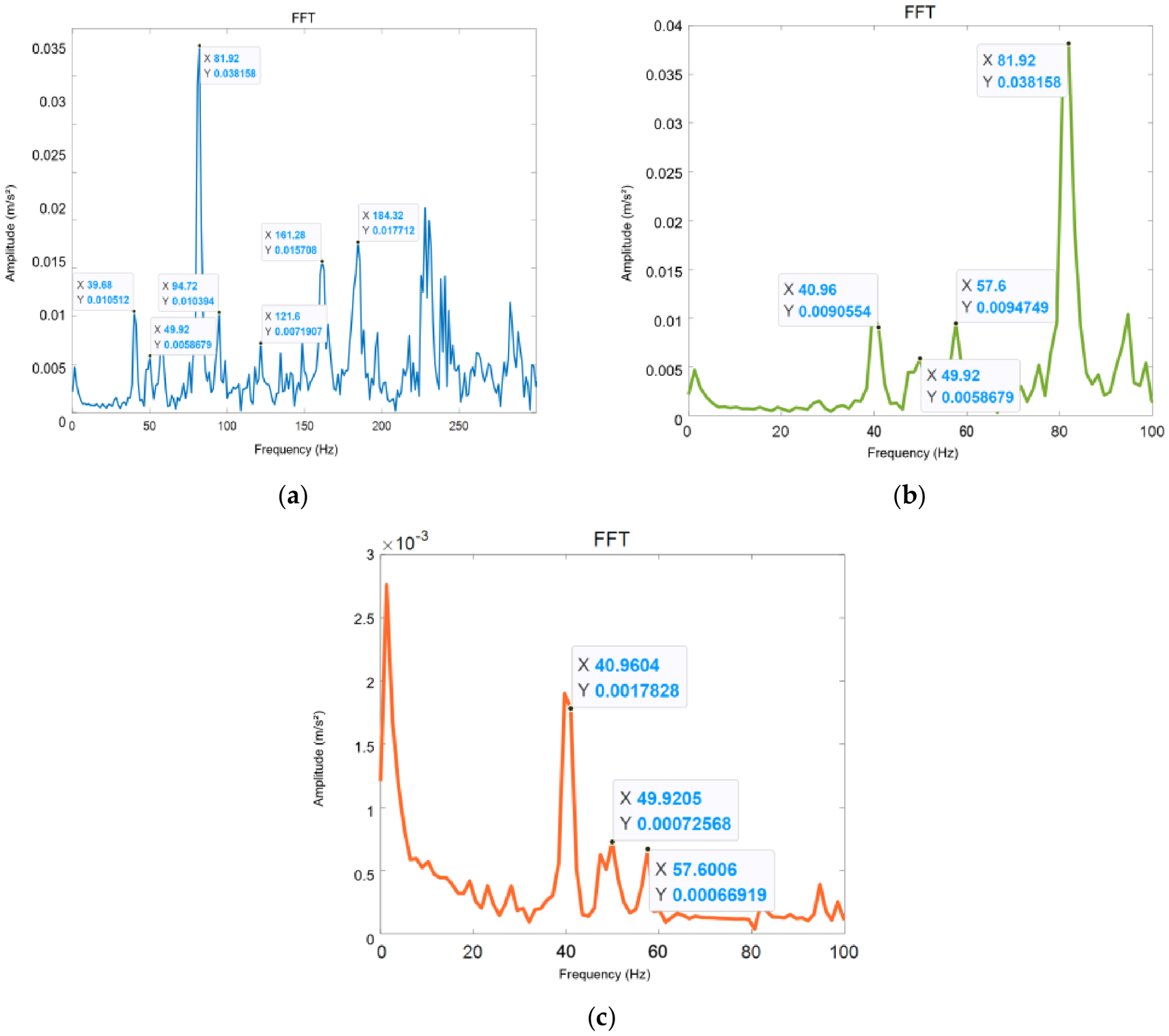
After low-pass filtering, the Z–direction spectrum contains prominent components at 81.92, 57.6 and 40.96 Hz (Figure 10). The components at 40.96 and 81.92 Hz are consistent with engine rotation and second-order excitation. The 57.6 Hz component is reported as an additional observed component without an engine order or resonance assignment. Following conventional VMD reconstruction, the 81.92 Hz component is attenuated and the 40.96 Hz component becomes more prominent; components at 49.9 and 57.6 Hz remain.

The conventional VMD results illustrate the sensitivity of feature extraction to manually specified parameters and mode screening for these signals. The frequencies of interest are concentrated below 100 Hz, where several components are closely spaced. The comparison concerns the reported parameter settings and does not establish a general limitation of conventional VMD. Under Condition B, the engine and working components operate simultaneously, whereas the tracks are stationary. The frame and cab participate in vibration transmission and response; the tracks are not treated as an active excitation source in these tests.

3.2. HGWO-VMD-Based Vibration Signal Analysis

3.2.1. Vibration Signal Analysis of the Cab in the X Direction Under Condition A

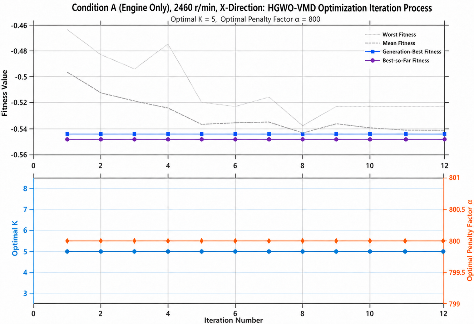
For the X–direction signal under Condition A, the single HGWO–VMD optimization run yielded K = 5 and α = 800. Figure 11 shows the parameter evolution during that run.

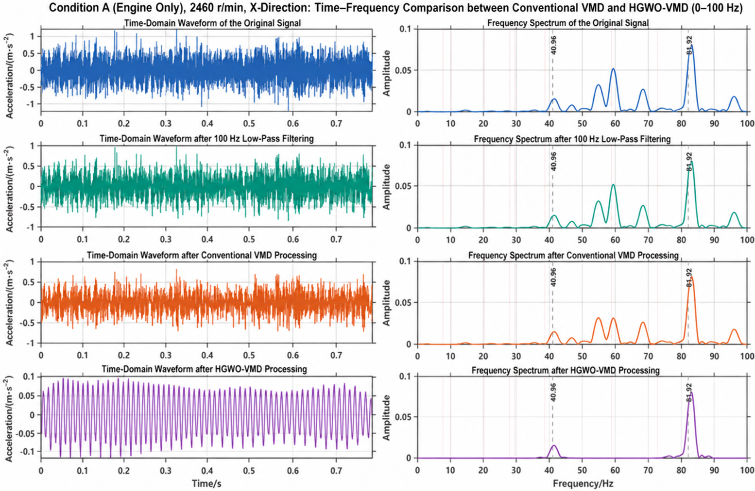
Figure 12 compares the X–direction signals processed using HGWO–VMD and conventional VMD under Condition A. Components near 40.96 and 81.92 Hz are prominent in the HGWO–VMD reconstruction and are consistent with engine rotation and second–order excitation. The comparison shows differences in the retained spectral content for these settings; it does not independently identify combustion forces, inertial forces or transfer paths.

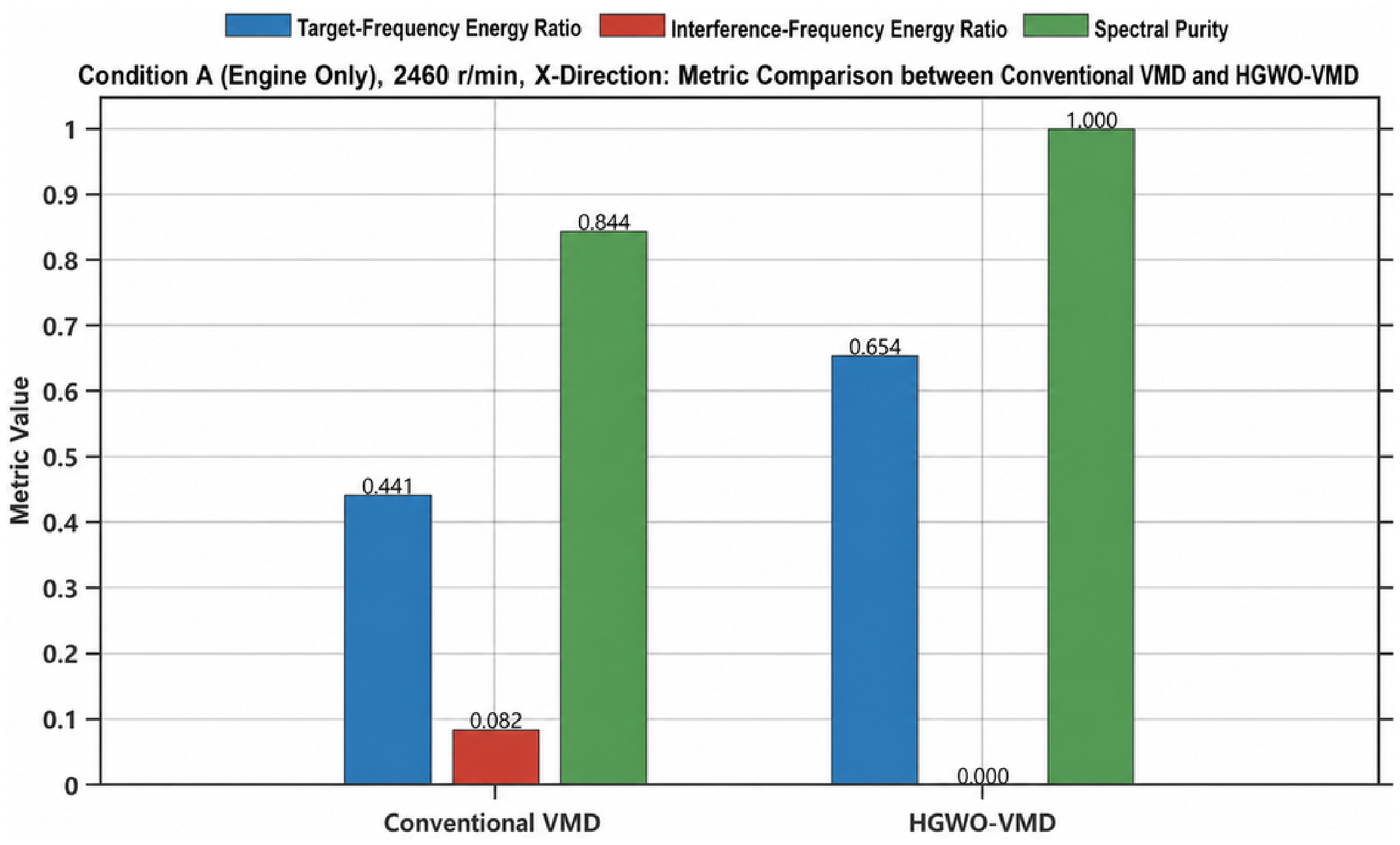
Figure 13 compares the metrics defined in Section 2.3 for the X–direction signal under Condition A. Conventional VMD gives R_T = 0.441, R_I = 0.082 and η = 0.844. HGWO-VMD gives R_T = 0.654, with R_I close to zero and η close to 1. These values indicate a higher relative concentration of energy in the selected target bands; they do not demonstrate complete removal of noise or all non-target components.

3.2.2. Vibration Signal Analysis of the Cab in the Y Direction Under Condition A

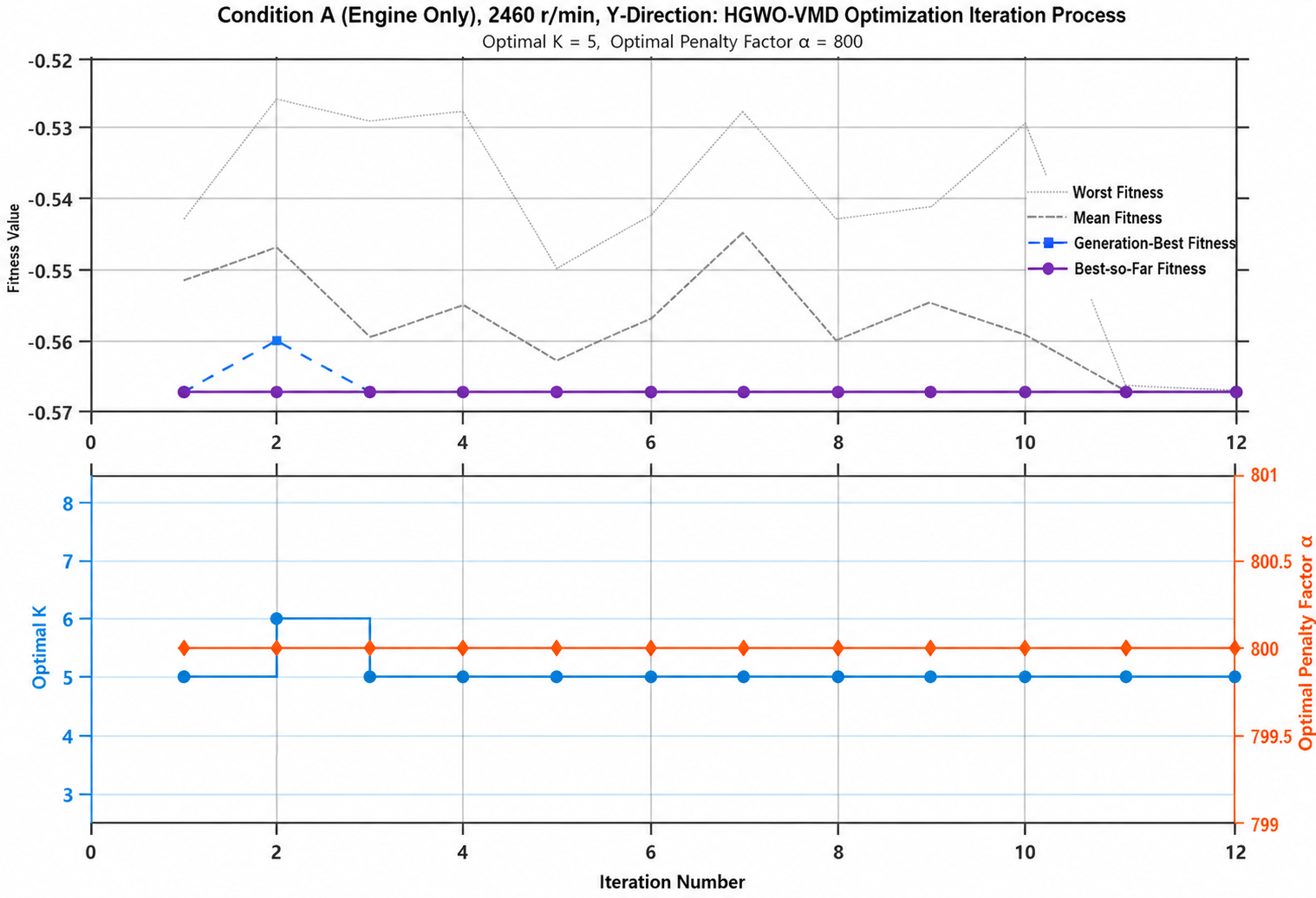
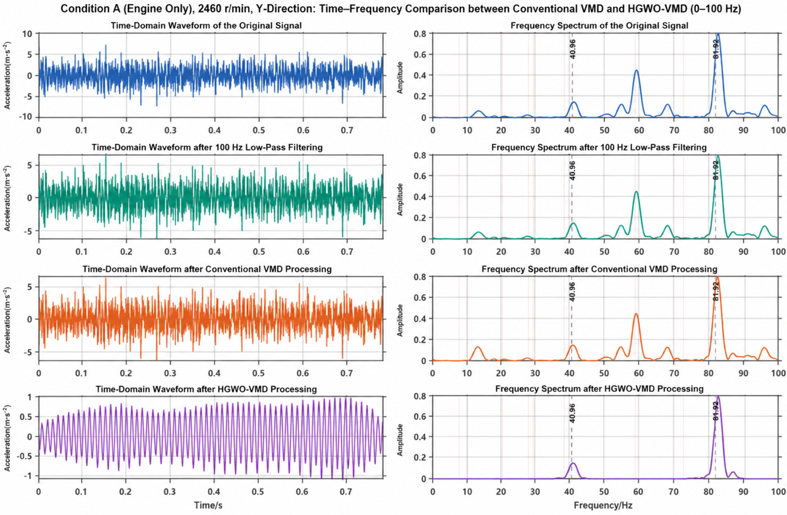
The Y–direction vibration signal of the cab was processed; the iteration results of the adaptive mode number and penalty factor optimization based on HGWO–VMD are shown in Figure 14. The optimization yielded a mode number of K = 5 and a penalty factor of α = 800. VMD with the optimized parameters was used to decompose the vibration signal, and the results were compared with the original signal, the low-pass filtered signal and the conventional VMD-processed signal in the time and frequency domains, as shown in Figure 15.

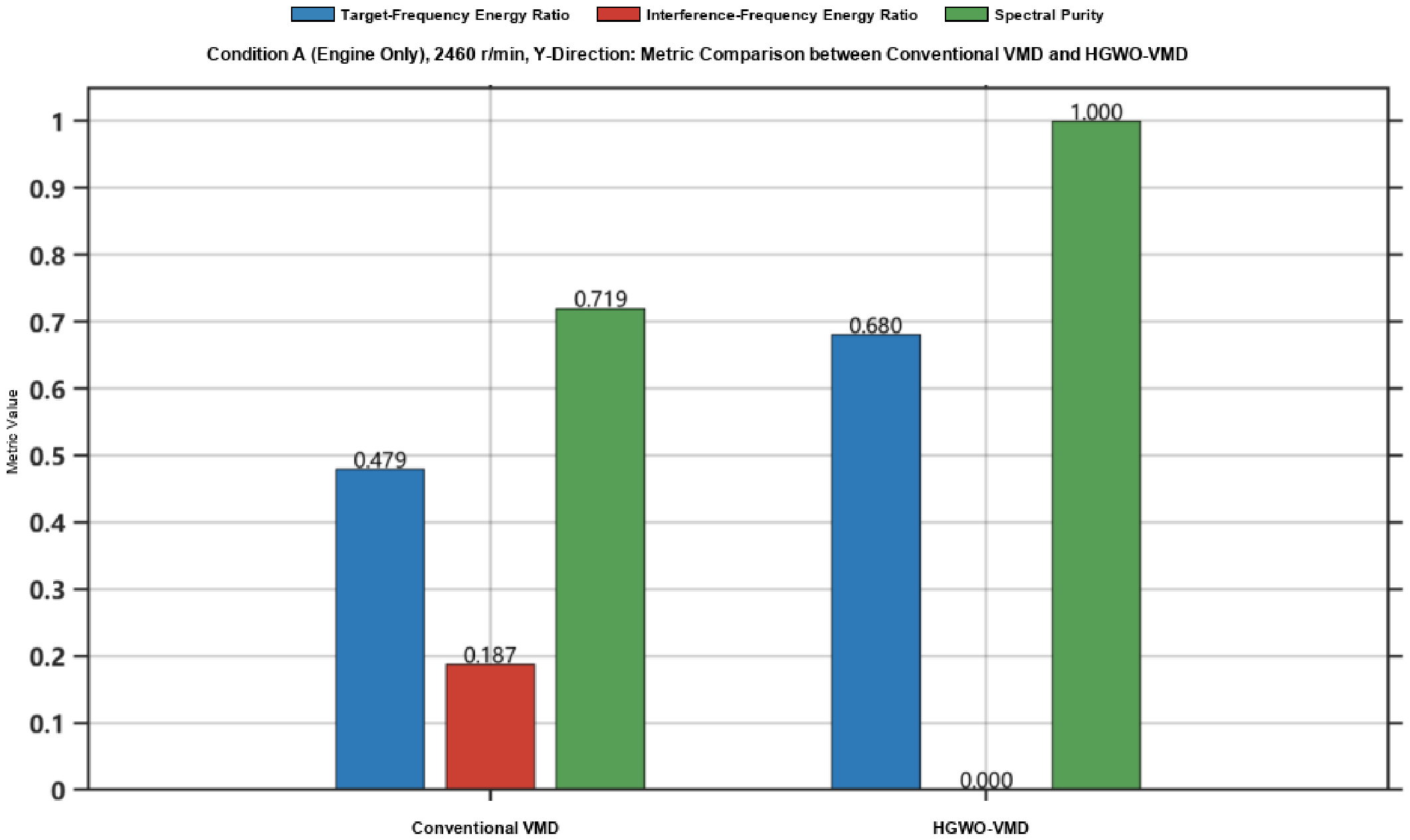
Figure 15 shows that the HGWO–VMD reconstruction has a more regular waveform and prominent components near 40.96 Hz and the engine second-order frequency around 82–83 Hz. The RMS reduction describes the reconstructed signal rather than a physical reduction in cab vibration. In Figure 16, conventional VMD gives R_T = 0.479, R_I = 0.187 and η = 0.719, whereas HGWO-VMD gives R_T = 0.680, R_I close to zero and η close to 1. These results describe energy allocation within the selected evaluation bands.

3.2.3. Vibration Signal Analysis of the Cab in the Z Direction Under Condition A

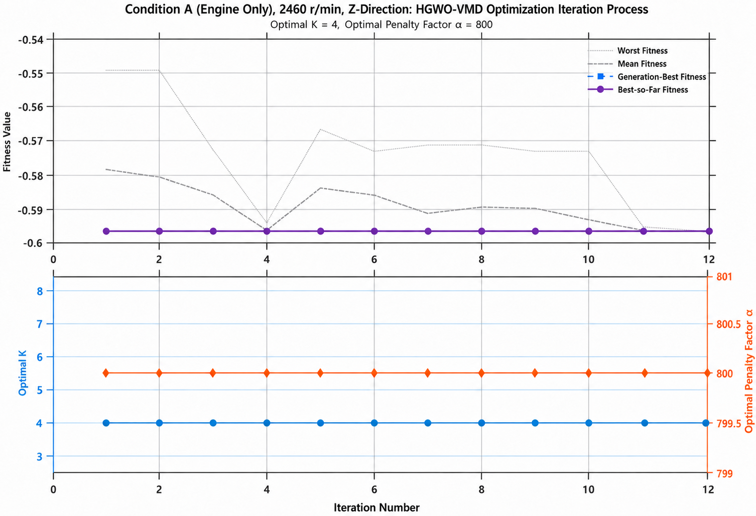
The iteration results of the adaptive mode number and penalty factor optimization based on HGWO–VMD are shown in Figure 17.

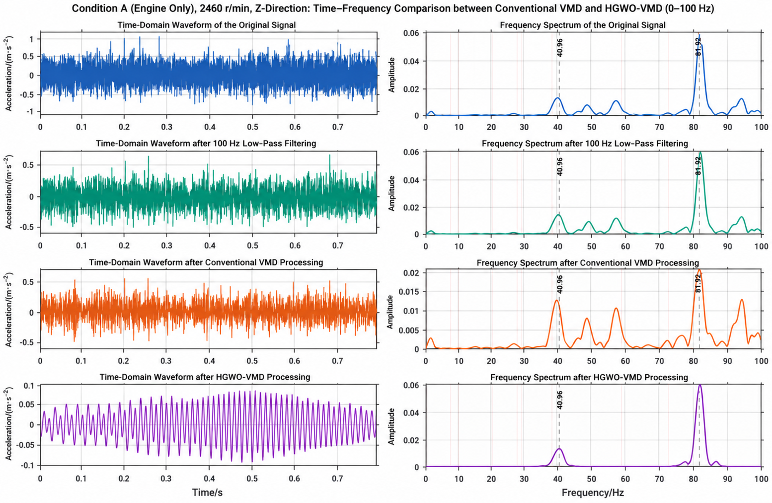
The optimization yielded a mode number of K = 4 and a penalty factor of α = 800. VMD with these two parameters was used to process the Z–direction vibration signal of the cab under Condition A, and the results were compared with the original signal, the low-pass filtered signal, and the conventional VMD–processed signal in the time and frequency domains, as shown in Figure 18.

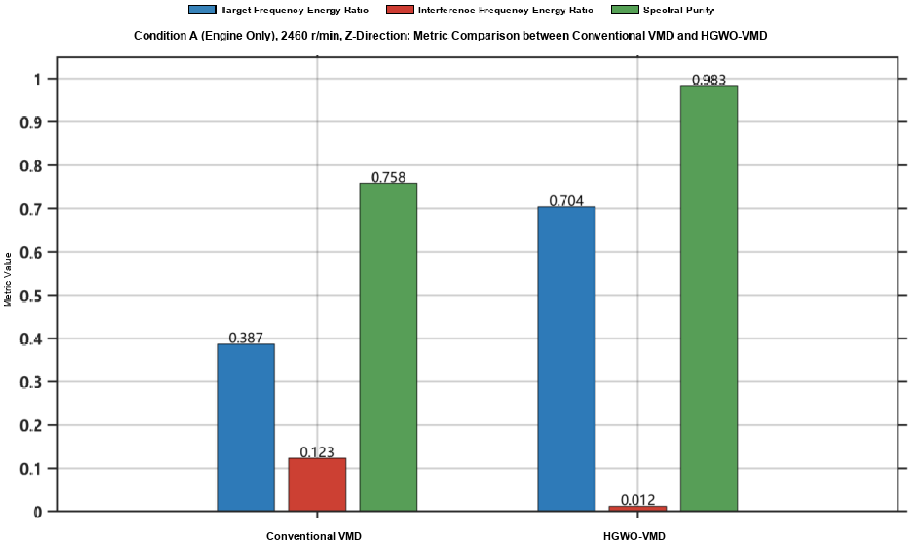
Under Condition A, the Z–direction spectrum contains components at 40.96, 81.92 and 58.88 Hz (Figure 18). The first two are consistent with engine rotation and second-order excitation. The component at 58.88 Hz may be associated with the dynamic response of the cab system. Conventional VMD attenuates the 81.92 Hz component, whereas the HGWO–VMD reconstruction retains prominent components near 40.96 and 81.92 Hz. Figure 19 compares their frequency–band energy metrics.

The results show that the target-frequency energy ratio of conventional VMD is only 0.387, the interference-frequency energy ratio reaches 0.123 and the spectral purity is 0.758. For the HGWO–VMD processing chain, the target-frequency energy ratio increases to 0.704, the interference-frequency energy ratio decreases to 0.012 and the spectral purity reaches 0.983.

3.2.4. Vibration Signal Analysis of the Cab in the X Direction Under Condition B

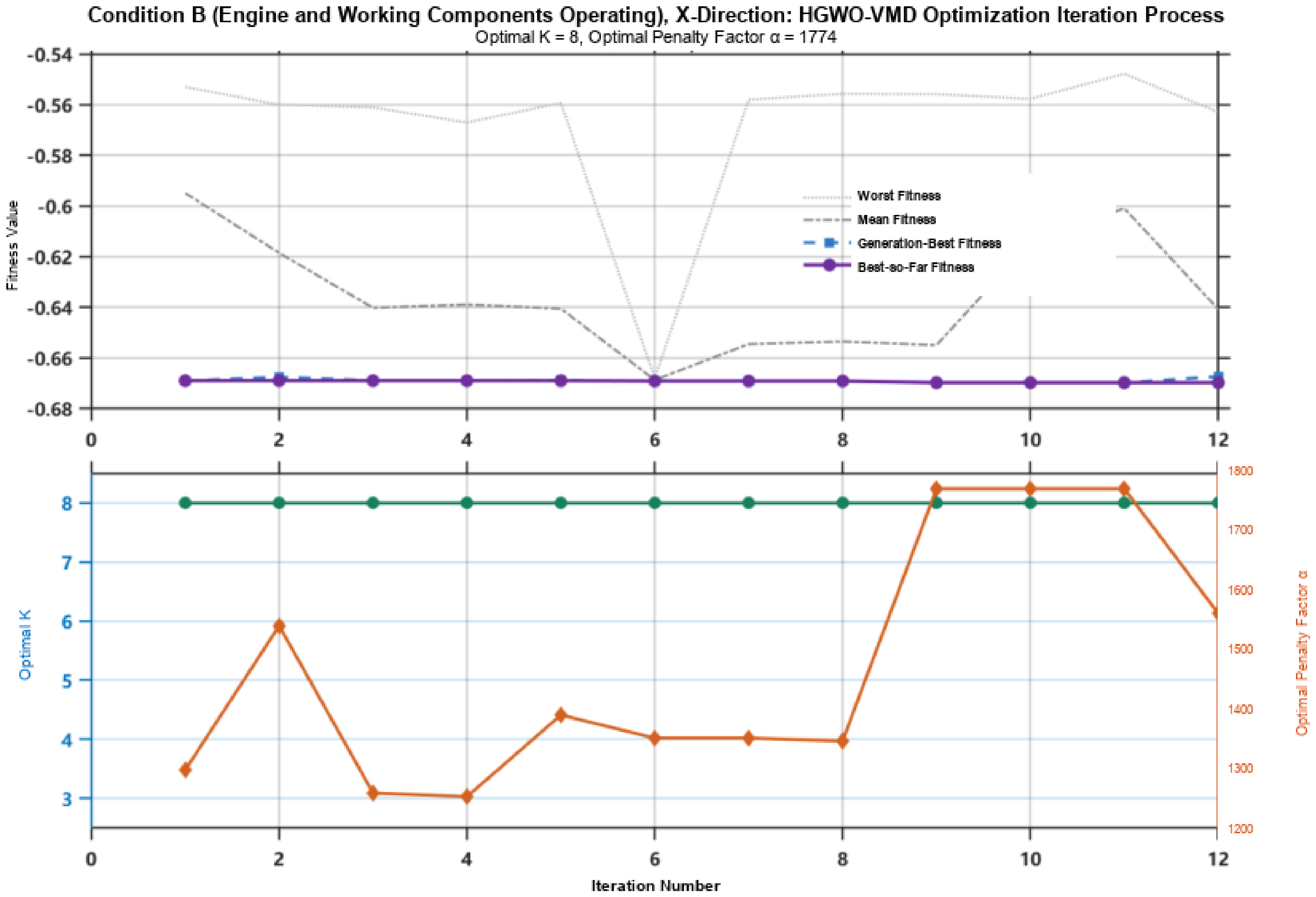
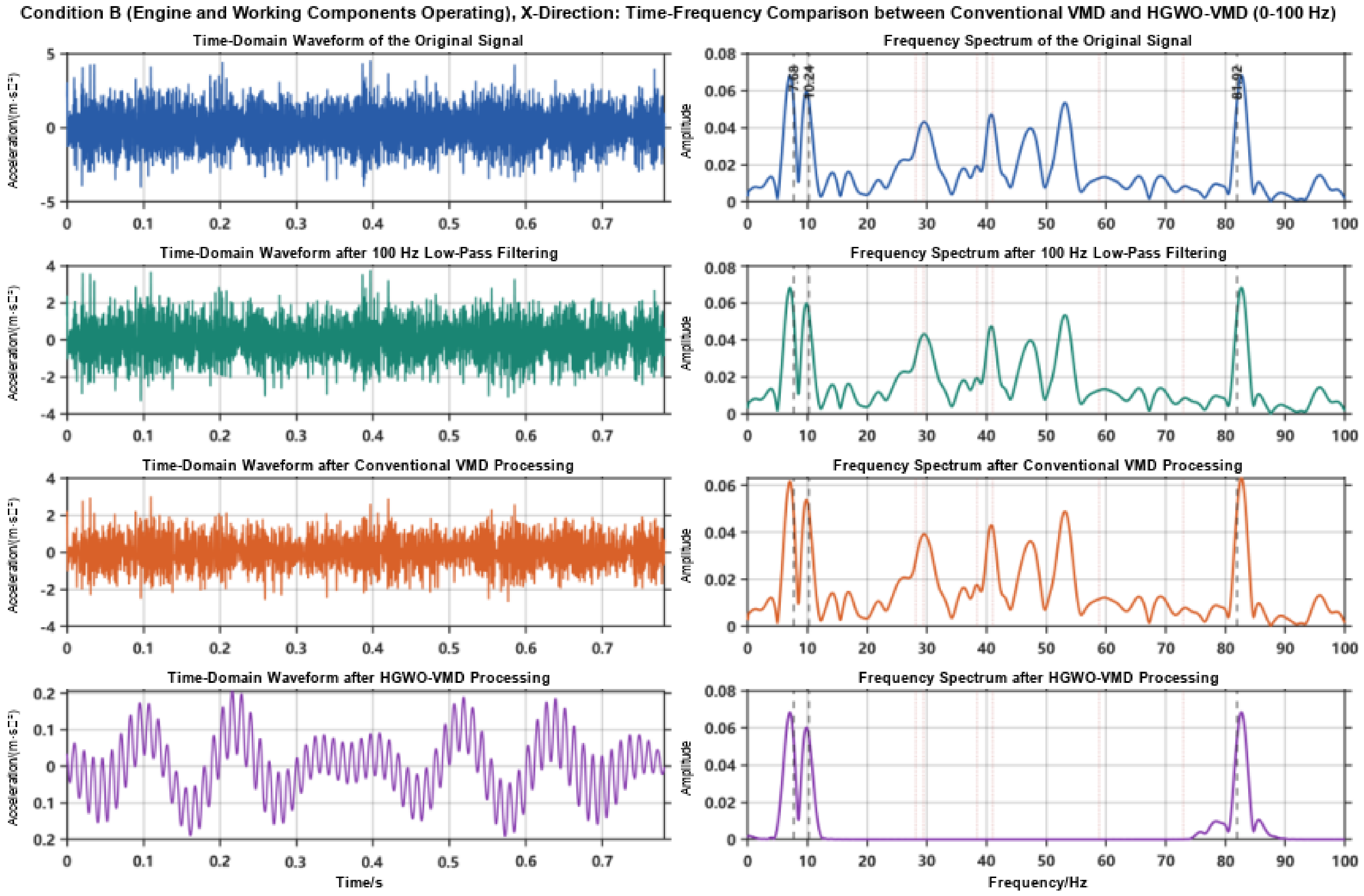
For the X–direction signal under Condition B, the single optimization run yielded K = 8 and α = 1774 (Figure 20). VMD with this parameter pair was compared with the original signal, the low-pass-filtered signal and the conventional VMD reconstruction (Figure 21).

Under Condition B, multiple working components operate simultaneously. Figure 21 shows prominent components near 81.92, 7.68 and 10.24 Hz in the HGWO–VMD reconstruction. The 10.24 Hz component falls within the measured cutter rotational frequency range of 9.25–10.58 Hz and was not observed under Condition A; it is therefore consistent with cutter operation. Components near 81.92 and 7.68 Hz are consistent with engine second-order excitation and vibrating screen operation, respectively. The spectra differ in their additional components within 20–60 Hz, but this comparison does not establish that all excluded components are noise or that mode mixing is eliminated.

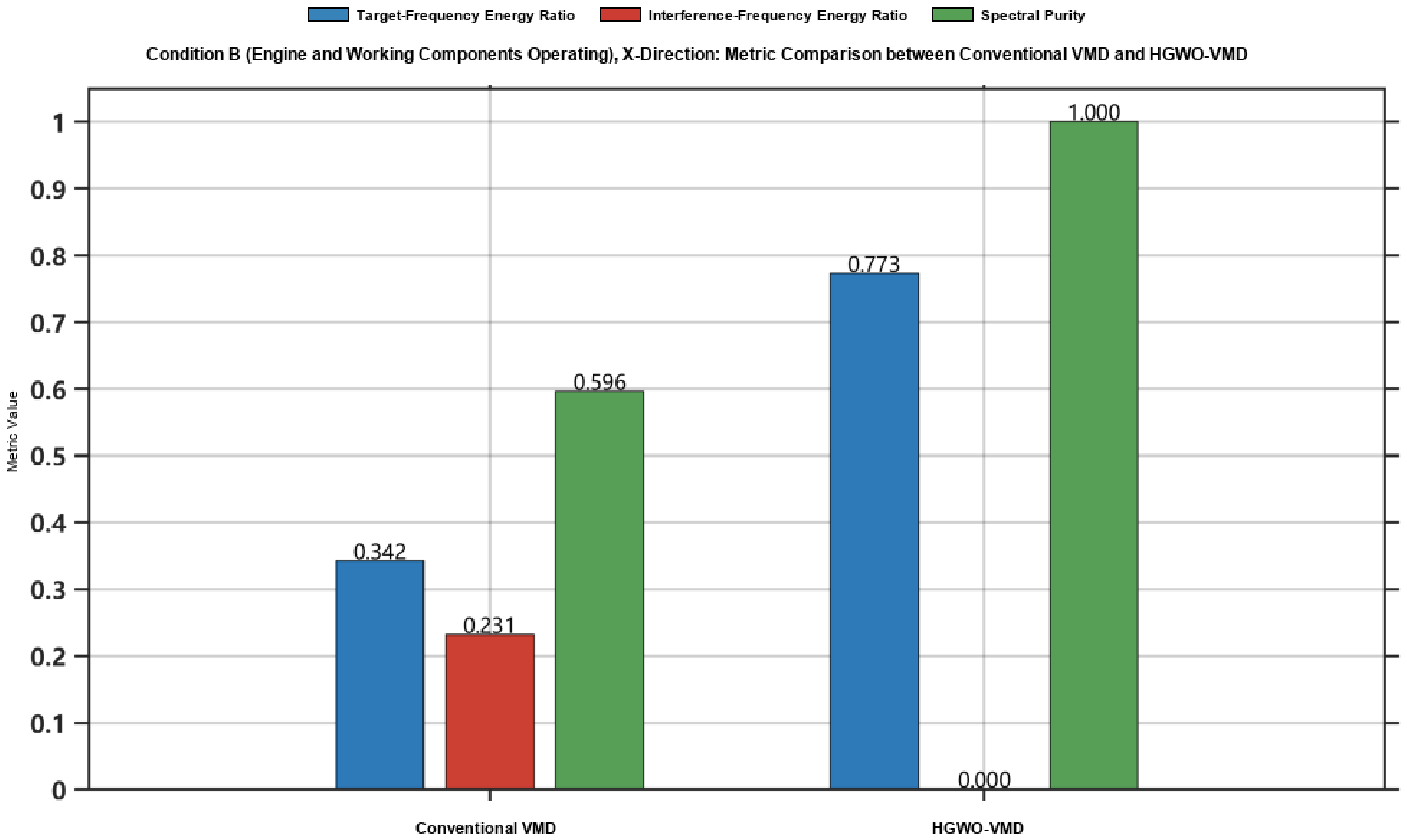
For the X–direction signal under Condition B (Figure 22), conventional VMD gives R_T = 0.342, R_I = 0.231 and η = 0.596. HGWO-VMD gives R_T = 0.773, R_I close to zero and η close to 1. The comparison indicates an increased energy proportion in the selected target bands for the analyzed record.

3.2.5. Vibration Signal Analysis of the Cab in the Y Direction Under Condition B

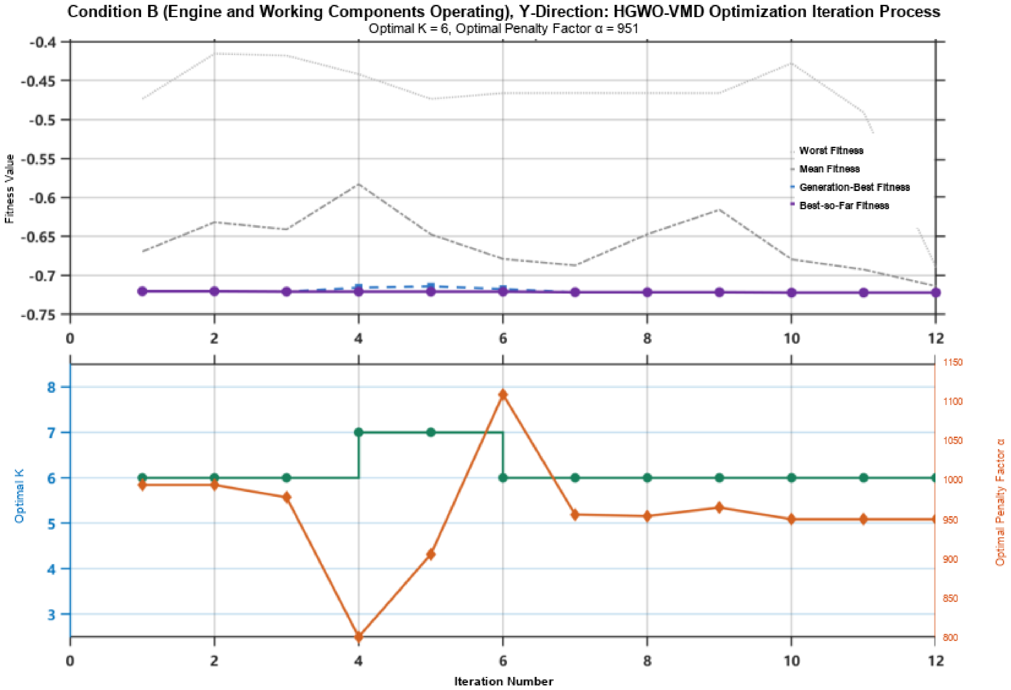
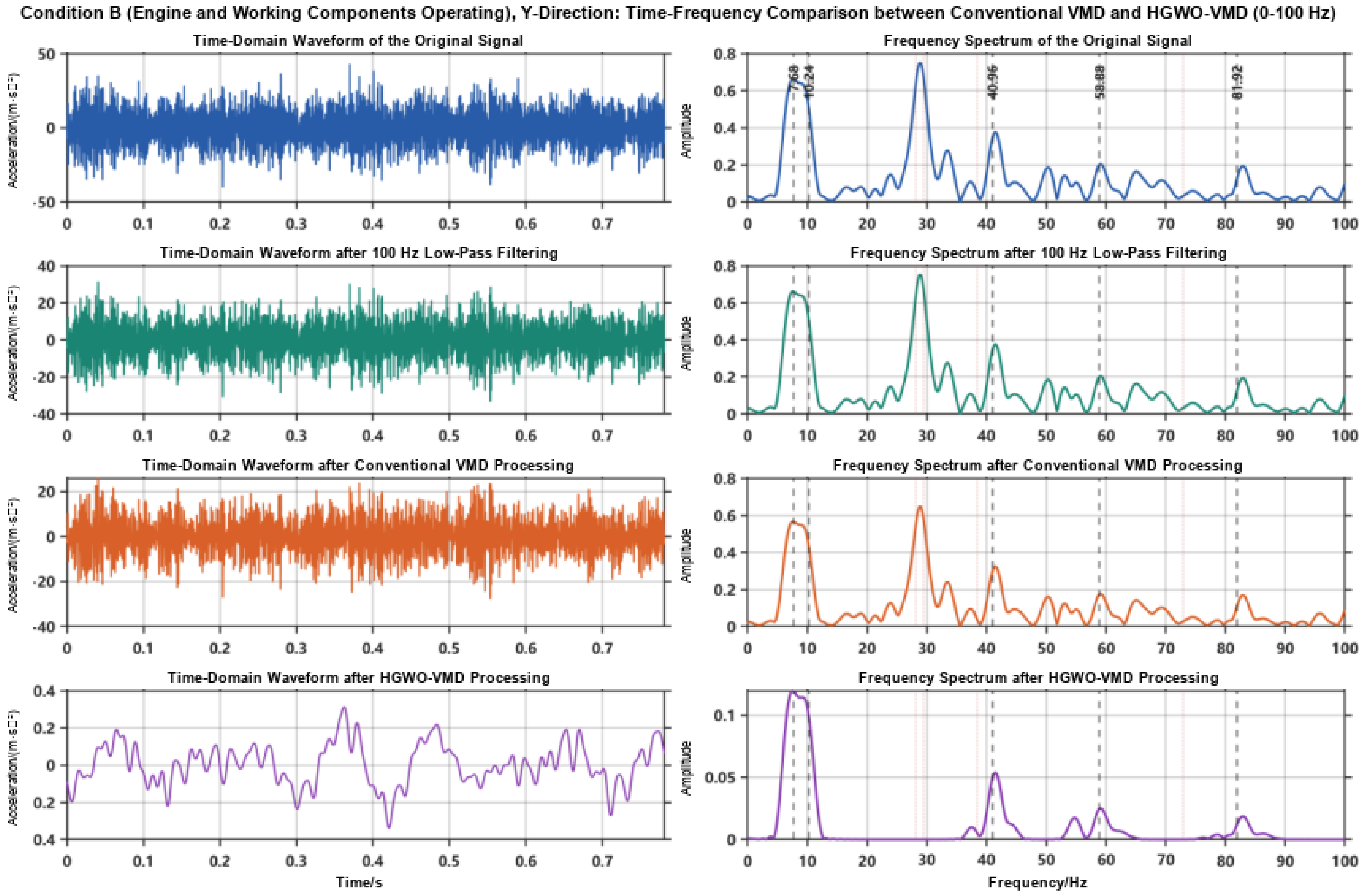
The optimization iteration results of the mode number and penalty factor for the Y–direction cab vibration signal under Condition B are shown in Figure 23. The optimization yielded a mode number of K = 6 and a penalty factor of α = 951. VMD with the optimized parameters was used to process the Y-direction vibration signal under Condition B, and the results were compared with the original signal, the low-pass filtered signal, and the conventional VMD-processed signal in the time and frequency domains, as shown in Figure 24.

The Y–direction spectra under Condition B contain components near 7.68, 10.24, 40.96 and 82–83 Hz, consistent with vibrating screen operation, cutter operation, engine rotation and engine second-order excitation, respectively (Figure 24). The 29.44 Hz component is attenuated in the HGWO–VMD reconstruction. A low-amplitude component at 58.88 Hz remains and also occurs under Condition A. It may be associated with the dynamic response of the cab system; its presence does not establish a specific coupling resonance.

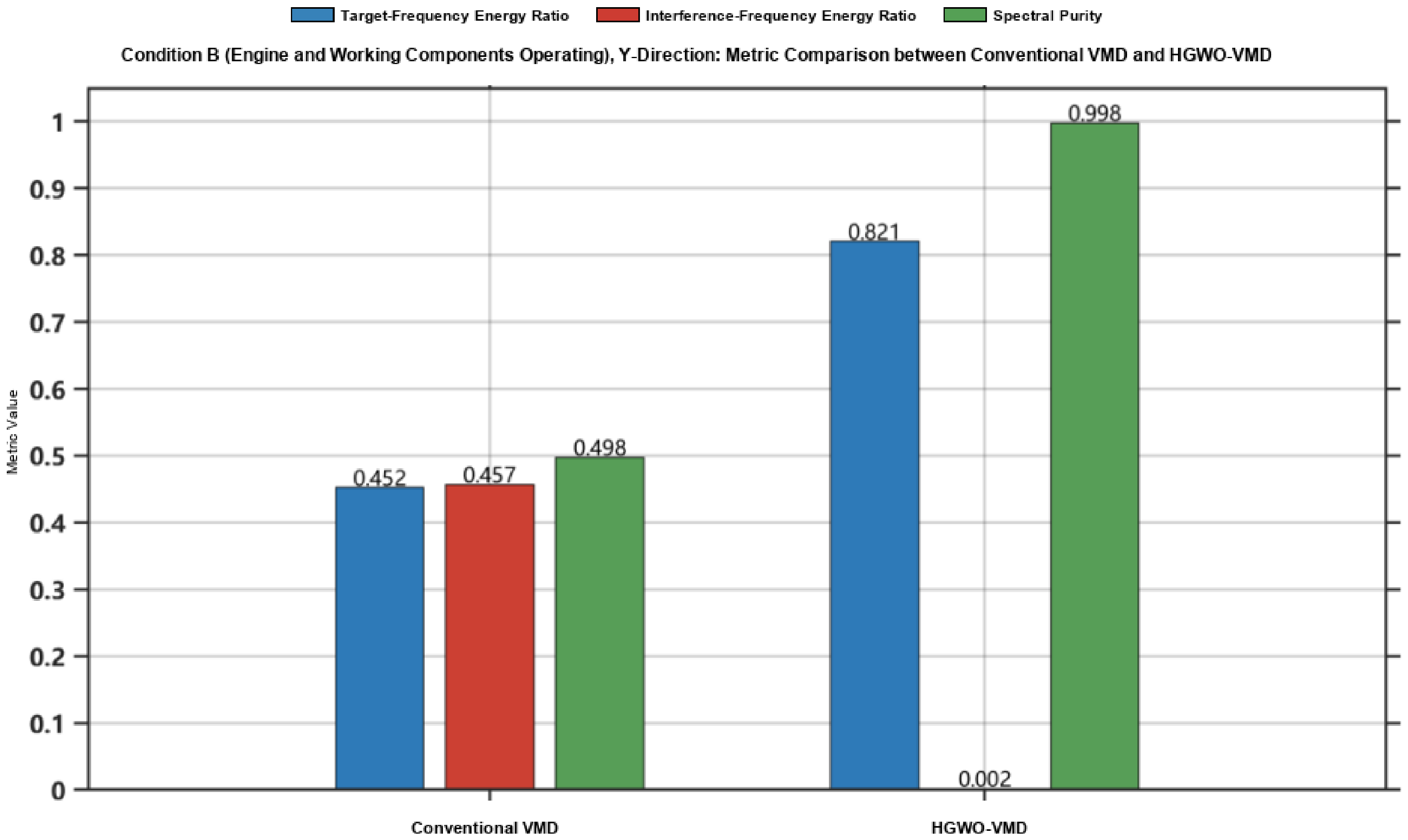
The energy ratio and purity comparison of each frequency in the signal are shown in Figure 25. The results show that the target-frequency energy ratio of conventional VMD is only 0.452, the interference-frequency energy ratio reaches 0.457 and the spectral purity is only 0.498. For the HGWO-VMD processing chain, the target-frequency energy ratio increases to 0.821, the interference-frequency energy ratio decreases to 0.002 and the spectral purity reaches 0.998.

3.2.6. Vibration Signal Analysis of the Cab in the Z Direction Under Condition B

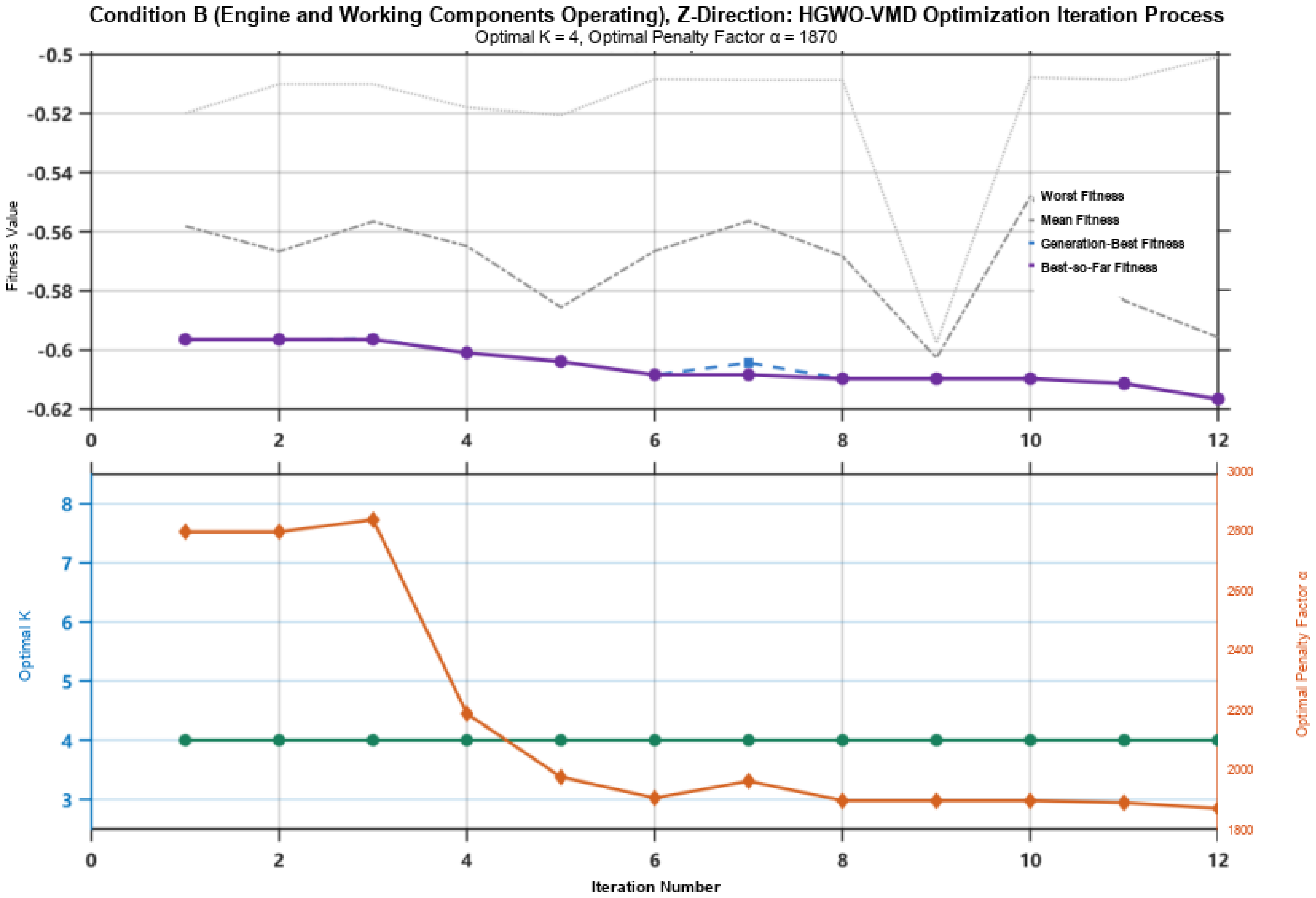
The optimization iteration results of the mode number and penalty factor for the Z–direction cab vibration signal under Condition B are shown in Figure 26. The optimization yielded a mode number of K = 4 and a penalty factor of α = 1870. VMD with the optimized parameters was used to process the Z-direction vibration signal under Condition B, and the results were compared with the original signal, the low-pass filtered signal and the conventional VMD-processed signal in the time and frequency domains, as shown in Figure 27.

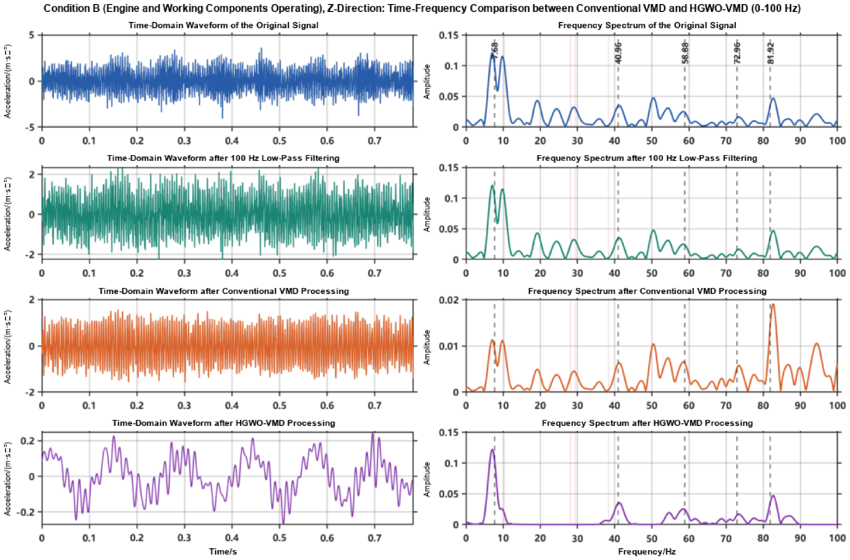
Under Condition B, the Z–direction signal contains several closely spaced low–frequency components (Figure 27). Conventional VMD changes the RMS from 0.9238 to 0.0227 m/s². This is a signal–processing result rather than mechanical vibration reduction. Components near 7.68, 10.24, 40.96 and 81.92 Hz remain visible, together with additional content near 58.88 and 72.96 Hz.

After HGWO–VMD processing, the principal components near 7.68, 10.24, 40.96 and 81.92 Hz remain visible. The 72.96 Hz component falls within 69.0–73.0 Hz, the sixth–order range corresponding to the measured threshing drum speed of 690–730 r/min, and is consistent with sixth–order drum excitation. The spectrum also contains a component at 58.88 Hz, which may be associated with the dynamic response of the cab system.

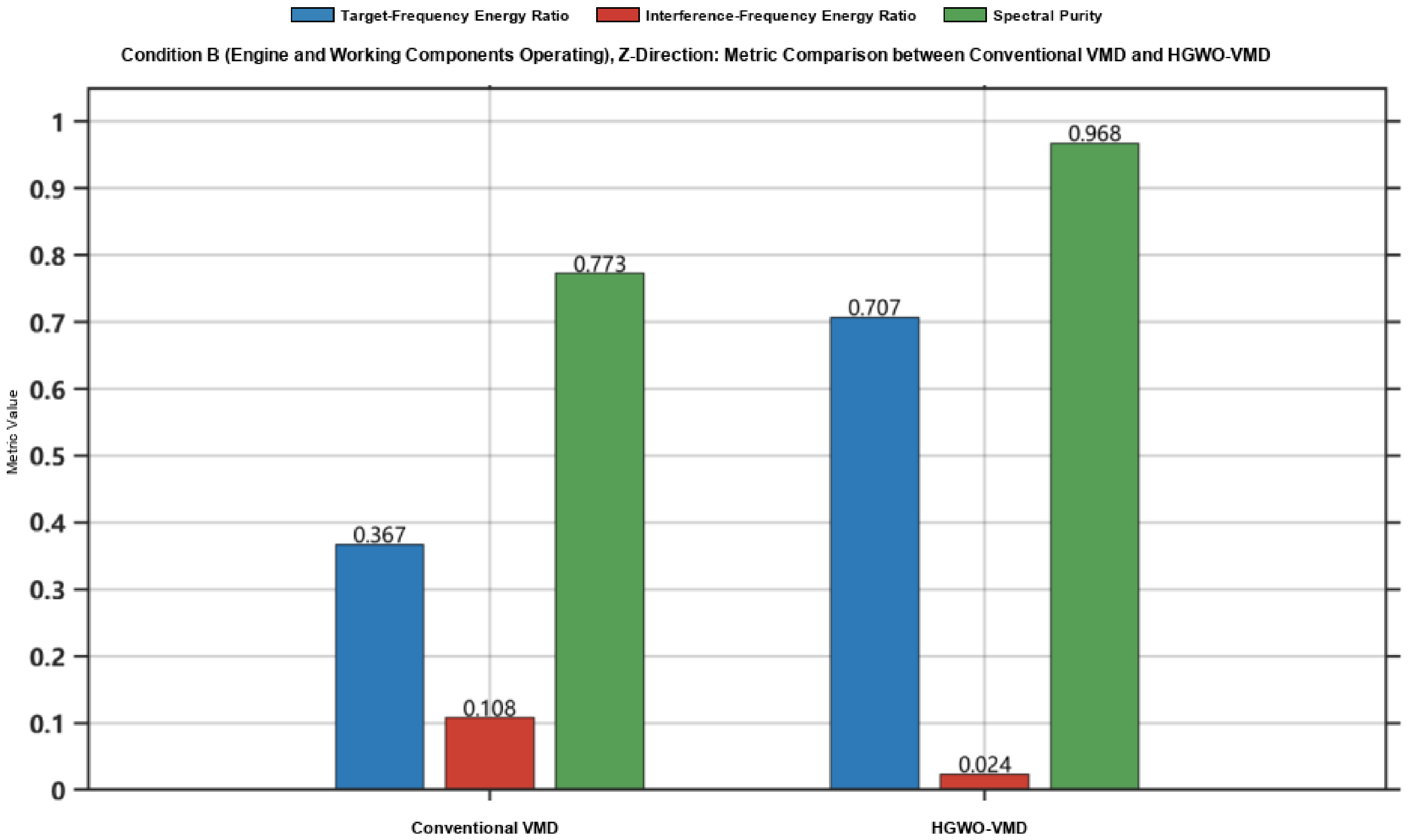
The energy ratio and spectral purity comparison of each frequency in the signal are shown in Figure 28. For conventional VMD, the target-frequency energy ratio is 0.367, the interference-frequency energy ratio reaches 0.108 and the spectral purity is 0.773. For the HGWO-VMD processing chain, the target-frequency energy ratio increases to 0.707, the interference-frequency energy ratio decreases to 0.024 and the spectral purity reaches 0.968. The feature frequencies extracted from the original cab vibration signal under Condition B by conventional VMD and HGWO–VMD are summarized in

Table 3. Comparison of the feature frequency extraction results between VMD and HGWO–VMD under Condition B.

Axis	Conventional VMD (Hz)	HGWO-VMD (Hz)	Vibration Features After HGWO-VMD	Possible Source
X	81.92, 7.68, 10.24, 58.88, 29.44, 40.96, additional components	81.92, 7.68, 10.24	E2; VS; C	Engine; screen; cutter
Y	83.2, 58.88, 40.96, 29.44, 10.24, 7.68, additional components	83.2, 58.88, 40.96, 10.24, 7.68	E1; E2; AR; C; VS	Engine; cutter; screen
Z	81.92, 72.96, 58.88, 7.68, 29.44, 40.96, 10.24, additional components	81.92, 72.96, 58.88, 7.68, 40.96	E1; E2; T6; AR; VS	Engine; drum; screen

Abbreviations: E1, engine rotation; E2, engine second-order excitation; VS, vibrating screen rotation; C, cutter rotation; T6, sixth-order drum excitation; AR, additional response component. These are frequency correspondences rather than independently verified source assignments.

.

Table 3 summarizes the reported frequencies under Condition B. In the X direction, the main HGWO-VMD components are 7.68, 10.24 and approximately 82–83 Hz; the Y– and Z–direction results also contain a component near 40.96 Hz. The component near 72.96 Hz in the Z direction is consistent with sixth-order threshing drum excitation. A component at 58.88 Hz is observed in the Y and Z directions and may be associated with the dynamic response of the cab system. These frequency correspondences guide the choice of mechanical modifications without confirming individual transfer paths.

4. Targeted Vibration Reduction Optimization Design Based on Feature Frequency Identification

The observed cab vibration frequencies and their possible associations with operating components are summarized in

Table 4. Feature frequencies and excitation components causing the three-directional cab vibration.

Condition and Direction	Typical Feature Frequencies (Hz)	Frequency Correspondence
A-X	81.92, 40.96	Engine second harmonic f2f, fundamental f1f
A-Y	81.92, 40.96	Engine second harmonic f2f, fundamental f1f
A-Z	81.92, 40.96	Engine second harmonic f2f, fundamental f1f
B-X	81.92, 7.68, 10.24	Engine second harmonic f2f, cutter fundamental f1q, vibrating screen fundamental f1z
B-Y	81.92, 58.88, 40.96, 10.24, 7.68	Engine second harmonic f2f and fundamental f1f, vibrating screen fundamental f1z, additional cab response component, cutter fundamental f1q
B-Z	81.92, 72.96, 58.88, 7.68, 40.96	Engine second harmonic f2f and fundamental f1f, vibrating screen fundamental f1z, additional cab response component, threshing drum sixth harmonic f6t

. These correspondences were used to guide mechanical modifications.

The observed components near 40.96 Hz and 82–83 Hz are consistent with engine rotation and second-order excitation. Under Condition B, components near 7.68 and 10.24 Hz are consistent with vibrating screen and cutter operation, and 72.96 Hz is consistent with sixth-order threshing drum excitation. The 58.88 Hz component may be associated with the dynamic response of the cab system. The implemented measures were vibrating screen counterweight balancing, cutter speed adjustment combined with counterweight balancing, and inclined cab supports. Subsequent vibration tests compared the effects of different combinations of these measures.

4.1. Vibrating Screen Modal Analysis and Counterweight Balancing

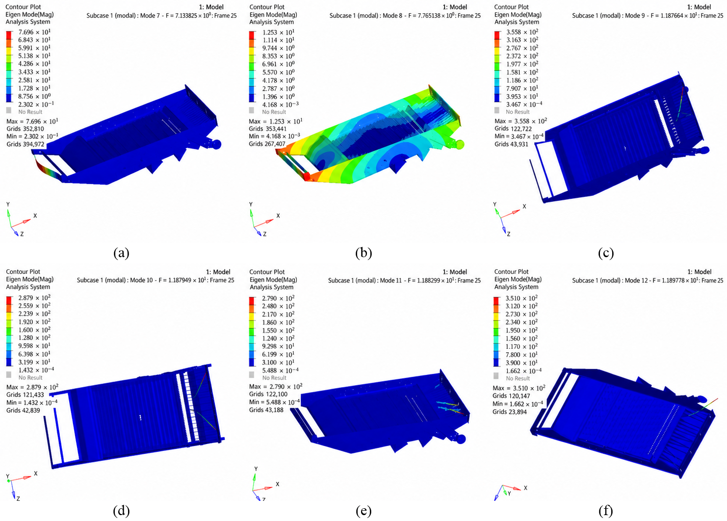
A finite element model of the vibrating screen was constructed in HyperMesh 2022 and solved using OptiStruct 2022. Bolts and other assembly parts were removed while the screen body was retained. The screen body was made of Q235 steel, with nominal material properties of elastic modulus E = 206 GPa, Poisson’s ratio ν = 0.30, and density ρ = 7850 kg/m³. The mesh consisted mainly of shell elements assigned PSHELL properties, with a small number of solid elements assigned PSOLID properties; element sizes were 2–4 mm. Welded connections were represented using RBE3 couplings. Both ends of the screen were fixed. Figure 29 and

Table 5. First six calculated elastic natural frequencies of the vibrating screen.

Order	1	2	3	4	5	6
Frequency/Hz	7.1	7.7	11.86	11.88	11.95	11.98

show the first six calculated elastic modes and their natural frequencies under these model conditions.

Figure 29 shows front-end bending in the first mode, combined bending and torsion in the second mode, and more localized bending and torsional deformation in the higher modes. The measured screen operating frequency range of 6.93–7.93 Hz is close to the first two calculated natural frequencies, 7.1 and 7.7 Hz. This proximity suggests the possibility of amplified vibration response. A component at 7.68 Hz was observed in the cab signals.

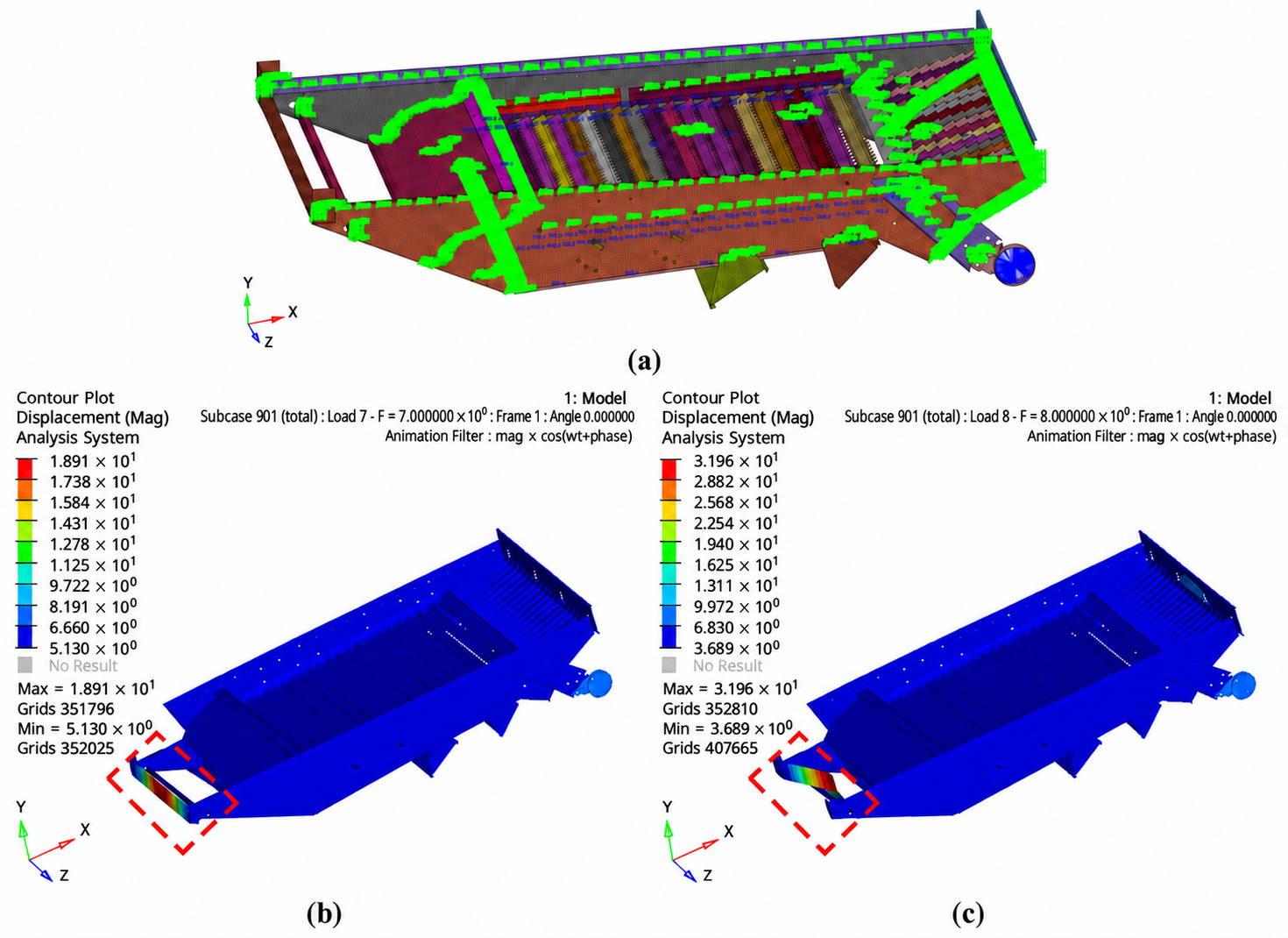
Figure 30 presents forced harmonic responses calculated at 7 and 8 Hz. No damping was specified. The excitation amplitude was calculated from the unbalanced inertia force of the crank-rocker mechanism at the corresponding speed for each calculation. The load was applied at the screen drive-wheel center, coupled to the surrounding structure using RBE2 elements, with upward vertical motion defined as the positive force direction. The maximum displacements were 18.89 mm at 7 Hz and 31.96 mm at 8 Hz. These are forced-response displacements under the stated loads and constraints, not modal display amplitudes. Both the different force amplitudes and the structural frequency response affect the comparison. The 8 Hz point was an analysis frequency slightly above the measured operating range; the two calculations do not define a resonance bandwidth.

The screen excitation originates from the unbalanced inertia force generated by the crank-rocker mechanism. The simplified force calculation includes rotating and reciprocating inertia terms. Counterweight balancing was considered to reduce the unbalanced force. The centrifugal inertia force is:

$$F_{\mathrm{ql}}=m_{\mathrm{ql}}r{{\omega }_2}^2$$

(27)

Here, m_ql is the equivalent rotating mass of the screen crank, r is the crank radius, and ω₂ is the crank angular velocity in rad/s.

The simplified engineering expression of the reciprocating inertial force is:

$$F_{\mathrm{qw}}=m_{\mathrm{qw}}{\alpha }_{\mathrm{qw}}$$

(28)

Here, m_qw is the equivalent reciprocating mass, α_qw is the reciprocating acceleration in the simplified model, θ is the crank angle, λ₁ is the connecting-rod ratio, and l is the connecting-rod length. The acceleration and force terms are evaluated using the stated kinematic relations.

Therefore, the total unbalanced force F_un is:

$$F_{\mathrm{un}}=F_{\mathrm{ql}}+F_{\mathrm{qw}}$$

(29)

To reduce the vibration caused by the unbalanced force, a counterweight mb can be added on the symmetric side of the crank to balance the centrifugal force:

$${\mathrm{m}}_b{r}_b{{\omega }_2}^2=m_{\mathrm{q}1}r{{\omega }_2}^2$$

(30)

where r_b is the radius of the added counterweight.

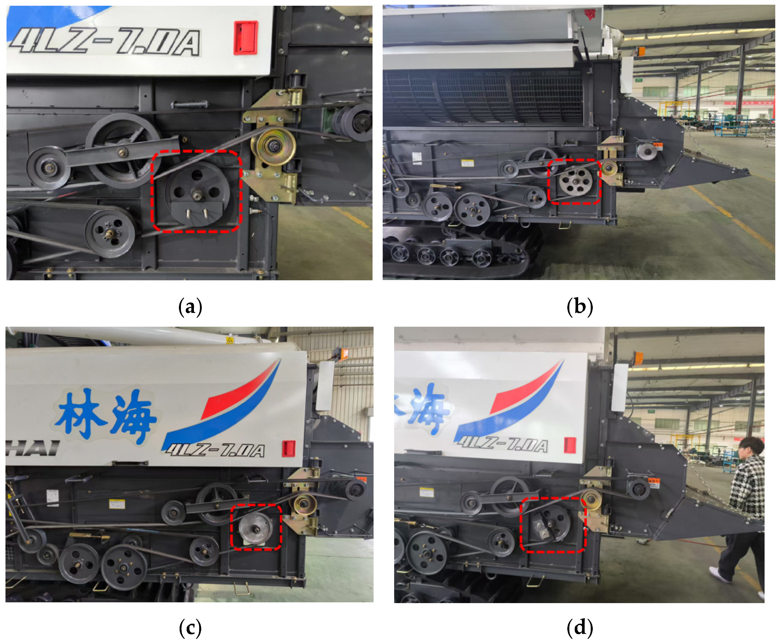
The parameters of the crank-rocker mechanism of the vibrating screen are listed in

Table 6. Parameters of the crank-rocker mechanism of the vibrating screen of the Linhai 4LZ-7A combine harvester.

Parameter	Value
mql	6 kg
r	0.04 m
${\omega }_2$	46 rad/s
mqw	2 kg
αqw	[−81, 88] m/s2
λ1	0.042
l	0.3 m
rb	0.1 m

. Calculations show that the counterweight mb on the symmetric side of the crank-rocker mechanism of the vibrating screen should be 2.4 kg. In addition, the outer diameter of the drive pulley of the vibrating screen of the Linhai 4LZ-7A combine harvester is 225 mm. When the external excitation frequency is changed for vibration reduction, the current drive speed of the vibrating screen is 450 r/min and the intermediate shaft speed is 918 r/min; the initial transmission ratio i1 of the vibrating screen is:

$$i_1={\displaystyle \frac{n_{\mathrm{S}}}{n_P}}={\displaystyle \frac{D_P}{D_S}}={\displaystyle \frac{\phi 110}{\phi 225}}=0.49$$

(31)

where $n_{\mathrm{S}}$ is the vibrating screen speed and $n_P$ is the intermediate shaft speed.

Two pulley-speed alternatives were considered: 405 and 480 r/min, corresponding to 6.75 and 8 Hz. The associated transmission ratios are:

$$i_{1\text{-}1}={\displaystyle \frac{n_{\mathrm{S}}}{n_P}}=0.45={\displaystyle \frac{\phi 110}{\phi 243}}$$

(32)

$$i_{1\text{-}2}={\displaystyle \frac{n_{\mathrm{S}}}{n_P}}=0.53={\displaystyle \frac{\phi 110}{\phi 205}}$$

(33)

Calculations show that the outer diameters of the drive pulley corresponding to the reduced-speed ratio i_1-1 and the increased-speed ratio i_1-2 are 243 mm and 205 mm, respectively. The vibration reduction optimization scheme of the vibrating screen drive system is shown in Figure 31.

The pulley-diameter adjustment alternatives were analyzed but were not adopted in the final vibration reduction tests. Their calculated operating frequencies, 6.75 and 8 Hz, remained close to the relevant natural frequencies. The implemented screen modification was counterweight balancing.

4.2. Cutter Speed Adjustment and Counterweight Balancing

The cutter of the Linhai 4LZ-7A combine harvester also performs reciprocating motion driven by a crank-rocker mechanism, generating vibration that is transmitted to the cab [13]. When the counterweight method is used for the vibration reduction optimization of the cutter and its transmission system, the required counterweight mass is calculated with reference to Equations (27)–(30). The parameters of the cutter crank-rocker mechanism are listed in

Table 7. Parameters of the cutter crank-rocker mechanism.

Parameter	Value
mq2	1.2 kg
rq	16 mm
${\omega }_3$	60 rad/s
mqw1	1 kg
αqw1	[−84.3, 95.7] m/s2
λ2	0.063
l1	400 mm
rb1	25 mm

.

For the cutter, m_q2 is the equivalent rotating crank mass, r_q is the crank radius, and ω is the angular velocity in rad/s. The symbols m_qw1 and α_qw1 denote the equivalent reciprocating mass and acceleration, θ is the crank angle, λ₂ is the connecting-rod ratio, l₁ is the connecting-rod length, and r_b1 is the counterweight radius.

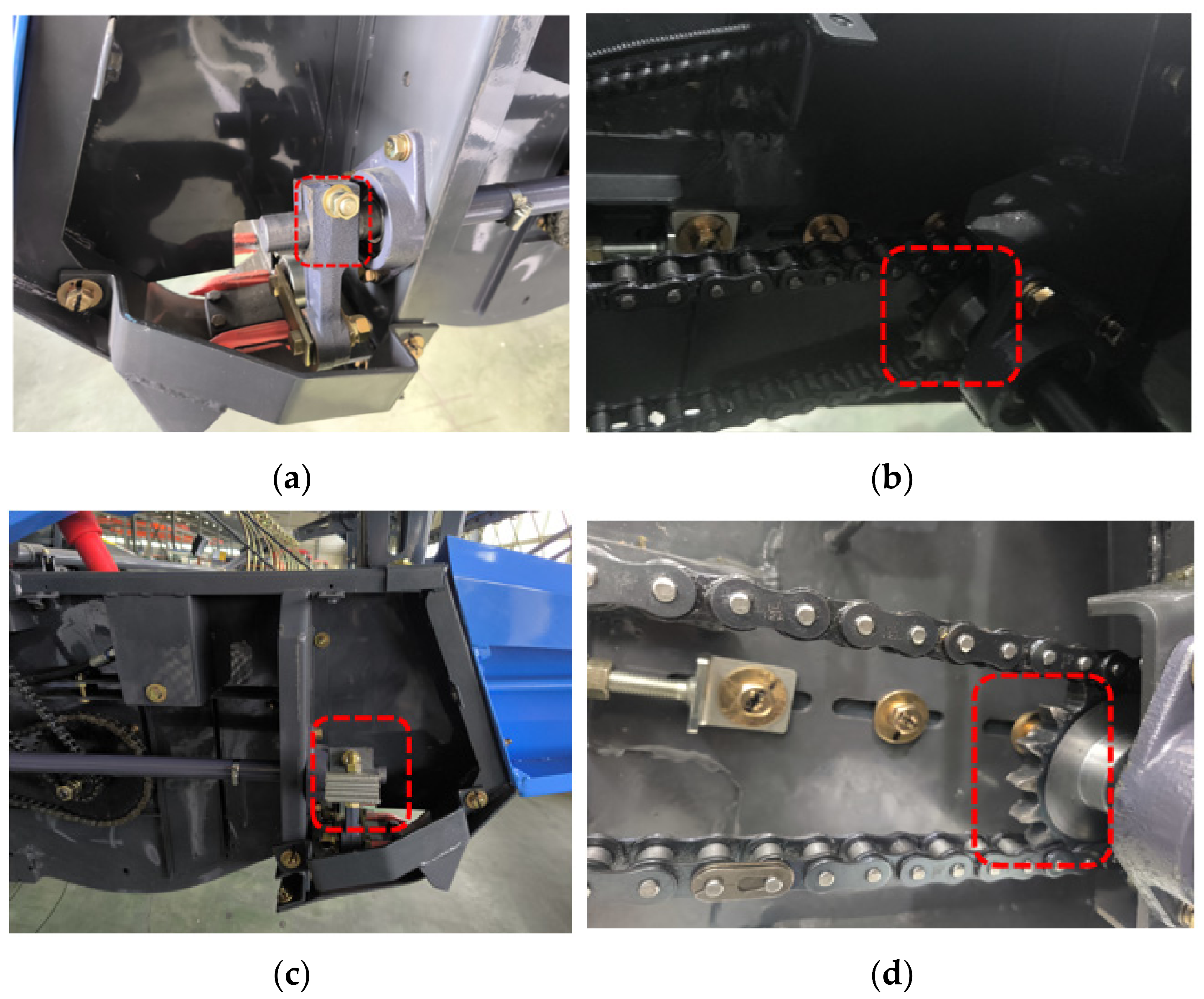
The calculated cutter counterweight was 768 g, and 750 g was used in practice. The original cutter drive sprocket had 16 teeth, the speed was 580 r/min and the transmission ratio was 1.125. Replacing the sprocket with 17 teeth changed the speed to 544 r/min (approximately 9 Hz) and the transmission ratio to 1.058. This speed adjustment was combined with counterweight balancing (Figure 32). The combined measures were evaluated through stationary no-load vibration tests. Field cutting performance at 544 r/min was not tested, so preservation of cutting efficiency or crop-cutting quality is not claimed.

4.3. Vibration Reduction Optimization Design of the Cab Based on Inclined Support Mounting with Vibration Decomposition

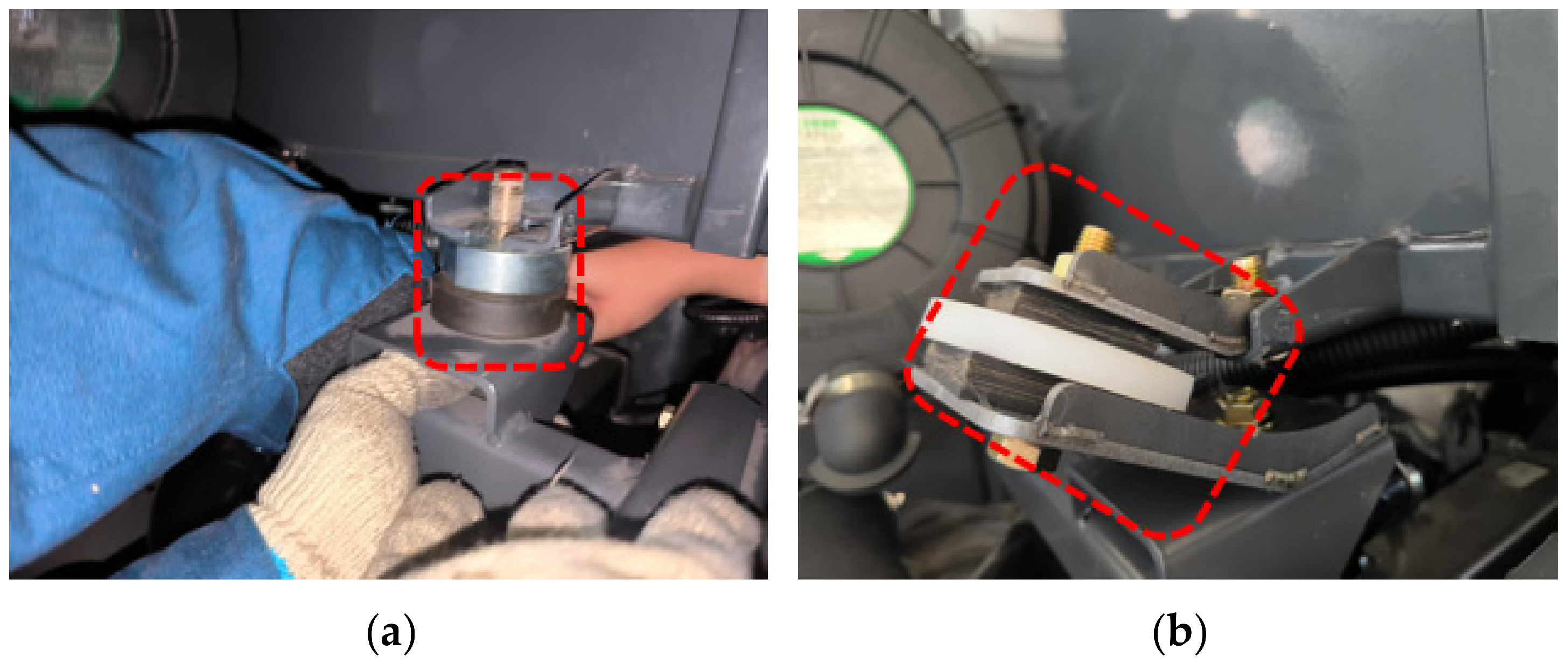
The cab-to-beam supports were redesigned with an inclined configuration (Figure 33). Q355 steel supports with inclinations of 30°, 45° and 60° were considered and tested in preliminary vibration measurements, but the corresponding comparative results were not retained. The 30° configuration was adopted for the subsequent combined vibration reduction tests; it is not presented as an experimentally established optimum among the three angles.

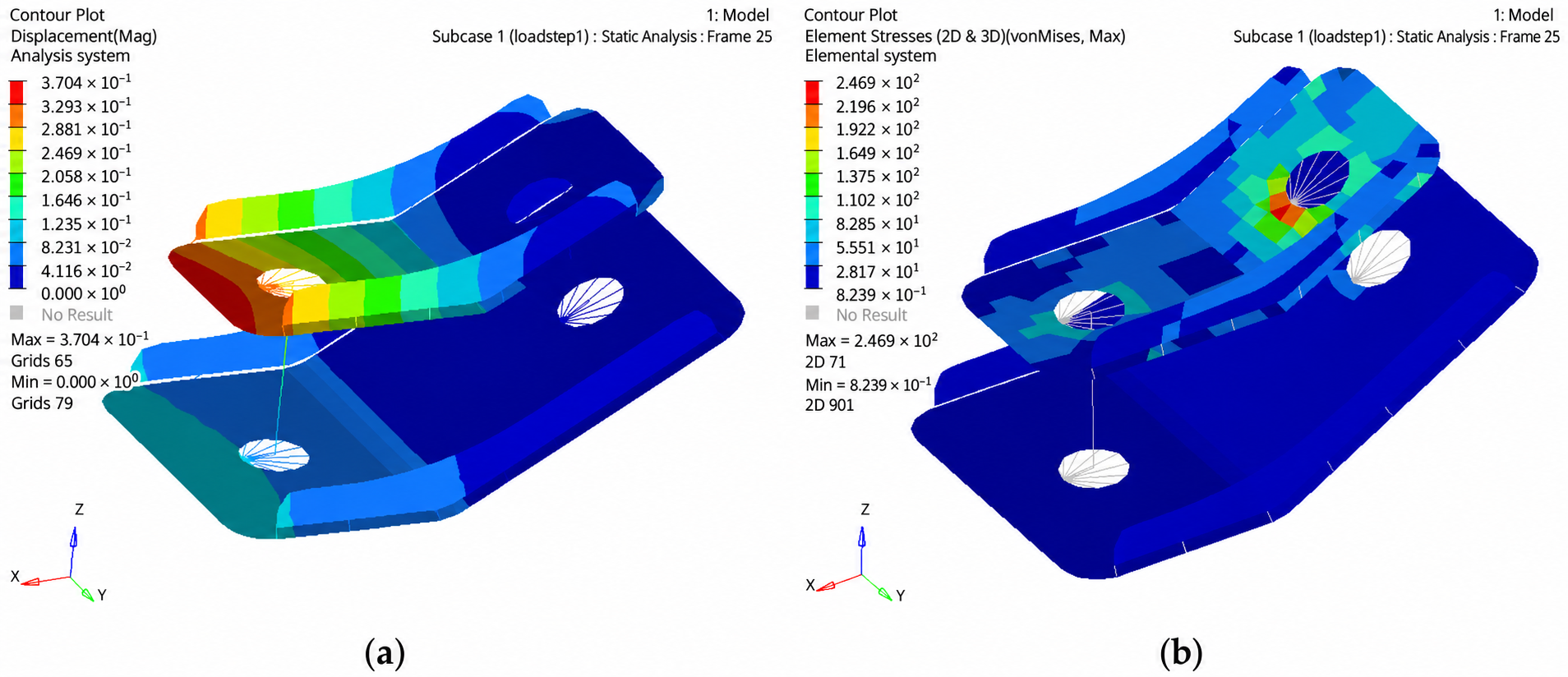
A static analysis was carried out to check support strength under the applied weight loads of the cab and occupant. Bolted connections were represented by constraints, and the vibration damping pad was represented using CBUSH elements. Figure 34 shows the calculated static deformation and stress of the 30° support. This check addresses the specified static load case and is not a fatigue or durability assessment.

The calculated static displacement of the 30° support was 0.37 mm (Figure 34a). The maximum stress was 247 MPa at the upper support connection; applying the stated factor of 1.2 gives approximately 297 MPa, below the 355 MPa strength criterion used in the analysis (Figure 34b). The support satisfied this static strength check. These results do not establish fatigue life or long-term durability.

4.4. Test Results and Analysis of the Targeted Vibration Reduction

The implemented combinations were evaluated on the same harvester under Condition B. Directional acceleration RMS values and their three-axis resultant were calculated for the cab and header before and after modification. Each

Table 8. Directional and overall acceleration RMS values (m/s²) for the tested header and cab modification combinations.

Scheme	Combination	H-X (m/s2)	H-Y (m/s2)	H-Z (m/s2)	H-All (m/s2)	C-X (m/s2)	C-Y (m/s2)	C-Z (m/s2)	C-All (m/s2)
Baseline	Original harvester	3.83	5.14	5.09	8.18	1.37	1.71	10.59	10.82
Scheme 1	OA + OB + OC	2.55	5.21	4.41	7.28	1.22	3.32	5.36	6.42
Scheme 2	OA + OB + OD	2.58	5.24	4.5	7.40	1.10	3.37	4.45	5.68
Scheme 3	OA + OB + OD + OE	2.66	5.08	4.45	7.25	1.22	3.41	5.11	6.26
Scheme 4	OA + OB + OD + OF	2.62	4.99	4.45	7.18	1.07	3.39	4.32	5.59

Note: OA, replacing the cutter sprocket with 17 teeth; OB, inclined cab support; OC, 300 g counterweight on the vibrating screen pulley; OD, 2.4 kg counterweight on the vibrating screen pulley; OE, 500 g counterweight on the cutter arm; OF, 750 g counterweight on the cutter arm. All RMS values are in m/s² and were calculated over 20 s. The reported reductions compare the single recorded result for each configuration with the baseline. H denotes the header, C denotes the cab, and all denotes the three-axis resultant RMS. The overall RMS is a_v = √(a_x² + a_y² + a_z²), where a_x, a_y and a_z are the directional acceleration RMS values. All directional coefficients are 1, and no human-vibration frequency weighting was applied.

value was calculated from a 20 s segment of a single measurement record, not from an average of independent repeated measurements. No human-vibration frequency weighting was applied, and the directional coefficients were all 1. The overall value was calculated as the square root of the sum of the squared directional RMS values. Table 8 compares the tested combinations; it does not isolate the contribution of each individual measure.

$$a_v=\sqrt{{a_x}^2+{a_y}^2+{a_z}^2}$$

All four tested combinations reduced the overall cab and header RMS relative to the baseline (Table 8). Scheme 4 gave the lowest overall RMS among these combinations, with reductions of 48.33% for the cab and 12.2% for the header. The Y-direction cab RMS increased while the overall resultant decreased. Because the inclined supports and other measures were combined, this directional change cannot be assigned to the supports alone. Comparisons between Schemes 1 and 2 and between Schemes 3 and 4 concern different counterweight configurations rather than the presence versus absence of balancing. The results describe the combined configurations on this machine under stationary no-load operation, not independently verified contributions or statistically established repeatability. Tests at different times and under representative harvesting loads remain subjects for future work.

5. Conclusions

HGWO-VMD was applied to cab vibration signals recorded during stationary no-load operation of a tracked combine harvester. For the analyzed records, it produced higher target-frequency energy proportions than conventional VMD with manually specified parameters. The extracted frequency components, considered alongside measured component speeds, provided a basis for discussing vibration characteristics and selecting mechanical modifications.

The implemented measures comprised vibrating screen counterweight balancing, cutter speed adjustment with counterweight balancing, and inclined cab supports. Among the tested combinations, Scheme 4 gave the lowest overall acceleration RMS, reducing the cab and header values by 48.33% and 12.2%, respectively, relative to the original machine.

The results provide an engineering reference for addressing excessive vibration after combine harvester manufacture. The measured improvements apply to the tested machine under stationary no-load operation; performance under representative field harvesting loads requires further validation.

References

1. Tang, Z.; Wang, H.; Tian, L.; Lao, L.; Sun, H. Enhancing grain harvester fatigue reliability to support sustainable agriculture: A review of research status and prospects. Sci. Prog. 2025, 108, 00368504251400813. [Google Scholar] [CrossRef] [Scilit] [PubMed]
2. Chen, S.; Zhou, Y.; Tang, Z.; Lu, S. Modal vibration response of rice combine harvester frame under multi-source excitation. Biosyst. Eng. 2020, 194, 177–195. [Google Scholar] [CrossRef] [Scilit]
3. Wang, B.; Chen, S.; Wang, G.; Tang, Z.; Ding, H. Damping Optimization Method of Combine Harvester Frame Undergoing Multi-Source Excitation. Agriculture 2024, 14, 815. [Google Scholar] [CrossRef] [Scilit]
4. Xu, L.; Chai, X.; Gao, Z.; Li, Y.; Wang, Y. Experimental study on driver seat vibration characteristics of crawler-type combine harvester. Int. J. Agric. Biol. Eng. 2019, 12, 90–97. [Google Scholar] [CrossRef] [Scilit]
5. Liu, S.; Tang, Z.; Zhang, B.; Liang, Y.; Gu, X. Ergonomic Design of Cab Structure for Wheeled Combine Harvester. Eng. Agríc. 2022, 42, e20220023. [Google Scholar] [CrossRef] [Scilit]
6. ISO 2631-1:1997; Mechanical Vibration and Shock—Evaluation of Human Exposure to Whole-Body Vibration—Part 1: General Requirements. ISO: Geneva, Switzerland, 1997.
7. Chai, X.; Hu, J.; Ma, T.; Liu, P.; Shi, M.; Zhu, L.; Zhang, M.; Xu, L. Construction and Characteristic Analysis of Dynamic Stress Coupling Simulation Models for the Attitude-Adjustable Chassis of a Combine Harvester. Agronomy 2024, 14, 1874. [Google Scholar] [CrossRef] [Scilit]
8. He, X.; Tang, Z.; Ding, Z.; Tian, L.; Wang, M. Study of the interaction between performance and vibration of a threshing system under variable rotational speed. Eng. Agríc. 2026, 46, e20250158. [Google Scholar] [CrossRef] [Scilit]
9. Jing, J.; Yan, G.; Tang, Z.; Chen, S.; Liang, R.; Chen, Y.; He, X. Response Prediction and Experimental Validation of Vibration Noise in the Conveyor Trough of a Combine Harvester. Agriculture 2025, 15, 1099. [Google Scholar] [CrossRef] [Scilit]
10. He, Q.; Tian, L.; Qian, P.; Tang, Z.; Zhang, Z.; Lu, T. Vibration Characteristics Analysis of the Header Assembly of Combine Harvester Under Multi-Source Coupled Excitation. Agriculture 2025, 15, 2488. [Google Scholar] [CrossRef] [Scilit]
11. Gu, X.; Wang, B.; Tang, Z.; Zhang, H.; Zhang, H. Automatic Vibration Balancing System for Combine Harvester Threshing Drums Using Signal Conditioning and Optimization Algorithms. Agriculture 2025, 15, 1564. [Google Scholar] [CrossRef] [Scilit]
12. Que, K.; Tang, Z.; Wang, T.; Su, Z.; Ding, Z. Effects of Unbalanced Incentives on Threshing Drum Stability during Rice Threshing. Agriculture 2024, 14, 777. [Google Scholar] [CrossRef] [Scilit]
13. Pang, J.; Li, Y.; Ji, J.; Xu, L. Vibration excitation identification and control of the cutter of a combine harvester using triaxial accelerometers and partial coherence sorting. Biosyst. Eng. 2019, 185, 25–34. [Google Scholar] [CrossRef] [Scilit]
14. Cârdei, P.; Vlăduţ, V.; Biriş, S.Ş.; Oncescu, T.; Ungureanu, N.; Atanasov, A.Z.; Nenciu, F.; Matei, G. Identification of Vibration Source Influence Intensity in Combine Harvesters Using Multivariate Regression Analysis. Appl. Sci. 2025, 15, 10159. [Google Scholar] [CrossRef] [Scilit]
15. Wang, H.; Tang, Z.; Lao, L.; Zhang, H.; Gu, J.; He, Q. A Diagnostic Framework for Decoupling Multi-Source Vibrations in Complex Machinery: An Improved OTPA Application on a Combine Harvester Chassis. Appl. Sci. 2025, 15, 8581. [Google Scholar] [CrossRef] [Scilit]
16. Zhang, Z.; Pan, D.; Wu, W.; Huang, C. Vibration source identification of a heavy commercial vehicle cab based on operational transfer path analysis. Proc. Inst. Mech. Eng. Part D J. Automob. Eng. 2020, 234, 669–680. [Google Scholar] [CrossRef] [Scilit]
17. Wu, G.; Long, Y.; Zhang, Y.; Zhang, Y. Review of identification, control, and evaluation of multi-source vibration and noise in vehicle drivetrains. Proc. Inst. Mech. Eng. Part D J. Automob. Eng. 2025, 239, 6948–6966. [Google Scholar] [CrossRef] [Scilit]
18. Ghosh, A.; Chatterjee, S. An overview on various sources of vibration in electric vehicle and their identification techniques. J. Braz. Soc. Mech. Sci. Eng. 2023, 45, 401. [Google Scholar] [CrossRef] [Scilit]
19. Tang, H.; Xu, C.; Zhu, J.; Guan, R.; Wang, J. Vibration analysis and topology optimization of the header of full-feeding rice combine harvester. Int. J. Agric. Biol. Eng. 2023, 16, 96–108. [Google Scholar] [CrossRef] [Scilit]
20. Tang, Z.; Zhang, B.; Wang, M.; Zhang, H. Damping behaviour of a prestressed composite beam designed for the thresher of a combine harvester. Biosyst. Eng. 2021, 204, 130–146. [Google Scholar] [CrossRef] [Scilit]
21. Zhang, Z.; Chen, J.; Li, Y.; Guan, Z.; Liao, C.; Qiao, X. Design and experiment on the air-blowing and vibrating supply seed tray for precision seeders. Int. J. Agric. Biol. Eng. 2022, 15, 115–121. [Google Scholar] [CrossRef] [Scilit]
22. Dong, X.; Sun, Y.; Zhang, Z.; Zhang, Z.; Sun, K.; Zhou, F.; Shi, R.; Jia, W. Design and Experimental Study of a Semi-Active Boom Vibration Damping System for a Shielded Soybean-Maize Sprayer. Agronomy 2026, 16, 1527. [Google Scholar] [CrossRef] [Scilit]
23. Cui, L.; Mao, H.; Xue, X.; Ding, S.; Qiao, B. Optimized design and test for a pendulum suspension of the crop spray boom in dynamic conditions based on a six DOF motion simulator. Int. J. Agric. Biol. Eng. 2018, 11, 76–85. [Google Scholar] [CrossRef] [Scilit]
24. Kim, Y.; Lee, J. Probabilistic optimization of engine mount to enhance vibration characteristics using first-order reliability-based target cascading. J. Vib. Control 2021, 27, 759–773. [Google Scholar] [CrossRef] [Scilit]
25. Cui, X.; He, Y.; Hu, X. Vibro-Acoustic Response Analysis of Vehicles Based on a Novel Acoustic-Structural Coupling Method. J. Mech. Eng. 2022, 58, 137. [Google Scholar] [CrossRef] [Scilit]
26. Yan, X.; Yin, T.; Wang, Y.; Jia, K.; Wang, D. Parameter Optimization of the Cab Suspension for Commercial Vehicles Based on the Differential Evolution Genetic Algorithms. SAE Int. J. Commer. Veh. 2023, 16, 179–191. [Google Scholar] [CrossRef] [Scilit]
27. Qian, P.; Lu, T.; Shen, C.; Chen, S. Influence of vibration on the grain flow sensor during the harvest and the difference elimination method. Int. J. Agric. Biol. Eng. 2021, 14, 149–162. [Google Scholar] [CrossRef] [Scilit]
28. Shen, Y.; Gao, J.; Jin, Z. Research on Acoustic Signal Identification Mechanism and Denoising Methods of Combine Harvesting Loss. Agronomy 2024, 14, 1816. [Google Scholar] [CrossRef] [Scilit]
29. Huang, N.E.; Shen, Z.; Long, S.R.; Wu, M.C.; Shih, H.H.; Zheng, Q.; Yen, N.; Tung, C.C.; Liu, H.H. The empirical mode decomposition and the Hilbert spectrum for nonlinear and non-stationary time series analysis. Proc. R. Soc. Lond. Ser. A Math. Phys. Eng. Sci. 1998, 454, 903–995. [Google Scholar] [CrossRef] [Scilit]
30. Dragomiretskiy, K.; Zosso, D. Variational mode decomposition. IEEE Trans. Signal Process. 2014, 62, 531–544. [Google Scholar] [CrossRef] [Scilit]
31. Yu, Z.; Li, Y.; Du, X.; Liu, Y. Threshing cylinder unbalance detection using a signal extraction method based on parameter-adaptive variational mode decomposition. Biosyst. Eng. 2024, 244, 26–41. [Google Scholar] [CrossRef] [Scilit]
32. Mirjalili, S.; Mirjalili, S.M.; Lewis, A. Grey wolf optimizer. Adv. Eng. Softw. 2014, 69, 46–61. [Google Scholar] [CrossRef] [Scilit]
33. Mirjalili, S.; Lewis, A. The whale optimization algorithm. Adv. Eng. Softw. 2016, 95, 51–67. [Google Scholar] [CrossRef] [Scilit]
34. Wang, X.; Yang, Z.; Yan, X. Novel Particle Swarm Optimization-Based Variational Mode Decomposition Method for the Fault Diagnosis of Complex Rotating Machinery. IEEE ASME Trans. Mechatron. 2018, 23, 68–79. [Google Scholar] [CrossRef] [Scilit]
35. Wang, Z.; He, G.; Du, W.; Zhou, J.; Han, X.; Wang, J.; He, H.; Guo, X. Application of Parameter Optimized Variational Mode Decomposition Method in Fault Diagnosis of Gearbox. IEEE Access 2019, 7, 44871–44882. [Google Scholar] [CrossRef] [Scilit]
36. Liu, R.; Wang, X.; Su, C.; Kang, Z.; Li, Y.; Yu, S.; Zhang, H. Bearing fault diagnosis method based on variational mode decomposition optimized by CS-PSO. J. Vib. Control 2024, 30, 973–987. [Google Scholar] [CrossRef] [Scilit]
37. Xu, C.; Cheng, X.; Wang, Y. Rolling bearing fault diagnosis based on improved whale-optimization-algorithm–variational-mode-decomposition method. J. Intell. Fuzzy Syst. 2024, 46, 4669–4680. [Google Scholar] [CrossRef] [Scilit]
38. He, D.; He, C.; Jin, Z.; Lao, Z.; Yan, F.; Shan, S. A new weak fault diagnosis approach for train bearings based on improved grey wolf optimizer and adaptive variational mode decomposition. Meas. Sci. Technol. 2023, 34, 095108. [Google Scholar] [CrossRef] [Scilit]
39. Gai, J.; Shen, J.; Hu, Y.; Wang, H. An integrated method based on hybrid grey wolf optimizer improved variational mode decomposition and deep neural network for fault diagnosis of rolling bearing. Measurement 2020, 162, 107901. [Google Scholar] [CrossRef] [Scilit]
40. Xie, K.; Wu, Z.; Zhang, Z. SGHOA-VMD-based vibration characteristic analysis of an agricultural tractor under idle conditions. Comput. Electron. Agric. 2026, 250, 111963. [Google Scholar] [CrossRef] [Scilit]
41. Ji, K.; Liu, Y. Vibration Tracing Analysis and External Excitation Damping Method of Combine Harvester Based on Short-Time Fourier. Appl. Sci. 2025, 15, 10134. [Google Scholar] [CrossRef] [Scilit]
Figure 1. Vibration test instrumentation and analysis process of the harvester.
Agriculture 16 02039 g001
Figure 2. HGWO-VMD parameter optimization and spectral evaluation workflow. RT and RI denote target-frequency and interference-frequency energy ratios; Er is the full-mode normalized reconstruction error.
Agriculture 16 02039 g002
Figure 3. Time-domain waveform and frequency spectrum of the original X–direction vibration signal of the cab under Condition A. (a) Time-domain waveform of the original X–direction signal. (b) Frequency spectrum of the original X–direction signal.
Agriculture 16 02039 g003
Figure 4. Time-domain waveform and frequency spectrum of the X–direction vibration signal after low-pass filtering under Condition A. (a) Time-domain waveform of the X–direction signal after low-pass filtering. (b) Frequency spectrum of the X–direction signal after lowpass filtering.
Agriculture 16 02039 g004
Figure 5. Time-domain waveform and frequency spectrum of the X–direction signal reconstructed by VMD after low-pass filtering under Condition A. VMD denotes variational mode decomposition. (a) Time–domain waveform reconstructed by VMD after filtering. (b) Frequency spectrum reconstructed by VMD after filtering.
Agriculture 16 02039 g005
Figure 6. Time-domain waveform and frequency spectrum of the original Y–direction vibration signal of the cab under Condition A. (a) Time–domain waveform of the original Y–direction signal. (b) Frequency spectrum of the original Y–direction signal.
Agriculture 16 02039 g006
Figure 7. Time-domain waveform and frequency spectrum of the Y–direction vibration signal after low–pass filtering under Condition A. (a) Time–domain waveform of the Y–direction signal after low–pass filtering. (b) Frequency spectrum of the Y–direction signal after low–pass filtering.
Agriculture 16 02039 g007
Figure 8. Time-domain waveform and frequency spectrum of the Y–direction signal reconstructed by low–pass filtering and VMD decomposition under Condition A. VMD denotes variational mode decomposition. (a) Time–domain waveform reconstructed after low–pass filtering and VMD. (b) Frequency spectrum reconstructed after low–pass filtering and VMD.
Agriculture 16 02039 g008
Figure 9. Time–domain waveforms of the Z–direction vibration signal of the cab under Condition A. (a) Time–domain waveform of the original vibration signal. (b) Time–domain waveform after low–pass filtering. (c) Time–domain waveform reconstructed after low-pass filtering and VMD.
Agriculture 16 02039 g009
Figure 10. Frequency spectra of the Z-direction vibration signal of the cab under Condition A. (a) Frequency spectrum of the original vibration signal. (b) Frequency spectrum after low–pass filtering. (c) Frequency spectrum reconstructed after low-pass filtering and VMD.
Agriculture 16 02039 g010
Figure 11. Optimization results of the mode number K and penalty factor α for the X–direction vibration signal of the cab under Condition A based on HGWO–VMD. HGWO–VMD denotes hybrid grey wolf–whale optimized variational mode decomposition. K is the mode number and α is the penalty factor; the curves show the parameter search within one optimization run.
Agriculture 16 02039 g011
Figure 12. Time–frequency-domain comparison between HGWO-VMD and conventional VMD processing of the X–direction vibration signal under Condition A. HGWO–VMD denotes hybrid grey wolf––whale optimized variational mode decomposition. VMD denotes variational mode decomposition.
Agriculture 16 02039 g012
Figure 13. Feature frequency energy proportions of the X–direction vibration signal after HGWO–VMD and conventional VMD processing under Condition A. HGWO–VMD denotes hybrid grey wolf–whale optimized variational mode decomposition. VMD denotes variational mode decomposition.
Agriculture 16 02039 g013
Figure 14. Optimization results of the mode number K and penalty factor α for the Y–direction vibration signal of the cab under Condition A based on HGWO–VMD. HGWO–VMD denotes hybrid grey wolf–whale optimized variational mode decomposition. K is the mode number and α is the penalty factor; the curves show the parameter search within one optimization run.
Agriculture 16 02039 g014
Figure 15. Time–frequency-domain comparison between HGWO–VMD and conventional VMD processing of the Y–direction vibration signal under Condition A. HGWO–VMD denotes hybrid grey wolf–whale optimized variational mode decomposition. VMD denotes variational mode decomposition.
Agriculture 16 02039 g015
Figure 16. Feature frequency energy proportions of the Y–direction vibration signal after HGWO–VMD and conventional VMD processing under Condition A. HGWO–VMD denotes hybrid grey wolf–whale optimized variational mode decomposition. VMD denotes variational mode decomposition.
Agriculture 16 02039 g016
Figure 17. Optimization results of the mode number K and penalty factor α for the Z-direction vibration signal of the cab under Condition A based on HGWO–VMD. HGWO–VMD denotes hybrid grey wolf–whale optimized variational mode decomposition. K is the mode number and α is the penalty factor; the curves show the parameter search within one optimization run.
Agriculture 16 02039 g017
Figure 18. Time–frequency-domain comparison between HGWO–VMD and conventional VMD processing of the Z–direction vibration signal under Condition A. HGWO–VMD denotes hybrid grey wolf–whale optimized variational mode decomposition. VMD denotes variational mode decomposition.
Agriculture 16 02039 g018
Figure 19. Feature frequency energy proportions of the Z–direction vibration signal after HGWO–VMD and conventional VMD processing under Condition A. HGWO–VMD denotes hybrid grey wolf–whale optimized variational mode decomposition. VMD denotes variational mode decomposition.
Agriculture 16 02039 g019
Figure 20. Optimization results of the mode number K and penalty factor α for the X-direction vibration signal of the cab under Condition B based on HGWO–VMD. HGWO–VMD denotes hybrid grey wolf–whale optimized variational mode decomposition. K is the mode number and α is the penalty factor; the curves show the parameter search within one optimization run.
Agriculture 16 02039 g020
Figure 21. Time–frequency-domain comparison between HGWO–VMD and conventional VMD processing of the X–direction vibration signal under Condition B. HGWO–VMD denotes hybrid grey wolf–whale optimized variational mode decomposition. VMD denotes variational mode decomposition.
Agriculture 16 02039 g021
Figure 22. Feature frequency energy proportions of the X–direction vibration signal after HGWO–VMD and conventional VMD processing under Condition B. HGWO–VMD denotes hybrid grey wolf–whale optimized variational mode decomposition. VMD denotes variational mode decomposition.
Agriculture 16 02039 g022
Figure 23. Optimization results of the mode number K and penalty factor α for the Y-direction vibration signal of the cab under Condition B based on HGWO–VMD. HGWO–VMD denotes hybrid grey wolf–whale optimized variational mode decomposition. K is the mode number and α is the penalty factor; the curves show the parameter search within one optimization run.
Agriculture 16 02039 g023
Figure 24. Time–frequency-domain comparison between HGWO–VMD and conventional VMD processing of the Y–direction vibration signal under Condition B. HGWO–VMD denotes hybrid grey wolf–whale optimized variational mode decomposition. VMD denotes variational mode decomposition.
Agriculture 16 02039 g024
Figure 25. Feature frequency energy proportions of the Y–direction vibration signal after HGWO–VMD and conventional VMD processing under Condition B. HGWO–VMD denotes hybrid grey wolf–whale optimized variational mode decomposition. VMD denotes variational mode decomposition.
Agriculture 16 02039 g025
Figure 26. Optimization results of the mode number K and penalty factor α for the Z-direction vibration signal of the cab under Condition B based on HGWO–VMD. HGWO–VMD denotes hybrid grey wolf–whale optimized variational mode decomposition. K is the mode number and α is the penalty factor; the curves show the parameter search within one optimization run.
Agriculture 16 02039 g026
Figure 27. Time–frequency-domain comparison between HGWO–VMD and conventional VMD processing of the Z-direction vibration signal under Condition B. HGWO–VMD denotes hybrid grey wolf–whale optimized variational mode decomposition. VMD denotes variational mode decomposition.
Agriculture 16 02039 g027
Figure 28. Feature frequency energy proportions of the Z–direction vibration signal after HGWO–VMD and conventional VMD processing under Condition B. HGWO–VMD denotes hybrid grey wolf–whale optimized variational mode decomposition. VMD denotes variational mode decomposition.
Agriculture 16 02039 g028
Figure 29. First six calculated elastic mode shapes of the vibrating screen. (a) First mode. (b) Second mode. (c) Third mode. (d) Fourth mode. (e) Fifth mode. (f) Sixth mode.
Agriculture 16 02039 g029
Figure 30. Finite element deformation simulation model and results of the vibrating screen. (a) FE deformation simulation model of the vibrating screen. (b) Deformation of the vibrating screen at 7 Hz. (c) Deformation of the vibrating screen at 8 Hz.
Agriculture 16 02039 g030
Figure 31. Physical diagram of the vibration reduction optimization improvement of the vibrating screen drive system. (a) Original drive pulley and original counterweight of the vibrating screen. (b) Drive pulley of the vibrating screen with 243 mm outer diameter. (c) Drive pulley of the vibrating screen with 205 mm outer diameter. (d) Crank-rocker mechanism with the counterweight increased to 2.4 kg.
Agriculture 16 02039 g031
Figure 32. Optimization schemes of the cutter drive system. (a) Original drive arm of the cutter. (b) Original drive sprocket of the cutter (16 teeth). (c) Drive arm of the cutter with 750 g counterweight. (d) Drive sprocket of the cutter replaced with 17 teeth.
Agriculture 16 02039 g032
Figure 33. Vibration reduction scheme of the inclined mounting support. (a) Original cab-to-beam mounting support. (b) Inclined cab-to-beam mounting support.
Agriculture 16 02039 g033
Figure 34. Strength check of the 30° inclined mounting support. (a) Static deformation of the 30° inclined mounting support. (b) Static stress of the 30° inclined mounting support.
Agriculture 16 02039 g034