Structure-Aware RGB Channel Reconstruction for YOLOv8-Based Oyster Mushroom Detection

Abstract

Oyster mushroom cultivation requires accurate object detection for automated monitoring and precision agriculture applications. This study evaluates a structure-aware three-channel input representation for YOLOv8s in which raw RGB channels are replaced by grayscale intensity, Sobel gradient magnitude, and a complementary structural channel derived from Gaussian Blur, Laplacian of Gaussian (LoG), Canny edge detection, or Gabor filtering. The dataset contains 555 RGB images and 8282 maturity-labeled mushroom instances. Controlled experiments include an RGB baseline with HSV augmentation disabled, component-wise ablations (GGG and GGradG), repeated-seed training, a chronological holdout, and a cross-architecture RT-DETR evaluation. Under the fixed random split, differences among RGB, grayscale, and structure-aware inputs were modest, and the ablations indicate that grayscale conversion accounts for most of the measured effect. Performance decreased substantially under the chronological split, and RT-DETR did not reproduce the same ordering observed with YOLOv8s. These results show that input representation can influence detector behavior, but they do not support a general claim that handcrafted structural channels consistently improve robustness across evaluation protocols or architectures.

1. Introduction

The increasing world population, climate change, pressure on natural resources, and limited availability of agricultural labor are accelerating the adoption of digital technology in today’s farming at higher rates. Precision agriculture, a sustainable management approach, has emerged from the integration of sensing technologies, automation, artificial intelligence (AI), and data-driven decision-making to improve productivity and reduce resource consumption. Precision agriculture techniques enable continuous monitoring of crop conditions and site-specific management, providing the opportunity for producers to optimize the use of water, fertilizers, pesticides, and labor while maintaining high crop quality and yield [1,2]. Recent developments in computer vision, remote sensing, the Internet of Things (IoT), robotics, and deep learning have taken the power of precision agriculture a step further by enabling real-time monitoring, automated decision support, and intelligent farm management.

Among these, computer vision technology has become one of the most influential tools for agricultural automation as it enables rapid, safe, and cost-effective crop assessment. Several vision-based systems have been successfully applied to different agricultural applications, including disease diagnosis, pest detection, weed identification, fruit counting, yield estimation, maturity assessment, robotic harvesting, and crop monitoring [3,4]. In contrast to manual inspection, computer vision allows objective, continuous, and scalable monitoring while significantly reducing the need for human labor and subjectivity. The increasing availability of low-cost imaging sensors and high-performance computing platforms has further accelerated the adoption of vision-based technologies in both research and commercial agricultural applications.

Oyster mushroom (Pleurotus ostreatus) is one of the most widely cultivated edible mushrooms worldwide owing to its high nutritional value, rapid growth cycle, low production cost, and ability to use various agricultural wastes as cultivation substrates. The increasing market demand has encouraged producers to improve cultivation efficiency while maintaining consistent product quality [5,6]. However, successful oyster mushroom production depends on the precise control of environmental parameters, including temperature, relative humidity, carbon dioxide concentration, illumination, and ventilation [5,7]. Furthermore, continuous monitoring of mushroom growth, abnormal development, and production yield is essential for determining the optimal harvest time and ensuring product quality. Nevertheless, these monitoring tasks are still largely performed manually, making commercial mushroom cultivation labor-intensive, time-consuming, and prone to human error [7,8].

In recent years, there have been efforts to develop various intelligent mushroom farming systems to enhance cultivation efficiency. IoT-based cultivation platforms use sensor feedback to continuously monitor environmental parameters and automatically adjust greenhouse conditions, while cloud-connected systems enable remote farm management and decision support [6,7]. Similarly, smart cultivation systems combining environmental sensing with automated control have demonstrated considerable promise in decreasing manual intervention while enhancing production consistency [5]. Meanwhile, computer vision techniques have been increasingly used for harvest-time prediction, disease identification, yield estimation, and growth monitoring. More recently, deep learning-based methods for instance segmentation and tracking have enabled the continuous monitoring of oyster mushroom clusters using time-lapse image sequences, demonstrating the growing significance of AI-assisted monitoring systems in commercial mushroom cultivation [8].

Among deep learning approaches, the You Only Look Once (YOLO) family has become one of the most widely adopted object detection frameworks in precision agriculture because it achieves high detection accuracy with real-time inference speed. Since the debut of YOLOv1, later versions have brought substantial progress in feature extraction, localization accuracy, small-object detection, computational efficiency, and deployability. YOLO has been successfully applied to many agricultural applications, such as crop disease diagnosis, fruit detection, pest monitoring, weed identification, livestock monitoring, land-cover classification, and robotic harvesting [9]. YOLOv8 has also been successfully applied to agricultural image analysis, including the detection of diseases in apple leaves and land cover classification, showing its potential for precision agricultural monitoring [10,11]. However, the performance of deep object detection models still relies heavily on the quality and representation of input images.

Image preprocessing is an important step in the computer vision field, aiming to improve the image quality, reduce the effects of noise, highlight the structural information, and facilitate feature extraction before deep learning inference. Different classical preprocessing techniques like Gaussian filtering, Sobel operators, Laplacian filtering, Laplacian of Gaussian (LoG), Canny edge detection, and Gabor filtering have been widely used for denoising, edge enhancement, texture analysis, and structural feature representation [3,4]. Gaussian filtering can suppress high-frequency noise while preserving major structures of the image. The Sobel and Laplacian operators are used to emphasize object boundaries using gradient and second-order derivative information. LoG smooths and enhances edges for better boundary location under noisy conditions, and Canny edge detection uses gradient analysis and non-maximum suppression to refine edge extraction. Gabor filters provide multi-scale and multi-orientation texture representations that have been demonstrated to be successful in a variety of image analysis applications. These preprocessing techniques have been very successful in agricultural image processing tasks such as disease diagnosis, plant phenotyping, flower recognition, pest detection, and crop monitoring.

Despite the significant improvement achieved by recent YOLOv8-based agricultural object detectors, most of the studies still employ conventional RGB images as direct inputs to deep learning models. RGB images contain a lot of color information but are very sensitive to illumination variations, shadows, greenhouse lighting conditions, and background textures. Therefore, deep learning models could learn scene-specific color patterns rather than robust structural characteristics, which limits their generalization ability under different cultivation environments. Most of the recent studies have been on improving the YOLO architecture, such as by adding attention mechanisms, feature fusion strategies, or model optimization, and comparatively less attention has been paid to redesigning the input image representation itself through structure-oriented preprocessing [9,12,13].

To fill this gap, we present a structure-aware RGB channel representation for oyster mushroom detection based on YOLOv8 in a greenhouse environment. Instead of using normal RGB images directly, the proposed approach reconstructs the three-channel input by explicitly encoding complementary visual information into separate channels. Specifically, the red channel is replaced with the grayscale intensity image to retain the luminance information, the green channel contains the gradient magnitude computed using the Sobel operator to emphasize object boundaries, and the blue channel is generated using one of the four image processing techniques (Gabor filtering, Gaussian blur, Laplacian of Gaussian (LoG), or Canny edge detection). Different from traditional preprocessing algorithms that only improve input images, the proposed method introduces a novel input representation that explicitly disentangles intensity, edge, and texture-related information, so that YOLOv8 can learn more discriminative structural features while reducing its reliance on raw color information. This representation is designed to improve robustness against illumination variation, background clutter, and complex greenhouse environments.

The main contributions of this study can be summarized as follows:

• A novel structure-aware RGB channel representation is proposed by incorporating the grayscale intensity, gradient information, and outputs of structural filtering into a reconstructed three-channel image for YOLOv8-based oyster mushroom detection.
• We systematically study five input representations in the same experimental setting, including traditional RGB images and four structure-aware channel representations constructed with Gaussian blur, Laplacian of Gaussian (LoG), Canny edge detection, and Gabor filtering, together with two component-wise ablation controls (Gray–Gray–Gray and Gray–Gradient–Gray), an additional RGB (HSV augmentation disabled) control, a chronological (date-wise) holdout experiment, a cross-architecture check using RT-DETR, and repeated-seed training to assess sensitivity to random initialization.
• We perform a comprehensive experimental study to assess the impact of different structure-aware image representations on training convergence, detection accuracy, feature learning, and generalization performance.
• Controlled experiments show that the effect of input reconstruction is more modest than suggested by the original single-run comparison. Under the fixed random split, grayscale replication performs comparably to conventional RGB, while the additional gradient- and filter-based channels do not provide a consistent further advantage. Chronological holdout and RT-DETR experiments further show that the observed effect depends on the evaluation protocol and detector architecture.

2. Materials and Methods

2.1. Dataset

The image dataset of the oyster mushroom (Pleurotus ostreatus) for this study was collected from a commercial indoor cultivation facility during two complete cultivation cycles from late December 2022 until late April 2023. The images were collected in natural greenhouse conditions, using a fixed RGB camera above the cultivation shelves. In this dataset, we include variations in mushroom size, growth stages, cluster density, illumination, and background appearance to replicate real-world scenarios in practical mushroom cultivation. The dataset was presented and released publicly in our prior dataset publication [14]. In the present study, the same dataset is used to evaluate the proposed structure-aware RGB channel representation for YOLOv8-based object detection. In total, 555 original RGB images were collected and manually annotated with bounding boxes. The maturity-detection dataset consists of these 555 images containing 8282 annotated oyster mushroom instances belonging to two developmental classes: Mature and Immature. The complete annotation set contains 3158 Mature and 5124 Immature instances; this total (8282) refers specifically to the maturity-labeled instances used in the present detection experiments and differs from the broader mushroom-labeled and maturity-labeled material reported in our prior dataset publication [14]. Individual oyster mushroom instances were manually annotated using the open-source LabelMe annotation tool and subsequently exported in YOLO object-detection format. Bounding boxes were drawn to encompass the complete visible fruiting body while minimizing unnecessary background regions. Maturity classification was based on the visible developmental state of the fruiting body: mushrooms with clearly developed and expanded caps corresponding to the later growth/harvest stage were assigned to the Mature class, whereas smaller fruiting bodies with incompletely developed or less-expanded caps were assigned to the Immature class. The original annotation procedure and dataset organization are described in our previously published dataset paper [14]. Annotation quality at the bounding-box level was controlled by manually adjusting boxes to tightly enclose visible mushrooms while minimizing unnecessary background. Formal annotator credentials and a multi-annotator inter-rater agreement procedure were not recorded in the original dataset documentation; therefore, the present study does not claim expert-consensus labeling, and the absence of a formal agreement analysis is acknowledged as a dataset limitation.

The 555 image–label pairs were shuffled once using Python 3.12’s random. Random with a seed of 42 and subsequently partitioned into training, validation, and test subsets using a 70:15:15 ratio, resulting in 388 training, 83 validation, and 84 test images. The same image identifiers were used for all input representations to ensure direct comparability between configurations (

Table 1. Distribution of images and annotated mushroom instances in the fixed random image-level split.

Subset	Images	Mature	Immature	Total Instances
Training	388	2202	3457	5659
Validation	83	449	806	1255
Test	84	507	861	1368
Total	555	3158	5124	8282

).

2.2. Proposed Structure-Aware RGB Transformation

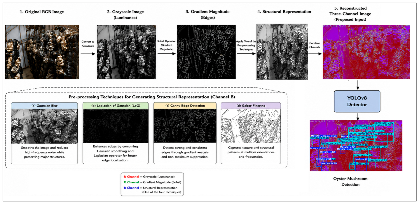
The primary contribution of this study is a new structure-aware RGB channel representation, which aims to improve the robustness of YOLOv8-based oyster mushroom detection in greenhouse conditions. Visual challenges in the cultivation environments of oyster mushrooms include non-uniform illumination, low contrast between the mushrooms and the cultivation substrate, and overlapping mushrooms. In such scenarios, conventional RGB images typically provide limited structural information for accurate object localization, where the detector largely depends on raw color information, which is sensitive to changes in illumination. To address this limitation, the proposed method introduces a novel input representation that explicitly separates the complementary visual information into different image channels before feeding them to the detector. The proposed approach unifies luminance, boundary, and structural information as a three-channel representation, which makes YOLOv8 learn more discriminative geometric features and improves robustness against illumination variation, background clutter, and difficult visual properties of greenhouse cultivation environments. The overall workflow of the proposed method is shown in Figure 1.

First, the original RGB image is converted to a grayscale image, which represents the overall luminance information. The gradient magnitude is then computed from the grayscale image with the Sobel operator to highlight object boundaries and local intensity changes. Finally, one of the four image pre-processing techniques (Gaussian Blur, Laplacian of Gaussian (LoG), Canny edge detection, and Gabor filtering) is used to generate an additional structural representation. These three complementary representations are then combined into a new three-channel image, which is used as the input to the YOLOv8 detector. Specifically, the reconstructed input channels are defined as follows (Equations (1)–(4)).

$$I_{input}=\left.\left[R^{\prime },G^{\prime },B^{\prime }\right.\right]$$

(1)

$$R^{\prime }=I_{gray}$$

(2)

$$G^{\prime }=I_{gradient}$$

(3)

$$B^{\prime }=I_{filter}$$

(4)

Here, $I_{gray}$ denotes the grayscale intensity image; $I_{gradient}$ represents the gradient magnitude obtained from the Sobel operator; and $I_{filter}$ corresponds to one of the filter-based structural representations (Gaussian Blur, Laplacian of Gaussian, Canny edge detection, or Gabor filtering).

Different from standard RGB images, where the three channels encode the red, green, and blue color components, the proposed representation assigns a specific structural role to each channel. The grayscale channel is independent of color but still contains global intensity information. The gradient channel highlights object contours and local shape information, assisting the detector in more accurately capturing the mushroom boundary. The third channel provides additional structural information, which depends on the pre-processing technique used, so that the detector can make use of different image features, such as noise suppression, edge enhancement, or texture representation.

This channel reconstruction is performed offline before model training and inference and does not require modification of the YOLOv8s network architecture. In the revised controlled comparisons, the detector architecture, dataset partition, optimizer configuration, epoch budget, and non-HSV augmentation settings are held constant, while the HSV-augmentation difference in the original RGB baseline is explicitly controlled through an additional RGB (HSV disabled) experiment. Accordingly, only results obtained under matched settings are interpreted as direct input-representation comparisons.

In order to completely evaluate the performance of the proposed representation, four structure-aware channel configurations were investigated, together with two additional ablation controls (described below) that isolate the contribution of each component of the reconstructed input:

• Gray–Gradient–Gaussian (GGGau);
• Gray–Gradient–LoG (GGLoG);
• Gray–Gradient–Canny (GGCanny);
• Gray–Gradient–Gabor (GGGabor);
• Gray–Gray–Gray (GGG), an ablation control isolating the effect of grayscale conversion alone;
• Gray–Gradient–Gray (GGradG), an ablation control isolating the additional effect of the Sobel gradient channel.

The GGG and GGradG configurations were not intended as competing structure-aware representations but as component-wise ablations of the proposed reconstruction, added to isolate the individual contribution of grayscale conversion, the Sobel gradient channel, and the third filter-based channel; their results are reported alongside the main comparison in Section 3.1 and Section 3.2. The traditional RGB input was taken as a baseline and compared with these configurations under the same experimental setup to investigate the effect of different structural representations on feature learning, detection accuracy, and model generalization. In order to make this reproducible, Algorithm 1 shows the full procedure described above for complete channel reconstruction. Given an input RGB image and a filter type to be selected (Gaussian Blur, LoG, Canny or Gabor), the algorithm first computes the grayscale intensity channel and the Sobel gradient magnitude channel, which are common to all four configurations. Then, the respective structural representation is calculated based on the filter type selected and given to the third channel. The three channels are then normalized and fused to generate the final three-channel input image for YOLOv8 training and inference.

Algorithm 1. The algorithm of structure-aware RGB channel reconstruction for oyster mushroom detection

Require: RGB image I; filter type f∈{Gaussian, LoG, Canny, Gabor} Ensure: Reconstructed three-channel image I_input 1. I_gray ← RGB2GRAY(I) 2. G_x ← Sobel_x(I_gray); G_y ← Sobel_y(I_gray) 3. I_gradient ← √(G_x2 + G_y2) 4. I_gradient ← Normalize(I_gradient, 0, 255) 5. if f = Gaussian then 6.  I_filter ← GaussianBlur(I_gray, σ) 7. else if f = LoG then 8.  I_filter ← Laplacian(GaussianBlur(I_gray, σ)) 9. else if f = Canny then 10.  I_filter ← Canny(I_gray, T_low, T_high) 11. else if f = Gabor then 12.  Ifilter ← Σ{θ∈{0°,45°,90°,135°}} |GaborResponse(I_gray, θ)| 13. end if 14. I_filter ← Normalize(I_filter, 0, 255) 15. R′ ← I_gray; G′ ← I_gradient; B′ ← I_filter 16. I_input ← Merge(R′, G′, B′) return I_input

2.3. Image Preprocessing

In this study, five preprocessing operations were explored to study the effect of structural image representations on object detection performance: the traditional RGB image and four grayscale-based preprocessing methods—Gaussian Blur, Laplacian of Gaussian (LoG), Canny edge detection, and Gabor filtering. Combined with the ablation controls and RGB variants described in Section 2.2, these operations give rise to six controlled experimental conditions evaluated in Section 3: RGB (default and HSV-disabled), GGG, GGradG, GGGau, and GGLoG. The Canny- and Gabor-based configurations (GGCanny, GGGabor) were also implemented and initially evaluated, but their results were excluded from the controlled comparison because they originated from an earlier, non-reproducible evaluation run rather than the documented protocol used for the other six conditions (Section 3.2).

2.3.1. Conventional RGB

The baseline setup uses the original RGB images without any preprocessing. Each image is made up of three color channels for the red, green, and blue intensity values as in Equation (5):

$$I_{input}=\left.\left[R,G,B\right.\right]$$

(5)

where (R), (G), and (B) correspond to the red, green, and blue channels. These images were used as direct input to the baseline YOLOv8 model and used as a reference to compare with the proposed structure-aware representations.

2.3.2. Gaussian Blur

Gaussian filtering is a linear smoothing method that removes high-frequency noise while preserving the main structures of an image. It is commonly used as a pre-processing step in computer vision to improve the quality of the image before feature extraction and object detection [3,4]. The Gaussian kernel in two dimensions is given by Equation (6):

$$G\left(x,y\right)={\displaystyle \frac{1}{2\mathsf{\pi }{\sigma }^2}}exp\left(-{\displaystyle \frac{x^2+y^2}{2{\sigma }^2}}\right)$$

(6)

where $\sigma$ denotes the standard deviation controlling the smoothing strength. The filtered image is obtained by

$$I_{Gaussian}=I_{gray}\ast G\left(x,y\right)$$

(7)

where (*) represents the convolution operator. In this study, the standard deviation was set to $\sigma$ = 2.0, which provided sufficient noise suppression while retaining the overall structural outline of the mushroom clusters.

2.3.3. Laplacian of Gaussian (LoG)

The Laplacian of Gaussian (LoG) combines Gaussian smoothing with the Laplacian operator to improve edge localization while reducing sensitivity to image noise. Compared with the conventional Laplacian operator, LoG produces more stable edge responses in noisy images and has been widely adopted in image segmentation and object detection applications [4,15]. The LoG operator is expressed as

$$LoG\left(x,y\right)={\nabla }^2{G}_{\sigma }(x,y)$$

(8)

where the Laplacian operator is defined as Equation (9) and the filtered image is obtained as Equation (10):

$${\nabla }^2={\displaystyle \frac{{\partial }^2}{\partial x^2}}+{\displaystyle \frac{{\partial }^2}{\partial y^2}}$$

(9)

$$I_{LoG}=I_{gray}\ast LoG\left(x,y\right)$$

(10)

The Gaussian smoothing step was applied with $\sigma$ = 1.0, followed by a Laplacian operator with a kernel size of 3 × 3, which was found to provide stable edge responses without excessive noise amplification.

2.3.4. Canny Edge Detection

Canny edge detection is a multi-stage edge-extraction algorithm that aims to achieve accurate localization while minimizing false edge responses [16]. The algorithm is one of the most popular edge detectors in computer vision because of its robustness to different illumination and noise conditions. The Canny algorithm consists of five successive steps:

• Gaussian smoothing for noise suppression.
• Gradient computation using the Sobel operator with a 3 × 3 kernel.
• Non-max suppression.
• Double-threshold edge classification using a low threshold of T_low = 80 and a high threshold of T_high = 160.
• Edge tracking via hysteresis.

The gradient magnitude is computed as in Equation (11), where $G_x$ and $G_y$ denote the horizontal and vertical Sobel gradients, respectively. The resulting normalized gradient-magnitude image was employed as the second channel (G) in the proposed RGB representation.

$$M\left(x,y\right)=\sqrt{G_x^2+G_y^2}$$

(11)

2.3.5. Gabor Filtering

Gabor filtering is an effective texture analysis technique capable of simultaneously representing spatial and frequency information. Because mushroom surfaces exhibit rich texture patterns, Gabor filters provide complementary structural information that may facilitate feature extraction during deep learning [17,18]. The two-dimensional Gabor kernel is defined as Equation (12), where $x^{\prime }$ and $y^{\prime }$ defined as Equations (13) and (14), and $I_{Gabor}$ defined as Equation (15):

$$g\left(x,y\right)=exp\left.\left(-{\displaystyle \frac{x^{\prime 2}+{\gamma }^2{y}^{\prime 2}}{2{\sigma }^2}}\right.\right)cos\left.\left(2\pi {\displaystyle \frac{x^{\prime }}{\lambda }}+\psi \right.\right)$$

(12)

$$x^{\prime }=xcos\theta +ysin\theta$$

(13)

$$y^{\prime }=-xsin\theta +ycos\theta$$

(14)

Here, $\lambda$ is the wavelength, $\theta$ is the orientation angle, $\psi$ denotes the phase offset, $\sigma$ controls the Gaussian envelope, and $\gamma$ represents the spatial aspect ratio.

$$I_{Gabor}=I_{gray}\ast g\left(x,y\right)$$

(15)

A bank of four Gabor filters with orientations θ ∈ {0°, 45°, 90°, 135°} was used, with kernel size 21 × 21, σ = 4.0, λ = 10.0, γ = 0.5, and ψ = 0. The magnitude responses of the four orientations were summed to obtain a single orientation-invariant texture representation, which was then normalized to form the $I_{filter}$ channel.

2.4. YOLOv8 Object Detection Model

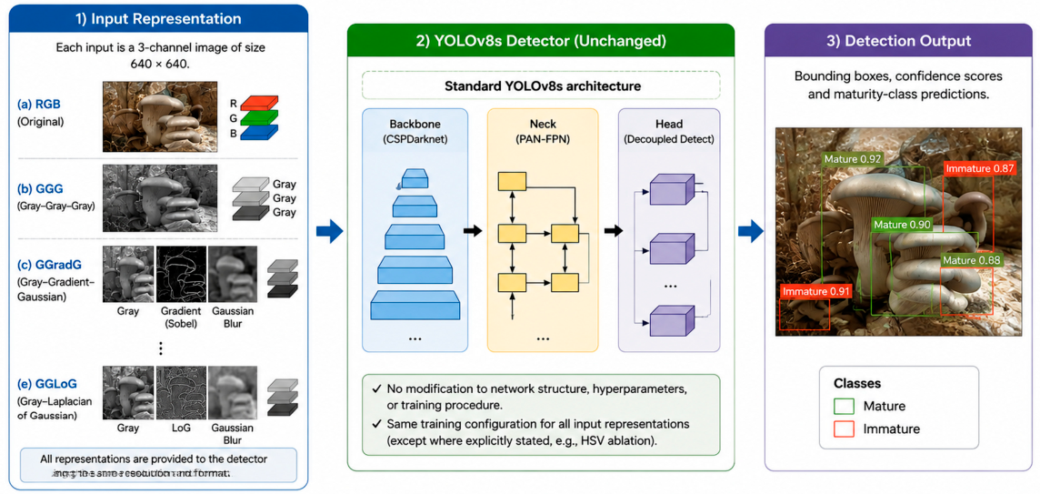
The object detection experiments were carried out using the YOLOv8 object detection framework developed by Ultralytics [19]. YOLOv8 is a single-stage detector that localizes and classifies objects in one forward pass, which offers an effective trade-off between detection accuracy and computational efficiency. YOLOv8 has an anchor-free detection strategy, an improved feature extraction network, and an optimized prediction head as compared to previous versions of YOLO, which leads to better localization accuracy, especially for small and densely distributed objects. A simplified schematic of the overall pipeline, showing the input representations, the unmodified YOLOv8 architecture, and the detection output, is shown in Figure 2.

The backbone is in charge of extracting hierarchical visual features from the input image. YOLOv8 uses a convolutional feature extraction network based on Cross Stage Partial (CSP) concepts with C2f modules that improve gradient flow and reduce computational complexity. During feature extraction, the spatial resolution is progressively reduced, and the semantic representation becomes more discriminative, so that the network can learn low-level texture information and high-level object features [19]. The neck aggregates multi-scale feature maps generated by the backbone. YOLOv8 combines semantic and spatial information at different scales of features by a combination of the Feature Pyramid Network (FPN) and Path Aggregation Network (PAN). This multi-scale feature fusion enhances the detection of objects of different sizes and improves the localization performance of small oyster mushrooms in dense clusters [20,21]. The detection head finally predicts the objects’ locations and class probabilities. Unlike previous versions of YOLO that utilized anchor boxes, YOLOv8 adopts an anchor-free detection method that directly predicts the centers of objects. The design reduces computational complexity, simplifies label assignment, and improves localization accuracy. For every detected mushroom, the detection head simultaneously estimates the bounding-box coordinates, object confidence score, and class probabilities.

In this study, the detector was trained to recognize two classes: immature and mature oyster mushrooms. The YOLOv8s architecture was unchanged across the input-representation experiments. Training controls, including the additional RGB (HSV disabled) experiment introduced to address the augmentation confound, are specified in Section 2.5.

2.5. Experimental Settings

All experiments were performed using the Ultralytics implementation of YOLOv8 (version 8.4.78) in the PyTorch 2.11 deep learning framework [19,22]. Controlled experiments were run with matched architecture, optimizer, epoch budget, image size, and non-HSV augmentation settings; the HSV augmentation difference in the original RGB baseline is explicitly documented and controlled using the additional RGB (HSV disabled) condition described below. The oyster mushroom dataset was divided into training, validation, and test subsets using a 70:15:15 ratio, and the YOLOv8s object detection model was fine-tuned using the proposed dataset of oyster mushrooms as described in Section 2.1. The network was initialized with the pretrained weights of the YOLOv8s network, provided by the Ultralytics framework, and trained on the custom dataset for 200 epochs, with the size of the input image being 640 × 640 pixels. The default batch size of 16 was used for all training. Used automatic optimizer selection from Ultralytics (‘optimizer = auto’), which set the optimizer to AdamW with an initial learning rate of 0.001667, a momentum coefficient of 0.90, and weight decay of 0.0005. To improve computational efficiency, we enabled Automatic Mixed Precision (AMP) training.

The HSV-based color augmentation was turned off by setting the hue, saturation, and value augmentation parameters to 0 for the four structure-aware configurations, since the proposed method reconstructs the RGB channels using the grayscale, gradient magnitude, and filter-based structural representations. For the conventional RGB baseline, we kept the default augmentation settings from Ultralytics, including HSV color jitter, since this setting depends on real color information. Because the four structure-aware configurations and the RGB baseline therefore differed in augmentation strategy as well as input representation, an additional RGB (HSV disabled) control was trained with the same architecture, optimizer, and epoch budget, differing from the RGB baseline only in the HSV augmentation setting; results are reported alongside the main comparison in Section 3.2. The other remaining default augmentation strategies provided by the Ultralytics framework, such as mosaic augmentation, random scaling, translation, horizontal flipping, and random erasing, were retained during training for all configurations. No data augmentation was applied to the validation or test datasets. After training, model selection was based on the highest validation performance, and the final evaluation was performed using the best model on the independent test set; consequently,

Table 2. Validation performance of YOLOv8 at the best checkpoint, for the RGB baseline (default and HSV-disabled), the two component-wise ablation controls (GGG, GGradG), and the structure-aware representations (GGGau, GGLoG), after 200 epochs (all classes).

Structure	Precision	Recall	F1	mAP@0.5	mAP@0.5:0.95	Δ 1 vs. RGB (mAP@0.5)	Convergence
RGB (default HSV)	0.810	0.795	0.802	0.835	0.590	—	Stable
RGB (HSV disabled)	0.793	0.808	0.800	0.833	0.595	−0.002	Stable
GGG (ablation)	0.814	0.792	0.803	0.840	0.589	+0.005	Stable
GGradG (ablation)	0.788	0.805	0.796	0.846	0.597	+0.011	Stable
GGGau	0.801	0.791	0.796	0.838	0.590	+0.003	Stable
GGLoG	0.792	0.802	0.797	0.831	0.586	−0.004	Stable

¹ Δ values denote the difference in mAP@0.5 relative to the conventional RGB baseline.

reports validation-set metrics at the selected checkpoint rather than metrics computed on the training images themselves (see Section 3.1). Training and evaluation were performed on Google Colab on an NVIDIA Tesla T4 GPU (15 GB VRAM). The implementation was written in Python 3.12, PyTorch 2.11, and the Ultralytics YOLOv8 framework. To assess the additional generality of the proposed representation beyond a single architecture, the RGB (HSV disabled), GGG, and GGGau configurations were also trained with RT-DETR-l under an otherwise identical protocol; results are reported in Section 3.4. To assess sensitivity to random initialization, the RGB (HSV disabled), GGG, and GGGau configurations were additionally trained with three random seeds (0, 42, 123); results are reported in Section 3.5.

2.6. Evaluation Metrics

The proposed structure-aware RGB channel representation is intended to enhance the robustness of YOLOv8 by allowing the detector to learn the structural characteristics of oyster mushrooms rather than relying primarily on color information. Therefore, the evaluation protocol was proposed to evaluate the detection accuracy, localization quality, and generalization capability of the detector trained using different input image representations. The detection performance of the standard RGB input and the four structure-aware channel representations proposed in this work (Gaussian Blur, Laplacian of Gaussian, Canny edge detection, and Gabor filtering) was evaluated with the standard object detection metrics provided by the Ultralytics YOLOv8 framework. These metrics give complementary information about accuracy in classification, precision in localization, and overall detection performance.

A bounding box prediction was counted as a true positive (TP) if its Intersection over Union (IoU) with the corresponding ground-truth bounding box was above the defined threshold. False Positives (FP) were predictions that did not overlap sufficiently with a ground-truth object, while False Negatives (FN) were ground-truth objects that were not detected. True negatives (TN) are background areas that were correctly rejected or non-object instances that were correctly identified. Because object detection does not involve a fixed, enumerable set of negative candidates in the way that closed-set classification does, TN-based metrics such as classification accuracy are not well-defined for this task in a way that is comparable across images or datasets; TN is therefore not reported as a standalone count or used in any metric in this study, and only Precision, Recall, F1-score, and mAP are used to evaluate detection performance, consistent with standard object detection practice [23]. The IoU between the predicted and ground-truth bounding boxes is given by Equation (16):

$$IoU={\displaystyle \frac{\mathrm{Intersection}\mathrm{Area}}{\mathrm{Union}\mathrm{Area}}}$$

(16)

Based on TP, FP, and FN, Precision and Recall were calculated as in Equations (17) and (18). Precision quantifies the proportion of correctly detected mushrooms among all predicted detections, whereas Recall measures the proportion of annotated mushrooms successfully detected by the model. To provide a balanced evaluation of both measures, the F1-score was computed as in Equation (19):

$$Precision={\displaystyle \frac{\mathrm{T}\mathrm{P}}{\mathrm{T}\mathrm{P}+\mathrm{F}\mathrm{P}}}$$

(17)

$$Recall={\displaystyle \frac{\mathrm{T}\mathrm{P}}{\mathrm{T}\mathrm{P}+\mathrm{F}\mathrm{N}}}$$

(18)

$$F1-Score=2·{\displaystyle \frac{\mathrm{P}\mathrm{r}\mathrm{e}\mathrm{c}\mathrm{i}\mathrm{s}\mathrm{i}\mathrm{o}\mathrm{n}·\mathrm{R}\mathrm{e}\mathrm{c}\mathrm{a}\mathrm{l}\mathrm{l}}{\mathrm{P}\mathrm{r}\mathrm{e}\mathrm{c}\mathrm{i}\mathrm{s}\mathrm{i}\mathrm{o}\mathrm{n}+\mathrm{R}\mathrm{e}\mathrm{c}\mathrm{a}\mathrm{l}\mathrm{l}}}$$

(19)

The main performance metric was the mean Average Precision (mAP) (Equation (20)), a summary of the area under the Precision–Recall curve.

$$mAP={\displaystyle \frac{1}{N}}{\displaystyle \sum _{i=1}^N}{AP}_i$$

(20)

Two variants of mAP are used: mAP@0.5 is a metric that evaluates detection results with an IoU threshold of 0.50. The mAP@0.5:0.95 metric computes the average of Average Precision over IoU thresholds from 0.50 to 0.95 with a step size of 0.05 [24]. Since mAP@0.5:0.95 requires more accurate localization, it is a stricter evaluation of detector performance and localization accuracy.

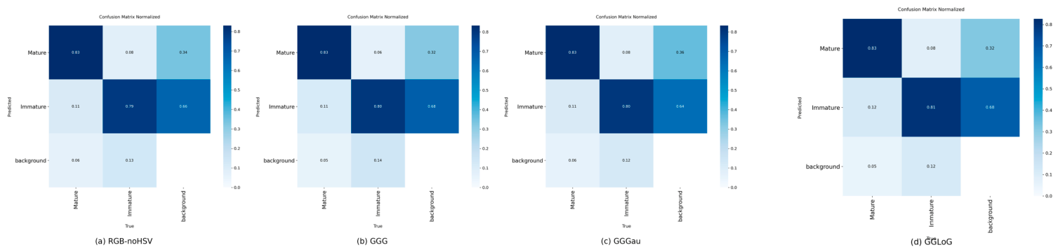
The purpose of the proposed method is to improve feature representation without altering the detection architecture. Therefore, the comparison between the preprocessing methods was conducted using Precision, Recall, F1-score, mAP@0.5, and mAP@0.5:0.95. In addition, normalized confusion matrices were generated for the RGB (HSV disabled), GGG, GGGau, and GGLoG conditions to evaluate class-specific detection performance and to identify common sources of misclassification between immature and mature oyster mushrooms, consistent with the six conditions included in the controlled comparison (Section 3.2). Overall, these metrics give a comprehensive evaluation of the effectiveness of the proposed structure-aware RGB channel representation.

3. Results

This section presents the experimental results obtained using the proposed structure-aware RGB channel representations. First, the training performance for each image representation is analyzed to investigate the detector’s learning behavior. Then, the generalization ability of the trained models is evaluated with the independent test dataset. Finally, the effects of different structural representations on the detection robustness are compared.

3.1. Validation Performance

Table 2 shows the validation-set performance of YOLOv8 at the checkpoint selected for each condition (see Section 2.5), for the conventional RGB input (default and HSV-disabled augmentation), the two component-wise ablation controls (GGG, GGradG), and the proposed structure-aware image representations, after 200 training epochs, evaluated over both mushroom classes combined. All conditions successfully converged the detector and obtained similar validation performance: mAP@0.5 ranged narrowly from 0.831 (GGLoG) to 0.846 (GGradG), a spread of only 0.015, with the RGB baseline (0.835 with default HSV augmentation, 0.833 with HSV disabled) falling within this same narrow band rather than trailing behind the structure-aware representations. Because GGG and GGradG contain no gradient or filter-based structural information at all, and nonetheless match or exceed the full structure-aware configurations on this split, the validation results in Table 2 by themselves do not distinguish between the candidate explanations of grayscale conversion, gradient information, and filter-based structural information; Section 3.2 examines whether the independent test set is more discriminating.

Among the evaluated representations, GGradG obtained the highest validation mAP@0.5 (0.846), narrowly ahead of GGGau (0.838) and the RGB baseline (0.835). The F1-score was likewise similar across conditions, from 0.796 (GGLoG) to 0.803 (GGG). The differences between conditions at validation were small—within about 1.5 percentage points of mAP@0.5—indicating that all configurations, including the two ablation controls that omit gradient and filter information entirely, provided sufficient discriminative information for learning the oyster mushroom classes on this split. Given that three seeds of the RGB, GGG, and GGGau conditions produced a validation mAP@0.5 standard deviation of roughly 0.005–0.01 (Section 3.5), differences of this size should not be interpreted as evidence that any one configuration is reliably superior at validation time; the more informative comparison is generalization to the independent test set, examined next.

Training and validation trajectories were inspected to verify convergence of the evaluated configurations. The principal representations showed broadly stable convergence over the 200-epoch schedule, although the epoch corresponding to the best validation checkpoint differed among configurations. Quantitative comparisons are based on the validation and independent test metrics reported in Table 2 and

Table 3. Independent test-set performance of YOLOv8 for the RGB baseline (default and HSV-disabled), the two component-wise ablation controls (GGG, GGradG), and the structure-aware representations (GGGau, GGLoG), after 200 epochs (all classes), on the fixed random 70:15:15 image-level split.

Structure	Precision	Recall	F1	mAP@0.5	mAP@0.5:0.95	Δ vs. RGB (mAP@0.5)
RGB (default HSV)	0.788	0.760	0.774	0.801	0.562	—
RGB (HSV disabled)	0.760	0.795	0.777	0.803	0.563	+0.002
GGG (ablation)	0.753	0.806	0.779	0.813	0.564	+0.012
GGradG (ablation)	0.756	0.765	0.760	0.787	0.548	−0.014
GGGau	0.762	0.776	0.769	0.787	0.552	−0.014
GGLoG	0.768	0.782	0.775	0.788	0.556	−0.013

. Training performance was comparable, but training accuracy does not necessarily imply greater detector robustness. Therefore, the models were further tested on an independent test set to assess their generalization capability.

3.2. Test Performance

The results on unseen images are given in Table 3. On this random image-level split, the differences between conditions at test time were considerably smaller than an earlier internal evaluation had suggested, and a preliminary result reporting a large RGB test-time drop (mAP@0.5 of 0.590) could not be reproduced when the evaluation was repeated end-to-end under the protocol described in Section 2.5; the reproduced RGB result is reported here instead (see Section 3.1 note and the accompanying repository log). The standard RGB representation (default HSV augmentation) achieved a test mAP@0.5 of 0.801 and a mAP@0.5:0.95 of 0.562, essentially unchanged from its validation performance (0.835 and 0.590, respectively) once the validation-vs-test comparison is made on a like-for-like basis. Disabling HSV augmentation for RGB did not meaningfully change this picture (test mAP@0.5 = 0.803). Critically, the GGG ablation control—grayscale conversion only, with no gradient or filter channel—achieved the highest test mAP@0.5 of all six conditions in Table 3 (0.813), while GGradG, GGGau, and GGLoG all scored slightly lower on the test set (0.787, 0.787, and 0.788, respectively) than either RGB condition or GGG. This pattern indicates that, on the random split, none of the six conditions shows a generalization advantage over the others that is clearly larger than the run-to-run variation quantified in Section 3.5, and provides no support for the hypothesis that the Sobel gradient channel or the third filter-based channel (Gaussian, LoG) improves test-set generalization beyond what grayscale conversion alone achieves.

The Gaussian Blur (GGGau) and LoG (GGLoG) representations maintained a small validation-to-test gap, consistent with earlier expectations: GGGau moved from a validation mAP@0.5 of 0.838 to a test mAP@0.5 of 0.787 (a difference of 0.051), and GGLoG moved from 0.831 to 0.788 (a difference of 0.043). However, the RGB baseline showed a comparably small gap in the reproduced evaluation (0.835 to 0.801, a difference of 0.034), and the GGG ablation control showed the smallest gap of all six conditions (0.840 to 0.813, a difference of 0.027). Because the ablation control generalizes at least as well as the full structure-aware representations, these results do not support the interpretation that the Sobel gradient channel or the third filter-based channel specifically promotes more robust geometric feature learning; the more parsimonious reading is that grayscale conversion (common to GGG, GGradG, GGGau, and GGLoG alike) is associated with the small, consistent validation-to-test gap observed across all four of these conditions, while the RGB baseline’s gap in this reproduced run is of a similar order of magnitude rather than dramatically larger. Figure 3 shows the YOLOv8 detections of the RGB image (a) and the reconstructed image (b) with LoG.

The GGCanny and GGGabor configurations were also implemented and initially evaluated, but in an earlier run that predated the discovery that the RGB baseline result could not be reproduced end-to-end (see above). Because their available results were therefore not obtained under the same documented, reproducible protocol as the other six conditions in this study, we do not include their numerical results in the controlled comparison reported in this manuscript (Table 2, Table 3,

Table 4. Per-class test performance of YOLOv8 for each image representation after 200 epochs.

Structure	Precision	Recall	F1	mAP@0.5	mAP@0.5:0.95
RGB (default HSV)—Mature	0.783	0.763	0.773	0.803	0.594
RGB (default HSV)—Immature	0.793	0.757	0.775	0.799	0.530
RGB (HSV disabled)—Mature	0.745	0.803	0.773	0.794	0.591
RGB (HSV disabled)—Immature	0.774	0.786	0.780	0.813	0.536
GGG (ablation)—Mature	0.745	0.834	0.787	0.823	0.601
GGG (ablation)—Immature	0.762	0.778	0.770	0.803	0.527
GGradG (ablation)—Mature	0.755	0.753	0.754	0.790	0.578
GGradG (ablation)—Immature	0.756	0.776	0.766	0.784	0.519
GGGau—Mature	0.750	0.797	0.773	0.787	0.575
GGGau—Immature	0.774	0.755	0.764	0.788	0.529
GGLoG—Mature	0.762	0.813	0.787	0.794	0.590
GGLoG—Immature	0.774	0.750	0.762	0.782	0.522

and

Table 5. Test performance under a chronological (date-wise) holdout compared to the random 70:15:15 image-level split, for the four principal representations selected for chronological evaluation: RGB (HSV disabled), GGG, GGGau, and GGLoG.

Structure	Precision	Recall	F1	mAP@0.5	mAP@0.5:0.95	Δ vs. Random Split
RGB (HSV disabled)—random split	0.760	0.795	0.777	0.803	0.563	—
RGB (HSV disabled)—chronological split	0.444	0.441	0.443	0.311	0.153	−0.492
GGG—random split	0.753	0.806	0.779	0.813	0.564	—
GGG—chronological split	0.365	0.489	0.418	0.251	0.126	−0.562
GGGau—random split	0.762	0.776	0.769	0.787	0.552	—
GGGau—chronological split	0.409	0.431	0.420	0.285	0.141	−0.502
GGLoG—random split	0.768	0.782	0.775	0.788	0.556	—
GGLoG—chronological split	0.385	0.450	0.415	0.279	0.139	−0.509

); re-evaluating them under the corrected protocol is identified as a direction for future work (Section 4).

The per-class breakdown of test results for the mature and immature mushroom classes is shown in Table 4. The pattern is consistent with the combined-class results in Table 3: F1-scores for the six conditions (RGB default/HSV-disabled, GGG, GGradG, GGGau, GGLoG) fall within a narrow band of roughly 0.75–0.79 for both classes, with no condition showing a clearly superior precision–recall trade-off once accounting for run-to-run variation (Section 3.5).

In summary, on the random image-level split, the differences between the RGB baseline, the two ablation controls (GGG, GGradG), and the structure-aware representations (GGGau, GGLoG) were modest and, based on the repeated-seed results in Section 3.5, not clearly distinguishable from run-to-run noise for several pairwise comparisons. The clearest generalization failure identified so far is not RGB versus structure-aware representations, but rather performance under the random split versus performance under the chronological holdout (Section 3.3), where every condition tested showed a large drop. The GGCanny and GGGabor conditions were excluded from Table 2, Table 3 and Table 4 for the reasons given above; re-evaluating them under the corrected protocol remains a direction for future work (Section 4).

Taken together, these results temper the original hypothesis of this work: rather than concluding that focusing on geometric and boundary information (via gradient or filter-based channels specifically) allows the detector to learn more transferable representations than classical RGB, the evidence to date is more consistent with grayscale conversion being the primary factor associated with the small, consistent validation-to-test gap observed for the color-independent conditions, while the RGB baseline’s gap, once correctly measured, is of a similar order of magnitude on this split. This interpretation is broadly consistent with evidence from the wider computer vision literature that CNN-based models can rely heavily on texture and color statistics rather than object shape, and that reducing this reliance can improve robustness [25], though we emphasize that our ablation does not directly measure texture or shape reliance and cannot confirm this mechanism on its own. We view this as a more modest but more reliable finding than originally reported, and one that motivates the additional ablation, cross-architecture, and temporal-holdout work reported in Section 3.3, Section 3.4 and Section 3.5.

Figure 4 reports normalized confusion matrices for RGB (HSV disabled), GGG, GGGau, and GGLoG on the independent test set. These four conditions compare the controlled RGB baseline, the grayscale-only ablation, and the two structure-aware inputs the earlier review specifically requested. All four show similar class-level error patterns, consistent with the modest differences in aggregate test metrics. Mature instances are correctly assigned at approximately 83% in every condition, while Immature instances are correctly assigned at approximately 79–81% at the evaluated operating point, and background is confused with Immature (64–68%) more often than with Mature (32–36%) across all four. The background row and column represent unmatched detections and unmatched ground-truth objects rather than conventional true negatives.

3.3. Chronological (Date-Wise) Holdout

To assess sensitivity to the temporal/scene correlation discussed in Section 2.1, RGB (HSV disabled) and the GGG ablation control were additionally trained and evaluated on a chronological split, in which the earliest 70% of images (by acquisition date) were used for training, the next 15% for validation, and the most recent 15% for testing, with no random shuffling. Table 5 compares test-set performance under this chronological split to the corresponding random-split result reported in Table 3.

Both conditions show a large drop in test-set mAP@0.5 under the chronological holdout—approximately 0.49 for RGB (HSV disabled) and 0.56 for GGG—far larger than any difference observed between representations on the random split (Section 3.2). This confirms that the random image-level split allows temporally or scene-correlated information to be shared between training and test images, and that performance under the random split substantially overstates generalization to genuinely unseen acquisition periods for both the baseline and the ablation control. GGGau and GGLoG show the same pattern: both drop from a random-split mAP@0.5 in the high 0.78–0.79 range to a chronological mAP@0.5 near 0.28 (Table 5), with F1 collapsing to 0.420 and 0.415 respectively — a decline of similar magnitude to that seen for RGB (HSV disabled) and GGG. This confirms, across all four principal representations evaluated, that the large chronological-holdout gap is not specific to the baseline or the ablation control, and that no structure-aware representation evaluated in this study is more temporally robust than RGB.

3.4. Cross-Architecture Check: RT-DETR

To assess whether the pattern observed for YOLOv8 extends to a different detector architecture, the RGB (HSV disabled), GGG, and GGGau conditions were additionally trained with RT-DETR-l [26], a real-time end-to-end transformer-based detector, under an otherwise identical protocol (200 epochs, same random 70:15:15 split, same image size). Initial training with the default batch size of 16 showed unstable convergence under some conditions; a batch size of 8 was used for the results reported here, which trained stably for all three conditions.

Table 6. Test performance of RT-DETR-l for the RGB (HSV disabled) baseline and two structure-aware conditions, on the same random 70:15:15 split used in Table 2, Table 3 and Table 4.

Structure	Precision	Recall	F1	mAP@0.5	mAP@0.5:0.95	Δ vs. RGB (mAP@0.5)
RGB (HSV disabled)	0.768	0.808	0.787	0.809	0.565	—
GGG (ablation)	0.713	0.754	0.733	0.748	0.528	−0.061
GGGau	0.716	0.789	0.751	0.764	0.534	−0.045

reports test-set performance.

Under RT-DETR, the RGB baseline outperformed both GGG and GGGau, the opposite ordering from the corresponding YOLOv8 comparison in Table 3. This indicates that the generalization pattern observed for YOLOv8 in this study does not transfer to RT-DETR on this dataset, and that the proposed channel reconstruction should not be assumed to be architecture-independent without further, architecture-specific validation. This is consistent with reports elsewhere in agricultural object detection that RT-DETR and YOLO-family detectors can respond differently to the same input and training conditions, with trade-offs between accuracy and inference cost that do not always favor the same architecture [27]. We report this negative result because it directly bears on the architecture-independence claim made elsewhere in this manuscript, and because a training-stability issue (requiring a smaller batch size than the YOLOv8 experiments) was itself a relevant, reportable methodological finding.

3.5. Sensitivity to Random Initialization

To quantify run-to-run variability, consistent with reporting practices recommended for machine learning experiments more generally [28,29], the RGB (HSV disabled), GGG, and GGGau conditions were each retrained from three random seeds (0, 42, 123) under an otherwise identical protocol. The underlying training/validation/test partition (Section 2) was held fixed across all three seeds; only the model-training random seed was varied.

Validation-set mAP@0.5 and mAP@0.5:0.95 for each seed, together with the mean and standard deviation across seeds, are reported in

Table 7. Validation performance across three random seeds for three conditions, with mean ± standard deviation.

Structure	Seed 0	Seed 42	Seed 123	Mean ± SD	Metric
RGB (HSV disabled)	0.833	0.850	0.842	0.842 ± 0.009	Val. mAP@0.5
RGB (HSV disabled)	0.592	0.594	0.587	0.591 ± 0.004	Val. mAP@0.5:0.95
GGG (ablation)	0.840	0.837	0.854	0.844 ± 0.009	Val. mAP@0.5
GGG (ablation)	0.589	0.590	0.597	0.592 ± 0.004	Val. mAP@0.5:0.95
GGGau	0.846	0.847	0.844	0.846 ± 0.002	Val. mAP@0.5
GGGau	0.600	0.593	0.597	0.597 ± 0.004	Val. mAP@0.5:0.95

. The corresponding test-set evaluation across the same three seeds is reported in

Table 8. Independent test-set performance across the same three random seeds (0, 42, 123) for three conditions, with mean ± standard deviation.

Structure	Precision	Recall	F1	mAP@0.5	mAP@0.5:0.95
RGB (HSV disabled)	0.771 ± 0.008	0.789 ± 0.004	0.780 ± 0.004	0.795 ± 0.008	0.553 ± 0.007
GGG (ablation)	0.758 ± 0.020	0.792 ± 0.021	0.774 ± 0.002	0.800 ± 0.004	0.559 ± 0.004
GGGau	0.758 ± 0.010	0.778 ± 0.012	0.768 ± 0.002	0.796 ± 0.008	0.553 ± 0.011

.

Seed-to-seed standard deviation in validation mAP@0.5 is approximately 0.002–0.009 for the three conditions tested, and approximately 0.004 for mAP@0.5:0.95. This is comparable to, or larger than, several of the “Δ vs. RGB” differences reported to three decimal places in Table 2 (e.g., +0.003 for GGGau, −0.004 for GGLoG), indicating that such small differences are not distinguishable from run-to-run noise in this setup and should not be interpreted as evidence that one configuration reliably outperforms another. We report point estimates from a single seed elsewhere in Table 2, Table 3 and Table 4 and Table 6 for the conditions not included in this seed study, and flag this as a limitation (Section 4) rather than treat single-run differences below approximately 0.01 mAP@0.5 as established findings.

As on the validation set, seed-to-seed standard deviation on the test set (approximately 0.004–0.011 for mAP@0.5:0.95, and 0.004–0.008 for mAP@0.5) is comparable to or larger than the differences between configurations: GGG shows a marginally higher mean mAP@0.5 and mAP@0.5:0.95 than RGB (HSV disabled), but within run-to-run noise, and GGGau shows no consistent advantage over either. This reinforces the conclusion drawn from the validation-set seed study—that grayscale replication performs comparably to RGB, and the added structural channel does not yield a stable improvement—while extending it to test-set performance, which is the metric the paper’s claims ultimately rest on.

4. Discussion

The study explored the potential for the construction of the RGB input channels from the structural image representation to improve the robustness of YOLOv8 in the detection of oyster mushrooms. The proposed approach differs from conventional object detection pipelines that directly use RGB images by substituting the original color channels with grayscale intensity, gradient magnitude, and complementary structural information prior to feeding the images to the detector. Experimental results show that this simple pre-processing strategy has a strong impact on the learning behavior and generalization capability of the detector.

One of the most notable results is that, on the random image-level split, the RGB baseline, GGG, GGradG, GGGau, and GGLoG all showed a broadly similar, modest gap between validation and test performance (Section 3.2), rather than the large RGB-specific gap suggested by a preliminary evaluation that could not be reproduced. The component-wise ablation is the most informative comparison here: GGG, which contains only grayscale intensity replicated across all three channels with no gradient or filter information at all, generalized at least as well as GGradG, GGGau, and GGLoG on this dataset. This pattern is more consistent with grayscale conversion (i.e., removing reliance on raw hue and saturation) being the operative factor than with the Sobel gradient channel or the third filter-based channel (Gaussian, LoG) contributing an additional, independently measurable benefit.

We had initially hypothesized that the Gaussian and LoG channels would specifically promote geometric or boundary-based feature learning beyond what grayscale conversion alone provides; the ablation results do not support this stronger version of the hypothesis, at least as measured by aggregate detection metrics on this dataset and split. We report this as a genuine, if less dramatic, finding rather than adjust the hypothesis post hoc: color-independent grayscale conversion appears to be doing most of the work, and the additional structural channels examined here neither help nor hurt performance appreciably within the noise level established by the repeated-seed experiments in Section 3.5. Confirming or ruling out a smaller, gradient- or filter-specific contribution would require evidence beyond aggregate mAP, such as feature visualization, targeted corruption or ablation studies isolating illumination versus texture sensitivity, or evaluation on a dataset where color is more strongly confounded with the target class than in the present one. The GGCanny and GGGabor conditions are not included in this comparison, consistent with their exclusion from the principal controlled analysis (Section 3.2).

These results temper, rather than confirm, the original hypothesis that gradient- or filter-based structural information specifically drives the detector’s robustness: the ablation in Table 2, Table 3 and Table 4 indicates that grayscale conversion is the more likely operative factor, at least on this dataset and random split. What the results do support is a narrower but still useful claim: that input representation—specifically, whether the detector relies on raw color or on a color-independent representation—is a factor worth considering in agricultural object detection, alongside the more commonly studied architecture and training-strategy improvements [9,10]. Most previous studies on agricultural object detection directly use RGB images as network inputs and focus on architectural or training-strategy improvements; the current work suggests that the choice of input representation deserves comparable attention, while cautioning, based on the chronological-holdout and cross-architecture results in Section 3.3 and Section 3.4, against assuming that a gain observed on a random, single-architecture split will transfer to genuinely unseen time periods or to other detector architectures.

The proposed approach also has a practical advantage in its simplicity. The preprocessing operations rely on classical, non-learned filters (grayscale conversion, a Sobel gradient, and a Gaussian, LoG, Canny, or Gabor transform) that are computed once, offline, before training and inference, and require no modification to the YOLOv8 architecture, loss function, or optimization procedure, so the method can be integrated into an existing YOLO-based pipeline without retraining the detector’s architecture. We have not yet measured the added preprocessing latency, memory footprint, or throughput on embedded or edge hardware, so we do not claim a demonstrated efficiency advantage for deployment; quantifying these costs (e.g., per-image preprocessing time on representative embedded platforms) is identified as necessary future work in Section “Limitations” below before any deployment-oriented claim can be made.

Several limitations should be noted, some of which are addressed in part by the additional experiments reported in Section 3.3, Section 3.4 and Section 3.5, and some of which remain open. First, the random image-level split used for Table 2, Table 3 and Table 4 does not control for temporal correlation between images collected with a fixed camera; the chronological holdout in Section 3.3 shows a substantial drop in test-set performance for every condition evaluated under it, indicating that the random-split numbers in Table 2, Table 3 and Table 4 likely overstate performance under a genuine temporal or facility-level distribution shift, and this holdout has not yet been completed for the two remaining controlled conditions (RGB default HSV, GGradG). Second, the component-wise ablation in Table 2, Table 3 and Table 4 (GGG, GGradG) indicates that grayscale conversion, rather than the gradient or filter-based channels specifically, accounts for most of the measured effect on this dataset; whether the gradient and filter channels provide benefit under other conditions (e.g., the chronological split, other datasets, or corruption/robustness tests) has not been established and would require further evidence, such as feature visualization or controlled corruption tests, beyond aggregate mAP. Third, the GGCanny and GGGabor configurations were excluded from the controlled comparison in this manuscript because their available results originated from an earlier, non-reproducible evaluation run rather than the documented protocol used for the other six conditions; re-evaluating them under the corrected protocol remains a direction for future work. Fourth, the experiments were performed on a single dataset collected at one cultivation facility with a fixed camera; further validation on datasets collected under different cameras, facilities, illumination conditions, and mushroom varieties would better demonstrate robustness. Fifth, four filter-based preprocessing techniques were implemented in this study, but only two (Gaussian Blur, LoG) are included in the controlled comparison for the reasons given in Section 3.2; future work could re-evaluate the Canny- and Gabor-based configurations under the corrected protocol, and test additional structural representations, including wavelet transforms, adaptive edge enhancement, morphological filtering, or learnable pre-processing networks. Sixth, we evaluated one alternative architecture, RT-DETR, in addition to YOLOv8 (Section 3.4); on this dataset, RT-DETR did not show the same generalization pattern as YOLOv8, with the RGB baseline outperforming the structure-aware and ablation conditions, so the benefit observed for YOLOv8 should not be assumed to transfer to other detector architectures. Finally, we have not measured preprocessing latency, memory footprint, or throughput on embedded or edge hardware, so no efficiency claim is made for deployment scenarios pending such measurements.

We therefore offer color-independent channel reconstruction as a simple, input-level preprocessing strategy worth further investigation on YOLOv8-family detectors, while withholding the stronger claims of demonstrated computational efficiency, architecture independence, and geometric-feature-learning mechanism made in earlier drafts of this work, pending the additional evidence identified in Section 4 (Limitations) as necessary future work; the RT-DETR comparison in Section 3.4 indicates this strategy’s benefit should not be assumed to generalize across detector architectures.