Configurational Dynamics of Agricultural Carbon Reduction in China’s Yellow River Basin

Abstract

Agricultural carbon reduction (ACR) is important for the green transformation of agriculture and ecological protection in the Yellow River Basin. However, ACR is not driven by a single factor. How different conditions combine and change over time remains unclear. Based on the technology–organization–environment (TOE) framework, this study examines 77 cities in the Yellow River Basin from 2017 to 2022. Six antecedent conditions are considered: agricultural technological innovation (ATI), agricultural mechanization (AM), government environmental attention (GEA), government fiscal intervention (GFI), agricultural industrial structure (AIS), and urbanization (URB). Multi-period fuzzy-set qualitative comparative analysis (fsQCA) is used to identify the pathways to high ACR, their temporal evolution, and regional differences. The results show that (1) no single antecedent condition is necessary for high ACR in either period; (2) four high-ACR pathways are identified in the baseline period (2017–2019), comprising three types: agricultural structure–urbanization synergy, agricultural technological innovation-led, and technology–equipment–urbanization synergy; (3) four high-ACR pathways are also identified in the transition period (2020–2022). AIS is present in all four pathways, compared with only two pathways in the baseline period, and combines with AM or URB in different configurations; and (4) regional comparisons reveal alternative configurations of production and governance conditions. Upstream pathways include technology–equipment–government combinations, midstream pathways retain both technological and structural alternatives, and downstream pathways show a more pervasive role for AIS in the later period. These findings suggest that effective ACR policies should match local production and governance conditions rather than uniformly increase individual policy inputs.

1. Introduction

Agriculture and food systems are major sources of global greenhouse gas emissions. Promoting low-carbon agricultural transformation has therefore become important for climate change mitigation, food security, and sustainable agricultural development [1,2]. Agricultural emissions come from multiple sources and processes. They are shaped not only by production inputs and farming practices but also by technological progress, production structure, and resource use [3]. Studies on China have identified substantial regional differences in agricultural emissions and have distinguished declining emission intensity from changes in total emissions [4,5]. China’s No. 1 Central Document for 2026 further calls for the wider use of green production and water-saving irrigation technologies and the development of ecological and low-carbon agriculture [6]. This shows that green and low-carbon transformation remains an important policy direction for Chinese agriculture. The Yellow River Basin is a major agricultural production region in China. It is also ecologically fragile and faces strong resource and environmental constraints [7]. Understanding the multiple pathways to agricultural carbon reduction (ACR) and their spatial and temporal differences is therefore important for designing region-specific mitigation strategies.

Existing studies on ACR can be broadly divided into two groups. The first focuses on the measurement, efficiency, and spatiotemporal evolution of agricultural carbon emissions. At the farm level, Virkkunen et al. [8] developed a land-use greenhouse gas accounting framework for different farm and crop types in Finland and found clear differences in emission intensity across production systems. Huan et al. [4] found substantial regional variation in China’s agricultural carbon emissions, with different grain-producing regions showing distinct convergence patterns and carbon-peaking trends. Gong et al. [9] evaluated agricultural carbon-reduction performance from the perspective of carbon emission efficiency and found that provincial agricultural carbon emission efficiency generally improved from 2015 to 2021, except for a temporary decline during 2016–2017, with marked regional heterogeneity and declines in several provinces during 2020–2021. In the Yellow River Basin, Nie et al. [10] incorporated both agricultural carbon emissions and carbon sinks into an agricultural carbon-effect assessment and examined its spatiotemporal relationship with food security. The second group examines the drivers of agricultural carbon emissions. For instance, Li et al. [11] found that agricultural trade liberalization reduces carbon emission intensity through technology spillovers and industrial structure optimization, with stronger effects in coastal regions and areas with low environmental regulation. Wang et al. [12] demonstrated that agricultural mechanization significantly reduces greenhouse gas intensity through the reallocation of land, labor, and agrochemical inputs, with harvesting operations exerting the strongest effect. Zhang et al. [13] showed that agricultural subsidy adjustments reduce carbon emissions by optimizing cropping structures and promoting green innovation and machinery services, with more pronounced effects in eastern regions and major grain-producing areas. Urbanization reduces agricultural carbon emissions through structural adjustment, production efficiency improvement, and technological advancement, with positive spatial spillover effects on neighboring regions [14]. In addition, carbon trading pilots have been found to curb agricultural carbon emissions through technological innovation, with the reduction effect moderated by regional resource allocation efficiency and accompanied by positive spillovers to neighboring pilot regions [15].

Existing studies provide an important basis for understanding the spatial patterns and drivers of agricultural carbon emissions. However, several gaps remain. First, most studies focus on the net effects of individual factors. Less attention has been paid to the complementarity, substitution, and synergy among different conditions. It therefore remains unclear how different combinations of conditions can produce high ACR. Second, the dynamic evolution of ACR pathways has received limited attention. As green agricultural transformation progresses, technological capacity, governance capacity, and regional development conditions may change over time. The configurations formed by these conditions may also change across periods [16,17]. It is therefore necessary to examine the temporal stability and evolution of both core conditions and configurational pathways. Third, existing studies have examined agricultural emissions and green production at national, provincial, and county levels. However, configurational differences within the Yellow River Basin remain underexplored. In particular, systematic comparisons of ACR pathways across the upstream, midstream, and downstream regions are still limited.

To address these gaps, this study examines 77 cities in the Yellow River Basin from 2017 to 2022. Based on the technology–organization–environment (TOE) framework, six antecedent conditions are considered: agricultural technological innovation (ATI), agricultural mechanization (AM), government environmental attention (GEA), government fiscal intervention (GFI), agricultural industrial structure (AIS), and urbanization (URB). Multi-period fuzzy-set qualitative comparative analysis (fsQCA) is used to identify the configurations associated with high ACR and their evolution across periods. Regional differences across the upstream, midstream, and downstream areas are also compared. This study makes three contributions. First, it applies the TOE framework from a configurational perspective and examines the synergy, substitution, and complementarity among technological, organizational, and environmental conditions. This extends research beyond the net effects of individual factors. Second, it extends the application of dynamic configurational analysis to prefecture-level cities in the Yellow River Basin and examines the continuity, adjustment, and reconfiguration of the roles of conditions and ACR pathways across periods. Third, it compares configurational pathways across the three major regions of the Yellow River Basin. This provides more detailed evidence for differentiated agricultural carbon-reduction strategies.

2. Theoretical Framework

2.1. TOE Framework

The technology–organization–environment (TOE) framework was proposed by Tornatzky and Fleischer [18]. It argues that technological innovation and its implementation are shaped not only by technology itself but also by organizational characteristics and the external environment [18]. Its main value lies in explaining complex behavior and performance from multiple dimensions and integrating factors at different levels [19,20]. The TOE framework was originally developed for research on organizational technology adoption. In recent years, it has also been applied to environmental governance and sustainable development. For example, Tan et al. [21] combined TOE and fsQCA to identify multiple pathways to high municipal waste-sorting performance in China, demonstrating that technological, organizational, and environmental conditions jointly shape waste-sorting outcomes. Similarly, Wang et al. [22] applied the TOE framework and fsQCA to investigate carbon emission reduction among Chinese firms, showing that different configurations of TOE factors can generate multiple low-carbon pathways. In the agricultural sector, Qi et al. [23] further demonstrated that combinations of digital technology, organizational conditions, and external environments lead to multiple pathways toward higher agricultural eco-efficiency, with spatial heterogeneity across regions. These studies collectively demonstrate that environmental and sustainability outcomes emerge from the interaction of multiple contextual conditions rather than from any single factor alone [21,22,23]. Combining TOE with configurational analysis allows technological, organizational, and environmental conditions to be examined as interdependent configurations rather than as factors with fixed net effects. This makes the framework suitable for a configurational analysis of ACR.

Configurational theory emphasizes causal complexity. The role of the same condition may differ across configurations, and different combinations of conditions may lead to the same outcome. This reflects conjunctural causation and equifinality [24]. Recent configurational research further suggests that complex outcomes should not be explained by searching for a single universally dominant factor. Greater attention should instead be paid to complementarity, substitution, and overall fit among conditions [25]. Related empirical evidence supports this contextual view. Qayyum et al. [26] found that the effects of technology adoption on agricultural emissions vary significantly across country groups, suggesting that the same technological condition can produce different outcomes depending on the broader contextual environment. Shi et al. [27] found that the association between agricultural green technological innovation and agricultural carbon productivity differs across innovation actors. This evidence concerns the green subset of agricultural innovation rather than all ATI. Related city-level research also identified economic-development thresholds in the relationship between general technological innovation and carbon emission intensity [28], providing broader evidence of contextual heterogeneity rather than direct evidence on agricultural emissions. These findings suggest that ACR also results from the joint effects of multiple conditions. It cannot be explained by technological innovation, government action, or economic development alone. Rather, it depends on how different conditions work together.

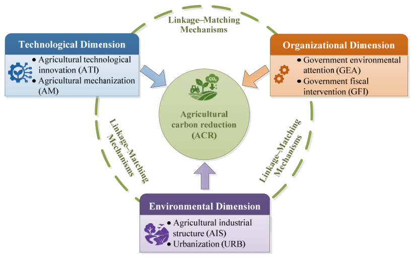
Accordingly, this study adapts the TOE framework to the context of urban ACR. The technological dimension captures the innovation and production equipment needed for green agricultural production and includes ATI and AM. The organizational dimension treats local governments as key actors in low-carbon agricultural governance. It reflects their attention to environmental issues and their capacity to mobilize fiscal resources, represented by GEA and GFI. The environmental dimension reflects the structural context of agricultural production and urban–rural development, represented by AIS and URB. This results in an analytical framework with three dimensions and six antecedent conditions, as shown in Figure 1.

2.2. Technological Dimension

The technological dimension captures agricultural innovation and production equipment that may affect resource use and emission intensity. This study considers two aspects: technological innovation and production equipment.

ATI refers to the development and diffusion of technologies used in agricultural production, including crop breeding, production inputs, field management, plant protection, agricultural machinery, and smart agriculture [29,30,31]. These technologies may affect land productivity, resource-use efficiency, production organization, and factor allocation, although their environmental effects depend on the type of technology and its adoption context [29,30,31]. Related research suggests that technological progress and diffusion can contribute to lower agricultural carbon emission intensity [3]. However, the emission-reduction effect of ATI does not materialize automatically in every context. Wu et al. [31] found that input-oriented innovation has limited or even negative effects on grain yield, whereas field-management innovation produces more consistent yield gains. Although this evidence concerns productivity rather than carbon emissions, it shows that the effects of ATI vary by innovation type. Furthermore, the potential emission-reduction effect of ATI depends on the extent of technology adoption and diffusion, as well as on complementary organizational and institutional conditions [26,32]. Accordingly, a higher level of ATI does not necessarily translate into high ACR; its effectiveness depends on its alignment with agricultural mechanization, production structure, government action, and other conditions.

AM refers to the extent to which agricultural production relies on machinery across key field operations, including tillage, sowing, fertilization, irrigation, and harvesting, reflecting the modernization of agricultural equipment and production practices [12,33]. Mechanization can improve the precision and efficiency of these operations, reduce resource inputs per unit of output, and facilitate land consolidation and labor reallocation. Wang et al. [12] found that AM can significantly reduce greenhouse gas emission intensity through the reallocation of land, labor, and agricultural chemical inputs. However, the carbon-reduction effect of AM also depends on equipment efficiency, production scale, and other production conditions. A higher level of AM therefore does not necessarily produce high ACR in every context. Based on these considerations, ATI and AM are selected as the two conditions in the technological dimension.

2.3. Organizational Dimension

In the context of urban ACR, the organizational dimension reflects the attention and resource-mobilization capacity of local governments in promoting green and low-carbon agricultural transformation. Local governments can influence agricultural producers through policy agendas and environmental governance objectives. They can also provide fiscal support for green technology adoption, agricultural infrastructure, and public services. This study therefore uses GEA and GFI to represent the organizational dimension.

GEA reflects the priority that local governments assign to environmental and low-carbon issues when allocating their limited attention [21]. Greater attention can help place these issues on the policy agenda and strengthen environmental governance through policy design, regulation, and resource allocation. Previous research shows that GEA can affect pollutant and greenhouse gas emissions, although its effects vary across regions [34]. Government attention therefore does not directly translate into emission-reduction performance. Its effect also depends on whether governance resources, technologies, and industrial conditions work together effectively.

In this study, GFI reflects the relative scale of general public budget expenditure in the local economy rather than expenditure earmarked specifically for agriculture or environmental protection [35]. Fiscal mobilization can provide resources for agricultural infrastructure, socialized services, technology adoption, and public governance. Evidence from agricultural subsidy adjustments, although based on a narrower fiscal instrument than GFI, identifies production restructuring, green innovation, and mechanization services as relevant transmission channels [13]. Related city-level evidence shows that the carbon-reduction effects of fiscal institutions depend on economic development and environmental regulation [36]. Higher GFI therefore does not necessarily lead directly to higher ACR; its role depends on resource allocation and its interaction with technological and production conditions. Based on these considerations, GEA and GFI are selected as the two conditions in the organizational dimension.

2.4. Environmental Dimension

The environmental dimension reflects the structural context of agricultural production and urban–rural development. Compared with technological conditions and local government actions, AIS and URB mainly represent the broader setting in which agricultural production takes place. They also influence the allocation of technology, capital, labor, and other production factors. This study therefore uses AIS and URB to represent the environmental dimension.

AIS reflects the share of agricultural output in the total output of agriculture, forestry, animal husbandry, and fisheries, thereby capturing the structural characteristics of regional agricultural production [11,37]. Different subsectors vary in energy use, chemical input intensity, and biological emission characteristics; for instance, crop farming relies heavily on nitrogen fertilizer and irrigation energy, while livestock production involves distinct biological emission processes. Optimizing this structure, such as shifting toward lower-carbon and water-efficient cropping patterns, can reduce agricultural carbon emission intensity and improve resource allocation [37]. Li et al. [11] further show that changes in agricultural production structure are an important mechanism affecting agricultural carbon emissions and may interact with technological progress. AIS may therefore influence not only the composition of agricultural emissions but also the conditions under which ATI and AM take effect.

URB refers to the process of population concentration in urban areas and the associated transformation of urban–rural development patterns, which provides the broader context for agricultural production [14,38]. Urbanization is accompanied by rural labor migration, changes in land management, the development of agricultural services, and improvements in infrastructure; these changes can affect agricultural inputs and resource allocation efficiency [38,39]. Lei et al. [14] found that urbanization can promote low-carbon agricultural transformation through structural adjustment, technological progress, and improved production efficiency, with clear spatial spillover effects. However, cities differ in their stage of urbanization, agricultural production base, and resource endowments. The way URB interacts with other conditions may therefore vary across regions. Based on these considerations, AIS and URB are selected as the two conditions in the environmental dimension.

3. Research Methods

3.1. Multi-Period fsQCA

Qualitative comparative analysis (QCA) is based on set theory and Boolean algebra. It is suitable for examining complex causal relationships in which multiple antecedent conditions jointly produce an outcome. It can identify conjunctural causation, equifinality, and causal asymmetry [24]. Regression-based approaches generally estimate the net association between individual variables and an outcome, whereas QCA examines set-theoretic relationships of necessity and sufficiency involving combinations of conditions [24,40]. The two approaches therefore address different research questions. A statistically significant coefficient in regression indicates an association with the outcome under a specified model, but does not determine whether a variable is a necessary or sufficient condition for achieving a high level of the outcome [24]. In practice, a variable that appears insignificant in isolation may still play a critical role depending on the presence or absence of other conditions. For example, in the context of ACR, it cannot be assumed that a linear increase in a single factor will independently drive emission reduction [11,13]. QCA complements net-effect analysis by examining how combinations of conditions jointly produce outcomes. This configurational perspective is useful for policy design because it identifies which combinations of conditions can jointly support high performance. Moreover, depending on the data type, QCA methods can be classified into mvQCA (multi-value QCA, suitable for multi-valued data), csQCA (crisp-set QCA, suitable for binary data), and fsQCA (fuzzy-set QCA, suitable for continuous data) [24]. Since the six antecedent conditions and the outcome variable in this study are continuous, this study adopts fsQCA, which converts raw values into membership scores between 0 and 1 through calibration, thereby preserving differences in degree across cases. The fsQCA 4.1 software developed by Charles C. Ragin and Sean Davey was used for calibration and configurational analysis.

The mechanisms underlying ACR may change with shifts in the policy environment, technological conditions, and agricultural production structure. A single-period or pooled static analysis may not fully capture these changes [16,35]. Multi-period QCA compares configurations across different periods and examines how configurational relationships evolve over time [41,42]. Specifically, multi-period QCA conducts calibration, necessity analysis, and sufficiency analysis separately for each period, and then compares core conditions, peripheral conditions, and configuration structures across periods [41]. Multi-period QCA allows us to assess whether the identified configurations are specific to a particular period or persist across different time windows, thereby providing evidence on the temporal stability of these configurations [41,43]. Previous studies have shown that a condition may act as a core driver in one period but become peripheral or even redundant in another; accordingly, a configuration that is effective in one period may no longer apply in another, or may be replaced by alternative configurations [35,39,44]. Therefore, this study applies multi-period fsQCA and treats each city-year observation as a case. Calibration, necessity analysis, and sufficiency analysis are conducted separately for each period. The core conditions, peripheral conditions, configuration types, and covered cases are then compared across periods. These cross-period comparisons allow us to identify the continuity, adjustment, and reconfiguration of ACR pathways.

3.2. Variable Measurement

Outcome variable. For the empirical analysis, high ACR is operationalized as relatively low AGS CO₂ emission intensity within each period. High ACR therefore represents the relative low-carbon performance of the sampled cities rather than a direct measure of a sustained decline in emissions, an increase in agricultural productivity, or a comprehensive reduction in all agricultural greenhouse gases. Following the emission-intensity approach [45], AGS CO₂ emission intensity is calculated as total CO₂ emissions reported under EDGAR’s Agricultural Soils (AGS) sector divided by constant-price gross agricultural output. The outcome is reverse-calibrated so that lower emission intensity corresponds to higher membership in the high-ACR set. City-level AGS CO₂ emissions are derived from the EDGAR GHG 2024 database, with a spatial resolution of 0.1° × 0.1°. The gridded emission data are overlaid with prefecture-level administrative boundaries. For grid cells intersecting more than one city, emissions are allocated in proportion to the area of overlap and then summed within each city. Nominal gross agricultural output is deflated using the provincial agricultural producer price index (previous year = 100) and expressed in constant 2017 prices. Annual AGS CO₂ emissions are expressed in tonnes, while gross agricultural output is measured in CNY 10,000. The resulting intensity is therefore expressed as tonnes of CO₂ per CNY 10,000 of constant-price gross agricultural output. The emission boundary is limited to CO₂ reported under EDGAR’s AGS sector and does not include CH₄, N₂O, or emissions reported under other EDGAR sectors.

Antecedent conditions. ATI is measured by the number of granted invention patents in the International Patent Classification (IPC) A01 category per 10,000 people, reflecting the level of local agricultural technological innovation [30,46]. AM is measured by total agricultural machinery power per capita and reflects the level of agricultural mechanization [47]. GEA is measured by the frequency of environmental keywords, such as “environmental protection”, “pollution”, “emission reduction”, and “low carbon”, per 1000 words in local government work reports. This measure reflects the attention of local governments to environmental and low-carbon issues [34]. GFI is measured by the ratio of general public budget expenditure to regional GDP and reflects the extent of local government involvement in economic and social development and fiscal resource allocation [48]. AIS is measured by the share of agricultural output in the total output of agriculture, forestry, animal husbandry, and fisheries and reflects the internal structure of agricultural production [49]. URB is measured by the share of the urban population in the total population and reflects the level of population urbanization [50].

3.3. Sample Selection and Data Sources

On 18 September 2019, ecological protection and high-quality development in the Yellow River Basin was elevated to a major national strategy. Because the announcement occurred near the end of 2019 and policy implementation may involve a time lag, this study compares two equal three-year windows within the balanced panel initially compiled for 77 cities over 2017–2022. Period 1 (2017–2019) covers the pre-strategy years and the announcement year, whereas Period 2 (2020–2022) represents the early transition stage following the announcement. Equal-length windows reduce differences in case frequency caused solely by unequal observation periods and support a focused comparison of configurational evolution within this six-year period. The analysis therefore does not assess developments after 2022.

Considering the spatial scope of the Yellow River Basin, the completeness of prefecture-level administrative units, and data availability, 77 prefecture-level and higher-level cities are included. The study covers 2017–2022 and contains 462 city–year observations. Each period includes 231 city–year cases. For n antecedent conditions, there are theoretically 2ⁿ logical combinations [24]. In this study, the six antecedent conditions can form 64 logical combinations, and the sample size in each period sufficiently meets the requirements for the number of cases in QCA. To examine regional heterogeneity, the sample cities are further divided into upstream, midstream, and downstream regions following Tan et al. [39]. Regional configurational analyses are then conducted.

AGS CO₂ emission data are obtained from the EDGAR GHG 2024 database, while prefecture-level administrative boundary data are obtained from the Tianditu platform of the National Geomatics Center of China (Map Approval Number: GS (2024) 0650). ATI data are obtained from the China National Intellectual Property Administration. GEA data are compiled from local government work reports. Data on general public budget expenditure, regional GDP, total agricultural machinery power, agricultural output, total output of agriculture, forestry, animal husbandry, and fisheries, and urban population are mainly collected from the China City Statistical Yearbook, provincial and municipal statistical yearbooks, and statistical bulletins on national economic and social development.

3.4. Calibration

fsQCA requires the conversion of raw data into set-membership scores ranging from 0 to 1. No external theoretical thresholds are currently available to define uniformly high and low levels of the variables across cities in the Yellow River Basin. In addition, this study focuses on relative configurational differences among cities within each period. Following previous multi-period QCA research [35], the direct calibration method is therefore used, and the calibration anchors are determined from the sample distribution within each period.

For ATI, AM, GEA, GFI, AIS, and URB, the 75th, 50th, and 25th percentiles within each period are set as the thresholds for full membership, the crossover point, and full non-membership, respectively. Because lower agricultural carbon emission intensity indicates higher ACR, the outcome is calibrated in the opposite direction. The 25th, 50th, and 75th percentiles of agricultural carbon emission intensity are set as the thresholds for full membership, the crossover point, and full non-membership, respectively. After direct calibration, antecedent-condition membership scores exactly equal to 0.50 were recoded as 0.501 before truth-table analysis. No corresponding adjustment was made to the outcome membership scores. The calibration anchors are reported in

Table 1. Calibration of the Conditions and Outcome.

Period	Condition/Outcome	Full Non-Membership	Crossover	Full Membership	Mean	SD
Period 1	ACR	0.040	0.024	0.018	0.033	0.023
	ATI	0.014	0.027	0.066	0.051	0.062
	AM	0.532	0.791	1.107	0.905	0.538
	GEA	6.876	8.527	10.339	8.862	2.800
	GFI	0.138	0.181	0.269	0.232	0.140
	AIS	0.501	0.601	0.663	0.584	0.130
	URB	49.029	54.880	64.350	57.140	13.037
Period 2	ACR	0.040	0.024	0.017	0.032	0.022
	ATI	0.006	0.023	0.054	0.042	0.056
	AM	0.602	0.899	1.253	1.016	0.641
	GEA	7.203	9.052	10.582	9.277	2.988
	GFI	0.143	0.170	0.248	0.218	0.122
	AIS	0.504	0.600	0.662	0.584	0.133
	URB	51.695	59.010	68.020	60.866	13.135

.

4. Results and Analysis

4.1. Necessity Analysis

Table 2. Necessity Analysis of Individual Conditions.

Antecedent Condition	Period 1				Period 2
	High ACR		Non-High ACR		High ACR		Non-High ACR
	Consistency	Coverage	Consistency	Coverage	Consistency	Coverage	Consistency	Coverage
ATI	0.625	0.656	0.449	0.451	0.559	0.594	0.508	0.513
~ATI	0.477	0.474	0.657	0.627	0.541	0.536	0.598	0.564
AM	0.662	0.658	0.455	0.434	0.630	0.647	0.478	0.467
~AM	0.431	0.452	0.642	0.645	0.482	0.492	0.640	0.622
GEA	0.530	0.549	0.543	0.539	0.498	0.510	0.575	0.561
~GEA	0.555	0.559	0.546	0.527	0.571	0.585	0.498	0.486
GFI	0.441	0.459	0.654	0.652	0.460	0.477	0.626	0.618
~GFI	0.665	0.667	0.457	0.439	0.631	0.640	0.470	0.453
AIS	0.625	0.637	0.489	0.477	0.688	0.684	0.433	0.409
~AIS	0.487	0.498	0.629	0.617	0.406	0.429	0.666	0.670
URB	0.579	0.599	0.512	0.507	0.540	0.568	0.524	0.525
~URB	0.523	0.528	0.595	0.575	0.548	0.548	0.569	0.541

Note: “~” denotes the absence of a condition.

reports the necessity analysis for high and non-high ACR. No antecedent condition or its negation reaches the consistency threshold of 0.90 in either period. The necessity consistency of AIS for high ACR is 0.625 in Period 1 and 0.688 in Period 2, both below this threshold. Thus, none of the individual conditions examined is necessary for either outcome under the adopted calibration. Sufficiency analysis is subsequently used to examine combinations of conditions associated with high and non-high ACR.

4.2. Sufficiency Analysis

Following previous QCA studies, the raw consistency threshold and PRI consistency threshold are set at 0.80 and 0.70, respectively [21]. Each period contains three years of panel data. To avoid configurations supported only by repeated observations from the same city, the case-frequency threshold is set at 4. Core and peripheral conditions are identified by comparing the intermediate and parsimonious solutions. Conditions appearing in both solutions are treated as core conditions, whereas those appearing only in the intermediate solution are treated as peripheral conditions [40]. The configurational results for the two periods are reported in

Table 3. Configurational Results for ACR in Period 1.

Condition	High ACR				Non-High ACR
	H1a	H1b	H2	H3	NH1	NH2	NH3	NH4
ATI	▲	◯	⬤	⬤	◯	◯	△	⬤
AM	△	△	▲	⬤	◯	◯		◯
GEA	◯	▲	▲	◯		◯	⬤	⬤
GFI	◯	◯	◯	◯	▲		⬤	⬤
AIS	⬤	⬤		◯		△	◯	◯
URB	⬤	⬤	◯	⬤	◯	▲	◯	⬤
Raw coverage	0.094	0.071	0.128	0.164	0.285	0.123	0.125	0.073
Unique coverage	0.043	0.040	0.072	0.103	0.184	0.071	0.043	0.045
Consistency	0.831	0.937	0.930	0.834	0.886	0.921	0.898	0.952
Solution coverage	0.337				0.447
Solution consistency	0.847				0.883

Note: ⬤ indicates core presence; ◯ indicates core absence; ▲ indicates peripheral presence; △ indicates peripheral absence. The same notation is used below.

and

Table 4. Configurational Results for ACR in Period 2.

Condition	High ACR				Non-High ACR
	S1	S2	S3	S4	NS1a	NS1b
ATI		△	◯		◯	◯
AM	⬤	⬤	△	△	◯	◯
GEA	◯	◯		△	▲	△
GFI	⬤		◯	△	▲	△
AIS	⬤	⬤	⬤	▲	◯	◯
URB	△	△	▲	▲		▲
Raw coverage	0.163	0.165	0.125	0.156	0.125	0.088
Unique coverage	0.033	0.030	0.046	0.068	0.096	0.058
Consistency	0.826	0.875	0.921	0.883	0.893	0.884
Solution coverage	0.357				0.183
Solution consistency	0.866				0.881

.

4.2.1. Configurational Results for Period 1

Table 3 shows four pathways to high ACR in Period 1. The solution coverage is 0.337 and the solution consistency is 0.847. Four pathways lead to non-high ACR, with a solution coverage of 0.447 and a solution consistency of 0.883. High and non-high ACR arise from different combinations of conditions. The presence of multiple pathways and distinct configurations for the two outcomes further reflects equifinality and causal asymmetry. Covered cases are reported below in the form of “city_year”.

(1) High ACR

Agricultural structure–urbanization synergy pathway (H1a and H1b). Both H1a and H1b identify AIS and URB as core conditions, while the configurations differ in other conditions. In H1a, ATI is present as a peripheral condition, while AM is peripherally absent and GEA and GFI are absent as core conditions. In H1b, GEA is present as a peripheral condition, while ATI and GFI are absent as core conditions and AM is peripherally absent. AIS can change the composition of agricultural emission sources. URB can support low-carbon agricultural transformation through factor mobility, structural adjustment, and higher production efficiency [11,14]. Thus, H1a and H1b show that when AIS and URB provide strong support, high ACR can be achieved either through ATI or through government environmental attention, and does not necessarily require simultaneous improvements in AM and GFI. H1a has a raw coverage of 0.094 and a consistency of 0.831, while H1b has a raw coverage of 0.071 and a consistency of 0.937. Cases covered by H1a include Xi’an_2018, Jinan_2018–2019, Luoyang_2019, and Zaozhuang_2018–2019. Cases covered by H1b include Jiayuguan_2017–2019 and Jiaozuo_2017–2018. Jinan, for example, has a high level of urbanization and a favorable basis for agricultural restructuring. These conditions support ACR through urban–rural factor flows and production restructuring.

Agricultural technological innovation-led pathway (H2). In H2, ATI is present as a core condition, with AM and GEA present as peripheral conditions, while GFI and URB are absent as core conditions. AIS is unspecified in this configuration. H2 has a raw coverage of 0.128 and a consistency of 0.930, showing that high ACR can be associated with this technological and organizational combination without requiring high GFI or URB. Typical cases include Anyang_2017–2018, Xinxiang_2017–2018, Luohe_2017–2018, and Nanyang_2017.

Technology–equipment–urbanization synergy pathway (H3). H3 combines ATI, AM and URB as core conditions, with GEA, GFI and AIS absent as core conditions. This pathway has a raw coverage of 0.164, the highest among the four pathways, and a consistency of 0.834. This suggests that the combination of technological innovation, production equipment, and urbanization can be associated with high ACR even when GEA, GFI, and the share of agricultural output are low. Previous research shows that AM can reduce greenhouse gas emission intensity by reallocating land, labor, and agricultural chemical inputs [12]. However, its effect on agricultural carbon efficiency can be nonlinear and region-specific [51]. The effect of AM therefore depends on its alignment with technological innovation, urbanization, and other production conditions. Typical cases include Weihai_2017, Yantai_2017–2019, Weifang_2017–2019, Jining_2017 and 2019, Tai’an_2017, Rizhao_2018, and Qingdao_2019.

Overall, Period 1 shows clear condition substitution. ATI can combine with AIS and URB (H1a), with AM and GEA (H2), or with AM and URB (H3). When ATI is weak, GEA can substitute for it within the AIS–URB framework (H1b). Notably, GFI is absent in all four high-ACR pathways, indicating that high fiscal intervention is not a necessary condition for high ACR in the baseline period. Thus, the baseline period does not show one stable model of ACR. Instead, several technology–production–development combinations coexist.

(2) Non-High ACR

NH1 and NH2 show the core absence of ATI, while NH3 shows the peripheral absence of ATI. NH1 and NH2 further show the core absence of AM. NH1 is characterized by the peripheral presence of GFI and the core absence of URB. NH2 is characterized by the peripheral presence of URB, the core absence of GEA, and the peripheral absence of AIS. NH3 is characterized by the presence of both GEA and GFI and the absence of AIS and URB. NH4 shows the presence of ATI, GEA, GFI, and URB, but the core absence of AM and AIS. These configurations indicate that non-high ACR is associated with different combinations involving low ATI, low AM, or a low share of agricultural output. The presence of GEA or GFI in some pathways does not compensate for these configurational conditions. Non-high ACR is therefore not simply the reverse of high ACR.

4.2.2. Configurational Results for Period 2

Table 4 identifies four pathways to high ACR in Period 2. The solution coverage is 0.357 and the solution consistency is 0.866. Two pathways lead to non-high ACR, with a solution coverage of 0.183 and a solution consistency of 0.881. Compared with Period 1, one clear change is the role of AIS. It is present as a core condition in three of the four high-ACR configurations (S1, S2, and S3) and as a peripheral condition in S4, while it is absent as a core condition in both non-high-ACR configurations. This indicates a stronger role for AIS in the transition period.

(1) High ACR

Mechanization–fiscal input–agricultural structure pathway (S1). In S1, AM, GFI, and AIS are present as core conditions, while GEA is absent as a core condition and URB is peripherally absent. This pathway has a raw coverage of 0.163 and a consistency of 0.826. This shows that the combination of AM, GFI, and AIS can support ACR even when GEA is weak and URB provides limited support. Cases covered by S1 include Weinan_2020, Xinyang_2020, Zhoukou_2020, Liaocheng_2020–2021, Shangqiu_2020, Nanyang_2020, Kaifeng_2020 and 2022, and Anyang_2022.

Mechanization–agricultural structure pathway (S2). In S2, AM and AIS are present as core conditions, while GEA is absent as a core condition and ATI is peripherally absent. This pathway has a raw coverage of 0.165, the highest among the four pathways, and a consistency of 0.875. This shows that the core combination of AM and AIS is associated with high ACR even when ATI and GEA are low. Cases covered by S2 include Shangqiu_2020–2022, Nanyang_2021, Weinan_2020, Zhoukou_2020, Kaifeng_2022, Heze_2022, and Anyang_2022.

Agricultural structure–urbanization pathway (S3). In S3, AIS is present as a core condition, ATI and GFI are absent as core conditions, AM is peripherally absent, and URB is present as a peripheral condition. This pathway has a raw coverage of 0.125 and a consistency of 0.921. This shows that AIS can support ACR together with URB, even when ATI, GFI, and AM are weak. Typical cases include Jiayuguan_2021–2022, Zibo_2022, Xi’an_2022, Jiaozuo_2022, Luoyang_2022, Zaozhuang_2022, and Baoji_2022.

Agricultural structure–urbanization pathway with limited supporting conditions (S4). In S4, AIS and URB are present as peripheral conditions, while AM, GEA, and GFI are peripherally absent. This pathway has a raw coverage of 0.156 and a consistency of 0.883. This configuration shows that the peripheral presence of AIS and URB is associated with high ACR when AM, GEA, and GFI are low. Typical cases include Xi’an_2020–2021, Jiayuguan_2022, Luoyang_2020–2022, Zibo_2020, Jinan_2020–2021, and Zaozhuang_2020 and 2022.

(2) Non-High ACR

NS1a and NS1b share the same core structure: ATI, AM, and AIS are absent. In NS1a, GEA and GFI are present as peripheral conditions. In NS1b, GEA and GFI are peripherally absent, while URB is present as a peripheral condition. The peripheral presence of GFI in NS1a and its peripheral absence in NS1b should not be interpreted as either a positive or negative independent effect of fiscal intervention. Rather, the presence of GFI does not compensate for the joint core absence of ATI, AM, and AIS in NS1a. Previous research indicates that agricultural subsidies can influence carbon emissions through production restructuring, green innovation, and mechanization services [13]. Thus, the configurational role of fiscal intervention depends on how fiscal resources are matched with technological, equipment, and production-structure conditions.

4.2.3. Evolution of Configurational Pathways

Although four high-ACR pathways are identified in each period, the roles and combinations of antecedent conditions change over time.

First, AIS becomes more important as a core condition. In Period 1, AIS is present as a core condition only in H1a and H1b. In Period 2, AIS is present as a core condition in S1, S2, and S3, and as a peripheral condition in S4. At the same time, it is absent as a core condition in both non-high-ACR configurations, NS1a and NS1b. AIS becomes a condition shared by all identified high-ACR pathways in Period 2, although its core or peripheral status varies across configurations. This suggests that, in the transition period, high ACR becomes more consistently associated with a production structure that is combined with machinery use, urbanization, or fiscal resources.

Second, ATI is no longer present as a core condition in the identified high-ACR pathways in Period 2, whereas AM retains this role in S1 and S2. In Period 1, ATI is present as a core condition in H2 and H3, and as a peripheral condition in H1a. ATI appears either alongside AIS and URB or alongside AM in technology-led pathways. AM also acts as a core condition in H3. In Period 2, ATI is peripherally absent in S2 and absent as a core condition in S3, while it is unspecified in S1 and S4. By contrast, AM remains a core condition in S1 and S2. These changes concern the configurational roles of ATI and AM and do not establish changes in their independent effects on ACR. Instead, the configurational relevance of ATI and AM depends more strongly on production structure and other supporting conditions. Yang et al. [51] also find nonlinear and spatially heterogeneous effects of AM on agricultural carbon emission efficiency. These findings are consistent with the contextual dependence of agricultural equipment.

Third, organizational conditions play different roles across configurations, with neither GEA nor GFI consistently present in all high-ACR pathways. In Period 2, GFI is present as a core condition in S1, absent as a core condition in S3, and peripherally absent in S4, while it is unspecified in S2. In the non-high-ACR configurations, GFI is present as a peripheral condition in NS1a and peripherally absent in NS1b. The mixed configurational roles of GFI should not be interpreted as evidence of a negative effect. Instead, fiscal input alone cannot guarantee better carbon-reduction performance. Its effect depends on whether fiscal resources are effectively linked to technology diffusion, equipment improvement, and agricultural restructuring. City-level studies also show that the carbon-reduction effects of fiscal institutions and resource allocation depend on economic development, environmental regulation, and industrial conditions [36]. The match between fiscal resources and the agricultural production base may therefore matter more than the scale of fiscal intervention alone.

Overall, the number of high-ACR pathways remains unchanged, but their composition shifts. Period 1 includes both pathways involving AIS and pathways without its presence. In Period 2, AIS is present in all four pathways, combining with AM in S1 and S2 and with URB in S3 and S4. The main temporal change is therefore the more widespread presence of AIS and the changing roles of technological and organizational conditions. This pattern of a more widely shared structural condition with changing supporting conditions is also consistent with the dynamic adaptation emphasized in multi-period configurational analysis [39,41].

4.3. Robustness Tests

Robustness is assessed through changes in solution fit and configurational composition under alternative analytical choices [52]. Specifically, the tests adjust the truth-table thresholds, change the calibration percentiles, and replace the period-specific calibration anchors used in the baseline analysis with common anchors derived from the pooled sample. The results are reported in

Table A1. Robustness Check (Increased Raw Consistency Threshold).

Condition	Period 1								Period 2
	High ACR		Non-High ACR						High ACR			Non-High ACR
	R1	R2	NR1	NR2	NR3	NR4	NR5	NR6	R3	R4	R5	NR7	NR8
ATI	◯	⬤	△	△	◯	◯	△	⬤	◯	◯		◯	◯
AM	△	▲	◯	△	◯	◯		◯	▲	△	△	◯	◯
GEA	▲	▲	⬤		◯	◯	⬤	⬤	◯		◯	▲	△
GFI	◯	◯	▲	▲	▲		⬤	⬤	◯	◯	◯	▲	△
AIS	⬤			△	◯	◯	◯	◯	⬤	⬤	⬤	◯	◯
URB	⬤	◯	◯	△		▲	◯	⬤	△	▲	▲		▲
Raw coverage	0.071	0.128	0.162	0.148	0.138	0.123	0.125	0.073	0.118	0.125	0.156	0.125	0.088
Unique coverage	0.043	0.101	0.081	0.002	0.003	0.047	0.043	0.045	0.075	0.046	0.078	0.096	0.058
Consistency	0.937	0.930	0.904	0.982	0.977	0.921	0.898	0.952	0.977	0.921	0.883	0.893	0.884
Solution coverage	0.171		0.394						0.277			0.183
Solution consistency	0.930		0.908						0.927			0.881

Note: ⬤ indicates core presence; ◯ indicates core absence; ▲ indicates peripheral presence; △ indicates peripheral absence. The same notation is used below.

,

Table A2. Robustness Check (Increased PRI Consistency Threshold).

Condition	Period 1							Period 2
	High ACR		Non-High ACR					High ACR			Non-High ACR
	R1	R2	NR1	NR2	NR3	NR4	NR5	R3	R4	R5	NR6	NR7
ATI	◯	⬤	◯	△	◯	△	⬤	◯	◯		◯	◯
AM	△	▲	◯	△	◯	◯	◯	⬤	△	△	◯	◯
GEA	▲	▲	◯		◯	⬤	⬤	◯		◯	▲	△
GFI	◯	◯	▲	▲		▲	⬤		◯	◯	▲	△
AIS	⬤		◯	△	◯		◯	▲	⬤	⬤	◯	◯
URB	⬤	◯		△	▲	◯	⬤	△	▲	▲		▲
Raw coverage	0.071	0.128	0.138	0.148	0.123	0.162	0.073	0.165	0.125	0.156	0.125	0.088
Unique coverage	0.043	0.101	0.003	0.002	0.047	0.081	0.045	0.121	0.046	0.078	0.096	0.058
Consistency	0.937	0.930	0.977	0.982	0.921	0.904	0.952	0.875	0.921	0.883	0.893	0.884
Solution coverage	0.171		0.350					0.324			0.183
Solution consistency	0.930		0.925					0.884			0.881

,

Table A3. Robustness Check (Increased Case Frequency Threshold).

Condition	Period 1							Period 2
	High ACR			Non-High ACR				High ACR			Non-High ACR
	R1	R2	R3	NR1	NR2	NR3	NR4	R4	R5	R6	NR5
ATI	▲	◯	⬤	◯	△	◯	▲		◯	⬤	◯
AM	△	◯	⬤	◯	△	◯	◯	⬤	◯	△	◯
GEA	◯	⬤	◯	◯		◯	⬤	◯	▲	◯	▲
GFI	◯	◯	◯	▲	▲	△	⬤	⬤	◯	△	⬤
AIS	⬤	⬤	◯		▲	△	△	⬤	⬤	⬤	◯
URB	⬤	⬤	⬤	△	△	▲	▲	◯	⬤	▲	◯
Raw coverage	0.094	0.071	0.164	0.184	0.200	0.090	0.073	0.163	0.091	0.118	0.092
Unique coverage	0.047	0.048	0.123	0.048	0.071	0.051	0.046	0.126	0.057	0.072	0.092
Consistency	0.831	0.937	0.834	0.875	0.845	0.895	0.952	0.826	0.954	0.905	0.944
Solution coverage	0.265			0.360				0.305			0.092
Solution consistency	0.833			0.883				0.867			0.944

,

Table A4. Robustness Check (Alternative Calibration Anchors).

Condition	Period 1							Period 2
	High ACR				Non-High ACR			High ACR				Non-High ACR
	R1	R2	R3	R4	NR1	NR2	NR3	R5	R6	R7	R8	NR4	NR5
ATI	▲		⬤	⬤	◯	◯	⬤		△	◯		◯	◯
AM	△	△	▲	⬤	◯	◯	◯	⬤	⬤	△	△	◯	◯
GEA		▲	▲	◯		◯	⬤	◯	◯		△	▲	△
GFI	◯	◯	◯	◯	▲		⬤	⬤		◯	△	▲	△
AIS	⬤	⬤		◯		△	◯	⬤	⬤	⬤	▲	◯	◯
URB	▲	▲	◯	⬤	◯	▲	⬤	△	△	▲	▲		▲
Raw coverage	0.177	0.157	0.159	0.188	0.316	0.150	0.096	0.192	0.198	0.145	0.184	0.149	0.120
Unique coverage	0.034	0.036	0.067	0.094	0.227	0.069	0.045	0.029	0.028	0.038	0.065	0.096	0.066
Consistency	0.843	0.855	0.938	0.868	0.880	0.900	0.937	0.841	0.876	0.913	0.888	0.896	0.877
Solution coverage	0.404				0.434			0.383				0.215
Solution consistency	0.852				0.881			0.868				0.876

and

Table A5. Robustness Check (Pooled Calibration Anchors).

Condition	Period 1								Period 2
	High ACR					Non-High ACR			High ACR				Non-High ACR
	R1	R2	R3	R4	R5	NR1	NR2	NR3	R6	R7	R8	R9	NR4	NR5
ATI	▲		▲	⬤	△	◯	◯	⬤		△	◯		△	◯
AM	△	△	▲	⬤	△	◯	◯	◯	⬤	⬤	△	△	◯	△
GEA		▲	▲	◯	△		◯	⬤	◯	◯		△	▲	◯
GFI	◯	◯	◯	◯	◯	⬤	△	⬤	⬤		◯	△	⬤	△
AIS	⬤	⬤		◯	⬤		◯	◯	⬤	⬤	⬤	▲	◯	◯
URB	⬤	⬤	◯		◯	◯	▲	⬤	△	△	▲	▲		▲
Raw coverage	0.154	0.123	0.136	0.194	0.076	0.309	0.082	0.073	0.149	0.160	0.140	0.153	0.127	0.093
Unique coverage	0.039	0.027	0.065	0.113	0.030	0.264	0.045	0.046	0.026	0.032	0.058	0.061	0.094	0.061
Consistency	0.823	0.851	0.912	0.837	0.843	0.877	0.879	0.941	0.807	0.853	0.912	0.888	0.907	0.862
Solution coverage	0.433					0.402			0.351				0.188
Solution consistency	0.826					0.878			0.862				0.881

.

First, following previous research [21], the raw consistency threshold is increased from 0.80 to 0.85, the PRI threshold from 0.70 to 0.75, and the case frequency threshold from four to five. Raising either the raw consistency threshold or the PRI threshold reduces the number of Period 1 high-ACR pathways from four to two, with solution coverage falling from 0.337 to 0.171 in both tests. Raising the frequency threshold retains three pathways, with coverage of 0.265. In Period 2, each adjustment retains three high-ACR pathways, with coverage of 0.277, 0.324, and 0.305, respectively. AIS remains present in all these Period 2 pathways, although it is not always a core condition. These results preserve the broad presence of AIS in the transition period but also show that pathway composition and empirical coverage are sensitive to threshold selection.

Second, following previous research [53], the calibration anchors are changed from the 75th, 50th, and 25th percentiles to the 80th, 50th, and 20th percentiles. As in the baseline analysis, anchors are calculated separately for the two periods, and the outcome is reverse-calibrated. This test yields four high-ACR pathways in each period. Period 2 solution coverage increases from 0.357 to 0.383, while consistency changes from 0.866 to 0.868. AIS remains present in all four Period 2 pathways, as a core condition in three and a peripheral condition in one. Thus, its more widespread presence is retained without implying an identical core status across all pathways.

Third, all 462 city–year observations are pooled to calculate common calibration anchors at the 75th, 50th, and 25th percentiles. The common anchors are then applied to both periods, after which the configurational analyses are conducted separately for each period. Under this specification, the number of Period 1 high-ACR pathways increases from four to five, whereas Period 2 retains four pathways. For Period 2, solution coverage is 0.351 and consistency is 0.862, compared with 0.357 and 0.866 in the baseline analysis. AIS remains present in all four Period 2 pathways, as a core condition in three and a peripheral condition in one. In the non-high-ACR solutions, ATI, AM, and AIS remain absent, although their core or peripheral status changes in some specifications.

In summary, the robustness tests show that the main findings remain stable across alternative thresholds and calibration strategies. In particular, AIS remains widely present in the Period 2 high-ACR configurations, and the distinction between high- and non-high-ACR configurations is maintained. Although the number and coverage of individual pathways vary across specifications, these changes do not alter the main conclusions regarding temporal configurational differences.

4.4. Further Analysis

Previous studies show clear regional differences in agricultural carbon emissions and carbon-reduction processes in China [4,54]. The combinations of conditions driving green development also differ across the Yellow River Basin [39]. To further examine regional differences in ACR and their evolution, multi-period fsQCA is conducted separately for the upstream, midstream, and downstream regions. The upstream region includes 20 cities (60 city-year observations per period), the midstream region includes 27 cities (81 city-year observations per period), and the downstream region includes 30 cities (90 city-year observations per period). The raw consistency threshold remains 0.80 and the PRI consistency threshold remains 0.70. Because the regional samples are smaller, the case-frequency threshold is reduced to 2 to avoid excluding configurations with regional relevance. The results are reported in

Table 5. Configurational Results for ACR in the Upstream Region of the Yellow River Basin.

Condition	Period 1				Period 2
	U1	U2	U3a	U3b	U4	U5	U6	U7	U8	U9
ATI	⬤		◯	◯	⬤	◯	◯	◯	◯	▲
AM	⬤	⬤	△	△	⬤	⬤	⬤			⬤
GEA	⬤	⬤	▲	△	⬤	⬤		⬤	△	△
GFI	⬤	◯	◯	◯	⬤	◯	◯	◯	◯	◯
AIS	◯	⬤	△	▲			⬤	△	⬤	△
URB	◯	⬤	⬤	⬤	◯	⬤	⬤	⬤	⬤	⬤
Raw coverage	0.190	0.187	0.132	0.090	0.248	0.175	0.174	0.183	0.183	0.094
Unique coverage	0.137	0.121	0.098	0.063	0.195	0.000	0.013	0.066	0.078	0.036
Consistency	0.894	0.947	0.800	0.856	0.818	0.979	1.000	0.947	1.000	0.884
Solution coverage	0.488				0.607
Solution consistency	0.900				0.895

,

Table 6. Configurational Results for ACR in the Midstream Region of the Yellow River Basin.

Condition	Period 1						Period 2
	M1	M2	M3	M4	M5a	M5b	M6	M7	M8a	M8b	M8c
ATI	⬤	⬤	⬤	⬤	▲		▲	⬤	▲	△	△
AM	⬤	⬤	⬤	⬤	△	▲	⬤	⬤	△	△	▲
GEA	▲	◯	▲			△	◯			△	▲
GFI	▲	▲	◯	◯	◯	◯		◯	△	▲	△
AIS	⬤	▲	⬤	△	⬤	⬤	▲	△	⬤	⬤	⬤
URB	⬤	△	△	⬤	⬤	⬤	△	⬤	⬤	⬤	⬤
Raw coverage	0.084	0.102	0.143	0.156	0.134	0.148	0.166	0.156	0.123	0.069	0.119
Unique coverage	0.034	0.051	0.071	0.061	0.073	0.062	0.108	0.083	0.069	0.035	0.054
Consistency	0.982	0.903	1.000	0.919	0.998	0.997	0.956	0.895	0.965	0.923	0.972
Solution coverage	0.474						0.446
Solution consistency	0.949						0.939

and

Table 7. Configurational Results for ACR in the Downstream Region of the Yellow River Basin.

Condition	Period 1				Period 2
	D1	D2	D3	D4	D5	D6a	D6b
ATI	▲		▲	◯	◯		▲
AM	◯	◯	▲	◯		△	△
GEA		△	△	⬤	⬤	▲	△
GFI	◯	◯	◯	▲	▲	△	▲
AIS		⬤	⬤	⬤	⬤	⬤	⬤
URB	⬤	⬤	△	△	△	⬤	⬤
Raw coverage	0.358	0.154	0.060	0.101	0.228	0.206	0.076
Unique coverage	0.229	0.032	0.032	0.071	0.187	0.147	0.041
Consistency	0.871	0.907	0.900	0.850	0.865	0.834	0.888
Solution coverage	0.494				0.436
Solution consistency	0.871				0.854

. The city–year cases covered by each configuration and the number of distinct cities represented are reported in Appendix

Table A6. Cases covered by the configurational results for high ACR in the upstream, midstream, and downstream regions.

Region	Period	Configuration	Number of Distinct Cities	Coverage Cases
Upstream	Period 1	U1	2	Zhangye_2017–2019, Bayannur_2018
		U2	3	Jinchang_2017–2019, Shizuishan_2018, Jiuquan_2019
		U3a	1	Wuhai_2017–2019
		U3b	1	Jiayuguan_2017, Jiayuguan_2019
	Period 2	U4	3	Zhangye_2020–2022, Wuwei_2020–2021, Bayannur_2020–2021
		U5	3	Jinchang_2020–2021, Shizuishan_2022, Ordos_2022
		U6	2	Jinchang_2020–2021, Jiuquan_2021–2022
		U7	3	Wuhai_2020, Wuhai_2022, Shizuishan_2022, Ordos_2022
		U8	2	Jiayuguan_2021–2022, Jiuquan_2021–2022
		U9	2	Shizuishan_2021, Ordos_2020
Midstream	Period 1	M1	1	Yan’an_2017–2018
		M2	2	Pingliang_2018, Yuncheng_2019
		M3	2	Xianyang_2017–2018, Yuncheng_2017–2018
		M4	3	Luoyang_2017–2019, Yulin_2018, Jiaozuo_2018
		M5a	2	Xi’an_2017–2019, Jinzhong_2017
		M5b	4	Jiaozuo_2019, Baoji_2019, Yulin_2019, Sanmenxia_2019
	Period 2	M6	4	Xianyang_2020–2021, Yuncheng_2020, Baoji_2020, Weinan_2020
		M7	3	Jiaozuo_2021, Yulin_2020–2021, Luoyang_2020–2021
		M8a	2	Xi’an_2020–2022, Sanmenxia_2021
		M8b	1	Tongchuan_2021–2022
		M8c	2	Baoji_2022, Yulin_2022
Downstream	Period 1	D1	7	Jinan_2017–2019, Qingdao_2017–2019, Zibo_2017–2019, Rizhao_2017–2018, Tai’an_2017–2018, Weifang_2017, Yantai_2017
		D2	2	Jinan_2017–2019, Zaozhuang_2017–2018
		D3	1	Liaocheng_2017–2018
		D4	1	Xinyang_2017–2018
	Period 2	D5	5	Puyang_2020–2022, Zhoukou_2021–2022, Nanyang_2022, Xinyang_2021, Liaocheng_2022
		D6a	4	Jinan_2020–2022, Zibo_2020–2022, Tai’an_2021–2022, Zaozhuang_2021
		D6b	2	Zaozhuang_2020, Tai’an_2020

.

As shown in Table 5, the upstream region has four high-ACR configurations in Period 1 and six in Period 2, with solution coverage increasing from 0.488 to 0.607. This increase indicates that the identified Period 2 configurations cover a larger share of the high-ACR outcome set, rather than demonstrating a greater improvement in ACR performance than in the other regions. Regarding the cross-period relationship, U1 in Period 1 and U4 in Period 2 share the core presence of ATI, AM, GEA, and GFI and the core absence of URB. They differ in AIS, which is absent as a core condition in U1 but unspecified in U4. This comparison indicates the recurrence of a technology–equipment–government support combination, but not a completely identical core structure. U4 has the highest raw coverage among the upstream configurations in Period 2 (0.248) and covers cases including Zhangye, Wuwei, and Bayannur, indicating the relatively broad empirical relevance of this configuration within the upstream sample. The upstream region faces ecological constraints and uneven economic development [55]. URB is present as a core condition in three of the four Period 1 configurations and five of the six Period 2 configurations, suggesting that urbanization-related factor mobility and production adjustment are frequently associated with high ACR in this region. Overall, the Period 2 upstream solution has broader configurational coverage and includes a wider range of pathways, while the technology–equipment–government support combination remains observable across the two periods.

As shown in Table 6, the midstream region has six high-ACR configurations in Period 1 and five in Period 2, with solution coverage of 0.474 and 0.446, respectively. In Period 1, M1–M4 share the core presence of ATI and AM, indicating the recurring combination of technological innovation and agricultural equipment. M5a and M5b instead share the core presence of AIS and URB, representing an alternative agricultural structure–urbanization route. In Period 2, technological and structural routes continue to coexist. M6 and M7 retain mechanization-related combinations: M6 includes AM as a core condition, with ATI and AIS present as peripheral conditions and URB peripherally absent, whereas M7 includes ATI, AM, and URB as core conditions, with AIS peripherally absent. By contrast, M8a–M8c share the core presence of AIS and URB. URB is therefore present as a core condition in four of the five Period 2 configurations but is peripherally absent in M6. The midstream region has the largest number of pathways in Period 1, whereas the upstream region has the largest number in Period 2. The coexistence of multiple routes is consistent with previous configurational evidence from the midstream Yellow River Basin [39]. Overall, the transition involves a redistribution of configurational roles rather than a complete replacement of technology–equipment pathways by agricultural structure–urbanization pathways.

As shown in Table 7, the downstream region has four high-ACR configurations in Period 1 and three in Period 2, with solution coverage of 0.494 and 0.436, respectively. In Period 1, D1 has the highest raw coverage (0.358) among all regional configurations. It combines the core presence of URB with the peripheral presence of ATI and covers cases including Jinan, Qingdao, Zibo, Weifang, and Yantai. This configuration indicates that urbanization, accompanied by technological innovation, is associated with a relatively broad share of high-ACR membership in the downstream sample. In Period 2, AIS is present as a core condition in all three configurations. D6a and D6b also include URB as a core condition, whereas URB is peripherally absent in D5. The downstream results therefore show that AIS becomes a shared core condition in Period 2, while urbanization provides complementary support in two of the three pathways.

A comparison across the three regions reveals clear regional heterogeneity in the configurations associated with high ACR and in their evolution over time. The number of pathways increases from four to six in the upstream region, decreases from six to five in the midstream region, and decreases from four to three in the downstream region. The midstream region has the largest number of pathways in Period 1, whereas the upstream region has the largest number in Period 2. The upstream results emphasize combinations of technology, equipment, government support, and urbanization; the midstream results show the continued coexistence of technological and structural routes; and the downstream results indicate the increasing centrality of AIS in Period 2. These differences show that no single configurational model applies to the entire Yellow River Basin and support the adoption of region-specific combinations of carbon-reduction measures.

5. Discussion and Implications

5.1. Discussion

This study shows that no single antecedent condition is necessary for high ACR in the Yellow River Basin. The influence of ATI, AM, GEA, GFI, AIS, and URB depends on how these conditions are combined rather than on their independent effects. Previous net-effect studies have reported emission-reduction effects associated with technological progress, mechanization, subsidy adjustment, and urbanization [11,12,13,14]. The present results do not contradict these reported effects but qualify them by showing that none of the corresponding conditions is universally necessary for high ACR. The contribution of each condition depends on the configuration in which it is embedded and may change across pathways and periods. This study further finds that AIS is present in all identified high-ACR pathways in 2020–2022, whereas ATI is no longer present as a core condition; it is absent in some pathways and unspecified in others. This suggests that the role of ATI in high-ACR configurations depends not only on local innovation capacity but also on how ATI aligns with production structure, mechanization, and governance resources. GFI is not common in high-ACR configurations and is absent in some pathways, indicating that fiscal intervention is not a shared core condition across all carbon-reduction pathways. Yin et al. [56] identified multiple pathways to rural clean energy transition and distinguished household pathways centered on service provision and infrastructure coordination from production pathways driven more by producer willingness and demand-side conditions. Although their outcome differs from ACR, this sectoral contrast similarly suggests that support conditions do not operate uniformly across carbon-reduction settings. This interpretation is also consistent with Tan et al. [35], who showed that relatively low environmental fiscal expenditure can form part of configurations associated with high environmental performance when matched with other governance and contextual conditions. Fiscal intervention should therefore be understood in terms of its alignment with regulation, technological capacity, and regional conditions rather than expenditure level alone. Therefore, ACR is better understood as the result of the joint configuration of production structure, technological conditions, and governance resources, rather than the outcome of a continuous increase in any single factor.

The temporal differences in configurations should be considered alongside the changes reported in Table 1. Mean ATI decreases from 0.051 to 0.042, mean AM increases from 0.905 to 1.016, and mean URB rises from 57.140% to 60.866%, whereas mean AIS remains approximately 0.584 in both periods. Thus, the more widespread presence of AIS in the later pathways does not correspond to a higher average share of agricultural output. Instead, the results suggest that similar production structures can be associated with different ACR pathways as machinery availability and the urban–rural development context change. The combinations of AIS with AM or URB in Period 2 highlight the importance of matching production structure with these changing conditions. He et al. [16] reported consistent temporal trends in technology- and finance-driven pathways, whereas the present results show a clearer reconfiguration, with ATI no longer serving as a core condition and AIS appearing in all Period 2 pathways. Although agricultural modernization differs from ACR, Li et al. [57] likewise identified multiple pathways involving technological, policy, and market conditions, providing further evidence that agricultural transformation can emerge from alternative configurations. Tan et al. [39] likewise found that green-development configurations differ across the upstream, midstream, and downstream regions of the Yellow River Basin, with more diversified pathways in the midstream region. The present study identifies a comparable regional pattern for ACR, while further showing that the upstream region has the largest number of pathways in Period 2 and that downstream pathways become increasingly centered on AIS.

The policy context also became more closely aligned with the basin’s agricultural constraints. During the first period, the 2017 central policy document promoted agricultural restructuring, technological innovation, cleaner production, and water conservation within the broader agenda of agricultural supply-side reform [58]. In the second period, the 2021 Yellow River Basin plan specified measures linking agricultural production to water availability, including expanding low-water-demand crops, improving irrigation systems, and coordinating technological support with water-saving incentives [59]. The 2021 plan provides a policy rationale for interpreting the later AIS-centered configurations in terms of the alignment among production choices, equipment, and resource constraints, although AIS does not directly measure crop-level water use or policy implementation. Meanwhile, pandemic-related restrictions disrupted agricultural labor mobility, transport, and input distribution [60]. Such disruptions may have made existing machinery capacity and coordinated agricultural services more relevant to timely production, helping contextualize the continued core presence of AM in some later pathways. The results therefore point to changing combinations of production and support conditions, without identifying the independent effects of either policy changes or the pandemic.

Finally, the coverage of configurational solutions should be interpreted with caution. The overall solution coverage values for high ACR in the two periods are 0.337 and 0.357, respectively, indicating that the identified sufficient configurations cover part of the membership in the high-ACR outcome set. In fsQCA, coverage is a set-theoretic measure of empirical relevance. It is conceptually different from the coefficient of determination used in regression and should not be interpreted as the proportion of variance explained [25,61]. Raw coverage indicates the share of outcome-set membership covered by a configuration, whereas unique coverage indicates the share covered exclusively by that configuration [61]. Lower coverage does not invalidate the sufficiency of the identified configurations; rather, it suggests that additional pathways may not be captured by the condition set used in this study. Similar configurational research on the Yellow River Basin also notes that lower coverage often implies that some cases may achieve the outcome through other pathways, while low-coverage configurations may still have theoretical significance [62]. For a highly context-dependent outcome such as ACR, factors such as climate conditions, resource endowments, farm size, market mechanisms, and farmer behavior may explain some high-ACR cases not covered by the identified configurations. Therefore, this study identifies a set of empirically supported sufficient pathways to high ACR in the Yellow River Basin, rather than an exhaustive list of all possible carbon-reduction mechanisms.

5.2. Theoretical Contributions

This study makes three theoretical contributions. First, this study extends configurational research on ACR by integrating technological, organizational, and environmental conditions within the TOE framework. It reveals how different combinations of the six conditions can generate high ACR and thereby enriches the explanation of complex causality in ACR research. Second, this study extends the application of dynamic configurational analysis of ACR to prefecture-level cities in the Yellow River Basin. By comparing 2017–2019 and 2020–2022, it shows how the roles of antecedent conditions and pathway structures change across stages. In particular, AIS becomes a condition shared by all high-ACR pathways in the later period, although its core or peripheral status varies. This indicates that the configurations associated with high ACR are not static but change with production conditions and the external context. Third, this study extends the understanding of spatial heterogeneity in ACR from differences in reduction levels to differences in reduction pathways. The upstream, midstream, and downstream cities rely on different combinations of conditions to achieve high ACR. This suggests that regional heterogeneity is reflected not only in agricultural carbon-emission levels or carbon-reduction performance, but also in the mechanisms through which carbon reduction is achieved. This finding also offers insights into low-carbon agricultural transformation in other river basins, ecologically fragile areas, and major agricultural production regions.

5.3. Policy Implications

Based on the above findings, ACR policy should shift from a single-instrument orientation to a configurational governance orientation.

First, policy instruments should be combined according to local configurational conditions. Local governments should identify the pathway that best matches their existing technological, production, and governance foundations, retain the conditions already in place, and target the principal missing links. Policy packages should also be adjusted over time as the configurational roles of ATI, AM, GEA, GFI, AIS, and URB change, rather than increasing all policy inputs simultaneously.

Second, AIS should be optimized as a priority. The broader presence of AIS in the later high-ACR configurations suggests that local governments should adjust agricultural production structure according to water and land resources, ecological constraints, and regional agricultural functions. They should reduce high-input and low-efficiency production modes and promote structural adjustment together with energy-saving machinery, precision fertilization, water-saving irrigation, and resource recycling.

Third, the practical application of ATI should be strengthened. Policy support should not remain at the level of increasing the number of agricultural patents, but should promote the application of technologies in actual production. Regions with stronger technological foundations should strengthen the coordination of ATI with AM and AIS. Regions with weaker technological foundations should improve agricultural extension, socialized agricultural services, and smallholder access to new technologies, so as to reduce the cost of technology adoption.

Fourth, the effectiveness of GFI and GEA should be improved. The results show that GFI is not a common core condition for high ACR. Therefore, fiscal policy should not simply pursue higher expenditure levels but should focus on areas that can transform production practices, including green technology promotion, energy-saving machinery renewal, agricultural socialized services, low-carbon infrastructure, and industrial structure adjustment. GEA should also be translated into specific policy instruments and implementation resources, rather than remaining merely a stated policy priority.

Fifth, regionally differentiated policy combinations should be implemented. The upstream region should match agricultural equipment and technology extension with either fiscal and environmental governance support or improvements in production structure and factor mobility, depending on local conditions. The midstream region retains multiple pathways and should choose between technology–mechanization coordination and structure–urbanization coordination according to local foundations. The downstream region should promote industrial upgrading, the diffusion of low-carbon production practices, and improvements in agricultural service systems, with a focus on AIS and URB, rather than adopting a uniform policy template.

5.4. Limitations and Future Research

This study has several limitations. First, the study is based on a balanced panel covering 2017–2022 and therefore captures only the early-stage configurational changes surrounding the 2019 strategy announcement. Future research can extend the observation period and examine whether the identified configurational changes persist over a longer horizon. Second, this study selects six antecedent conditions based on the TOE framework, but does not include climate conditions, natural resource endowments, farm size, market mechanisms, or farmer behavior. Future studies can expand the condition set. Third, multi-period fsQCA can reveal stage-related configurational changes, but it cannot separately identify the independent causal effects of the Yellow River Basin strategy or the COVID-19 pandemic. Future research can combine quasi-natural experiments, spatial econometric methods, or process tracing to further examine the relationship between policy shocks and ACR.

References

1. Te Wierik, S.; DeClerck, F.; Beusen, A.; Gerten, D.; Maggi, F.; Norberg, A.; Noone, K.; Schulte-Uebbing, L.; Springmann, M.; Tang, F.H.M.; et al. Identifying the safe operating space for food systems. Nat. Food 2025, 6, 1153–1163. [Google Scholar] [CrossRef] [Scilit] [PubMed]
2. Bodirsky, B.L.; Beier, F.; Humpenöder, F.; Leip, D.; Crawford, M.S.; Chen, D.M.-C.; von Jeetze, P.; Springmann, M.; Soergel, B.; Nicholls, Z.; et al. A food system transformation pathway reconciles 1.5 °C global warming with improved health, environment and social inclusion. Nat. Food 2025, 6, 1133–1152. [Google Scholar] [CrossRef] [Scilit] [PubMed]
3. Nsabiyeze, A.; Ma, R.; Li, J.; Luo, H.; Zhao, Q.; Tomka, J.; Zhang, M. Tackling climate change in agriculture: A global evaluation of the effectiveness of carbon emission reduction policies. J. Clean. Prod. 2024, 468, 142973. [Google Scholar] [CrossRef] [Scilit]
4. Huan, H.; Wang, L.; Zhang, Y. Regional differences, convergence characteristics, and carbon peaking prediction of agricultural carbon emissions in China. Environ. Pollut. 2025, 366, 125477. [Google Scholar] [CrossRef] [Scilit] [PubMed]
5. Dang, H.; Deng, Y.; Hai, Y.; Chen, H.; Wang, W.; Zhang, M.; Liu, X.; Yang, C.; Peng, M.; Jize, D.; et al. Integrating Geodetector and GTWR to Unveil Spatiotemporal Heterogeneity in China’s Agricultural Carbon Emissions Under the Dual Carbon Goals. Agriculture 2025, 15, 1302. [Google Scholar] [CrossRef] [Scilit]
6. CPC Central Committee; State Council. Opinions on Anchoring Agricultural and Rural Modernization and Solidly Advancing Comprehensive Rural Revitalization. 2026. Available online: https://www.gov.cn/yaowen/liebiao/202602/content_7056929.htm (accessed on 1 September 2026).
7. Chai, C.; Wen, R.; Zhu, H.; He, Y.; Xing, P.; Li, Y.; Sun, Y.; Liu, Z.; Wang, H.; Niu, W.; et al. Assessing technology’s influence on cropland green production efficiency in the Yellow River basin, China. Environ. Impact Assess. Rev. 2025, 112, 107838. [Google Scholar] [CrossRef] [Scilit]
8. Virkkunen, H.; Riihimäki, J.; Salminen, J.; Savolainen, H. Framework for quantification of land use–based greenhouse gas emissions according to crop and farm type. J. Clean. Prod. 2025, 498, 145111. [Google Scholar] [CrossRef] [Scilit]
9. Gong, B.; Wu, C.; Zhang, X. China’s agricultural carbon emission efficiency: A fixed-sum Malmquist index approach. J. Clean. Prod. 2026, 571, 148819. [Google Scholar] [CrossRef] [Scilit]
10. Nie, J.; Yu, L.; Zhang, B.; Li, Y.; Li, M.; Jing, R.; He, L.; Wang, J.; Zhou, Y. Trends and coupling coordination of agricultural carbon effects and food security in the Yellow River Basin, China. J. Clean. Prod. 2026, 569, 148631. [Google Scholar] [CrossRef] [Scilit]
11. Li, G.; Huang, Y.; Peng, L.; You, J.; Meng, A. Agricultural carbon reduction in China: The synergy effect of trade and technology on sustainable development. Environ. Res. 2024, 252, 119025. [Google Scholar] [CrossRef] [Scilit] [PubMed]
12. Wang, L.; Lyu, J.; Wang, S.; Zhang, J. Unveiling the influence of agricultural mechanization on greenhouse gas emission intensity: Insights from China using causal machine learning model. Agric. Syst. 2025, 226, 104307. [Google Scholar] [CrossRef] [Scilit]
13. Zhang, Z.; Chen, Y.-h.; Mishra, A.K.; Ni, M. Effects of agricultural subsidy policy adjustment on carbon emissions: A quasi-natural experiment in China. J. Clean. Prod. 2025, 487, 144603. [Google Scholar] [CrossRef] [Scilit]
14. Lei, X.; Chen, X.; Wang, N.; Wu, J.; Zhang, B. Urbanization and low-carbon transformation in China’s agriculture: An empirical investigation. Energy 2025, 320, 135242. [Google Scholar] [CrossRef] [Scilit]
15. Zhao, X.; Wang, R.; Gatto, A.; Liu, C.; Wei, X. Is market mechanism a reasonable path for agricultural emission reduction? Evidence from China carbon emission trading scheme. Environ. Impact Assess. Rev. 2025, 115, 107972. [Google Scholar] [CrossRef] [Scilit]
16. He, H.; Zhang, Z.; Ding, R.; Shi, Y. Multi-driving paths for the coupling coordinated development of agricultural carbon emission reduction and sequestration and food security: A configurational analysis based on dynamic fsQCA. Ecol. Indic. 2024, 160, 111875. [Google Scholar] [CrossRef] [Scilit]
17. Chen, H.; Cui, X.; Chen, C.; Niu, D. Forecasting mechanism for energy transition in Chinese cities based on configuration perspective and TCN-FECAM-MTransformer. Energy 2025, 329, 136619. [Google Scholar] [CrossRef] [Scilit]
18. Tornatzky, L.G.; Fleischer, M. The Processes of Technological Innovation; Lexington Books: Lexington, MA, USA, 1990. [Google Scholar]
19. N’Dri, A.B.; Su, Z. Successful configurations of technology–organization–environment factors in digital transformation: Evidence from exporting small and medium-sized enterprises in the manufacturing industry. Inf. Manag. 2024, 61, 104030. [Google Scholar] [CrossRef] [Scilit]
20. Ng, P.M.L.; Lit, K.K.; Cheung, C.T.Y. Remote work as a new normal? The technology-organization-environment (TOE) context. Technol. Soc. 2022, 70, 102022. [Google Scholar] [CrossRef] [Scilit] [PubMed]
21. Tan, S.; Li, W.; Liu, X.; Wang, Y.; Wang, M. Exploring paths underpinning the implementation of municipal waste sorting: Evidence from China. Environ. Impact Assess. Rev. 2024, 106, 107510. [Google Scholar] [CrossRef] [Scilit]
22. Wang, S.; Zhang, X.; Peng, J.; Tan, Y.; Fan, Z. Providing solutions for carbon emission reduction using the TOE framework. Expert Syst. Appl. 2024, 255, 124547. [Google Scholar] [CrossRef] [Scilit]
23. Qi, J.; Yang, C.; Xu, J.; Yang, T.; Zhang, L. Multiple Pathways of Rural Digital Intelligence Driving Agricultural Eco-Efficiency: A Dynamic QCA Analysis. Agriculture 2025, 15, 1838. [Google Scholar] [CrossRef] [Scilit]
24. Fiss, P.C. Building better causal theories: A fuzzy set approach to typologies in organization research. Acad. Manag. J. 2011, 54, 393–420. [Google Scholar] [CrossRef] [Scilit]
25. Di Paola, N.; Chari, S.; Iannacci, F.; Kraus, S. Configurational theory in business and management research: Status quo and guidelines for the application of qualitative comparative analysis (QCA). Technol. Forecast. Soc. Change 2025, 211, 123907. [Google Scholar] [CrossRef] [Scilit]
26. Qayyum, M.; Zhang, Y.; Wang, M.; Yu, Y.; Li, S.; Ahmad, W.; Maodaa, S.N.; Sayed, S.R.M.; Gan, J. Advancements in technology and innovation for sustainable agriculture: Understanding and mitigating greenhouse gas emissions from agricultural soils. J. Environ. Manag. 2023, 347, 119147. [Google Scholar] [CrossRef] [Scilit] [PubMed]
27. Shi, R.; Yao, L.; Zhao, M.; Yan, Z. Low-carbon production performance of agricultural green technological innovation: From multiple innovation subject perspective. Environ. Impact Assess. Rev. 2024, 105, 107424. [Google Scholar] [CrossRef] [Scilit]
28. Zhao, X.; Xu, H.; Yin, S.; Zhou, Y. Threshold effect of technological innovation on carbon emission intensity based on multi-source heterogeneous data. Sci. Rep. 2023, 13, 19054. [Google Scholar] [CrossRef] [Scilit] [PubMed]
29. Li, Y.; Herzog, F.; Levers, C.; Mohr, F.; Verburg, P.H.; Bürgi, M.; Dossche, R.; Williams, T.G. Agricultural technology as a driver of sustainable intensification: Insights from the diffusion and focus of patents. Agron. Sustain. Dev. 2024, 44, 14. [Google Scholar] [CrossRef] [Scilit]
30. Liao, R.; Wei, Y.; Bai, Y.; Liu, J. Bridging the divide: How agricultural technological innovation narrows the urban–rural income gap in China. Front. Sustain. Food Syst. 2025, 9, 1595161. [Google Scholar] [CrossRef] [Scilit]
31. Wu, G.; Chen, J.; Luo, S.; Jiang, C.; Mao, S.; Zhong, Y. Feeding a fifth of the world under land constraints: Agricultural innovation and grain yield growth in China. Food Policy 2026, 143, 103164. [Google Scholar] [CrossRef] [Scilit]
32. Eastwood, C.; Klerkx, L.; Nettle, R. Dynamics and distribution of public and private research and extension roles for technological innovation and diffusion: Case studies of the implementation and adaptation of precision farming technologies. J. Rural Stud. 2017, 49, 1–12. [Google Scholar] [CrossRef] [Scilit]
33. Zhou, Z.; A, Z.; Qu, L.; Cao, Z.; Zhang, Y.; Zhao, D. Enhancing agricultural production and environmental benefits through full mechanization: Experimental evidence from China. Habitat Int. 2025, 157, 103332. [Google Scholar] [CrossRef] [Scilit]
34. Yu, S.; Yang, X.; Cai, Z.; Guo, L.; Jiang, P. Analysis of the government environmental attention on tackling air pollution and greenhouse gas emissions through a spatial econometric approach. Environ. Impact Assess. Rev. 2025, 113, 107866. [Google Scholar] [CrossRef] [Scilit]
35. Tan, S.; Liu, X.; Li, W.; Li, P. Unraveling configurational pathways to regional environmental performance: A multi-period fsQCA analysis of China’s governance dynamics. Humanit. Soc. Sci. Commun. 2026, 13, 623. [Google Scholar] [CrossRef] [Scilit]
36. Cai, Z.; Ding, X.; Zhou, Z.; Han, A.; Yu, S.; Yang, X.; Jiang, P. Fiscal decentralization’s impact on carbon emissions and its interactions with environmental regulations, economic development, and industrialization: Evidence from 288 cities in China. Environ. Impact Assess. Rev. 2025, 110, 107681. [Google Scholar] [CrossRef] [Scilit]
37. Wang, H.; Chen, R.; Wang, J.; Yin, H.; He, L.; Feng, P.; Huang, M.; Li, Y.; You, C. Optimization of cropping structure of staple crops and benefit evaluation based on carbon-water footprint in the black soil region of Northeast China. Agric. Water Manag. 2025, 321, 109898. [Google Scholar] [CrossRef] [Scilit]
38. Li, T.; Liao, Y.; Baležentis, T.; Shen, Z. Managed urbanization and agricultural productivity: Evidence from China’s New-type urbanization pilot program. Food Policy 2026, 142, 103129. [Google Scholar] [CrossRef] [Scilit]
39. Tan, S.; Li, W.; Liu, X.; Li, P.; Yan, L.; Liang, C. Synergistic Systems of Digitalization and Urbanization in Driving Urban Green Development: A Configurational Analysis of China’s Yellow River Basin. Systems 2025, 13, 426. [Google Scholar] [CrossRef] [Scilit]
40. Pappas, I.O.; Woodside, A.G. Fuzzy-set Qualitative Comparative Analysis (fsQCA): Guidelines for research practice in Information Systems and marketing. Int. J. Inf. Manag. 2021, 58, 102310. [Google Scholar] [CrossRef] [Scilit]
41. Vis, B.; Woldendorp, J.; Keman, H. Examining variation in economic performance using fuzzy-sets. Qual. Quant. 2013, 47, 1971–1989. [Google Scholar] [CrossRef] [Scilit]
42. Wang, M.; Li, W.; Liu, X.; Tan, S. Equifinal but adaptive: Evolutionary institutional configurations of provincial new energy vehicle adoption in China. Transp. Policy 2026, 188, 104372. [Google Scholar] [CrossRef] [Scilit]
43. Verweij, S.; Vis, B. Three strategies to track configurations over time with Qualitative Comparative Analysis. Eur. Political Sci. Rev. 2021, 13, 95–111. [Google Scholar] [CrossRef] [Scilit]
44. Wang, S.; Wang, X. Regional governance attributions for the clustering of scientific and technological talents—A multitemporal QCA—Based group analysis. Stud. Sci. Sci. 2024, 42, 492–502. [Google Scholar] [CrossRef]
45. Zhu, X.; Shao, X. Spatiotemporal evolution of agricultural carbon emissions intensity in China and analysis of influencing factors. Sci. Rep. 2025, 15, 19202. [Google Scholar] [CrossRef] [Scilit] [PubMed]
46. Zhang, Q.; Li, B.; Guo, X. Can Market-Oriented Allocation of Data Elements Enhance Agricultural Industry Resilience? -Evidence from the Quasi-Natural Experiment of Urban Data Trading Platform Establishment. Commer. Res. 2026, 4, 1–11. [Google Scholar] [CrossRef]
47. Cao, Y.; Fan, Z.; Cao, J.; Song, C. Climate endowment and grain production: Empirical evidence from 325 China cities. Front. Sustain. Food Syst. 2026, 10, 1790122. [Google Scholar] [CrossRef] [Scilit]
48. Ma, B.; Li, Y.; Zhou, B.; Jian, Y.; Zhang, C.; An, J. The green development mechanism of the Beijing-Tianjin-Hebei coordinated development strategy in China: Novel evidence of green finance. Int. Rev. Econ. Financ. 2025, 98, 103941. [Google Scholar] [CrossRef] [Scilit]
49. Huang, L.; Ma, N.; Ye, H. Environmental protection tax, digital transformation, and agricultural carbon emissions in China’s agricultural sector: Evidence from provincial panel data. Front. Sustain. Food Syst. 2026, 10, 1771413. [Google Scholar] [CrossRef] [Scilit]
50. Zheng, J.; Niu, H.; Lo, K.; Guo, M. Breaking the resource curse: The impact of green finance on the energy transition of resource-based cities. Energy Policy 2026, 214, 115245. [Google Scholar] [CrossRef] [Scilit]
51. Yang, X.; Liu, Y.; Bezama, A.; Thrän, D. Agricultural carbon emission efficiency and agricultural practices: Implications for balancing carbon emissions reduction and agricultural productivity increment. Environ. Dev. 2024, 50, 101004. [Google Scholar] [CrossRef] [Scilit]
52. Schneider, C.Q.; Wagemann, C. Set-Theoretic Methods for the Social Sciences: A Guide to Qualitative Comparative Analysis; Cambridge University Press: Cambridge, UK, 2012. [Google Scholar]
53. Duong, P.-A.N.; Voordeckers, W.; Vandekerkhof, P.; Lambrechts, F.; Kelleci, R. A configurational approach to strategic change in family firms. J. Small Bus. Manag. 2025, 63, 2603–2643. [Google Scholar] [CrossRef] [Scilit]
54. Jin, B.; Cui, C.; Wen, L.; Shi, R.; Zhao, M. Regional differences and convergence of agricultural carbon efficiency in China: Embodying carbon sink effect. Ecol. Indic. 2024, 169, 112929. [Google Scholar] [CrossRef] [Scilit]
55. Xue, W.; Jin, Y. Level measurement, regional differences and dynamic evolution of new quality productivity in the Yellow River Basin. Humanit. Soc. Sci. Commun. 2026, 13, 1182. [Google Scholar] [CrossRef] [Scilit]
56. Yin, S.; Sun, M.; Xu, T. Carbon emission reduction pathways in China’s rural production and household sectors: A TOE and fsQCA-Based analysis. Energy Strategy Rev. 2026, 64, 102095. [Google Scholar] [CrossRef] [Scilit]
57. Li, Y.; You, X.; Sun, X.; Chen, J. Dynamic assessment and pathway optimization of agricultural modernization in China under the sustainability framework: An empirical study based on dynamic QCA analysis. J. Clean. Prod. 2024, 479, 144072. [Google Scholar] [CrossRef] [Scilit]
58. CPC Central Committee; State Council. Opinions on Deepening Agricultural Supply-Side Structural Reform and Accelerating the Cultivation of New Growth Drivers for Agriculture and Rural Areas. 2017. Available online: https://www.gov.cn/xinwen/2017-02/05/content_5165626.htm (accessed on 1 September 2026).
59. CPC Central Committee; State Council. Outline of the Plan for Ecological Protection and High-Quality Development of the Yellow River Basin. 2021. Available online: https://www.mee.gov.cn/zcwj/zyygwj/202110/t20211009_955779.shtml (accessed on 1 September 2026).
60. Zhan, Y.; Chen, K.Z. Building resilient food system amidst COVID-19: Responses and lessons from China. Agric. Syst. 2021, 190, 103102. [Google Scholar] [CrossRef] [Scilit] [PubMed]
61. El Sherif, R.; Pluye, P.; Hong, Q.N.; Rihoux, B. Using qualitative comparative analysis as a mixed methods synthesis in systematic mixed studies reviews: Guidance and a worked example. Res. Synth. Methods 2024, 15, 450–465. [Google Scholar] [CrossRef] [Scilit] [PubMed]
62. Tan, S.; Li, W.; Liu, X.; Yan, L. Configurational pathways for improving urban water environmental quality in the Yellow River Basin. J. Arid. Land Resour. Environ. 2025, 39, 146–155. [Google Scholar] [CrossRef]
Figure 1. Analytical framework of ACR.
Agriculture 16 01965 g001