Limits to the Spatial Transferability of Machine-Learning Models for Farm-Record-Level Maize Yield Prediction in Manabí, Ecuador

Abstract

Farm-level yield models are commonly evaluated using random train–test partitions; however, spatial dependence among geographically related observations can lead to overly optimistic estimates of predictive performance and may not adequately reflect generalization to unseen locations. This study evaluated whether supervised machine-learning models could predict farm-level hard dry maize yield in previously unseen parishes of Manabí, Ecuador. The response variable was record-level maize yield, while predictors included survey-derived farm, crop, producer, management, socioeconomic, and digital-access characteristics. Climate-enhanced models additionally included crop-season cumulative precipitation, longest dry spell, mean 2 m air temperature, and mean upper-layer soil moisture. The analysis comprised 518 sole-crop hard dry maize records representing 433 producers in 45 parishes. Elastic Net, Random Forest, and histogram-based gradient boosting models were compared with a training-fold mean benchmark using nested cross-validation grouped by parish. The mean observed yield was 4.09 t ha⁻¹. The benchmark achieved a mean absolute error (MAE) of 1.534 t ha⁻¹, whereas the best survey-only and survey-plus-climate models achieved MAE values of 1.535 and 1.548 t ha⁻¹, respectively. For histogram-based gradient boosting, the estimated climate-related MAE reduction was −0.013 t ha⁻¹ (−0.85%; parish-cluster bootstrap 95% CI: −0.061 to 0.036). All model configurations produced negative pooled R² values. Random record-level validation yielded more favorable results, indicating potential spatial optimism. The findings do not imply that management practices or climate conditions are agronomically unimportant; rather, they indicate that the available survey data and parish-level climate variables were insufficient to support reliable yield prediction for individual crop records in previously unseen parishes.

1. Introduction

Maize yield is determined by the interaction of crop genetics, farm management, soil conditions, and weather during the growing cycle. These relationships are rarely linear or independent. The effectiveness of fertilizers, improved seeds, irrigation, drainage, and crop-protection practices may depend on the amount and temporal distribution of rainfall, temperature conditions, and soil-water availability. Consequently, understanding yield variability requires analytical approaches capable of considering multiple factors simultaneously and identifying interactions that conventional descriptive comparisons may overlook.

This problem is particularly relevant in Ecuador, where maize production is geographically concentrated and exposed to substantial climatic heterogeneity. Hard dry maize (maíz duro seco, harvested as dry grain) is one of the principal transient crops cultivated in the coastal region. According to the 2025 Encuesta de Superficie y Producción Agropecuaria Continua (ESPAC) [1], Manabí represented 31.8% of the national harvested area and 32.7% of national hard dry maize production. Together with Los Ríos and Guayas, the province accounted for more than four-fifths of the country’s harvested area. Manabí therefore constitutes a substantively relevant case for analysing the factors associated with maize productivity rather than merely providing a convenient geographical setting for the study [2].

The climatic sensitivity of maize production in Ecuador has previously been examined through crop simulation. Lopez et al. (2021) evaluated changes in temperature, precipitation, radiation, wind speed, and simulated maize yields between 1984 and 2019 in Guayas, Los Ríos, Loja, and Manabí [3]. Their results indicated geographically differentiated climate effects and identified a negative yield trend associated with recent climatic change in Manabí. This evidence demonstrates the relevance of climate exposure but does not establish how observed farm management practices interact with climatic conditions across heterogeneous production units. A farm-level analysis is therefore needed to complement province-level climate and crop-modelling evidence.

The availability of agricultural microdata creates an opportunity to address this gap. The ESPAC provides anonymized information on agricultural production, harvested area, seed use, sowing and harvesting dates, irrigation, drainage, fertilizer application, crop-protection practices, production losses, and commercialization. Its producer-characteristics file additionally includes geographical identifiers, farm size, age, formal education, and access to computers, smartphones, and the Internet. These variables make it possible to examine maize yield as the outcome of a production system rather than as an isolated agronomic indicator. The survey has national, regional, and provincial representativeness, although estimates at lower geographical levels must be interpreted cautiously and should not be presented as statistically representative of individual cantons or parishes.

Agricultural survey records can also be enriched with spatially explicit climate data. The Climate Hazards Center Infrared Precipitation with Stations, Version 3 (CHIRPS3), combines satellite information and rain-gauge observations to provide gridded precipitation estimates at a spatial resolution of 0.05° [4]. ERA5-Land provides consistent land-surface variables, including temperature and soil-water indicators, with a native spatial resolution of approximately 9 km [5]. Linking these sources to the sowing and harvesting dates reported in the ESPAC allows climate exposure to be measured over the crop-specific growing period rather than through annual provincial averages.

Machine-learning methods can accommodate nonlinearities and complex relationships among farm, management, and environmental variables. However, their reported performance depends critically on whether the validation design represents the intended use of the model. In spatially structured agricultural data, random train–test partitions may place geographically similar observations in both sets, thereby generating optimistic estimates of transferability. Validation groups should therefore reflect the spatial units across which future predictions are expected to generalize [6,7].

A related distinction concerns prediction, model explanation, and causal interpretation. The supervised machine-learning algorithms evaluated here—Elastic Net, Random Forest, and histogram-based gradient boosting—learn empirical relationships between observed predictors and yield but do not explicitly represent the biological or physical cause–effect processes that determine crop production. Model-explanation methods can describe how these fitted models use their inputs, but neither predictive accuracy nor variable importance gives the resulting relationships causal meaning. Approaches such as causal machine learning, structural causal models, physics-informed machine learning, and hybrid mechanistic–machine-learning models address different analytical objectives by incorporating causal assumptions or process-based information. In the present study, interpretation was therefore restricted to predictive relationships and was additionally conditional on demonstrating predictive skill under spatially grouped validation.

This study integrated crop records from the 2024 Continuous Agricultural Production and Area Survey with CHIRPS3 precipitation and ERA5-Land temperature and soil-moisture data for Manabí, Ecuador. Climate indicators were aligned with each record’s reported crop window and aggregated to the parish level using area-based spatial weights. The intended prediction task was yield estimation for records located in parishes that were absent from model training.

The study addressed three questions: (1) do survey-derived farm, management, producer, and digital-access variables improve yield prediction relative to a training-sample mean benchmark in previously unseen parishes; (2) do crop-season climate indicators provide additional predictive information; and (3) how sensitive are the conclusions to alternative outcome treatments, climate windows, spatial grouping levels, climate-coverage requirements, and random rather than spatial validation? By centering the analysis on spatial transferability and benchmark comparison, the study provides evidence on both the potential and the present limitations of integrated survey–climate data for farm-level agricultural prediction.

2. Background and Related Work

The analysis of maize yield variability requires a conceptual background that connects the agricultural context of the study area with the agronomic, climatic, and analytical factors relevant to crop production. Farm-level yield variation reflects the combined influence of farm characteristics, management decisions, weather exposure, soil and water conditions, and the timing of these factors during the crop cycle. This section first situates hard dry maize production within the Ecuadorian and Manabí contexts. It then examines evidence concerning farm-management and climate factors associated with maize yield, before reviewing data-driven approaches to crop-yield prediction. The final subsection identifies the specific research gap addressed by the study and clarifies its predictive rather than causal positioning.

2.1. Hard Dry Maize Production in Ecuador and Manabí

Maize occupies a significant position in Ecuadorian agriculture, although its production systems differ considerably according to geographical region, grain type, intended use, and farm structure. Official agricultural statistics distinguish hard dry maize harvested as dry grain from soft maize and other forms of maize production. Hard dry maize is concentrated predominantly in the Coastal Region and is closely connected to the national feed, poultry, livestock, and agro-industrial value chains. According to the latest official results from the 2025 Continuous Agricultural Production and Area Survey, Manabí, Los Ríos, and Guayas jointly accounted for 84.2% of the national harvested area of hard dry maize. Manabí alone represented 31.8% of the harvested area and 32.7% of national production, making it the second-largest producing province after Los Ríos [2].

The prominence of Manabí is not limited to its aggregate production volume. The province contains a diverse set of maize-producing territories, including Tosagua, Paján, Jipijapa, Chone, and Portoviejo, which differ in climatic exposure, farm size, water availability, accessibility, and management intensity. The 2022 objective-yield report for yellow dry maize estimated a standardized yield of 7.43 t ha⁻¹ in Manabí, compared with a national estimate of 6.35 t ha⁻¹. These values were obtained using an objective-yield protocol standardized to 13% grain moisture and 1% impurities. They should therefore not be compared directly with yield calculated from ESPAC-reported production and harvested area without considering differences in reference year, sampling design, measurement procedure, and standardization criteria. The same report identifies precipitation distribution, evapotranspiration, soil characteristics, and production-system technification as agronomically relevant factors [8].

These aggregate indicators, however, conceal substantial variation between farms and production cycles. Province-level averages cannot indicate whether higher or lower yields are associated with seed type, fertilizer use, irrigation, drainage, crop protection, farm size, producer characteristics, or the environmental conditions experienced during the growing period. They also do not distinguish whether the same management practice performs consistently under contrasting rainfall and temperature conditions.

The agricultural landscape of coastal Ecuador has also experienced changes in cropping intensity and land-use dynamics. Recuero et al. (2023) identified changes in the temporal intensity of maize and rice cultivation in Guayas, Los Ríos, and Manabí using MODIS vegetation-index time series [9]. Their results demonstrate the value of spatial and remotely sensed information for understanding Ecuadorian cropping systems, while also revealing discrepancies between remotely detected cultivated surfaces and official agricultural statistics. These discrepancies reinforce the need to combine different data sources cautiously and to distinguish between production estimates, land-cover detection, and farm-level observations.

Research conducted on the Ecuadorian coast further indicates that maize production is exposed to biological and seasonal pressures. Chirinos et al. (2024) documented differences in pest occurrence and crop damage according to planting season in coastal Ecuador [10]. Their findings show that pest occurrence and the resulting crop damage varied across planting periods, emphasizing the relevance of cultivation timing and of the relationships among weather conditions, crop development, and pest pressure.

Manabí is therefore an analytically relevant case because it combines national production importance with heterogeneity in farm management and environmental exposure. Its selection is not based solely on data availability. It provides a substantive setting in which the relationships among agricultural practices, climate conditions, and yield variability can be examined within a major producing region.

2.2. Farm Management and Climate Factors Associated with Maize Yield

Farm-level maize-yield variability is associated with genetic material, crop establishment, nutrient availability, water management, soil conditions, pest and disease pressure, and weather exposure during the growing period. These factors are interdependent. The potential contribution of improved seed, for example, depends on whether the crop receives adequate nutrients and water, whereas fertilizer response may be constrained by drought, excessive soil moisture, poor drainage, or other production limitations.

The reported ESPAC seed category is an imperfect proxy for genetic differences because the survey does not identify the specific genotype or cultivar. Its relationship with yield should therefore not be interpreted independently of the production environment. The performance associated with different genetic materials depends on genotype × environment interactions and, more broadly, on genotype × environment × management interactions. Consequently, the reported seed category is treated in this study as a coarse, context-dependent predictor rather than as an independent determinant of farm-level yield.

Nutrient management is another central component of maize production. Fertilizer use can improve yield by alleviating nutrient limitations, but yield response is not proportional or spatially uniform. It depends on baseline soil fertility, nutrient balance, application rate and timing, rainfall, soil moisture, crop variety, and complementary practices. Boansi et al. (2024), for example, found that combinations of inorganic fertilizer, manure, and crop rotation were more strongly associated with maize performance than isolated practices, illustrating the importance of management packages rather than single-input explanations [11].

Water availability is also associated with nonlinear yield responses. Zheng et al. (2018) reported that the relationships among precipitation, irrigation, maize yield, and water productivity varied across water-supply conditions [12]. Greater water availability was associated with better performance under water-limited conditions, whereas very high combined precipitation and irrigation were associated with lower performance. Soil organic matter, texture, bulk density, and pH also contributed to variation in water productivity and yield response.

Evidence concerning drought and extreme heat is particularly strong for maize. In a global meta-analysis, Daryanto et al. (2016) found that maize was more sensitive to drought than wheat and that water limitation during the reproductive period was associated with particularly severe yield reductions [13]. Extreme heat may intensify water stress, increase atmospheric demand, accelerate crop development, and shorten the effective grain-filling period. Lobell et al. (2013) demonstrated that the negative relationship between extreme heat and maize yield was closely connected to increased atmospheric water demand and crop water stress, indicating that temperature responses cannot be interpreted independently of water availability [14].

Excess water must also be considered. Li et al. (2019) linked excessive rainfall to maize-yield losses comparable in magnitude to those associated with extreme drought in the United States [15]. The negative relationship was particularly pronounced when high rainfall coincided with poorly drained soils. This evidence supports the inclusion of both irrigation and drainage variables in the present study. Water management should not be represented only by the provision of additional water; the capacity to avoid waterlogging and remove excess moisture is also agronomically relevant.

Climate exposure should therefore be characterized over the crop-growing period rather than through annual averages that include months unrelated to crop development. Cumulative precipitation, rainfall distribution, dry spells, temperature, and soil moisture may be relevant at different stages of the maize cycle. The timing of exposure is important because emergence, vegetative development, flowering, pollination, and grain filling do not exhibit the same sensitivity to water and temperature limitations.

Evidence from Ecuador indicates that climate–yield relationships are geographically differentiated. Lopez et al. (2021) examined recent climate trends and simulated maize yields in Guayas, Los Ríos, Loja, and Manabí [3]. Their results identified province-specific modelled climate responses and a negative simulated maize-yield tendency in Manabí associated with recent climatic changes. The study provides important regional evidence but is based on crop simulation and aggregated environmental information. It does not examine whether relationships between observed farm practices and climate exposure generalize across heterogeneous agricultural units.

The literature consequently supports an integrated representation of yield variability. Seed, fertilizer, irrigation, drainage, and crop-protection practices should be analysed together with farm characteristics and crop-season climate indicators. Treating these variables as independent determinants would disregard the conditional nature of agricultural production.

2.3. Data-Driven and Explainable Approaches to Crop-Yield Analysis

Crop-yield analysis has traditionally relied on field experiments, process-based crop models, and statistical regression. Each approach provides distinct forms of evidence. Field experiments offer stronger control over treatments but are generally limited in spatial and temporal coverage. Process-based models represent crop-growth mechanisms but require detailed calibration and input data. Statistical and machine-learning models can analyse large observational datasets and identify empirical relationships across heterogeneous production conditions, although their results depend strongly on data quality and validation design.

Machine-learning methods have gained prominence in crop-yield research because they can represent nonlinear relationships and interactions without requiring each functional form to be specified in advance. The systematic review by van Klompenburg et al. (2020) found that temperature, rainfall, and soil variables were among the most frequently used predictors in crop-yield applications [16]. The review also demonstrated substantial variation in datasets, algorithms, geographical scales, and validation procedures, limiting direct comparison between reported performance levels.

More recent maize-specific research has integrated management, environmental, soil, and remote-sensing variables. Kouame et al. (2025) used machine learning to investigate maize-yield variability and showed that the relevance of fertilizer, soil moisture, and soil properties could be examined through nonlinear models and explanatory tools [17]. Kumar et al. (2025) similarly demonstrated that explanation methods can clarify variable contribution, response patterns, and prediction errors in corn-yield models [18].

Explainability methods can clarify how fitted yield models use their predictors, but their outputs describe model behaviour rather than causal effects. This distinction is particularly important in observational agricultural data and when predictive validity has not first been established [18,19,20].

Validation design is equally important. Agricultural observations located in the same or neighbouring geographical areas often share climate, soils, infrastructure, and management conditions. Randomly distributing such records between training and testing samples can generate information leakage and overly optimistic estimates of generalization. Roberts et al. (2017) recommended structured cross-validation for data with spatial, temporal, hierarchical, or phylogenetic dependence [6]. In maize-yield prediction, Radočaj et al. (2025) showed that spatial cross-validation provides a more demanding and realistic evaluation than conventional random partitioning [7].

A credible modelling framework should consequently combine three elements: comparison with interpretable baseline models, validation that respects the geographical structure of the observations, and explanation methods that clarify the fitted relationships without presenting them as causal effects.

2.4. Research Gap and Analytical Positioning

The reviewed literature establishes four relevant bodies of knowledge. First, official statistics and regional studies demonstrate the importance of hard dry maize production in Manabí. Second, agronomic research shows that farm-level yield variability is associated with interacting management, water, soil, and climate conditions. Third, climate studies identify geographically differentiated maize responses, including evidence specific to Ecuador. Fourth, machine-learning research demonstrates the capacity of regularized and nonlinear models to represent complex yield relationships, while also showing that conclusions depend strongly on the validation strategy and benchmark used to evaluate them.

Ecuador offers increasingly accessible agricultural-survey, rainfall, and land-reanalysis data, but their combined ability to support transferable farm-level yield prediction remains insufficiently assessed. Existing Ecuadorian studies provide production statistics, crop simulations, remote-sensing assessments, or analyses of specific agronomic and biological problems. However, there is limited evidence on whether relationships estimated from survey-derived farm, management, producer, and digital-access variables generalize to farms located in other parishes or whether crop-season climate information provides additional predictive value.

A second gap concerns model validation. A model may reproduce yield variation within the observed sample while failing to generalize to geographically distinct production areas. The use of parish- or canton-grouped validation is therefore not a peripheral technical choice. It is necessary to determine whether the identified relationships retain predictive value outside the locations from which they were learned.

A third gap concerns the evidential basis required before complex models are interpreted. Nonlinear algorithms can produce predictor rankings, fitted response patterns, and apparent interactions, but these outputs have limited substantive meaning when the underlying model does not outperform a simple benchmark under the intended validation design. Model interpretation should therefore follow, rather than precede, evidence of out-of-sample predictive skill. This distinction is particularly important in observational agricultural data, where modelled relationships cannot be interpreted automatically as causal effects.

The scope of the prediction problem is deliberately limited to the information available in the ESPAC 2024 public-use data and the parish-level climate products linked to those records. The study therefore does not test whether maize yield is generally predictable from management and climate information; it tests whether this specific combination of survey and climate variables, at its available spatial, temporal, and measurement resolution, supports prediction in geographically unseen parishes. Important determinants such as detailed soil properties, cultivar identity, planting density, input application rates and timing, field-level pest severity, and technical-assistance intensity are not available at the required level of detail, and the use of a single production year precludes temporal external validation.

Against this background, the study addressed three questions using supervised machine-learning models for yield prediction and evaluation. First, it assessed whether survey-derived farm, management, producer, and digital-access variables improved yield prediction relative to a training-fold mean benchmark in previously unseen parishes. Second, it examined whether crop-season climate indicators added predictive information beyond the survey-derived variables. Third, it evaluated whether the conclusions changed under alternative outcome treatments, climate windows, spatial grouping levels, ERA5-Land coverage requirements, and random rather than spatial cross-validation. The analytical positioning was predictive rather than causal, and substantive model interpretation was made conditional on demonstrating predictive improvement over the benchmark.

The principal contribution of this study is methodological rather than predictive. The study does not propose a new spatial cross-validation method; instead, it combines parish-grouped nested validation with an explicit benchmark to distinguish model ranking from transferable predictive skill. Within the same out-of-fold evaluation structure, it also quantifies the incremental contribution of climate information, examines whether the conclusions remain stable across predefined robustness analyses, and makes substantive model interpretation conditional on demonstrated predictive validity. This combined framework provides a systematic way to determine whether apparently better-performing models contain transferable information beyond a simple benchmark in a data-constrained agricultural-survey setting.

3. Materials and Methods

This section describes the empirical procedure used to examine hard dry maize yield variability in Manabí Province. The study combines anonymized agricultural survey microdata with spatially aggregated climate information and evaluates the resulting relationships through regularized and tree-based regression models. The methodological design distinguishes between population-oriented descriptive analysis and out-of-sample prediction, while preserving the geographical structure of the observations during model development. Particular attention is given to data linkage, variable operationalization, temporal alignment of climate exposure, and the prevention of information leakage. Because the study is based on observational data, the results are interpreted as predictive associations rather than causal effects.

3.1. Research Design and Unit of Analysis

This study was a secondary, observational, cross-sectional predictive analysis of anonymized public-use records from the 2024 Continuous Agricultural Production and Area Survey (ESPAC). The geographical scope was restricted to Manabí Province, one of Ecuador’s principal hard dry maize-producing areas [1].

ESPAC is Ecuador’s principal official source of agricultural statistics. Its sampling design combines an area frame with a list frame containing agricultural production units of particular economic or strategic relevance. Hard dry maize is one of the products included in the list frame. The survey covers continental Ecuador, excluding densely populated urban areas and the Galápagos Province, and its official territorial disaggregation is national, regional, and provincial [21].

The ESPAC defines the agricultural land unit, or terreno, as a principal survey unit. In the present study, however, the empirical observation was a sole-crop hard dry maize record reported within a surveyed land unit. A producer could contribute more than one crop record when different land units or production cycles were registered. In the integrated analytical data, 518 crop records corresponded to 433 unique producers, and no producer had records in more than one parish. Because the outer cross-validation folds were grouped by parish, all records belonging to the same producer remained within the same outer fold and could not be divided between model-training and test samples.

The ESPAC final expansion factor was used to calculate selected province-oriented descriptive estimates because it converts sample information into population-level estimates. The factor incorporates selection probabilities and adjustments for coverage, frame intersection, provincial surface, and the relationship between the area reported in the field and the corresponding cartographic area [21,22]. Predictive models, hyperparameter selection, and out-of-fold performance metrics were unweighted because the primary predictive estimand was record-level performance across the analytical sample and transfer to records located in previously unseen parishes.

Cantonal and parish identifiers are used exclusively for climate-data integration, geographical grouping, and exploratory spatial assessment. They are not used to produce independently representative canton- or parish-level estimates because the official representativeness of ESPAC does not extend to those territorial levels.

3.2. Data Sources and Record Linkage

The agricultural information is obtained from the ESPAC 2024 public-use dataset, identified as ECU-INEC-CGTPE-DEAGA-ESPAC-2024-v1.3. The analysis uses the files corresponding to transient crops, producer characteristics, and agricultural land units [1].

The transient-crop file contained the information required to identify the crop and characterize its production cycle. Available variables included crop condition, reported ESPAC seed category, sowing and harvesting periods, planted and harvested area, production, irrigation, drainage, fertilizers, crop-protection inputs, sales, and reported production impairment. The producer-characteristics file contained information on formal education, farm area, and selected demographic and technological characteristics. The land-unit file supplied land-use information and the survey expansion factor [21,22].

The empirical analysis used the official ESPAC 2024 SPSS files ctnac2024.sav, cgnac2024.sav, and sunac2024.sav, corresponding respectively to transient crops, producer characteristics, and agricultural land units. These files were obtained from the official ESPAC 2024 public-use microdata package identified as ECU-INEC-CGTPE-DEAGA-ESPAC-2024-v1.3. The accompanying variable dictionaries and database-use guide were used to verify variable definitions, response categories, measurement units, missing-value codes, and linkage fields [1,22].

The three ESPAC files were linked through the anonymized identification fields supplied by INEC. The common identifier field (Identificador) was used as the principal linkage key, whereas the producer and land-number fields (id_prod and ct_numt), when available, were used to verify the crop-record structure [22]. Before merging, the uniqueness and cardinality of the linkage fields were audited separately in each file. This procedure distinguished legitimate one-to-many relationships from exact duplicate crop records and prevented unintended row multiplication during data integration.

After exact-duplicate control, all 518 sole-crop hard dry maize records retained in the principal dataset were successfully linked to the producer-characteristics and land-unit files. Seven associated-crop records were maintained in a separate dataset for robustness analysis, while two exact duplicate crop records were excluded. The resulting linkage preserved one analytical observation for each retained crop record.

The observational units, information content, and analytical role of each agricultural, climate, and cartographic source are summarized in

Table 1. Data sources and their analytical roles.

Data Source	Observational or Spatial Unit	Principal Information	Analytical Role
ESPAC 2024—Transient crops	Crop record within a surveyed land unit	Crop, area, production, seed, irrigation, drainage, fertilizers, crop protection, sowing and harvesting periods	Outcome construction and management predictors
ESPAC 2024—Producer characteristics	Producer or agricultural production unit	Education, age, sex, farm area, digital access and geographical identifiers	Farm and producer predictors
ESPAC 2024—Land unit	Surveyed agricultural land unit	Land use and final expansion factor	Survey-weighted description and file linkage
CHIRPS3 Final Daily SAT	0.05° precipitation grid	Daily and aggregated precipitation	Crop-season rainfall indicators
ERA5-Land	0.1° regular grid; native land resolution approximately 9 km	Temperature and soil-water variables	Crop-season thermal and soil-moisture indicators
INEC geo-statistical framework	Administrative and statistical polygons	Province, canton and parish boundaries	Spatial aggregation and cartographic representation

Source: Authors’ organization based on INEC [1,21,22], Climate Hazards Center (2025), Funk et al. (2026), Copernicus Climate Change Service (2024), Muñoz-Sabater et al. (2021), and INEC (n.d.).

.

3.3. Sample Construction and Variable Operationalization

The analytical sample was constructed through a predefined and auditable sequence. The transient-crop file was first restricted to records located in Manabí Province. Crop code 548, officially classified by ESPAC as “maíz duro seco (grano seco)” (“hard dry maize, dry grain”), was then selected, excluding hard maize harvested as fresh ears and all soft-maize categories [1,21]. This procedure initially identified 527 hard dry maize crop records.

Exact-duplicate assessment identified two records that were identical across the relevant identification, production, area, management, and temporal fields. These duplicates were excluded, leaving 525 unique hard dry maize records. The remaining records were then classified according to crop condition. Seven observations corresponded to associated cultivation and were separated because harvested area may not represent a crop-specific denominator when the same land surface is shared by more than one crop. These records were retained in a separate dataset for robustness analysis rather than being discarded.

The principal analytical sample consequently comprised 518 sole-crop hard dry maize records. All retained observations contained valid crop and geographical identifiers, positive harvested area, positive standardized production, sufficient sowing and harvesting information to define the cultivation window, and consistent links with the producer-characteristics and land-unit files. No observation was removed from the primary sample solely because its calculated yield was unusually high or low. A stricter yield-plausibility sensitivity sample excluded three flagged records—two in the upper yield tail and one near zero—and therefore contained 515 records. The sample-construction sequence preserved a traceable distinction among exact duplicates, associated-crop observations, the 518-record principal sample, and the 515-record strict sensitivity sample.

3.3.1. Outcome

The outcome variable was hard dry maize yield, expressed in metric tonnes per harvested hectare (t ha⁻¹). ESPAC 2024 provides standardized variables for crop production in metric tonnes (ct_prod) and harvested area in hectares (ct_k511ha) [1,22]. For each crop record $i$, yield was calculated according to Equation (1):

$$Y_i={\displaystyle \frac{P_i}{A_i}}$$

(1)

where $Y_i$ represents the yield of crop record $i$, expressed in metric tonnes per harvested hectare, $P_i$ represents standardized production in metric tonnes, and $A_i$ represents harvested area in hectares. In the empirical implementation, $P_i$ corresponds to the ESPAC variable ct_prod, whereas $A_i$ corresponds to ct_k511ha.

The standardized ESPAC variables were used directly to avoid reconstructing production from heterogeneous measurement units reported by individual producers. As an internal consistency check, standardized production (ct_prod) was compared, whenever the necessary information was available, with production reconstructed from reported harvested quantity and the corresponding unit-equivalence factor [21,22]. Potential discrepancies were flagged for individual inspection rather than resolved through automatic deletion.

The distribution of the calculated yield variable was examined using descriptive statistics, histograms, and boxplots and was compared with the ranges reported in official Ecuadorian maize-production sources. Statistical extremeness alone was not treated as sufficient grounds for exclusion. Because the records retained in the principal sample had already satisfied the requirements of positive harvested area, positive standardized production, and internal record consistency, no additional observation was removed solely because it presented a comparatively high or low yield value.

For model development, yield was transformed using the natural logarithm (Equation (2)):

$${\mathrm{Y}}_{\mathrm{i}}^{\ast }=\ln \left(1+{\mathrm{Y}}_{\mathrm{i}}\right)$$

(2)

In Equation (2), ${\mathrm{Y}}_{\mathrm{i}}^{\ast }$ denotes the transformed outcome and ${\mathrm{Y}}_{\mathrm{i}}$ is the observed yield in metric tonnes per harvested hectare. The transformation reduced the influence of the right tail while preserving all non-negative observations. Descriptive results are reported on the original t ha⁻¹ scale.

Model predictions were returned to the original scale as exp(Ŷ_i) − 1 and were constrained to be non-negative. No retransformation-bias correction was applied; consequently, the back-transformed predictions should be interpreted as model point predictions on the original yield scale rather than as bias-corrected estimates of conditional arithmetic mean yield. To assess whether the principal findings depended on target transformation or retransformation, a predefined sensitivity analysis fitted the models directly to untransformed yield on the original t ha⁻¹ scale.

3.3.2. Explanatory Variables

Survey-derived predictors were selected before model evaluation based on conceptual relevance, data availability, consistency of measurement, and the need to avoid outcome leakage. The survey-only predictor set included variables describing farm and crop area, producer characteristics, crop establishment, management practices, rural social-security participation, and digital access. Climate predictors were added only in the survey-plus-climate configuration.

Table 2. Predictor domains and variables included in the final model specifications.

Predictor Domain	Variables Included	Analytical Treatment
Farm and crop size	Planted maize area; total farm area	Transformed as ($ln(1+x)$)
Producer characteristics	Exact age in years; sex; formal education	Age numerical; sex and education categorical
Crop establishment	Soil-preparation method; reported ESPAC seed category; sowing month	Categorical
Water and input management	Irrigation use; drainage use; fertilizer use; crop-protection use	Binary indicators
Socioeconomic and digital access	Rural social-security participation; computer access; smartphone access; Internet access	Binary indicators
Crop-season climate	Cumulative precipitation; longest dry spell; mean 2 m air temperature; mean upper-layer soil moisture	Numerical; included only in survey-plus-climate models

Source: Authors’ variable selection and recoding based on the ESPAC 2024 public-use files and documentation [1,21,22], as well as CHIRPS3 [5,23,24,25].

presents the variables used in the final analytical specifications.

The reported ESPAC seed category was recoded as common, improved, certified, or hybrid. The nationally and internationally produced hybrid categories were combined because they contained only six records in total. Soil-preparation methods were grouped as manual or traditional, mechanized, none, or other. Education was grouped as none, primary or basic, secondary, or higher. Exact producer age, obtained from the ESPAC variable cg_k101, was retained as a numerical variable rather than replaced by an age-group classification.

Fertilizer and crop-protection practices were represented in the principal models by binary indicators identifying whether any product in the corresponding category was used. Quantities were not included because the original reporting units could not be harmonized consistently across records. Irrigated area, irrigation method, drainage coverage, and individual fertilizer or pesticide product quantities were therefore not part of the final predictor set. No sensitivity model based on harmonized input quantities was reported.

Variables describing production impairment, crop loss, or the reported cause of production loss were excluded from all predictive specifications. These fields may contain information recorded after the production outcome had already begun to materialize and could therefore introduce target leakage. They were retained only for descriptive checking and were not used to predict yield. Target leakage refers here to the inclusion of information that would not legitimately be available at the intended time of prediction [26].

3.4. Climate Data and Spatiotemporal Alignment

Daily precipitation was obtained from the Climate Hazards Center Infrared Precipitation with Stations, Version 3, Final Daily SAT product (CHIRPS3). CHIRPS3 provides daily precipitation estimates on a 0.05° land grid [23,25]. Temperature and soil-moisture information was obtained from the ERA5-Land post-processed daily-statistics product. The variables used were daily mean air temperature at 2 m and daily mean volumetric soil water content in layer 1, corresponding to the upper 0–7 cm of soil [5,27].

The climate database covered 427 consecutive days from 1 November 2023 to 31 December 2024. Daily statistics were aligned with the UTC−05:00 time zone used in continental Ecuador. The CHIRPS3 source grid contained 47 × 34 cells within the extraction domain, of which 1198 were valid land cells. The climate-source audit identified no duplicated or missing dates.

The ESPAC public-use data identify the province, canton, and parish associated with each crop record but do not disclose individual farm coordinates [1,22]. Each record was therefore linked to its corresponding parish polygon from the official INEC geo-statistical framework [21]. Administrative codes and geographical identifiers were checked before spatial linkage. The principal sample represented 45 parishes.

CHIRPS3 and ERA5-Land were processed separately because their grids have different spatial resolutions. Grid–parish intersections were calculated in the projected coordinate reference system EPSG:31992. For each climate product, parish p, and day t, the area-weighted value was calculated as

$$C_{p,t}={\displaystyle \frac{{\sum }_{j\in J_p}{A}_{p,j}{C}_{j,t}}{{\sum }_{j\in J_p}{A}_{p,j}}}$$

(3)

where $C_{p,t}$ is the climate value assigned to parish $p$ on day $t$, $C_{j,t}$ is the value in grid cell $j$, $A_{p,j}$ is the area of intersection between parish p and grid cell $j$, and $J_p$ is the set of cells intersecting parish $p$. Area weighting prevented cells with limited spatial overlap from contributing equally to cells covering a larger share of the parish.

The daily integration produced 19,215 parish-day observations, corresponding to 45 parishes observed over 427 days. All 518 principal-sample records were linked successfully to their parish-level CHIRPS3 and ERA5-Land series. The resulting values were interpreted as parish-level exposure estimates rather than measurements collected at the surveyed farms because environmental conditions may vary within a parish.

All crop records belonging to the same parish were linked to the same underlying daily parish-level climate series. Record-level climate indicators could differ within a parish only when the reported crop-window timing differed. The linkage therefore preserved variation between parishes and between reported crop windows but could not represent field-scale climatic heterogeneity within a parish. This spatial aggregation introduces exposure-measurement uncertainty and may attenuate or obscure crop-record-level climate–yield relationships when local rainfall, temperature, soil-water conditions, elevation, or other environmental characteristics vary within the administrative unit.

The primary crop-season window extended from the first day of the reported sowing month to the last day of the reported harvest month. When the harvest month preceded the sowing month in the calendar sequence, the harvest was assigned to the following calendar year. The resulting windows ranged from 90 to 275 days, with a median duration of 182 days. Complete daily climate coverage was available for all 518 primary windows.

A sensitivity specification used the fifteenth day of the reported sowing and harvest months as alternative temporal boundaries. This midpoint specification was used to assess whether uncertainty arising from the absence of exact cultivation dates altered the estimated contribution of climate information.

The full-month window was selected as the primary specification not because whole-season summaries were assumed to be agronomically optimal, but because it was the most direct temporal representation supported by the ESPAC public-use information. Sowing and harvesting are reported by month rather than by exact date, and the dataset does not identify crop-development stages or detailed cultivar-specific maturity characteristics. Constructing emergence-, flowering-, or grain-filling-specific windows would therefore have required phenological assumptions that could not be verified from the available records. The midpoint specification provided a transparent shorter-window sensitivity, reducing each exposure interval by approximately 29–30 days while preserving the reported sowing-to-harvest sequence; it should not be interpreted as a phenological-stage analysis.

Five climate indicators were initially calculated for each primary crop window: cumulative precipitation, number of wet days with precipitation ≥ 1 mm, longest sequence of dry days with precipitation < 1 mm, mean 2 m air temperature, and mean upper-layer soil moisture. The wet- and dry-day threshold followed the convention used in established daily precipitation-extreme indices [28].

Correlation screening was conducted separately within the training data of every outer cross-validation fold. Cumulative precipitation and wet-day count produced absolute Spearman correlations between 0.896 and 0.924 across the five training partitions. Because the predefined threshold was ∣ρ∣ ≥ 0.80, cumulative precipitation was retained as the principal rainfall-amount indicator and wet-day count was excluded from model fitting. The integrated models therefore used cumulative precipitation, longest dry spell, mean air temperature, and mean soil moisture.

Valid ERA5-Land land-cell coverage was below 90% in four coastal parishes—Charapoto, Canoa, Montecristi, and Jama—affecting 26 records. These records were retained in the primary analysis because complete parish-level daily series were available. A sensitivity analysis restricted the sample to the 492 records with ERA5-Land valid-land coverage of at least 90%.

3.5. Model Development, Spatial Validation, and Performance Assessment

Three regression algorithms were evaluated: Elastic Net, Random Forest, and histogram-based gradient boosting. Two predictor configurations were fitted. The survey-only configuration included the farm, crop, producer, management, social-security, and digital-access variables listed in Table 2. The survey-plus-climate configuration contained the same predictors together with cumulative precipitation, longest dry spell, mean air temperature, and mean soil moisture.

All preprocessing operations were incorporated into the cross-validation pipeline and estimated exclusively from the corresponding training data. Missing numerical values were replaced by the training-fold median and numerical predictors were standardized. Missing categorical values were replaced by the most frequent training-fold category. Categorical predictors were one-hot encoded, categories occurring fewer than five times were treated as infrequent, and categories not observed during training were ignored when predictions were generated. These procedures prevented information from the assessment observations from influencing preprocessing or model fitting [26].

Crop area and total farm area were transformed as $ln(1+x)$ before model fitting. The principal outcome was also modelled as $ln(1+Y)$, as defined in Equation (2). Predictions were returned to the original scale using the inverse transformation and were constrained to be non-negative.

Elastic Net provided a regularized linear specification capable of handling correlated predictors [29]. Random Forest represented nonlinear relationships through an ensemble of randomized regression trees [30]. Histogram-based gradient boosting provided a second nonlinear ensemble specification based on sequentially fitted trees [31]. The algorithms were implemented using scikit-learn. XGBoost was not used.

Performance was evaluated using nested cross-validation. The outer loop used five GroupKFold partitions defined by parish. Each outer assessment fold therefore contained only parishes absent from its corresponding training data. The five assessment folds contained 103 or 104 records and between 8 and 10 parishes. Because no producer had records in more than one parish, grouping by parish also prevented records from the same producer from being divided between outer training and assessment data.

Within each outer training sample, hyperparameters were selected using four parish-grouped inner folds. Randomized search evaluated a fixed budget of 12 hyperparameter configurations independently for every algorithm, predictor configuration, and outer fold, using MAE on the original yield scale as the optimization criterion. The fixed search budget was chosen to apply the same tuning effort to all model families while limiting the extent of optimization performed on the relatively small geographically grouped inner-training samples. It should therefore be interpreted as a controlled randomized search rather than an exhaustive exploration of each hyperparameter space. The complete search spaces and the hyperparameters selected in each outer fold are reported in the supplementary reproducibility package. The outer assessment data were not used for hyperparameter selection, and the same outer partitions were retained for all algorithms and both predictor configurations.

A mean-yield benchmark was fitted independently in every outer fold. It assigned each assessment record the arithmetic mean yield calculated exclusively from that fold’s training observations. The benchmark did not use predictor variables and established whether the fitted models provided predictive information beyond a simple out-of-sample reference prediction.

Out-of-fold predictions from the five outer assessment folds were concatenated before calculation of the principal performance metrics. The mean absolute error was calculated as

$$MAE={\displaystyle \frac{1}{n}}\sum _{i=1}^n\left|y_i-{\mathrm{ŷ}}_i\right|$$

(4)

root-mean-square error was calculated as

$$RMSE=\sqrt{{\displaystyle \frac{1}{n}}\sum _{i=1}^n{\left(y_i-{\mathrm{ŷ}}_i\right)}^2}$$

(5)

and the pooled out-of-sample coefficient of determination was calculated as

$$R^2=1-{\displaystyle \frac{{\sum }_{i=1}^n{\left(y_i-{\mathrm{ŷ}}_i\right)}^2}{{\sum }_{i=1}^n{\left(y_i-\stackrel{-}{\mathrm{y}}\right)}^2}}$$

(6)

In Equations (4)–(6), yi is the observed yield, y-hat-i is its out-of-fold prediction, y-bar is the mean observed yield across the pooled assessment observations, and n is the total number of out-of-fold predictions. MAE was the principal metric because it remained expressed in t ha⁻¹. RMSE assigned greater weight to large residuals, whereas $R^2$measured pooled predictive performance relative to observed yield variability. Negative $R^2$ values were retained because they indicate that the predictions generalized less effectively than a constant mean prediction.

For each algorithm, the absolute incremental contribution of climate information was defined as

$$\Delta MA{E}_{climate}=MA{E}_{survey\text{-}only}-MA{E}_{survey\text{-}plus\text{-}climate}$$

(7)

Positive values indicate that climate information reduced prediction error. The relative reduction was calculated as 100 × ${\Delta MAE}_{climate}$/$MA{E}_{survey\text{-}only}$. Uncertainty intervals were calculated after completion of the nested cross-validation procedure using the pooled out-of-fold predictions; preprocessing, hyperparameter selection, and model fitting were not repeated within the bootstrap. For each of 5000 replicates, the 45 parish clusters represented in the pooled assessment predictions were sampled with replacement, retaining all records from each selected parish together, and the corresponding MAE was recalculated. The 2.5th and 97.5th percentiles of the bootstrap distribution defined the 95% interval. For paired comparisons, including the climate-related MAE difference and benchmark-relative differences, the same resampled parish clusters were applied to both sets of out-of-fold predictions so that record-level pairing was preserved. These intervals therefore quantify assessment-parish sampling variation conditional on the realized cross-validation partitions and fitted models; they do not incorporate additional uncertainty from repeated preprocessing, alternative hyperparameter searches, model refitting, or alternative outer-fold assignments.

Predictive models were compared first with the benchmark and then with one another. A complex model was eligible for substantive interpretation only if it improved on the benchmark under parish-grouped validation and showed reasonably stable performance across the outer folds. Lower MAE among complex algorithms alone was not treated as sufficient evidence of useful predictive skill.

3.6. Robustness and Reproducibility Analyses

Robustness analyses focused on histogram-based gradient boosting because it produced the lowest primary MAE among the evaluated complex algorithms. The same nested preprocessing and tuning structure was retained in the alternative specifications unless the specification itself required a different target, climate window, or grouping strategy.

Outcome robustness was examined in two ways. First, the strict sensitivity sample excluded three yield observations flagged by the predefined plausibility audit, resulting in 515 records. Second, the complete 518-record outcome was winsorized at the 1st and 99th percentiles. These analyses assessed whether the primary conclusions depended on the most extreme observed yields.

Temporal robustness was assessed by replacing the primary full-month crop window with the midpoint-based window described in Section 3.4. Target-scale sensitivity was evaluated by fitting the models directly to yield on its original t ha⁻¹ scale rather than to $ln(1+Y)$, thereby removing the retransformation step and providing a direct assessment of whether the primary conclusions depended on the transformed-outcome specification.

Spatial robustness was assessed by grouping the outer and inner folds by canton rather than parish. Climate-coverage sensitivity was evaluated by restricting the analysis to the 492 records located in parishes with ERA5-Land valid-land coverage of at least 90%.

A random record-level cross-validation specification was used as a diagnostic comparison with the principal spatial design. It used five shuffled outer folds and four shuffled inner folds. This specification was not treated as the preferred estimate of transferability because records from the same or environmentally similar parishes could occur in both training and assessment data [6,7].

Each robustness specification reported benchmark, survey-only, and survey-plus-climate MAE, RMSE, and pooled $R^2$. The climate contribution was calculated from paired survey-only and survey-plus-climate out-of-fold errors. Paired cluster-bootstrap intervals were additionally calculated for the survey-only and survey-plus-climate MAE differences relative to the corresponding benchmark and for the incremental climate-related MAE difference in each robustness specification. Parish was used as the resampling cluster except in the canton-grouped analysis, for which canton was the clustering unit. For the diagnostic random record-level specification, parish clustering was retained for the uncertainty calculation to avoid treating records from the same spatial unit as independent. The robustness assessment therefore considered both the direction and uncertainty of benchmark-relative and climate-related differences rather than relying on point estimates alone.

The seven associated-crop records were not combined with the principal sample because their harvested-area denominator could not be interpreted consistently as crop-specific area. Models incorporating ESPAC expansion weights or harmonized fertilizer and crop-protection quantities were not executed and were therefore not included among the robustness analyses.

Analyses were conducted in Python 3.12.13 (Python Software Foundation, Beaverton, OR, USA) using pandas 2.2.3, NumPy 2.3.5, SciPy 1.17.0, and scikit-learn 1.8.0. All stochastic procedures used the reproducibility seed 20260723. The recorded outputs included analytical variable definitions, sample-selection decisions, climate-linkage audits, outer-fold assignments, correlation-screening decisions, selected hyperparameters, fold-level predictions, pooled performance metrics, bootstrap intervals, and robustness results.

The original ESPAC public-use files were not redistributed. Reproducibility documentation should instead identify the official data version, original filenames, variables, linkage keys, recoding rules, spatial-processing procedures, temporal aggregation rules, package versions, and the instructions required to reconstruct the analytical dataset from the authorized public-use sources.

To make the correspondence between the analytical workflow and the deposited materials explicit, Supplementary File S11 provides a stage-by-stage reproducibility crosswalk linking the principal data-preparation, climate-integration, cross-validation, preprocessing, hyperparameter-selection, prediction, uncertainty, and robustness procedures to their corresponding Supplementary Files and to the tables and figures reported in the manuscript. The crosswalk also distinguishes results that can be recalculated directly from the preserved analytical and out-of-fold prediction files from upstream procedures that require reconstruction from the original public data sources. Executable source code is not included in the supplementary archive; consequently, the package supports audit and recalculation of the principal reported results but should not be interpreted as a fully executable end-to-end pipeline from the original provider data.

4. Results

This section presents the results around four analytical questions. First, it describes the construction and principal characteristics of the analytical sample, including yield, farm-management, producer, spatial, and crop-season climate characteristics. Second, it evaluates primary out-of-sample prediction performance under parish-grouped validation. Third, it assesses the incremental predictive contribution of climate information beyond the survey-derived predictors. Fourth, it examines whether the principal negative finding remains stable across the predefined robustness specifications.

4.1. Analytical Sample and Descriptive Characteristics

The initial extraction from the ESPAC 2024 transient-crop file identified 527 hard dry maize records in Manabí Province. Exact-duplicate assessment identified two records that were identical across the relevant identification, production, area, management, and temporal fields. Their exclusion left 525 unique records.

Among the unique records, seven corresponded to associated cultivation. These observations were maintained in a separate dataset but were not included in the predictive analysis because harvested area could not be interpreted consistently as a crop-specific denominator when multiple crops occupied the same land surface. The principal analytical sample therefore comprised 518 sole-crop hard dry maize records.

All 518 retained records contained valid geographical identifiers, positive harvested area, positive standardized production, sufficient sowing and harvesting information to reconstruct the crop-season exposure window, and consistent links with the producer-characteristics and land-unit files. No additional record was excluded from the primary sample because of incomplete linkage or missing crop-season climate information. The complete sample was successfully linked to both CHIRPS3 and ERA5-Land.

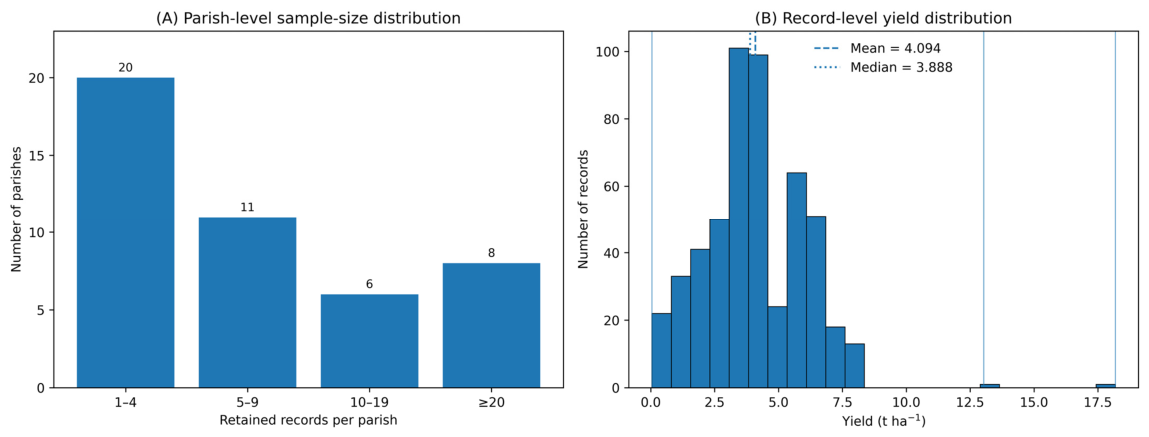
The 518 crop records corresponded to 433 unique producers and represented 45 parishes distributed across 18 cantons. The number of observations per parish ranged from 1 to 81, with a median of 5 records. The largest parish contributed 81 records (15.6% of the analytical sample), and the five most represented parishes jointly contributed 244 records (47.1%). The five parish-grouped outer assessment folds were closely balanced in total record count, containing 103 or 104 observations and between 8 and 10 parishes, but this did not imply equal geographical representation. In the most spatially unbalanced assessment fold, a single parish contributed 81 of 104 records (77.9%). The grouped design ensured that all records from the same parish—and consequently all records belonging to the same producer—remained within a single outer fold, while the unequal parish sizes were retained as an explicit feature of the observed sampling structure.

The five outer assessment folds also differed in their observed-yield distributions. Fold 1 contained 104 records from 8 parishes, with a mean yield of 4.201 t ha⁻¹, a median of 4.091 t ha⁻¹, and an interquartile range of 3.182–5.710 t ha⁻¹. Fold 2 contained 104 records from 9 parishes, with a mean of 3.763 t ha⁻¹, a median of 3.409 t ha⁻¹, and an interquartile range of 2.511–4.545 t ha⁻¹. Fold 3 contained 104 records from 10 parishes, with a mean of 3.791 t ha⁻¹, a median of 3.712 t ha⁻¹, and an interquartile range of 2.455–4.545 t ha⁻¹. Fold 4 contained 103 records from 9 parishes, with a mean of 4.276 t ha⁻¹, a median of 4.091 t ha⁻¹, and an interquartile range of 3.270–5.545 t ha⁻¹. Fold 5 contained 103 records from 9 parishes, with a mean of 4.442 t ha⁻¹, a median of 4.545 t ha⁻¹, and an interquartile range of 2.949–5.773 t ha⁻¹. The complete record-to-parish and parish-to-fold assignments are provided in the supplementary cross-validation file.

Three yield observations were flagged by the predefined plausibility audit: two in the upper tail and one close to zero. These observations were retained in the primary analysis but excluded from the strict sensitivity specification, which contained 515 records. A further climate-coverage sensitivity sample contained 492 records located in parishes with ERA5-Land valid-land coverage of at least 90%.

Table 3. Construction of the analytical sample and predefined sensitivity subsets.

Sample-Construction Stage or Analytical Subset	Records, n	Decision or Analytical Role
Hard dry maize records initially identified in Manabí	527	Initial crop- and province-specific extraction
Exact duplicate records	2	Excluded
Unique hard dry maize records	525	Retained after duplicate control
Associated-crop records	7	Separated because harvested area was not necessarily crop-specific
Principal sole-crop analytical sample	518	Primary descriptive and predictive analysis
Records linked to producer and land-unit information	518	Complete linkage
Records linked to complete CHIRPS3 and ERA5-Land crop-season series	518	Integrated survey-plus-climate analysis
Strict yield-plausibility sensitivity sample	515	Excluded two upper-tail and one near-zero observation
ERA5-Land coverage sensitivity sample	492	Restricted to valid-land coverage ≥ 90%

summarizes the sample-construction sequence and the analytical subsets.

Hard dry maize yield in the principal sample had an unweighted mean of 4.094 t ha⁻¹ and a survey-weighted mean of 4.087 t ha⁻¹. The median was 3.888 t ha⁻¹, with an interquartile range of 2.727–5.455 t ha⁻¹. Observed values ranged from 0.045 to 18.182 t ha⁻¹. The mean exceeded the median and a small number of comparatively high observations extended the upper tail, resulting in a moderately right-skewed distribution. The three most extreme observations were retained in the primary analysis in accordance with the predefined sample-construction rules.

Figure 1 shows the uneven distribution of observations across parishes and the empirical distribution of hard dry maize yield in the principal analytical sample.

Certified seed represented the largest seed category, accounting for 290 records and a survey-weighted proportion of 55.7%. Improved seed accounted for 30.8% of the weighted distribution, common seed for 12.7%, and the aggregated hybrid category for 0.8%. Manual or traditional soil preparation was the most common preparation category, with a weighted proportion of 48.5%, followed by other methods at 27.8%, mechanized preparation at 12.8%, and no reported preparation at 10.8%.

Irrigation was reported for 51 records, corresponding to a survey-weighted proportion of 7.5%. Drainage was considerably less frequent and was reported for only six records, equivalent to 1.1% of the weighted sample. Fertilizer use was reported for 94.1% of the weighted observations and crop-protection use for 94.4%.

The median planted maize area was 2.117 ha, with an interquartile range of 1.000–5.000 ha. The median total farm area was 7.379 ha, with an interquartile range of 3.440–16.000 ha. The substantially larger unweighted means of these variables reflected a small number of very large production units. The corresponding survey-weighted means were 3.594 ha for planted maize area and 13.792 ha for total farm area.

Producers had a median age of 56 years, with an interquartile range of 45–67 years. Men represented 85.6% of the survey-weighted sample. Primary or basic education was the predominant educational category, accounting for 69.0% of the weighted distribution, whereas 18.3% had secondary education, 1.9% higher education, and 10.8% no formal education. Rural social-security participation was reported for 43.4% of the weighted observations. Smartphone access was reported for 55.5%, Internet access for 27.7%, and computer access for 3.4%.

Table 4. Yield, farm-management, producer, and technological characteristics of the analytical sample.

Characteristic	Unweighted Sample Result	Survey-Weighted Estimate
Continuous variables
Yield, t ha−1	Mean: 4.094; median: 3.888; IQR: 2.727–5.455	Mean: 4.087
Planted maize area, ha	Median: 2.117; IQR: 1.000–5.000	Mean: 3.594
Total farm area, ha	Median: 7.379; IQR: 3.440–16.000	Mean: 13.792
Producer age, years	Median: 56; IQR: 45–67	Mean: 55.797
Seed type
Certified	290 (56.0%)	55.7%
Improved	168 (32.4%)	30.8%
Common	54 (10.4%)	12.7%
Hybrid	6 (1.2%)	0.8%
Soil preparation
Manual or traditional	227 (43.8%)	48.5%
Mechanized	91 (17.6%)	12.8%
None	52 (10.0%)	10.8%
Other	148 (28.6%)	27.8%
Water and input management
Irrigation use	51 (9.8%)	7.5%
Drainage use	6 (1.2%)	1.1%
Fertilizer use	493 (95.2%)	94.1%
Crop-protection use	484 (93.4%)	94.4%
Producer characteristics
Male	443 (85.5%)	85.6%
No formal education	51 (9.8%)	10.8%
Primary or basic education	340 (65.6%)	69.0%
Secondary education	91 (17.6%)	18.3%
Higher education	36 (6.9%)	1.9%
Rural social-security participation	207 (40.0%)	43.4%
Digital access
Computer access	26 (5.0%)	3.4%
Smartphone access	301 (58.1%)	55.5%
Internet access	157 (30.3%)	27.7%

Note: IQR, interquartile range. Percentages may not sum to exactly 100% because of rounding. Continuous weighted estimates are means calculated using the ESPAC final expansion factor.

presents the principal yield, farm, management, producer, and digital-access characteristics. Unweighted counts describe the empirical analytical sample, whereas the weighted percentages and means use the ESPAC final expansion factor.

Unadjusted yield distributions differed across several management categories. The median yield was 4.201 t ha⁻¹ for certified seed, 3.852 t ha⁻¹ for improved seed, and 2.164 t ha⁻¹ for common seed. The hybrid category had a median of 6.647 t ha⁻¹ but contained only six observations and was therefore not considered sufficiently represented for an independent substantive conclusion.

Irrigated records had a median yield of 4.306 t ha⁻¹, compared with 3.880 t ha⁻¹ among non-irrigated records. The median yield was 3.927 t ha⁻¹ among records reporting fertilizer use and 3.247 t ha⁻¹ among those not reporting fertilizer use. The corresponding medians for crop-protection use were 4.091 and 2.889 t ha⁻¹. These comparisons are descriptive only. They do not estimate isolated management effects because the management practices, farm characteristics, geographical conditions, and crop-season climate exposures were not independently assigned.

The complete climate database covered 427 consecutive days from 1 November 2023 to 31 December 2024. After parish-level aggregation, it contained 19,215 parish-day observations, corresponding to 45 parishes multiplied by 427 days. No parish-day values were missing from the variables used in the crop-season calculations.

The reported crop cycles began between November 2023 and October 2024 and ended between March and December 2024. The primary full-month exposure windows had a median duration of 182 days and an interquartile range of 160.25–213 days. Individual windows ranged from 90 to 275 days.

The median cumulative precipitation during the full-month crop window was 588.36 mm, with an interquartile range of 503.08–807.60 mm. Precipitation exposure varied markedly across records, ranging from 9.04 to 1924.26 mm. The median number of wet days with precipitation of at least 1 mm was 70, while the median longest consecutive dry spell was 25 days.

The mean crop-season air temperature showed substantially less variation than precipitation. The overall mean was 25.5 °C, and individual crop-window means ranged from 23.5 to 26.3 °C. The mean upper-layer volumetric soil moisture was 0.408 m³ m⁻³, with a range of 0.181–0.481 m³ m⁻³.

Table 5. Descriptive statistics for full-month crop-season climate exposure.

Variable	Mean	SD	Median	IQR	Minimum–Maximum
Crop-window duration, days	186.8	35.0	182.0	160.3–213.0	90.0–275.0
Cumulative precipitation, mm	694.0	388.4	588.4	503.1–807.6	9.0–1924.3
Wet days with precipitation ≥ 1 mm, days	74.1	24.7	70.0	67.0–88.0	2.0–143.0
Longest consecutive dry spell, days	24.4	14.0	25.0	16.0–26.0	3.0–82.0
Mean 2 m air temperature, °C	25.5	0.4	25.6	25.3–25.8	23.5–26.3
Mean upper-layer soil moisture, m3 m−3	0.408	0.053	0.422	0.39–0.443	0.181–0.481

Note: SD, standard deviation; IQR, interquartile range. Statistics are calculated across the 518 crop records using their corresponding full-month crop-season windows.

reports the complete descriptive statistics.

The spatial and temporal resolution of the linkage also resulted in repeated climate-exposure profiles among crop records. The 518 analytical records represented 166 unique combinations of parish and primary full-month crop window. Consequently, 420 records (81.1%) shared the same four final full-window climate predictor values with at least one other record, and the largest identical-exposure group contained 53 records. These repetitions do not represent duplicated agricultural observations; they arise because records with the same parish and crop window are linked to the same underlying parish-level daily climate series.

Cumulative precipitation and wet-day count were strongly correlated in every outer training partition. The absolute Spearman correlation ranged from 0.896 to 0.924 across the five folds, exceeding the prespecified threshold of 0.80. Wet-day count was consequently excluded from model fitting, while cumulative precipitation was retained as the principal rainfall-amount indicator. The integrated models therefore included cumulative precipitation, longest dry spell, mean air temperature, and mean soil moisture.

Valid ERA5-Land land-cell coverage was below 90% in Charapoto, Canoa, Montecristi, and Jama, affecting 26 records. These observations were retained in the primary analysis because complete daily parish-level series were available for every crop window. Their potential influence was evaluated through the predefined 492-record coverage sensitivity analysis.

4.2. Primary Spatial Prediction Performance

Table 6. Spatially grouped out-of-fold predictive performance in the primary analysis.

Predictor Configuration	Algorithm	MAE, t ha−1	Parish-Cluster 95% CI for MAE	RMSE, t ha−1	Out-of-Sample R2
Benchmark	Training-fold mean yield	1.534	1.384–1.712	1.979	−0.011
Survey only	Histogram-based gradient boosting	1.535	1.409–1.689	2.020	−0.053
Survey only	Random Forest	1.546	1.418–1.705	2.041	−0.076
Survey only	Elastic Net	1.550	1.419–1.717	2.034	−0.068
Survey plus climate	Histogram-based gradient boosting	1.548	1.420–1.701	2.033	−0.067
Survey plus climate	Random Forest	1.551	1.422–1.713	2.043	−0.077
Survey plus climate	Elastic Net	1.570	1.438–1.741	2.045	−0.079

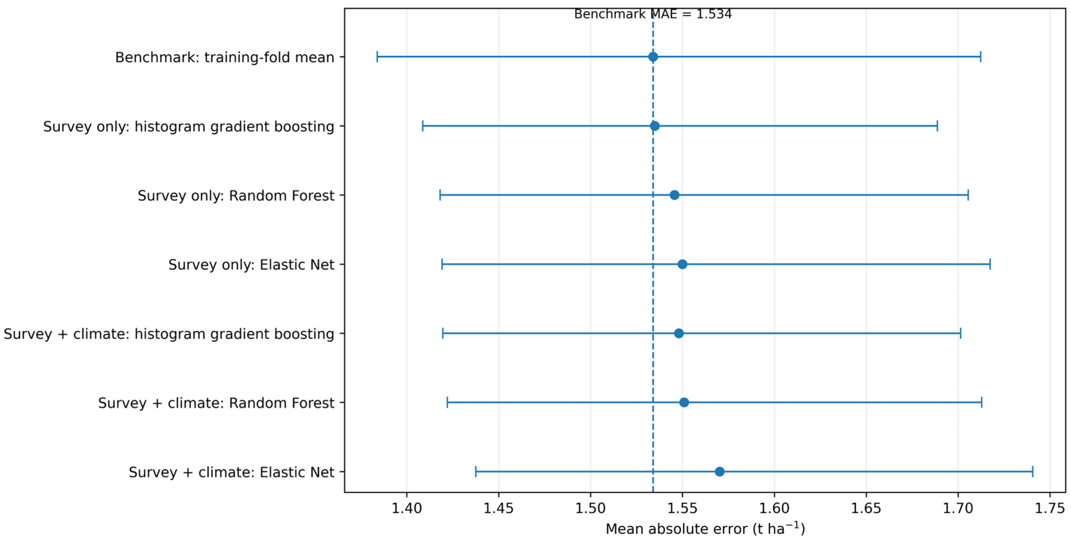
Note: MAE, mean absolute error; RMSE, root-mean-square error; CI, confidence interval. Metrics were calculated after pooling the out-of-fold predictions from the five parish-grouped outer assessment folds. Lower MAE and RMSE and higher R² indicate better predictive performance. Bold values identify the best result for each metric.

presents the pooled out-of-fold performance obtained under the primary five-fold parish-grouped validation design. The fold-specific mean-yield benchmark achieved an MAE of 1.534 t ha⁻¹, an RMSE of 1.979 t ha⁻¹, and a pooled out-of-sample R² of −0.011.

Among the survey-only models, histogram-based gradient boosting produced the lowest MAE at 1.535 t ha⁻¹. Random Forest and Elastic Net produced MAEs of 1.546 and 1.550 t ha⁻¹, respectively. The survey-only histogram-based gradient-boosting model was therefore the strongest-performing complex specification according to the primary metric, but its MAE remained 0.001 t ha⁻¹ higher than that of the benchmark. The corresponding relative difference represented a deterioration of approximately 0.06%. Given the negligible magnitude of this point difference, the comparison was not interpreted from the pooled MAE ranking alone but together with the benchmark-relative uncertainty interval and the consistency of performance across the five geographically separated assessment folds. The parish-cluster bootstrap interval for the benchmark-relative MAE improvement of the survey-only histogram-based gradient-boosting model ranged from −0.078 to 0.091 t ha⁻¹. The interval included zero and did not support a consistent predictive improvement. This model outperformed the benchmark in only two of the five outer folds.

All survey-plus-climate models also produced higher pooled MAE values than the benchmark. The strongest integrated specification was histogram-based gradient boosting, with an MAE of 1.548 t ha⁻¹, an RMSE of 2.033 t ha⁻¹, and an R² of −0.067. It outperformed the benchmark in only one of the five outer geographical folds.

Figure 2 visually compares the pooled MAE estimates and parish-cluster bootstrap intervals obtained under the primary spatially grouped validation design.

Across the five individual outer assessment folds, the survey-only histogram-based gradient-boosting model produced MAE values ranging from 1.402 to 1.737 t ha⁻¹. Its strongest relative results occurred in outer folds 1 and 2, where it improved on the corresponding fold-specific benchmark. In folds 0, 3, and 4, its MAE was higher than the benchmark. The variability across geographically separated assessment folds indicated that relationships learned from the training parishes did not transfer uniformly to the parishes withheld for assessment.

The pooled R² was negative for the benchmark and for every fitted model. Moreover, the complex models produced RMSE values between 2.020 and 2.045 t ha⁻¹, compared with 1.979 t ha⁻¹ for the benchmark. Because no complex model outperformed the benchmark while showing stable performance across the geographical folds, the prespecified condition for substantive model interpretation was not satisfied. Feature-importance, partial-dependence, threshold, and interaction outputs were therefore not interpreted as evidence of agronomic determinants.

4.3. Incremental Predictive Contribution of Climate Information

The addition of crop-season climate information did not improve primary predictive performance for any of the three algorithms. For Elastic Net, MAE increased from 1.550 to 1.570 t ha⁻¹. The corresponding climate-related MAE reduction, defined as survey-only MAE minus survey-plus-climate MAE, was −0.020 t ha⁻¹, equivalent to a relative deterioration of 1.31%. The parish-cluster 95% bootstrap interval ranged from −0.042 to −0.004 t ha⁻¹, and the climate-enhanced model did not improve MAE in any outer fold.

For Random Forest, the inclusion of climate indicators increased MAE from 1.546 to 1.551 t ha⁻¹. The resulting MAE reduction was −0.005 t ha⁻¹, equivalent to −0.34%, with a 95% bootstrap interval from −0.044 to 0.032 t ha⁻¹. Climate information improved Random Forest performance in two of the five folds but worsened or did not materially improve it in the remaining folds.

For histogram-based gradient boosting, MAE increased from 1.535 to 1.548 t ha⁻¹ after the climate indicators were added. The absolute MAE reduction was −0.013 t ha⁻¹ and the relative reduction was −0.85%. The parish-cluster 95% bootstrap interval ranged from −0.061 to 0.036 t ha⁻¹. The integrated specification improved on its survey-only counterpart in two outer folds but produced higher error in the other three.

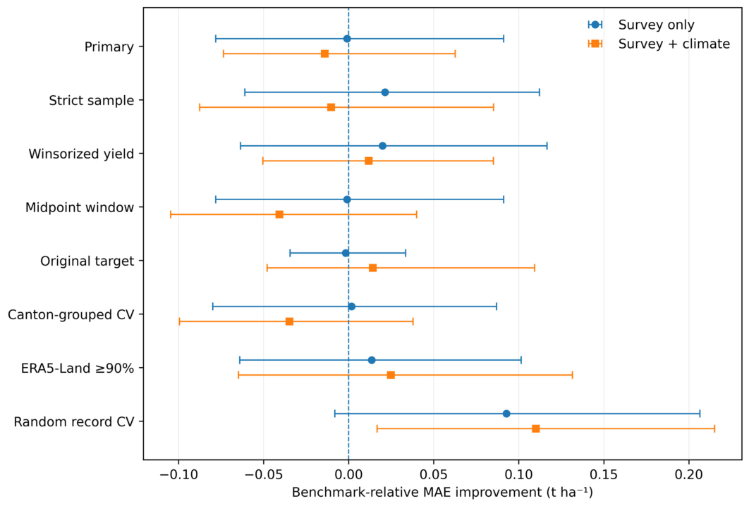
The best integrated model also remained 0.014 t ha⁻¹ worse than the mean-yield benchmark. Its benchmark-relative improvement interval ranged from −0.074 to 0.063 t ha⁻¹. Crop-season precipitation, dry-spell duration, temperature, and soil moisture therefore provided no consistent incremental predictive value beyond the survey variables under the primary parish-grouped validation design.

4.4. Robustness of the Negative Predictive Finding

Table 7. Robustness of predictive performance across alternative specifications.

Specification	n	Benchmark MAE	Survey-Only MAE	Survey-Plus-Climate MAE	Climate-Related ΔMAE, t ha−1 (%)	Outer Folds Improved by Climate
Primary: full-month window, log-transformed target, parish grouping	518	1.534	1.535	1.548	−0.013 (−0.85%)	2 of 5
Strict yield-plausibility sample	515	1.485	1.464	1.496	−0.032 (−2.16%)	1 of 5
Yield winsorized at the 1st and 99th percentiles	518	1.501	1.481	1.489	−0.008 (−0.55%)	3 of 5
Midpoint-based crop window	518	1.534	1.535	1.575	−0.040 (−2.59%)	0 of 5
Original, untransformed target scale	518	1.534	1.536	1.520	+0.016 (+1.04%)	2 of 5
Canton-grouped validation	518	1.539	1.537	1.573	−0.037 (−2.38%)	1 of 5
ERA5-Land valid-land coverage ≥ 90%	492	1.474	1.461	1.449	+0.011 (+0.77%)	2 of 5
Random record-level cross-validation	518	1.528	1.435	1.418	+0.017 (+1.21%)	4 of 5

Note: ΔMAE = MAE of the survey-only model minus MAE of the survey-plus-climate model. Positive values indicate lower error after climate information was added. The random record-level specification is diagnostic and is not treated as the preferred estimate of geographical transferability.

compares the primary histogram-based gradient-boosting results with the predefined alternative specifications. The alternative analyses changed the outcome treatment, crop-season window, target scale, geographical grouping structure, climate-coverage criterion, or cross-validation design. Positive climate-related MAE reductions indicate that climate information reduced prediction error, whereas negative values indicate that it increased error.

Paired 95% cluster-bootstrap intervals for the survey-only and survey-plus-climate benchmark-relative MAE differences and for the incremental climate-related MAE difference across all robustness specifications are reported in Supplementary File S10 and summarized graphically in Figure 3.

Figure 3 summarizes the benchmark-relative performance of the survey-only and survey-plus-climate histogram-based gradient-boosting models across the primary and robustness specifications.

Removing the three observations flagged by the strict yield-plausibility audit reduced the survey-only MAE to 1.464 t ha⁻¹, which was 0.021 t ha⁻¹ lower than the corresponding benchmark. However, the addition of climate information increased MAE to 1.496 t ha⁻¹. Similarly, after winsorization, the survey-only and integrated models achieved MAEs of 1.481 and 1.489 t ha⁻¹, respectively, compared with 1.501 t ha⁻¹ for the benchmark. The small MAE advantages observed in these outcome-sensitivity analyses were not accompanied by positive pooled R² values and did not establish consistent climate-related improvement. The benchmark-relative uncertainty intervals qualify the interpretation of the point estimates in Table 7. Under the spatially structured robustness specifications, the 95% intervals for the survey-plus-climate model relative to the corresponding benchmark included zero, including the original-target specification (+0.014 t ha⁻¹; 95% CI: −0.048 to 0.109) and the ERA5-Land ≥ 90% specification (+0.025 t ha⁻¹; 95% CI: −0.065 to 0.132). These results therefore indicate a lack of clear evidence for benchmark-relative improvement rather than evidence that improvement was absent. In contrast, under random record-level cross-validation, the survey-plus-climate model improved on the benchmark by 0.110 t ha⁻¹ (95% CI: 0.017 to 0.215). This improvement is supported within the random-record assessment design but cannot be interpreted as evidence of geographical transferability.

Replacing the full-month crop window with the midpoint-based window produced the least favourable integrated result. Survey-plus-climate MAE increased to 1.575 t ha⁻¹, and climate information failed to improve performance in any of the five folds. Because direct original-scale modelling does not require retransformation, this sensitivity analysis provides a direct check on whether the primary finding depended on the log-transformed target. Under this specification, the histogram-based gradient-boosting survey-only model achieved an MAE of 1.536 t ha⁻¹ and the survey-plus-climate model achieved 1.520 t ha⁻¹, compared with 1.534 t ha⁻¹ for the benchmark. Climate information therefore reduced MAE by 0.016 t ha⁻¹ (1.04%), but the improvement occurred in only two of five outer folds and the integrated model retained a negative pooled R² of −0.024. The target scale therefore affected the direction of the small estimated climate contribution but did not establish stable predictive improvement under geographical transfer.

Under canton-grouped validation, the survey-only MAE of 1.537 t ha⁻¹ was close to the benchmark value of 1.539 t ha⁻¹, whereas the survey-plus-climate MAE increased to 1.573 t ha⁻¹. Restricting the sample to the 492 records with ERA5-Land valid-land coverage of at least 90% produced an integrated MAE of 1.449 t ha⁻¹, compared with 1.461 t ha⁻¹ for the survey-only model and 1.474 t ha⁻¹ for the benchmark. This represented a small climate-related improvement, but it occurred in only two of the five folds and the pooled R² remained negative at −0.013.

The diagnostic random record-level cross-validation specification produced substantially more favourable results. Under this design, the survey-only model achieved an MAE of 1.435 t ha⁻¹ and the survey-plus-climate model achieved an MAE of 1.418 t ha⁻¹, compared with 1.528 t ha⁻¹ for the random-split benchmark. The integrated model therefore reduced MAE by approximately 0.110 t ha⁻¹, or 7.2%, relative to the benchmark, and produced a small positive pooled R² of 0.024.

This apparent improvement disappeared when entire parishes were withheld from model development. The contrast between random and spatially grouped validation indicates that record-level random partitions produced a more optimistic assessment because records from the same or environmentally similar geographical contexts could be represented in both training and assessment samples.

Overall, the robustness analyses did not identify a stable specification in which the complex model consistently outperformed the benchmark across geographically separated assessment groups. Climate information produced small improvements under the original-target, high-coverage, and random record-level specifications, but these improvements were not reproduced under the primary, strict-sample, winsorized, midpoint-window, or canton-grouped designs. The principal conclusion therefore remained unchanged: the observed survey and crop-season climate variables did not support reliably transferable farm-record-level yield prediction for hard dry maize in parishes not represented during model development.

5. Discussion

This study examined whether farm-management, producer, and crop-season climate information could support out-of-sample prediction of hard dry maize yield in Manabí Province, with particular emphasis on transferability to parishes not represented during model development. The Discussion is organized around four findings. First, the analytical sample contained substantial variation in yield, farm-management characteristics, spatial representation, and climate exposure, but the available information also presented important limitations in measurement granularity and geographical resolution. Second, none of the evaluated machine-learning models provided stable predictive improvement over the fold-specific mean benchmark under parish-grouped validation. Third, adding crop-season climate indicators did not produce a consistent incremental reduction in prediction error. Fourth, the principal negative finding remained broadly stable across the predefined robustness analyses, whereas substantially more favourable performance under random record-level validation indicated sensitivity to geographical structure.

These findings do not imply that farm management or climate is unrelated to maize yield. Rather, they indicate that the available survey and parish-level climate variables did not contain sufficiently stable and spatially resolved information to generate reliable predictions for farms located in previously unseen parishes. The following subsections discuss each of these findings in the same sequence in which they are presented in the Section 4 .

5.1. Sample Characteristics and Information Constraints

The analytical sample combined complete survey–climate linkage with substantial variation in observed yield, farm-management practices, producer characteristics, and environmental exposure. However, descriptive heterogeneity should not be equated with transferable predictive information. Reliable prediction for unseen geographical areas additionally requires predictors that represent relevant production processes with sufficient spatial, temporal, and measurement resolution.

The descriptive analysis identified yield differences across seed, irrigation, fertilizer, and crop-protection categories. Certified-seed records, for example, had a higher median yield than common-seed records, while records reporting irrigation, fertilizer use, or crop-protection use also tended to present higher median yields than their corresponding comparison categories.

These differences are potentially relevant for hypothesis development but cannot be interpreted as causal effects. Management practices were not randomly assigned, and producers adopting a particular practice may differ systematically in farm size, financial resources, soil quality, market access, technical assistance, geographical location, production objectives, or other unobserved characteristics. A higher median yield among users of an input therefore does not establish the yield increase attributable to that input.

Measurement granularity also constrained the predictive contribution of the survey variables. Fertilizer and crop-protection practices were represented by indicators identifying whether any product was used. The original quantities could not be harmonized consistently because producers reported inputs using heterogeneous units. Consequently, the models could distinguish users from non-users but could not represent application rate, formulation, timing, frequency, or nutrient composition.

Similar limitations apply to irrigation. The principal model identified whether irrigation was used but did not represent the volume of water applied, irrigation scheduling, system efficiency, or whether irrigation occurred during a critical development stage. The modest unadjusted median-yield difference between irrigated and non-irrigated records should therefore not be interpreted as the expected agronomic effect of irrigation. Only 51 of the 518 records reported irrigation, and the observed difference may also reflect rainfall distribution, production environment, genetic material, and broader differences in management intensity between irrigated and non-irrigated farms. The reported ESPAC seed category was available, but detailed cultivar or hybrid identity and maturity class were not represented.

The weak spatial performance of the survey-only models therefore does not demonstrate that management has no relationship with yield. It indicates that the available survey representations of management, producer, and farm characteristics were insufficient to predict yield reliably across unseen parishes. Predictive modelling cannot recover information that was not collected or was measured too broadly to distinguish agronomically meaningful differences.

5.2. Primary Spatial Prediction Performance and Transferability

The survey-only histogram-based gradient-boosting model produced the lowest MAE among the complex specifications, but its error was virtually identical to—and marginally higher than—that of the benchmark. Random Forest and Elastic Net also failed to improve on the benchmark, and all complex models produced negative pooled out-of-sample R² values. The observed predictor–yield relationships therefore did not generalize consistently across geographically separated assessment folds. The agreement across these different model classes reduces, but does not eliminate, the possibility that the negative finding reflects a particular hyperparameter configuration; the randomized search was deliberately bounded and should not be interpreted as an exhaustive optimization of the three algorithms.

This pattern is more consistent with a limitation in information content and spatial transferability than with the failure of a particular algorithm. Although the analytical sample contained 518 records, spatial transfer was evaluated across only 45 parishes, and the number of records per parish was highly unbalanced, ranging from 1 to 81 with a median of 5. Consequently, the amount of geographically distinct information available for learning relationships that persist across locations was considerably smaller than the record count alone might suggest. The fact that a regularized linear model and two nonlinear tree-based ensemble models all produced performance close to or worse than the same benchmark further indicates that the measured predictors contained weak or unstable transferable signal, rather than simply reflecting misspecification of a single model class.

The negative predictive result may therefore arise from several non-exclusive mechanisms. Spatial heterogeneity can produce parish-specific relationships between management, environmental conditions, and yield, while withholding entire parishes can introduce distributional differences between training and assessment data that are largely absent under random record-level partitioning. At the same time, survey-derived production and management variables remain subject to reporting and measurement error, and several management inputs are represented only through relatively coarse use/non-use indicators. Parish-level climate assignment and crop windows reconstructed from reported months introduce additional spatial aggregation and temporal measurement error that may attenuate farm-level predictor–yield relationships. These mechanisms cannot be separated statistically with the present single-year public-use dataset, which lacks field coordinates and repeated observations across production years. The model failure should therefore be interpreted as evidence that the combined information content, measurement detail, and spatial-temporal resolution of the available predictors were insufficient for stable transfer to unseen parishes, rather than as evidence that management or climate is intrinsically unrelated to maize yield.

The contrast between spatially grouped and random record-level validation provides direct evidence of this problem. Under random cross-validation, the integrated histogram-based gradient-boosting model achieved an MAE of 1.418 t ha⁻¹, compared with 1.528 t ha⁻¹ for the corresponding benchmark, and produced a small positive pooled R². Under parish-grouped validation, however, its MAE increased to 1.548 t ha⁻¹ and no longer improved on the benchmark.

Random record-level partitions allow observations from the same parish, or from parishes with closely related production and environmental characteristics, to occur in both the training and assessment samples. Models can then exploit shared local structures that would not be available when predicting in a genuinely unobserved location. Roberts et al. [6] emphasize that cross-validation must reflect the spatial, temporal, or hierarchical structure of the intended prediction problem. Similarly, Radočaj et al. showed that regular and spatial cross-validation can produce materially different assessments of maize-yield prediction [7].

The present comparison also reinforces the importance of preventing indirect information leakage. Although no outcome-derived variables were used and all preprocessing was restricted to the corresponding training folds, geographical proximity itself can create an optimistic assessment when spatially related observations are distributed across training and assessment partitions. This form of structural dependence is consistent with the broader leakage concerns discussed by Kaufman et al. [26].

The primary parish-grouped results should therefore be regarded as the more credible estimate of the form of spatial transferability examined in this study. They answer the operationally relevant question of whether relationships learned from surveyed farms in one group of parishes can be applied to farms in other parishes. For the variables and sample evaluated here, the answer was negative.

This finding does not contradict the broader literature showing that machine-learning algorithms can support crop-yield prediction. Reviews such as Van Klompenburg et al. [16] demonstrate that predictive performance depends strongly on the crop, geographical scale, predictor resolution, sample size, study period, remote-sensing availability, and validation strategy. Studies using richer temporal data, field-specific soil information, remotely sensed crop development, or repeated observations may capture production signals that are unavailable in a single-year agricultural survey.

Comparisons with studies such as Kouame et al. [17], Kumar et al. [18], and Sihi et al. [19] should therefore be made cautiously. These studies differ substantially in their geographical context, observation scale, predictor sources, and prediction objectives. Their results do not establish that the same level of predictability should be expected from anonymized parish-linked survey records in Manabí.

5.3. Incremental Contribution of Climate Information

The inclusion of climate indicators did not consistently improve prediction for any of the three algorithms. In the primary specification, the integrated models produced higher MAE values than their corresponding survey-only models. The deterioration was small for Random Forest and histogram-based gradient boosting but was observed consistently enough to reject the proposition that the selected climate variables provided a clear incremental predictive gain.

The apparently favourable climate results under selected robustness specifications can be examined more specifically because the alternative analyses changed different components of the modelling design. When yield was fitted directly on its original scale, the analytical sample, parish grouping, and climate information remained unchanged; the principal change was the target scale on which the model was fitted. Under this specification, climate reduced MAE by only 0.016 t ha⁻¹ (1.04%) and improved performance in two of five folds, while pooled R² remained negative. The small gain therefore indicates sensitivity of the estimated incremental climate contribution to target transformation and model fitting rather than evidence that a stronger or more transferable climate signal had been recovered.

The ERA5-Land coverage sensitivity has a different interpretation. Restricting the analysis to the 492 records with valid-land coverage of at least 90% simultaneously changed sample composition and removed records from the four lower-coverage coastal parishes. Importantly, the benchmark MAE decreased from 1.534 to 1.474 t ha⁻¹ and the survey-only model MAE decreased from 1.535 to 1.461 t ha⁻¹ before any incremental climate advantage was considered. Climate then reduced MAE by a further 0.011 t ha⁻¹ and improved two of the five folds, but pooled R² remained negative. Because the restriction changed both the observations being predicted and the quality criterion applied to the ERA5-Land linkage, the small climate improvement cannot be attributed uniquely to better climate-data quality; a change in sample composition and fold composition also contributed to the different performance context.

The spatial resolution of the climate linkage may also have constrained the detectable incremental signal. Although 518 crop records were analysed, they represented only 166 unique parish–crop-window exposure profiles, and 420 records (81.1%) shared the same four final climate predictor values with at least one other record. Consequently, yield differences associated with local rainfall, elevation, coastal exposure, soil-water conditions, or other within-parish environmental variation could occur without corresponding differences in the climate predictors. This spatial mismatch may therefore have attenuated the farm-record-level climate–yield signal and contributed to the weak and unstable predictive benefit of the integrated models.

Temporal aggregation provides a second potential source of signal attenuation. The primary windows summarized climate conditions over periods ranging from 90 to 275 days, whereas maize sensitivity to rainfall, heat, and soil-water availability may be concentrated within substantially shorter developmental stages. Whole-season cumulative or mean indicators can therefore combine conditions occurring during agronomically critical periods with conditions occurring during less sensitive stages, potentially weakening their relationship with final yield. The midpoint sensitivity did not recover a stronger climate contribution, but it altered only the calendar boundaries of the exposure window and did not identify flowering, pollination, or grain-filling periods. A genuinely phenology-aligned analysis would require exact planting dates, observed developmental stages, or sufficiently detailed cultivar and maturity information, none of which is available in the ESPAC public-use records. Imposing standardized stage windows without this information would introduce unverified assumptions rather than reduce exposure uncertainty.

The random record-level specification provides clearer evidence concerning spatial dependence because it retained the same 518 records, target transformation, and climate variables while changing the validation structure. Under random validation, climate reduced MAE by 0.017 t ha⁻¹ and improved four of five folds, while the integrated model reduced MAE by approximately 0.110 t ha⁻¹ relative to the benchmark. This improvement disappeared when entire parishes were withheld. The contrast is therefore consistent with climate and survey predictors being more useful for interpolation among records drawn from already represented geographical contexts than for transfer to previously unseen parishes.

The absence of incremental predictive improvement must not be interpreted as evidence that weather and soil-water conditions are agronomically unimportant. Previous research has demonstrated that maize production can be affected by drought, extreme heat, and excessive rainfall [13,14,15]. Climate-related yield effects have also been reported in southwestern Ecuador [3]. The present results address a narrower question: whether four climate indicators, calculated from parish-level gridded data over survey-derived crop windows, improved prediction beyond the available farm and producer variables.

Several factors may explain the limited predictive contribution. First, the study covered one ESPAC survey year and therefore did not include the interannual climate variability that is often essential for identifying climate–yield relationships. Many influential climate effects become more detectable when the same regions are observed across contrasting seasons, including unusually dry, wet, cool, or hot years.

Second, the temperature distribution was relatively compressed. The mean crop-season temperature varied less across records than cumulative precipitation or dry-spell duration. Limited predictor variation reduces the ability of a model to distinguish systematic temperature-related yield responses, even when temperature is agronomically relevant over a broader climatic range.

Third, climate exposure was assigned at parish level because the ESPAC public-use records do not disclose farm coordinates. Area-weighted parish estimates avoid arbitrary single-cell assignment and account explicitly for the spatial overlap between grid cells and parish polygons, but they inevitably smooth environmental variation within each administrative unit. All farms within a parish draw from the same underlying daily climate series, with record-level differences arising only when their reported crop windows differ. Consistent with this limitation, the 518 records generated only 166 unique parish–full-window climate profiles, and 420 records (81.1%) shared their four final climate predictor values with at least one other record. This aggregation reduces the effective environmental resolution of the crop-record-level analysis and can attenuate or obscure climate–yield relationships when fields within the same parish experience different rainfall, temperature, elevation, soil-water, or microclimatic conditions. It should therefore be interpreted as aggregation-induced exposure uncertainty rather than as evidence that climatic conditions are homogeneous within parishes.

Fourth, sowing and harvesting information was reported only by month. The primary full-month window was therefore chosen as the least assumption-dependent representation of crop-season exposure, while the midpoint window provided a shorter alternative without imposing unobserved phenological dates. The midpoint specification shortened the exposure period by approximately 29–30 days, but climate information performed less favourably under this specification: MAE increased by 0.040 t ha⁻¹ after climate variables were added, and no outer fold improved. Thus, simple shortening of the calendar window did not recover a stronger climate signal in these data. This result does not rule out stronger prediction from genuinely phenology-aligned exposure windows. Flowering, pollination, and grain filling may respond differently to heat or water stress, but constructing such windows credibly would require exact crop-calendar information, cultivar or maturity information, field observations, or remotely sensed phenological indicators that were unavailable in the present public-use dataset.

Fifth, the climate variables may have interacted with unobserved farm characteristics. Rainfall and soil moisture do not affect all fields equally; their consequences depend on soil texture, drainage, slope, cultivar, planting density, fertilizer availability, pest pressure, crop phenology, and the timing of management operations. These variables were either unavailable or insufficiently harmonized in the public-use survey files.

Finally, the selected climate indicators summarize broad crop-season exposure rather than event timing or physiological stress. Cumulative rainfall, longest dry spell, mean temperature, and mean upper-layer soil moisture do not explicitly represent rainfall intensity, waterlogging episodes, consecutive hot days, vapour-pressure deficit, or the timing of stress relative to crop development. Future studies combining field-level spatial information with exact or remotely sensed phenology could therefore evaluate whether stage-specific environmental indicators provide predictive information that is not recoverable from the whole-season summaries used here.

5.4. Robustness of the Negative Finding and Conditional Interpretation

The robustness analyses reinforced the primary conclusion rather than identifying a consistently superior alternative specification. Survey-only performance occasionally improved relative to the corresponding benchmark under selected outcome-sensitivity analyses, and small climate-related improvements appeared under the original-target, high-ERA5-coverage, and random record-level specifications. However, these advantages were not reproduced consistently across geographically separated folds or across the full set of analytical alternatives. The central negative predictive finding was therefore broadly robust to the predefined analytical changes, although the specification-specific variation reported in Table 7 remains relevant to its interpretation.

The uncertainty intervals provide an important qualification to this robustness pattern. Under the geographically structured specifications, several point estimates favoured either the survey-only or survey-plus-climate model, but the corresponding benchmark-relative 95% intervals included zero. These results should therefore be interpreted as a lack of clear evidence for benchmark-relative improvement, rather than as evidence that improvement was absent. The random record-level specification was the main exception: the survey-plus-climate model improved on the corresponding benchmark by 0.110 t ha⁻¹ (95% CI: 0.017 to 0.215). However, the incremental climate-related difference under the same specification was only 0.017 t ha⁻¹ (95% CI: −0.025 to 0.059), and random record-level validation does not test prediction in geographically unseen parishes. Thus, the additional uncertainty analysis does not alter the primary conclusion regarding spatial transferability, but it avoids the stronger and unsupported interpretation that predictive improvement is absent under every alternative analytical specification.

The target-scale sensitivity is particularly relevant to interpretation of the primary log-transformed specification. Direct inversion of a prediction fitted on ln(1 + Y) is not equivalent, in general, to a bias-corrected estimate of the conditional arithmetic mean on the original scale. The primary back-transformation should therefore not be interpreted as correcting retransformation bias. However, fitting the same prediction problem directly on the original yield scale removed this issue and produced only a small climate-related MAE improvement of 0.016 t ha⁻¹, with improvement in two of five folds and negative pooled R². The central finding is therefore not attributable solely to retransformation of the log-scale predictions, although the direction of the small climate-related difference was sensitive to target specification.

The study prespecified that feature importance and nonlinear response patterns would be interpreted only if a complex model improved on the benchmark and demonstrated reasonably stable performance across the outer folds. Because this condition was not satisfied, no agronomic interpretation was assigned to feature rankings, partial-dependence curves, thresholds, or interaction outputs.

This decision is methodologically important. Explainability techniques can describe how a fitted model generated its predictions, but they do not establish that the model learned a stable or externally valid relationship. A model with weak out-of-sample performance can still produce visually persuasive importance rankings and response curves. Interpreting those outputs as agronomic evidence would risk assigning substantive meaning to unstable associations.

Methods such as SHAP can provide coherent local and global explanations for tree-based models [20], and they have been used productively in crop-yield studies with stronger predictive foundations [18,19]. However, explainability does not compensate for insufficient predictive validity. Model interpretation should follow, rather than replace, evidence that the model generalizes to the intended prediction context.

The conditional interpretation rule therefore prevented overstatement of the findings. It also separates the present study from analyses that select the best-performing algorithm from a group of weak models and then interpret its predictors without first determining whether it improves on a meaningful benchmark.

5.5. Implications for Yield-Prediction Systems

The results have several implications for the development of agricultural decision-support systems in Manabí and comparable data-constrained settings. First, evaluation should be aligned with the intended deployment context. A model intended to estimate yield in farms or locations not represented during training must be assessed using geographical separation. Random cross-validation may be appropriate for interpolation among similar observations, but it should not be presented as evidence of spatial transferability.

Second, simple benchmarks should remain an explicit component of model assessment. The near-equivalence between the strongest complex model and the training-fold mean shows that algorithm rankings alone can be misleading. Selecting the lowest-MAE machine-learning model would have suggested that histogram-based gradient boosting was preferable, but comparison with the benchmark demonstrated that its apparent advantage was not operationally meaningful.

The methodological contribution therefore extends beyond the established observation that random validation can produce optimistic estimates. The combined use of geographical withholding, an explicit benchmark, paired evaluation of the incremental climate contribution, and predefined robustness analyses makes it possible to distinguish a lower error among competing algorithms from evidence of genuinely transferable predictive information.

Third, the current models should not be used as an operational farm-record-level yield-prediction tool Their error and instability across unseen parishes are too high to support individual production decisions, resource allocation, crop-insurance assessment, or farm-specific advisory recommendations.

Fourth, improving the algorithms without improving the information base is unlikely to resolve the principal limitation. The study already compared regularized linear and nonlinear ensemble models. Their similar inability to outperform the benchmark suggests that the primary constraint was not the absence of a more complex algorithm but the limited spatial and temporal representation of the underlying production system.

A stronger future prediction system would require multiple production years, precise farm or field coordinates under appropriate confidentiality safeguards, exact planting and harvesting dates, cultivar identity, soil characteristics, elevation and terrain, detailed input quantities and timing, irrigation schedules, pest and disease information, and repeated within-season remote-sensing observations. Combining survey data with field boundaries, crop phenology, vegetation indices, soil maps, and stage-specific weather indicators may allow the models to distinguish farms more effectively.

Hierarchical or spatially explicit models may also be appropriate when repeated data become available. Such approaches could separate farm-, parish-, canton-, and year-level variability and quantify the extent to which relationships are locally specific. Independent temporal validation should then be added to geographical validation to determine.

5.6. Strengths and Limitations

A principal strength of the study was the use of a fully traceable sample-construction process. Exact duplicates, associated-crop records, the principal sole-crop sample, and the strict plausibility sample were preserved as distinct analytical categories. Unusually high or low yields were not deleted solely because they were statistically extreme, and their influence was assessed through predefined robustness specifications.

A second strength was the integration of complete daily climate series. All 518 principal records were linked successfully to CHIRPS3 and ERA5-Land over their reconstructed crop windows, and no missing parish-day values occurred in the indicators used for analysis. The use of area-weighted grid–parish intersections provided a more defensible spatial assignment than arbitrary nearest-cell matching.

A third strength was the validation design. Preprocessing, correlation screening, hyperparameter selection, and model fitting were confined to the corresponding training data. Outer folds were grouped by parish, inner tuning folds retained the same grouping principle, all algorithms used common outer partitions, and a fold-specific benchmark was evaluated using the same observations. Parish-cluster bootstrap intervals and multiple robustness specifications provided additional information about uncertainty and result stability.

The study nevertheless has important limitations. The analysis was based on a single cross-sectional ESPAC survey year. It cannot determine whether the fitted relationships would remain stable across years with different rainfall, temperature, input prices, pest pressure, seed availability, or production conditions. Temporal external validation was therefore not possible.

The sample contained 518 records across 45 parishes, but the spatial sampling structure was highly unbalanced, with parish sample sizes ranging from 1 to 81 records and a median of 5. The largest parish represented 15.6% of the complete analytical sample, while the five largest parishes jointly represented 47.1%. Consequently, pooled record-level performance metrics give greater numerical influence to heavily represented parishes than to parishes represented by only one or a few records. This weighting is consistent with the record-level predictive estimand used in the study, but the resulting metrics should not be interpreted as an equally weighted average of predictive performance across parishes. This imbalance affects the reported metrics in different ways. MAE gives proportionally greater influence to parishes contributing more assessment records, while RMSE has the same record weighting but additionally gives greater influence to large individual residuals. Pooled R² depends on both prediction error and the variance of observed yield across the combined assessment records and can therefore also be affected by unequal parish representation and differences in yield distributions among folds. The three metrics should consequently be interpreted as record-level measures of predictive performance rather than as equally weighted measures of performance across geographical units.

The five primary assessment folds were nearly identical in total record count but necessarily differed in their geographical composition because of the unequal parish sizes. In the most spatially unbalanced assessment fold, a single parish contributed 81 of 104 records (77.9%). Fold-specific performance may therefore be influenced by the yield distribution and predictor structure of one or more highly represented parishes. Moreover, parish grouping prevents direct within-parish leakage but does not guarantee complete spatial independence, because neighbouring parishes may share environmental and production characteristics across administrative boundaries. A distance-based spatial blocking design could not be implemented because field coordinates are not available in the ESPAC public-use data.

The primary five-fold parish allocation was not repeated across multiple alternative allocations of the 45 parishes; therefore, some sensitivity to the exact composition of the assessment folds cannot be excluded. The parish-cluster bootstrap intervals preserve within-parish dependence and quantify variation in performance associated with the composition of the assessment parishes, conditional on the realized out-of-fold predictions. They do not represent uncertainty from repeated model fitting, hyperparameter selection, preprocessing estimation, or alternative outer-fold assignments. Spatial sensitivity was instead examined directly through the predefined canton-grouped nested cross-validation analysis. Under this coarser geographical grouping, the survey-only histogram-based gradient-boosting model remained essentially equivalent to the benchmark (MAE 1.537 versus 1.539 t ha⁻¹), while the survey-plus-climate model performed less favourably (MAE 1.573 t ha⁻¹). Thus, changing the geographical grouping level did not alter the central conclusion, although sensitivity to alternative allocations of parishes within the primary grouping level cannot be completely excluded.

The absence of farm coordinates required climate assignment at parish level. These exposure estimates do not measure the conditions experienced at the exact field location and cannot represent within-parish variation. This aggregation may reduce the detectable farm-level climate signal when substantial environmental heterogeneity exists within a parish. Four coastal parishes also had ERA5-Land valid-land coverage below 90%, although excluding their records did not change the central conclusion.

The crop-season windows were reconstructed from reported sowing and harvesting months rather than exact dates. The primary and midpoint specifications quantified part of this uncertainty but could not align climate exposure with specific maize-development stages. The midpoint analysis evaluated uncertainty in calendar-window boundaries, not phenological-stage exposure. Likewise, the upper-layer ERA5-Land soil-moisture indicator is a modelled reanalysis variable and should not be interpreted as a direct field measurement of root-zone water availability.

Yield was calculated from the standardized production and harvested-area variables available in ESPAC. Although these variables were internally audited and inconsistent observations were flagged, survey-derived production information may still contain reporting or measurement error. The public-use files also lacked several variables likely to influence maize yield, including detailed soil properties, cultivar identity, planting density, input rates, application timing, field-level pest severity, and technical-assistance intensity.

The models were designed for prediction rather than causal inference. No estimated difference, model coefficient, descriptive contrast, or climate contribution should therefore be interpreted as the causal effect of a management practice or environmental exposure. Survey expansion weights were used for population-oriented descriptive estimates but were not incorporated into model fitting, because the primary objective was out-of-sample prediction within the available analytical sample rather than design-based estimation of a population regression function.

Finally, the results are specific to hard dry maize production in Manabí and to the variables and period represented by ESPAC 2024. Generalization to other Ecuadorian provinces, crop types, years, or production systems requires independent evaluation. Importantly, the available evidence does not support attributing the negative predictive result to any single limitation. Rather, limited and uneven spatial representation, local heterogeneity, coarse predictor measurement, parish-level environmental aggregation, and differences between training and assessment locations may have acted jointly to reduce transferable predictive signal.

6. Conclusions

This study evaluated whether agricultural-survey characteristics and crop-season climate indicators could support transferable farm-record-level prediction of hard dry maize yield in Manabí Province, Ecuador. The analysis integrated 518 sole-crop ESPAC 2024 records with complete parish-level CHIRPS3 precipitation and ERA5-Land temperature and soil-moisture series, using geographically grouped nested cross-validation to assess performance in parishes excluded from model development.

The first objective was to determine whether machine-learning models based on survey-derived predictors could outperform the fold-specific mean-yield benchmark under parish-grouped validation; none of the evaluated algorithms did so. The survey-only histogram-based gradient-boosting model achieved the lowest MAE among the complex specifications, but its error remained marginally higher than that of the benchmark. Random Forest and Elastic Net also produced higher prediction errors, and all complex models presented negative pooled out-of-sample R² values.

The second objective examined whether crop-season climate information added predictive value beyond the survey-derived predictors; the inclusion of cumulative precipitation, longest dry-spell duration, mean air temperature, and mean upper-layer soil moisture did not provide a consistent incremental advantage. Small improvements appeared under selected alternative specifications, but they were not stable across geographical folds or reproduced across the full set of robustness analyses. Crop-season climate information therefore did not overcome the limited transferability of the available farm and management variables.

The third objective assessed the robustness of these findings across alternative analytical specifications; none of the predefined sensitivity analyses consistently changed the central conclusion. The contrast between random record-level and geographically grouped validation was particularly important. Random cross-validation produced apparently favourable performance, including a reduction in MAE relative to the benchmark. This improvement disappeared when entire parishes were withheld from training. The result demonstrates that random partitioning would have overstated the ability of the models to generalize to new geographical areas.

Because benchmark-relative predictive skill was not established under parish-grouped validation, model-explanation outputs were not interpreted as agronomic evidence.

The findings should not be understood as showing that management or climate is unimportant for maize production. Instead, they demonstrate that the variables, spatial resolution, temporal coverage, and measurement detail available in the public-use ESPAC 2024 data were insufficient to support reliable prediction for farms located in previously unobserved parishes.

Future research should prioritize richer information rather than algorithmic complexity alone. Multi-year agricultural-survey data, exact crop-calendar dates, field-level geographical information under appropriate confidentiality safeguards, cultivar identity, soil characteristics, input quantities and timing, irrigation scheduling, pest and disease conditions, and phenology-aligned remote-sensing and climate indicators are likely to be necessary for stronger predictive performance.

The principal contribution of the study is therefore methodological rather than predictive. It provides a reproducible benchmark-anchored framework that combines geographically grouped validation, explicit assessment of incremental data-source value, robustness testing, and conditional model interpretation. Applied to ESPAC 2024, this framework shows how a negative predictive result can identify limitations in transferable information content rather than simply indicate which machine-learning algorithm has the lowest error. The same evaluation logic can support more rigorous assessment of agricultural prediction systems in other data-constrained settings.