DualSlim-YOLO: A Lightweight Detection Model Based on Unmanned Aerial Vehicle Imagery for Cauliflower Seedling Identification and Growth Assessment

Abstract

Cauliflower emergence rate and seedling growth are key indicators of field conditions and varietal potential. Traditional manual surveys are unsuitable for continuous monitoring across multiple varieties. This study integrates UAV RGB imagery with the DualSlim-YOLO model to estimate cauliflower emergence rates and monitor seedling growth. Built on YOLOv11, the model incorporates a lightweight feature extraction structure and an optimized detection-scale configuration. It reduces computational complexity while maintaining detection accuracy, thereby improving the efficiency of cauliflower seedling detection. DualSlim-YOLO achieved P, R, F1-score, mAP@0.5, and mAP@0.5:0.95 of 95.35%, 96.75%, 96.05%, 98.55%, and 86.65%, respectively. The number of parameters was reduced by 38.61%, while the inference speed increased by 22.16%, demonstrating good lightweight performance. Based on this model, UAV images of 171 cauliflower varieties acquired at 7, 21, and 28 d after transplanting were used for seedling detection and emergence rate estimation. In addition, 18 time-series seedling phenotypic traits were extracted, enabling a comprehensive quantitative evaluation of emergence dynamics and early-growth performance across multiple cauliflower varieties. This method effectively screens cauliflower varieties for high emergence rates, rapid emergence, and excellent seedling growth performance. It provides technical support for high-throughput, nondestructive seedling phenotyping and early germplasm screening under field conditions.

1. Introduction

Cauliflower (Brassica oleracea var. botrytis), an important cruciferous vegetable crop, has high nutritional and economic value. As a critical developmental stage in cauliflower, the seedling stage affects subsequent plant development and final yield. Emergence rate and early-growth performance are important indicators for evaluating seedling conditions and predicting final yield [1]. Traditional surveys of seedling emergence rates and growth performance rely mainly on manual counting and visual assessments. However, these methods are time-consuming, labor-intensive, and highly subjective, making it difficult to meet the requirements of multi-variety, large-scale, and continuous dynamic monitoring. Therefore, the efficient and accurate acquisition of cauliflower seedling emergence and growth phenotypic data is of great significance for evaluating early-growth potential and screening superior germplasm resources.

In recent years, with the continuous development of remote sensing technology, unmanned aerial vehicle (UAV) imagery has become an important source of data for acquiring field crop phenotypic information [2]. High-resolution images acquired using this platform, combined with machine learning algorithms, can enable rapid, nondestructive, and quantitative analyses of crop canopy structure [3], growth status [4], and phenotypic traits [5]. UAVs can be equipped with various types of sensors to acquire multidimensional imagery, and images from different spectral bands can satisfy the diverse requirements for crop phenotypic analysis. For example, UAV multispectral imagery combined with machine learning models has been applied to the estimation of maize leaf nitrogen concentration [6], plant height prediction [7], and wheat plant density estimation [8]. These studies indicate that multispectral imagery has good potential for extracting crop growth parameters and monitoring seedling growth. However, multispectral equipment and data acquisition are relatively costly, and the image-preprocessing workflow is relatively complex, making it difficult to apply this approach on a large scale for seedling-stage monitoring of multi-variety germplasm resources.

RGB sensors are inexpensive and involve relatively simple data-processing workflows, making UAV-mounted RGB platforms suitable for seedling morphological recognition and emergence-related monitoring tasks. Previous research has confirmed the practicality of UAV RGB data in field seedling phenotyping, as this technique is capable of estimating crop emergence rate and uniformity [9], extracting canopy phenotypic traits, including canopy coverage and plant height [10], and achieving automatic seedling growth monitoring using quantitative phenotypic indicators [11]. Nevertheless, the combination of traditional image analysis and machine learning for RGB image interpretation is vulnerable to field disturbances, including weeds, bare-soil backgrounds, and variable illumination conditions [12]. Such environmental interference limits the stability and generalization performance of crop recognition models [13].

With the advancements in relevant research, deep learning has gradually emerged as a pivotal technical tool in crop phenotyping. These methods improve automated recognition capability and robustness in complex field scenarios. Compared to traditional machine learning algorithms, deep learning has an end-to-end feature-learning capability, which can effectively improve the accuracy of crop object recognition and phenotypic parameter extraction in complex scenarios. It has been widely applied to tasks such as crop seedling detection [14,15], growth monitoring [16,17], and phenotypic parameter extraction [18]. However, mainstream deep learning models usually suffer from a large number of parameters, high computational complexity, and slow inference speeds, which limit their application in large-scale field scenarios and edge devices. Therefore, the construction of a lightweight network model with high efficiency and low computational complexity while maintaining detection accuracy has become an important research direction in agricultural visual detection and phenotypic monitoring [19].

In recent years, several agricultural remote sensing studies have introduced lightweight detection models for field monitoring. Lightweight models such as Panicle-DETR [20], YOLOv8-FLY [21], and Li-YOLOv9 [22] have been tailored for high-throughput phenotyping of rice and maize, enabling real-time seedling or panicle detection and counting under resource-limited UAV platforms and complicated field backgrounds. In summary, lightweight detection algorithms improve deployment efficiency and application scalability in complex field environments through model compression and structural optimization while maintaining detection performance. They have shown good application potential in field-monitoring tasks for staple crops such as rice, maize, and wheat.

With the continuous development of UAV remote sensing and deep learning technologies for field crop monitoring, related methods have been gradually extended to cruciferous vegetable crops. These methods have been applied to phenotypic information extraction and emergence monitoring at different growth stages of crops, such as oilseed rape [23,24,25], Chinese cabbage [26,27], and broccoli [28,29], verifying the feasibility of UAV-based object detection technology for seedling-stage analysis of vegetable crops. For cauliflower, previous studies conducted harvest-maturity classifications based on UAV time-series imagery and deep learning [30,31]. They also combined ground-based high-throughput crop phenotyping platforms with instance segmentation techniques to achieve cauliflower phenotypic extraction and germplasm classification [32], providing technical support for the high-throughput phenotypic analysis of cauliflower. However, existing studies have mainly focused on mature plants and curd trait analyses, whereas research on seedling identification, emergence rate estimation, and multitemporal dynamic growth evaluation of cauliflower at the seedling stage remains relatively limited. This makes it difficult to meet the requirements for rapid large-scale field seedling monitoring and early germplasm screening.

To address the challenges of cauliflower seedling identification, accurate emergence rate estimation, and quantitative multitemporal evaluation of seedling growth under complex field conditions, this study proposes a high-throughput monitoring method for cauliflower seedlings. The proposed method integrates lightweight detection with multitemporal phenotypic analysis. The main innovations and contributions are summarized as follows:

(1)

A lightweight object detection model, DualSlim-YOLO, was proposed through network structure optimization and feature fusion. It reduces the number of model parameters and computational complexity while maintaining high detection performance, thereby improving the efficiency of cauliflower seedling detection.

(2)

A high-throughput cauliflower seedling monitoring method based on UAV RGB imagery was developed. Seedling detection results were combined with the image ground sampling distance (GSD) to enable automatic seedling identification, counting, and phenotypic parameter extraction across multiple varieties.

(3)

A multitemporal evaluation method integrating emergence rate and dynamic seedling growth was established to characterize early-growth differences among varieties using UAV observations acquired at different time points. Rapid, nondestructive, and quantitative monitoring of cauliflower seedling growth status was achieved, providing a quantitative basis for the early evaluation and screening of germplasm resources.

2. Materials and Methods

2.1. Experimental Materials

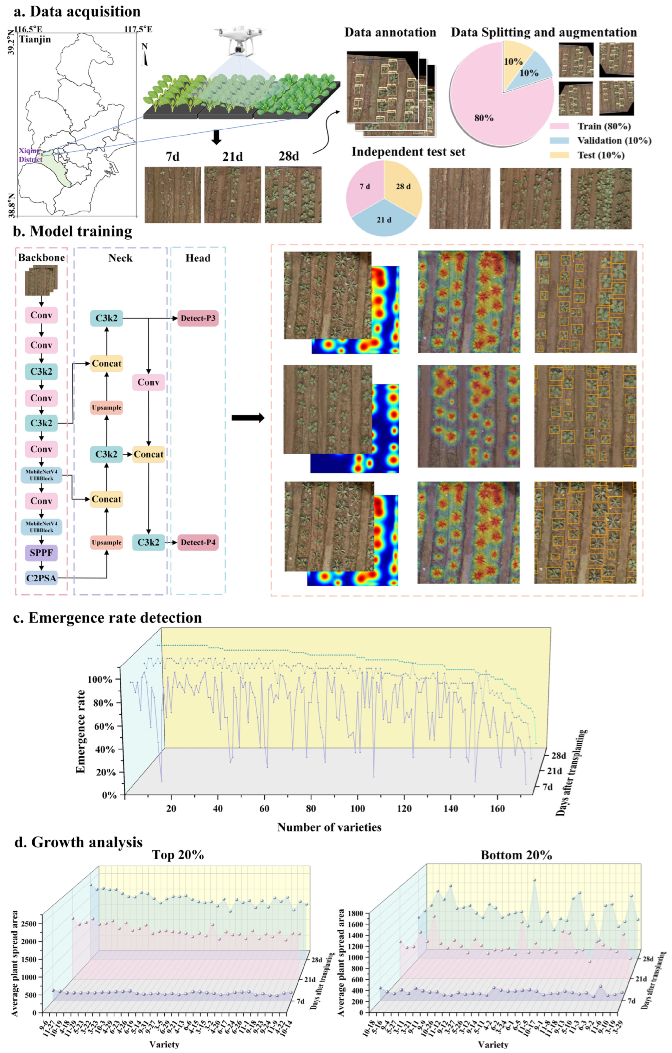
Field experiments were conducted at the experimental site of the Cauliflower Technology Achievement Transformation Base, National Vegetable Industry Technology System, located in Xiqing District, Tianjin, China. A total of 171 cauliflower varieties were planted, and standardized cultivation management practices were adopted to ensure consistent field growth conditions. The experiment was conducted between August and September 2025. UAV imagery was collected at three critical seedling growth stages: 7, 21, and 28 d after transplanting. The workflow of this study is illustrated in Figure 1.

2.2. UAV System and Data Acquisition

The DJI P4M UAV platform (SZ DJI Technology Co., Ltd., Shenzhen, China) was used to acquire field imagery data for cauliflower seedlings. Each flight simultaneously acquired six images, including one RGB image and five grayscale single-band images. Since this study primarily focused on seedling identification, counting, and phenotypic parameter extraction, without involving spectral feature or vegetation index analysis, RGB images with a resolution of 1600 × 1300 pixels were selected for subsequent analysis. Relevant flight and camera parameters are listed in

Table 1. Parameter settings.

Type	Parameters
Flight height	8 m
Heading overlap rates	80%
Side overlap rates	70%
Flight speed	3 m/s
Optimum image size	1600 × 1300 pixels
Sensor width	4.86 mm
Focal length	5.74 mm
GSD	0.423 cm/pixel

. The flight parameters were set to ensure comprehensive image coverage of the study area.

To ensure consistency of the multitemporal data, unified flight route planning was conducted for the experimental area before the first data acquisition. The same flight path and parameters were used for image acquisition at each subsequent time point. Data were collected at three time points (7, 21, and 28 d) after cauliflower seedling transplanting. During image acquisition, a fixed-point hovering mode was adopted to reduce the effects of flight vibration on image quality and improve seedling recognition stability.

Image processing and model construction in this study were performed on a 64-bit Windows 10 operating system, using a hardware platform equipped with an NVIDIA RTX 3090 GPU with 24 GB of memory. Model training was conducted using Python 3.11 and the PyTorch 2.2.1 framework.

2.3. Data Preprocessing

2.3.1. Orthomosaic Generation

In total, 13,344 raw UAV images were imported into DJI Terra 3.9 (DJI Technology Co., Ltd., Shenzhen, China) for orthomosaic stitching to generate digital orthophoto maps (DOMs). ENVI 5.6 (Harris Geospatial Solutions, Inc., Broomfield, CO, USA) was used to crop and preprocess the generated DOMs, remove non-study areas, and retain only the experimental area containing cauliflower seedlings. After processing, seven DOM subregions covering the experimental area were obtained at each time point, and each image had a size of 13,537 × 2217 pixels. A total of 21 high-quality DOMs were obtained for subsequent analyses. In addition, an independent experimental plot with no spatial overlap with the original 21 DOMs was selected, and the DOMs acquired from this plot at 7, 21, and 28 days after transplanting were used as an independent test set.

2.3.2. Image Cropping

Non-target areas were removed from the DOMs acquired at 7, 21, and 28 d after cauliflower seedling transplantation, and the retained field regions were cropped according to a uniform cropping rule to construct the dataset. This ensured that the samples covered the morphological characteristics of seedlings at different growth stages and improved the ability of the model to recognize seedling-stage morphological differences.

To improve the computational efficiency of the model, the original images were cropped using Python, resulting in 931 images of 640 × 640 pixels for model training and evaluation. The independent test set was processed using the same cropping method, resulting in a total of 90 images, with the numbers of images at the three time points in a ratio of 1:1:1. Each cauliflower seedling was annotated using a rectangular bounding box in LabelImg (version 1.8.6), with the box fitted as closely as possible to the visible edges of the plant, and the label was set to “seedling”.

2.3.3. Data Augmentation

The 931 cropped images were randomly divided into training, testing, and validation sets in a ratio of 8:1:1, including 743 images for training, 94 images for testing, and 94 images for validation.

To improve the generalization ability of the model, data augmentation was applied only to the training set, including horizontal flipping, vertical flipping, and diagonal flipping. No data augmentation was applied to either the validation set or the test set, and both were kept in their original form. During the augmentation process, the corresponding label files, including the target class, center coordinates (x and y), width, and height, were updated simultaneously to ensure consistency between the augmented images and their labels. Finally, the number of training samples was increased from 743 to 2972.

2.4. Object Detection Model Construction

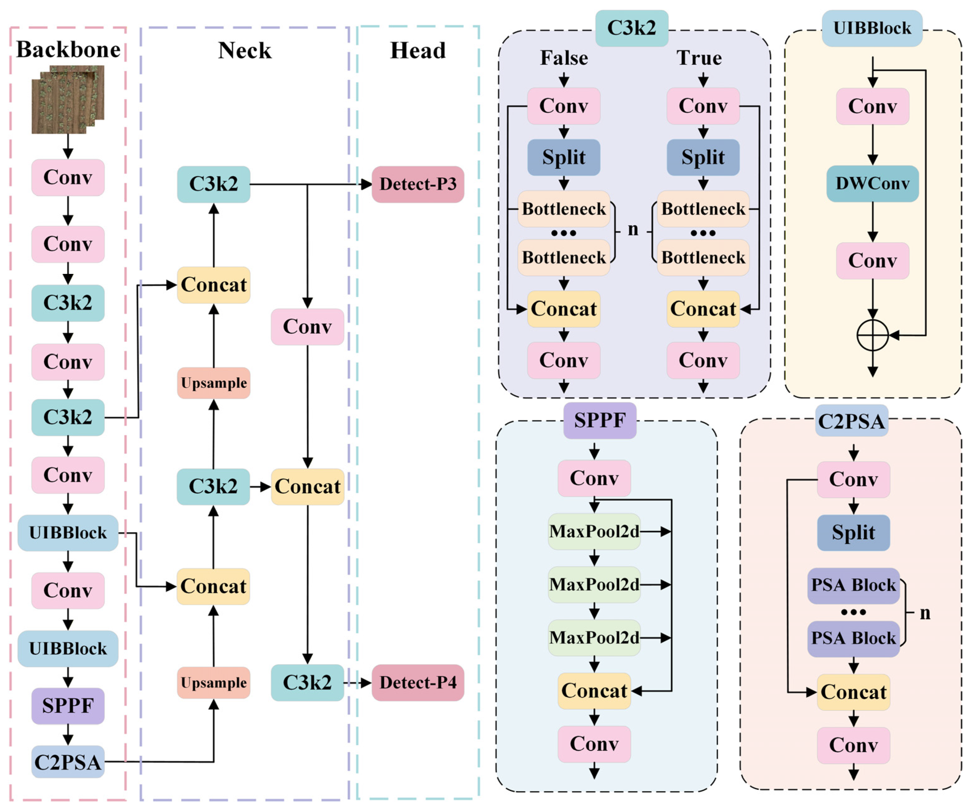
YOLOv11 achieves competitive detection accuracy across various object-detection tasks [33]. To achieve accurate counting of cauliflower seedlings and statistical analysis of growth parameters, YOLOv11 was adopted as the baseline model. Based on this architecture, a lightweight network was designed to develop the DualSlim-YOLO model for cauliflower seedling detection, emergence rate estimation, and growth parameter extraction. The overall network architecture is illustrated in Figure 2.

The main improvements in the YOLOv11 model are as follows:

(1)

Optimization of the Lightweight Feature Extraction Module

In the high-level feature extraction stages (P4/16 and P5/32) of the backbone network, the UIBBlock module from MobileNetV4 was introduced to replace some of the C3k2 feature extraction modules. UIBBlock has a strong lightweight feature representation capability and preserves high-level semantic information while reducing model parameters and computational costs [34], thereby improving detection efficiency for cauliflower seedlings under complex field backgrounds.

(2)

Optimization of the Dual-Scale Detection Head

Owing to the low resolution of the P5 feature map, it is more suitable for detecting large objects, whereas cauliflower seedlings are small targets. Therefore, the P5 detection head in the original YOLOv11 was removed, and the P3/8 and P4/16 detection branches were retained to enhance the model’s ability to detect small- and medium-scale seedling targets while reducing redundant computations, resulting in a dual-scale detection structure tailored for seedling detection tasks.

The deep semantic features from the P5 layer were preserved and fused with the P4 features via upsampling. This design reduces the number of detection branches while retaining high-level semantic information, thereby reducing computational redundancy and maintaining detection performance for small seedling targets.

2.5. Seedling Emergence Rate Estimation and Growth Prediction

2.5.1. Emergence Rate

Based on the DualSlim-YOLO model, UAV-acquired cauliflower seedling images were identified and counted. The emergence rate of each cultivar at all sampling stages was calculated by comparing the model-detected seedling counts with the actual number of transplanted seedlings (Equation (1)).

$$\mathit{ER}={\displaystyle \frac{N_d}{N_t}}\times 100\%$$

(1)

where ER represents the emergence rate, N_d represents the number of seedlings identified by the object detection model, and N_t represents the actual number of transplanted seedlings.

2.5.2. Growth Parameter Extraction

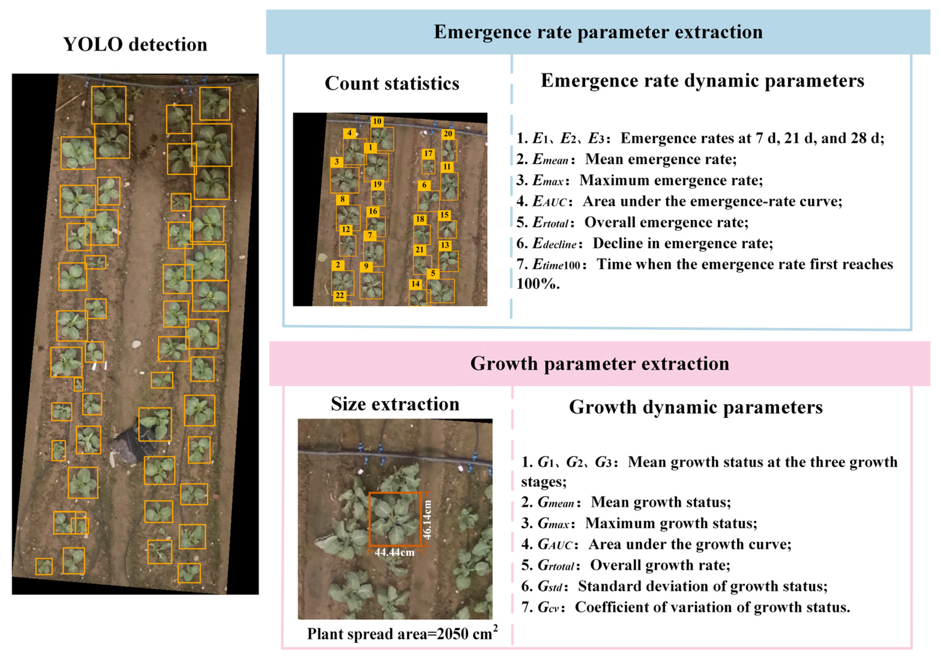
Based on the detection results of DualSlim-YOLO, the target bounding boxes were extracted, and the pixel scale was converted to the actual dimensions using the ground sample distance (GSD) of the UAV images (Equation (2)).

$$\mathit{GSD}={\displaystyle \frac{H\times a}{f}}$$

(2)

where a is the camera pixel pitch, and f is the camera focal length. The pixel pitch a is defined in Equation (3).

$$a={\displaystyle \frac{S_w}{I_w}}$$

(3)

where S_w represents the width of the camera sensor and I_w represents the image width in pixels.

Based on the GSD, the pixel size P in the image can be converted into the actual size D using Equation (4).

$$D=P\times \mathit{GSD}$$

(4)

Using this method, the detected bounding box information was converted into actual spatial dimensions, thereby estimating individual seedling phenotypic parameters, including plant length, plant width, and plant spread area. Plant length was defined as the estimated long side of the bounding box, plant width was defined as the estimated short side of the bounding box, and the plant spread area was calculated as the product of the bounding box length and width.

2.5.3. Construction of Comprehensive Evaluation Indicators

To comprehensively evaluate the seedling growth status of different varieties, we calculated two dynamic phenotypic indicators: emergence rate and growth performance. These indicators were derived from the detection results at 7, 21, and 28 d after seedling transplantation, resulting in a total of 18 features.

The emergence rate indicators included the emergence rate at 7 d (E₁), 21 d (E₂), 28 d (E₃), mean emergence rate (E_mean), maximum emergence rate (E_max), area under the emergence-rate curve (E_AUC), overall emergence rate (E_rtotal), decline in emergence rate (E_decline), and the time when the emergence rate first reached 100% (E_time100), comprising a total of nine dynamic parameters.

Growth indicators were statistically analyzed based on the detection results of the same variety at different time points (7, 21, and 28 d). These indicators included the mean growth status at 7 d (G₁), 21 d (G₂), 28 d (G₃), mean growth status (G_mean), maximum growth status (G_max), area under the growth curve (G_AUC), overall growth rate (G_rtotal), standard deviation of growth status (G_std), and coefficient of variation in growth status (G_cv), comprising a total of nine dynamic parameters. These indicators were used to characterize seedling growth levels and dynamic growth changes of different varieties.

Overall, 18 phenotypic features were used for the subsequent comprehensive evaluation. The extraction workflow is shown in Figure 3, and the corresponding calculation formulae are provided in Appendix A.1 (

Table A1. Growth feature extraction parameters and definitions.

Parameter	Description
E1	E1: Emergence rate at 7 d
E2	E2: Emergence rate at 21 d
E3	E3: Emergence rate at 28 d
$E_{\mathit{mean}}={\displaystyle \frac{E_1+E_2+E_3}{3}}$	$E_{\mathit{mean}}$: Mean emergence rate
$E_{\mathit{max}}=\mathit{max}(E_1,E_2,E_3)$	Emax: Maximum emergence rate
$E_{\mathit{AUC}}={\displaystyle \frac{{\sum }_{i=1}^2(t_{i+1}-t_i)\cdot \frac{E_i+E_{i+1}}{2}}{t_3-t_1}}$	$E_{\mathit{AUC}}$: Area under the emergence-rate curve
$E_{\mathit{rtotal}}={\displaystyle \frac{E_3-E_1}{t_3-t_1}}$	$E_{\mathit{rtotal}}$: Overall emergence rate
$E_{\mathit{decline}}=\mathit{max}(0,E_1-E_2)+\mathit{max}(0,E_2-E_3)$	$E_{\mathit{decline}}$: Decline in emergence rate
$E_{\mathit{time}100}=\left\{\begin{array}{c}{t}_1,E_1\ge 100\\ t_2,E_1<100, E_2\ge 100\\ t_3,E_1<100, E_2<100, E_3\ge 100\\ t_3+\Delta t_{23},E_1<100, E_2<100, E_3<100\end{array}\right.$	$E_{\mathit{time}100}$: Time when the emergence rate first reached 100%
$G_1={\displaystyle \frac{1}{n_1}}\sum A_i^{7d}$($A_i^t=(W_i^t\times \mathit{GSD}\left)\right(H_i^t\times \mathit{GSD})$)	$G_1$: Mean growth status at 7 d
$G_2={\displaystyle \frac{1}{n_2}}\sum A_i^{21d}$	${\mathrm{G}}_2$: Mean growth status at 21 d
$G_3={\displaystyle \frac{1}{n_3}}\sum A_i^{28d}$	$G_3$: Mean growth status at 28 d
$G_{\mathit{mean}}={\displaystyle \frac{G_1+G_2+G_3}{3}}$	$G_{\mathit{mean}}$: Mean growth status
$G_{\max }=\max (G_1,G_2,G_3)$	$G_{\max }$: Maximum growth status
$G_{\mathit{AUC}}={\displaystyle \frac{{{\sum }_{i=1}^2(t}_{i+1}-t_i)\frac{G_i+G_{i+1}}{2}}{t_3-t_1}}$	$G_{\mathit{AUC}}$: Area under the growth curve
$G_{\mathit{rtotal}}={\displaystyle \frac{G_3-G_1}{t_3-t_1}}$	$G_{\mathit{rtotal}}$: Overall growth rate
$G_{\mathit{std}}=\sqrt{{\displaystyle \frac{(G_1-G_{\mathit{mean}}{)}^2+(G_2-G_{\mathit{mean}}{)}^2+(G_3-G_{\mathit{mean}}{)}^2}{2}}}$	$G_{\mathit{std}}$: Standard deviation of growth status
$G_{\mathit{cv}}={\displaystyle \frac{G_{\mathit{std}}}{G_{\mathit{mean}}+\mathsf{ϵ}}}$	$G_{\mathit{cv}}$: Coefficient of variation of growth status, $ϵ$: Infinitesimal constant

Note: t_i denotes the time point (i = 1, 2, 3); $A_i^t$ denotes the area of the ith plant at time t; $W_i^t$ denotes the width of the detection box; $H_i^t$ denotes the height of the detection box; and $n_t$ denotes the number of samples at the corresponding time point.

).

To eliminate the effects of differences in indicator dimensions and directions on the comprehensive evaluation results, each indicator was first unified in direction and normalized using range standardization. For the positive indicators, Equation (5) was used for normalization, whereas Equation (6) was used for the reverse normalization of negative indicators, therefore all indicators were transformed such that larger values indicated better performance.

$$Z_{\mathit{ij}}={\displaystyle \frac{X_{\mathit{ij}}-X_{j,\min }}{X_{j,\max }-X_{j,\min }}}$$

(5)

$$Z_{\mathit{ij}}={\displaystyle \frac{X_{j,\max }-X_{\mathit{ij}}}{X_{j,\max }-X_{j,\min }}}$$

(6)

$X_{\mathit{ij}}$ represents the original value of the ith variety for the jth evaluation indicator, $X_{j,\mathit{min}}$ and $X_{j,\mathit{max}}$ represent the minimum and maximum values of the jth evaluation indicator among all varieties, respectively, and $Z_{\mathit{ij}}$ represents the standardized indicator value.

To reduce information redundancy among the different indicators, principal component analysis (PCA) was performed on the standardized evaluation indicators, and the resulting principal components (PCs) were extracted as comprehensive variables (F₁, F₂, F₃, …, F_i).

Based on the dimensionality reduction results, min-max normalization was performed on the scores of each PC to obtain the corresponding membership function values (Equation (7)). The weight of each PC is determined based on the proportion of the variance contribution rate to the cumulative contribution rate of the selected PCs (Equation (8)). Finally, the comprehensive evaluation D value was obtained by weighting and summing the membership function values of all PCs (Equation (9)):

$$\mu (X_i)={\displaystyle \frac{F_i-F_{\mathit{min}}}{F_{\mathit{max}}-F_{\mathit{min}}}}$$

(7)

$$w_i={\displaystyle \frac{p_i}{{\displaystyle {\sum }_{i=1}^n}{p}_i}}$$

(8)

$$\begin{array}{c}D={\displaystyle \sum _{i=1}^n}\left[\mu \left(X_i\right)\times w_i\right]\end{array}$$

(9)

where F_i represents the ith PC; F_min and F_max represent the minimum and maximum values of the ith PC, respectively; w_i represents the weight of the ith PC; and p_i represents the contribution rate of the ith PC.

To quantify the relationships between the phenotypic traits and the comprehensive seedling growth indicator D, stepwise regression was used for variable selection. The criteria for variable entry and removal were set at p < 0.05 and p > 0.10, respectively, and a multiple linear regression (MLR) model, S, was further constructed for rapid quantitative evaluation of seedling growth performance.

$$\begin{array}{c}S={\beta }_0+{\sum }_{j=1}^m{\beta }_j{X}_j\end{array}$$

(10)

β₀ is the regression intercept, β_j is the regression coefficient corresponding to the jth feature variable, X_j represents the jth feature variable, and m represents the number of feature variables included in the model.

2.6. Evaluation Metrics

2.6.1. Model Evaluation Metrics

To evaluate the detection performance of DualSlim-YOLO, Precision (P), Recall (R), F1-score, mean Average Precision at an Intersection over Union (IoU) threshold of 0.5 (mAP@0.5), and mean Average Precision averaged over IoU thresholds from 0.5 to 0.95 in steps of 0.05 (mAP@0.5:0.95) were used as evaluation metrics (Equations (11)–(17)), thereby providing a comprehensive assessment of the object-detection algorithm.

$$P={\displaystyle \frac{\mathit{TP}}{\mathit{TP}+\mathit{FP}}}$$

(11)

where TP represents true positives, namely correctly predicted target instances, and FP represents false positives, namely incorrectly predicted target instances.

$$R={\displaystyle \frac{\mathit{TP}}{\mathit{TP}+\mathit{FN}}}$$

(12)

where FN represents false negatives, namely target instances that were not detected.

$$F1-\mathit{Score}={\displaystyle \frac{2\times \mathit{Precision}\times \mathit{Recall}}{\mathit{Precision}+\mathit{Recall}}}$$

(13)

$$\begin{array}{c}AP={\int }_0^{1}P\left(R\right)dR\end{array}$$

(14)

$$\begin{array}{c}mAP={\displaystyle \frac{1}{n}}{\displaystyle \sum _{i=1}^n}A{P}_i\end{array}$$

(15)

$$\begin{array}{c}mA{P}_{0.5}={\displaystyle \frac{1}{n}}{\sum }_{i=1}^{n}A{P}_i^{0.5}\times 100\%,\hspace{1em}IoU\ge 0.5\end{array}$$

(16)

where n represents the total number of classes in the dataset, AP_i represents the average precision of the ith class, and $A{P}_i^{0.5}$ represents the average precision of the ith class at an IoU threshold of 0.5.

$$\begin{array}{c}mA{P}_{0.5:0.95}={\displaystyle \frac{1}{10}}{\sum }_{k=0}^{9}mA{P}_{0.50+0.05k}\end{array}$$

(17)

where k represents the index of the IoU threshold.

2.6.2. Evaluation Metrics for Counting and Emergence Rate Estimation

To evaluate the accuracy of the model in practical seedling counting and emergence rate estimation, counting mean absolute error (Counting MAE, MAE_count), counting root mean square error (Counting RMSE, RMSE_count), and emergence-rate mean absolute error (Emergence-rate MAE, MAE_ER) were used as evaluation metrics (Equations (18)–(20)).

$$\begin{array}{c}MA{E}_{\mathit{count}}={\displaystyle \frac{1}{n}}{\sum }_{i=1}^n\left|{\widehat{N}}_i-N_i\right|\end{array}$$

(18)

$$\begin{array}{c}RMS{E}_{\mathit{count}}=\sqrt{{\displaystyle \frac{1}{n}}{\sum }_{i=1}^n{\left({\widehat{N}}_i-N_i\right)}^2}\end{array}$$

(19)

$$\begin{array}{c}MA{E}_{\mathit{ER}}={\displaystyle \frac{1}{n}}{\sum }_{i=1}^n\left|{\widehat{\mathit{ER}}}_i-E{R}_i\right|\end{array}$$

(20)

where ${\widehat{N}}_i$ and $N_i$ represent the number of seedlings of the ith variety obtained from model prediction and manual counting, respectively; ${\widehat{\mathit{ER}}}_i$ and $E{R}_i$ represent the emergence rates of the ith variety calculated based on model prediction and manual counting, respectively; and n denotes the number of varieties included in the evaluation.

3. Results

3.1. Seedling Detection Results

3.1.1. Comparison of Different Seedling Recognition Algorithms

To select an object detection model suitable for seedling-stage recognition and feature extraction, Faster R-CNN, YOLOv8, YOLOv11, and YOLOv12 were selected for comparative experiments in this study. To ensure the comparability of the experimental results, all models were trained and tested under the same environment and parameter settings, and the results are listed in

Table 2. Comparison of the performance of different seedling detection models.

Model	P (%)	R (%)	F1-Score (%)	mAP@0.5 (%)	mAP@0.5:0.95 (%)
Faster R-CNN	75.27	98.18	85.21	96.52	65.23
YOLOv8	94.90	95.60	95.25	97.50	85.70
YOLOv11	94.92	96.60	95.75	98.16	86.55
YOLOv12	95.32	95.25	95.28	98.28	86.25

. Compared with YOLOv12, YOLOv11 achieved better performance in terms of Recall, F1-score, and mAP@0.5:0.95. Considering that missed detections may affect subsequent seedling counting and emergence rate estimation, YOLOv11 was selected as the baseline model for subsequent model improvements.

3.1.2. Model Improvement and Comparison

To meet the requirements for real-time detection of small cauliflower seedlings in complex field scenarios, this study used YOLOv11 as the baseline model to investigate lightweight and feature-enhancement improvements. The effects of different lightweight modules and feature fusion strategies on the model performance were compared through multiple ablation experiments, and the optimal network architecture suitable for cauliflower seedling detection was selected. Different improvement strategies showed differences in detection accuracy, model complexity, and inference speed, and the results are listed in

Table 3. Performance comparison of cauliflower seedling detection models under different improvement strategies.

Model	P (%)	R (%)	F1-Score (%)	mAP@0.5 (%)	mAP@0.5:0.95 (%)	Parameters (M)	GFLOPs	FPS
YOLOv11	94.92	96.60	95.75	98.16	86.55	2.59	6.44	56.18
YOLOv11 + P2	95.82	95.15	95.49	98.24	86.06	2.67	10.40	52.51
YOLOv11 + DWRSeg	95.26	96.69	95.97	98.49	86.84	2.61	6.49	53.37
YOLOv11 + DWRSeg + ECA	96.59	95.28	95.93	98.26	86.24	2.61	6.50	52.21
DualSlim-YOLO	95.35	96.75	96.05	98.55	86.65	1.59	5.51	68.63
DualSlim-YOLO + Gate	95.25	96.51	95.88	98.29	86.37	1.64	6.10	67.79

Note: P2 represents the small-object detection layer, DWRSeg represents the convolutional feature enhancement module, ECA represents the efficient channel attention mechanism, and Gate represents the gating mechanism.

. The results showed that DualSlim-YOLO reduced the number of model parameters and computational complexity while maintaining high detection accuracy. Its F1-score and mAP@0.5 reached 96.05% and 98.55%, respectively, which were higher than those of the other models. The model had 1.59 M parameters, a computational cost of 5.51 giga floating-point operations (GFLOPs), and an inference speed of 68.63 frames per second (FPS), indicating better overall performance than the other models. Considering its detection accuracy, model complexity, and inference efficiency, DualSlim-YOLO was selected as the final cauliflower-seedling detection model.

3.1.3. Validation of Model Generalization

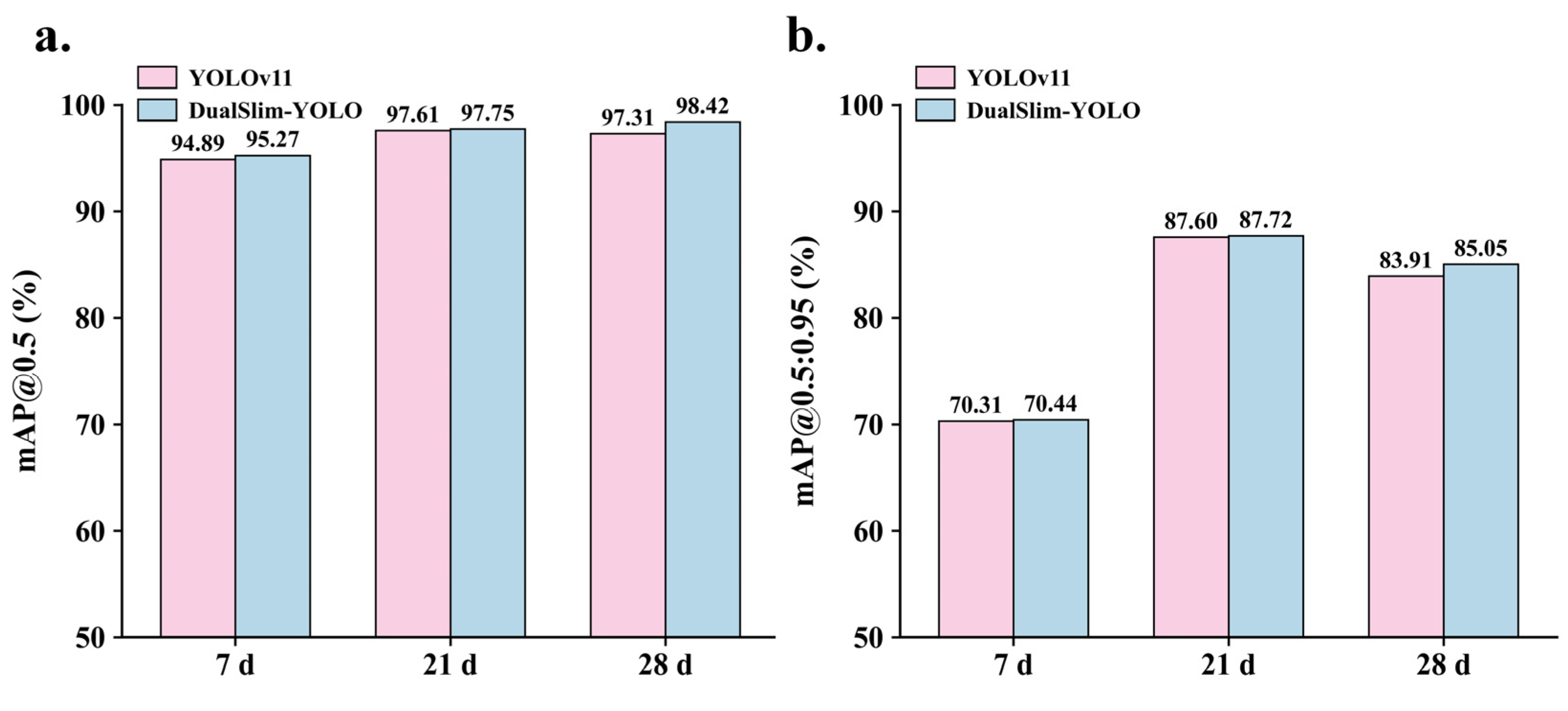
To further evaluate the generalization ability of the model, the independent test set was used as external validation data. This test set was not involved in model training, validation, or model selection. To ensure the comparability of the evaluation results, all tests were conducted using fixed model weights and inference parameters. The overall detection performance of the model was evaluated using all images in the independent test set (

Table 4. Overall performance on the independent test set.

Model	P (%)	R (%)	F1-Score (%)	mAP@0.5 (%)	mAP@0.5:0.95 (%)	Parameters (M)	GFLOPs	FPS
YOLOv11	96.27	95.15	95.70	96.71	81.65	2.59	6.44	56.32
DualSlim-YOLO	95.58	96.50	96.04	97.25	82.02	1.59	5.51	64.02

). The images acquired at 7, 21, and 28 days after transplanting were then evaluated separately to analyze the detection performance of the model at different time points (Figure 4).

The results showed that DualSlim-YOLO achieved good overall performance in terms of Recall, F1-score, mAP@0.5, and mAP@0.5:0.95, while reducing the number of model parameters and computational complexity and improving inference speed. In the evaluations at different time points, its mAP@0.5 and mAP@0.5:0.95 were consistently higher than those of YOLOv11. These results indicate that the model achieves a good balance between detection performance and inference efficiency while demonstrating good generalization ability on the external cauliflower test plot.

3.1.4. Ablation Experiments

To verify the effectiveness of the improvement strategies in DualSlim-YOLO, ablation experiments were conducted on the same dataset used in this study, and the results are shown in

Table 5. Results of the ablation study.

Model	P4/16 UIBBlock	P5/32 UIBBlock	P5 Detect Removed	P (%)	R (%)	F1-Score (%)	mAP@0.5 (%)	mAP@0.5:0.95 (%)	Parameters (M)	GFLOPs	FPS
YOLOv11	-	-	-	94.92	96.60	95.75	98.16	86.55	2.59	6.44	56.18
1	-	-	√	95.84	96.03	95.93	98.33	86.63	1.85	5.85	68.36
2	√	-	-	94.85	96.63	95.74	98.40	86.58	2.54	6.27	59.04
3	-	√	-	94.88	96.45	95.66	98.44	86.59	2.38	6.27	58.61
4	√	√	-	96.29	95.17	95.72	98.42	86.27	2.33	6.10	59.51
5	√	-	√	96.11	95.79	95.95	98.48	86.38	1.80	5.68	66.58
6	-	√	√	95.70	96.21	95.96	98.22	86.32	1.64	5.68	64.15
DualSlim-YOLO	√	√	√	95.35	96.75	96.05	98.55	86.65	1.59	5.51	68.63

Note: “√” indicates that the module was included, while “-” indicates that it was not included.

. Compared with the baseline YOLOv11 model, removing the P5 detection head reduced the number of parameters from 2.59 M to 1.85 M and the number of GFLOPs from 6.44 to 5.85. Meanwhile, the F1-score and mAP@0.5:0.95 increased to 95.93% and 86.63%, respectively, indicating that removing the P5 detection head reduced model complexity while maintaining good detection performance. On this basis, the UIBBlock module from the lightweight MobileNetV4 was further introduced into the high-level feature extraction stage to reduce redundant computations in the backbone network. The resulting DualSlim-YOLO achieved a good balance among detection accuracy, model complexity, and inference speed. Its P, R, F1-score, mAP@0.5, and mAP@0.5:0.95 reached 95.35%, 96.75%, 96.05%, 98.55%, and 86.65%, respectively. The number of parameters and the number of GFLOPs were reduced to 1.59 M and 5.51, respectively, and the inference speed increased to 68.63 FPS.

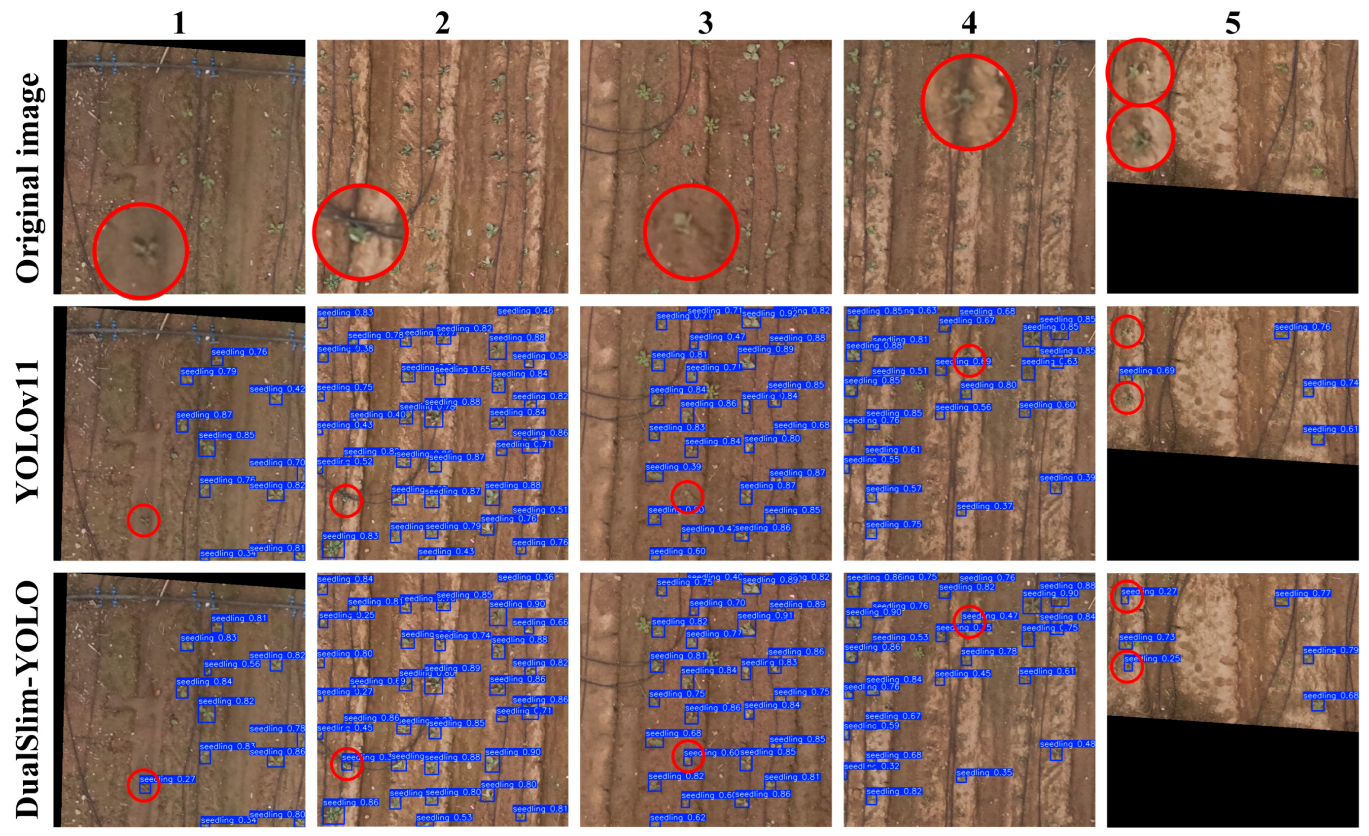
To more clearly demonstrate the effectiveness of the improved model, the detection results of YOLOv11 and DualSlim-YOLO were visually compared, as shown in Figure 5. Compared with the baseline model, DualSlim-YOLO reduced missed and false detections of cauliflower seedlings while maintaining a lightweight architecture.

3.2. Evaluation of Counting Performance

To evaluate the performance of the model in practical seedling counting and emergence rate estimation, 20 cauliflower varieties were selected, and MAE_count, RMSE_count, MAE_ER, and their 95% confidence intervals were calculated at different time points. The results are shown in

Table 6. Counting and Emergence-Rate Estimation Errors at Different Time Points.

Model	Time Point	MAEcount, (Plants 95% CI)	RMSEcount (Plants 95% CI)	MAEER (pp 95% CI)
YOLOv11	7 d	3.75 (2.10–5.65)	5.50 (3.41–7.38)	17.97 (10.13–26.54)
DualSlim-YOLO	7 d	2.80 (1.45–4.40)	4.40 (2.47–6.17)	13.08 (6.59–20.32)
YOLOv11	21 d	0.15 (0.00–0.40)	0.50 (0.00–0.84)	0.68 (0.00–1.80)
DualSlim-YOLO	21 d	0.10 (0.00–0.25)	0.32 (0.00–0.50)	0.47 (0.00–1.18)
YOLOv11	28 d	0.30 (0.10–0.55)	0.63 (0.32–0.92)	1.30 (0.29–2.50)
DualSlim-YOLO	28 d	0.25 (0.05–0.50)	0.59 (0.22–0.89)	1.14 (0.20–2.30)

. DualSlim-YOLO exhibited lower counting errors and emergence rate estimation errors than YOLOv11 at 7, 21, and 28 days. At 7 days, the MAE_count, RMSE_count and MAE_ER of DualSlim-YOLO were 2.80 seedlings, 4.40 seedlings, and 13.08 percentage points, respectively. Compared with the baseline model, these values were reduced by 0.95 seedlings, 1.10 seedlings, and 4.89 percentage points, respectively. The results showed that DualSlim-YOLO achieved good performance in seedling counting and emergence rate estimation at different time points.

3.3. Analysis of Emergence Rates Among Different Varieties

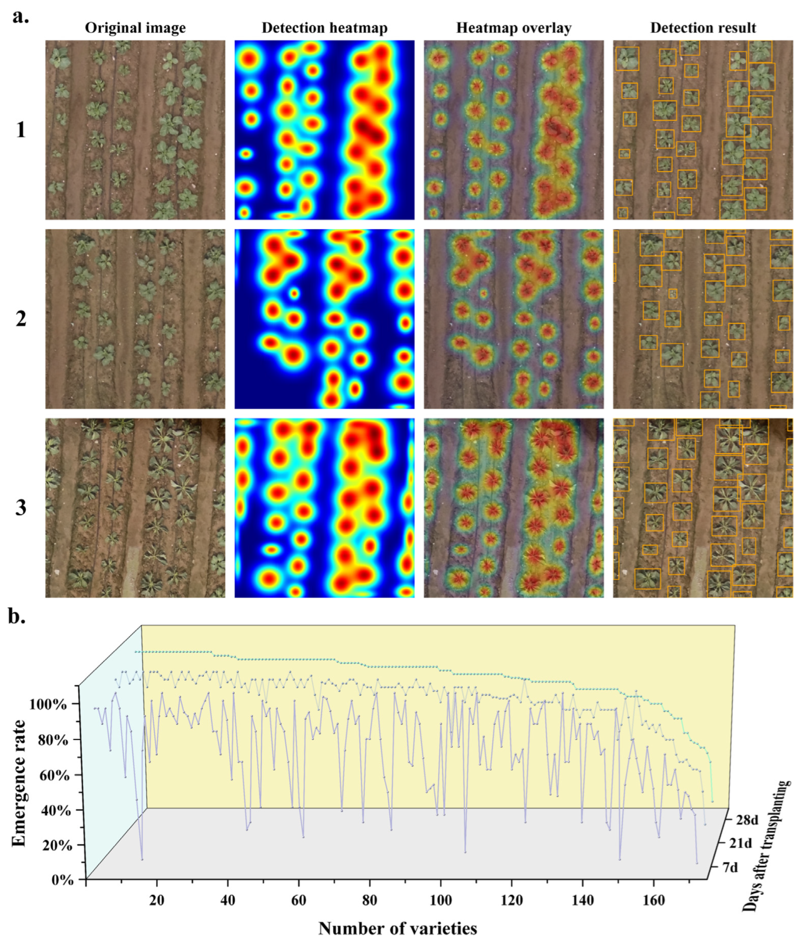
In this study, a lightweight DualSlim-YOLO detection model was used to automatically identify cauliflower seedlings in images acquired 7, 21, and 28 d after transplantation. The feature response regions of the model were visualized using heat maps, as shown in Figure 6a. The high-response areas in the heat maps were mainly concentrated around the seedling canopy and its edges, indicating that the model could accurately capture the characteristics of cauliflower seedlings in the field. Based on this, the emergence rate of each variety at 7, 21, and 28 d was calculated by combining the number of seedlings detected by the model with the number of seedlings transplanted into the field. The varieties were then ranked in descending order according to the final emergence rate at 28 d, as shown in Figure 6b. The ranking results and corresponding variety codes are provided in Appendix A.2 (

Table A2. Ranking results for different cultivars and their corresponding codes.

Variety	E1	E2	E3	Rank	Variety	E1	E2	E3	Rank
5-14	91.30	95.65	100.00	1	9-18	82.61	95.65	91.30	87
4-26	91.30	91.30	100.00	2	9-27	95.65	91.30	91.30	88
11-25	82.61	100.00	100.00	3	3-17	60.87	91.30	91.30	89
9-25	91.30	100.00	100.00	4	9-17	58.70	86.96	89.13	90
9-28	67.39	93.48	100.00	5	9-6	89.13	93.48	89.13	91
6-24	95.65	95.65	100.00	6	4-21	82.61	89.13	89.13	92
11-9	100.00	100.00	100.00	7	9-12	63.04	89.13	89.13	93
4-20	91.30	95.65	100.00	8	6-7	43.48	82.61	86.96	94
9-30	52.17	100.00	100.00	9	9-5	45.65	91.30	86.96	95
5-35	86.96	91.30	100.00	10	9-4	47.83	86.96	86.96	96
11-1	78.26	100.00	100.00	11	9-13	30.43	65.22	86.96	97
9-22	39.13	100.00	100.00	12	5-33	82.61	91.30	86.96	98
6-2	4.35	100.00	100.00	13	9-9	30.43	91.30	86.96	99
10-5	67.39	97.83	100.00	14	4-29	100.00	91.30	86.96	100
4-28	86.96	95.65	100.00	15	4-24	69.57	82.61	86.96	101
10-22	60.87	95.65	100.00	16	4-13	100.00	91.30	86.96	102
9-21	95.65	100.00	100.00	17	4-1	69.57	86.96	86.96	103
10-20	65.22	91.30	100.00	18	3-4	95.65	91.30	86.96	104
4-30	86.96	95.65	100.00	19	10-17	8.70	82.61	86.96	105
3-15	100.00	100.00	100.00	20	4-22	91.30	86.96	86.96	106
5-23	86.96	95.65	100.00	21	3-14	82.61	86.96	86.96	107
3-23	91.30	100.00	100.00	22	10-19	100.00	86.96	86.96	108
4-10	86.96	95.65	100.00	23	3-25	59.42	85.51	85.51	109
10-7	82.61	93.48	97.83	24	4-6	75.36	85.51	85.51	110
3-5	97.83	97.83	97.83	25	11-12	56.52	84.78	84.78	111
9-31	89.13	97.83	97.83	26	11-23	56.52	84.78	84.78	112
6-6	86.96	100.00	97.83	27	6-32	82.61	84.78	84.78	113
6-9	80.43	95.65	97.83	28	6-26	89.57	86.09	84.35	114
6-29	88.41	100.00	97.10	29	9-19	69.57	86.96	84.06	115
5-6	82.61	100.00	97.10	30	10-13	89.86	85.51	84.06	116
4-11	91.30	91.30	95.65	31	3-7	95.65	82.61	82.61	117
5-30	95.65	100.00	95.65	32	3-16	56.52	95.65	82.61	118
5-21	100.00	94.20	95.65	33	11-24	65.22	85.87	82.61	119
5-3	78.26	95.65	95.65	34	6-4	60.87	82.61	82.61	120
6-8	78.26	91.30	95.65	35	10-8	68.12	81.16	82.61	121
3-3	65.22	100.00	95.65	36	9-1	26.09	82.61	82.61	122
4-5	95.65	91.30	95.65	37	4-15	91.30	82.61	82.61	123
4-4	84.78	93.48	95.65	38	4-27	82.61	82.61	82.61	124
5-32	50.72	88.41	95.65	39	4-8	82.61	82.61	82.61	125
6-19	100.00	95.65	95.65	40	5-28	91.30	82.61	82.61	126
5-34	60.87	95.65	95.65	41	4-9	95.65	86.96	82.61	127
5-36	60.87	86.96	95.65	42	9-8	65.22	82.61	82.61	128
9-14	21.74	95.65	95.65	43	4-25	42.24	78.88	81.37	129
6-1	26.09	82.61	95.65	44	9-34	65.22	78.26	78.26	130
6-17	86.96	95.65	95.65	45	10-26	41.30	78.26	78.26	131
3-9	78.26	95.65	95.65	46	3-13	100.00	86.96	78.26	132
5-16	34.78	91.30	95.65	47	10-18	60.87	78.26	78.26	133
3-22	95.65	95.65	95.65	48	5-19	60.87	73.91	78.26	134
9-15	86.96	91.30	95.65	49	4-3	91.30	78.26	78.26	135
9-26	91.30	95.65	95.65	50	10-12	73.91	78.26	78.26	136
9-7	56.52	100.00	95.65	51	4-17	82.61	78.26	78.26	137
10-23	91.30	95.65	95.65	52	6-5	26.09	73.91	78.26	138
11-10	82.61	91.30	95.65	53	4-14	82.61	82.61	78.26	139
11-20	78.26	95.65	95.65	54	4-12	82.61	78.26	78.26	140
3-18	60.87	91.30	95.65	55	3-8	73.91	78.26	78.26	141
11-21	34.78	95.65	95.65	56	6-28	78.26	78.26	78.26	142
11-27	95.65	97.83	95.65	57	11-7	65.22	78.26	76.09	143
11-3	34.78	86.96	95.65	58	3-26	68.12	78.26	75.36	144
11-5	17.39	78.26	95.65	59	9-10	26.09	60.87	73.91	145
10-11	85.51	94.20	94.20	60	5-10	21.74	69.57	73.91	146
9-23	89.13	93.48	93.48	61	6-21	91.30	84.78	73.91	147
9-24	73.91	95.65	93.48	62	6-30	78.26	73.91	73.91	148
9-16	80.43	93.48	93.48	63	11-6	4.35	60.87	73.91	149
9-38	77.17	92.39	93.48	64	3-11	47.83	89.13	71.74	150
6-20	97.83	89.13	93.48	65	6-27	63.04	80.43	71.74	151
11-29	96.74	93.48	93.48	66	5-26	73.91	69.57	69.57	152
10-3	89.86	93.48	92.75	67	9-3	63.04	71.74	69.57	153
5-25	77.39	95.65	92.17	68	3-27	54.35	67.39	69.57	154
10-16	82.61	95.65	91.30	69	4-2	43.48	69.57	69.57	155
9-37	32.61	93.48	91.30	70	3-28	69.57	65.22	65.22	156
10-21	67.39	86.96	91.30	71	11-19	56.52	69.57	65.22	157
6-31	85.51	92.75	91.30	72	5-27	45.65	63.04	63.04	158
5-29	95.65	91.30	91.30	73	9-2	26.09	60.87	60.87	159
4-23	82.61	91.30	91.30	74	6-3	17.39	60.87	60.87	160
10-14	86.96	86.96	91.30	75	3-6	65.22	60.87	60.87	161
5-11	26.09	95.65	91.30	76	5-24	47.83	52.17	52.17	162
5-13	73.91	91.30	91.30	77	5-12	47.83	47.83	52.17	163
5-1	73.91	91.30	91.30	78	3-20	56.52	47.83	47.83	164
4-18	91.30	91.30	91.30	79	3-21	44.93	49.28	46.38	165
9-33	100.00	91.30	91.30	80	11-18	28.26	45.65	45.65	166
4-16	73.91	91.30	91.30	81	11-8	43.48	43.48	43.48	167
11-2	52.17	93.48	91.30	82	3-10	41.30	43.48	43.48	168
3-12	43.48	91.30	91.30	83	3-24	33.70	42.39	40.22	169
9-11	21.74	86.96	91.30	84	3-19	30.43	30.43	34.78	170
6-23	100.00	91.30	91.30	85	3-29	2.17	10.87	10.87	171
3-2	89.13	91.30	91.30	86

). The results showed that the emergence rates of different varieties varied markedly across the three time points. Seven days after transplantation, the emergence rates varied considerably among the varieties, indicating clear differences in emergence speed. At 21 d, the overall emergence rate increased substantially. By 28 d, most varieties had reached an emergence rate of 100%, whereas a few varieties still showed relatively low emergence rates, indicating differences in seedling establishment ability among the varieties.

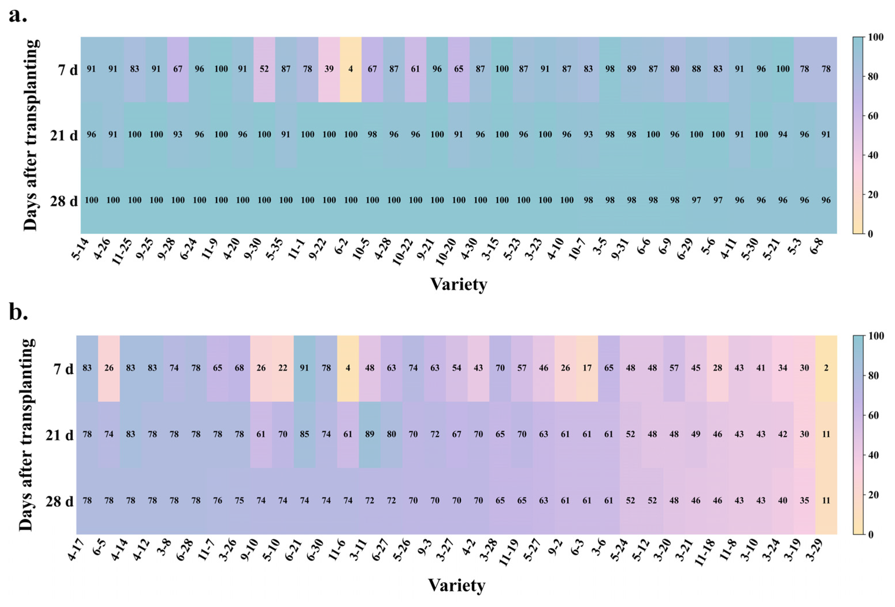
To further analyze the dynamic characteristics of emergence rates, the 171 varieties were grouped into the top 20% and bottom 20% according to the overall distribution of emergence rates (171 × 0.2 = 34.2, rounded up to 35 varieties per group), and heat maps of emergence rates at the three time points were plotted separately (Figure 7). The results showed that the top 20% of varieties had the highest overall emergence rates. By 21 d, most of these varieties had reached emergence rates of 90–100% and maintained these rates at 28 d, indicating good emergence ability. In contrast, the bottom 20% of the varieties showed relatively low final emergence rates with large differences among them. Some varieties showed no improvement at 28 d, indicating slow emergence speed and poor final seedling establishment ability.

3.4. Comprehensive Evaluation of Dynamic Seedling-Stage Characteristics

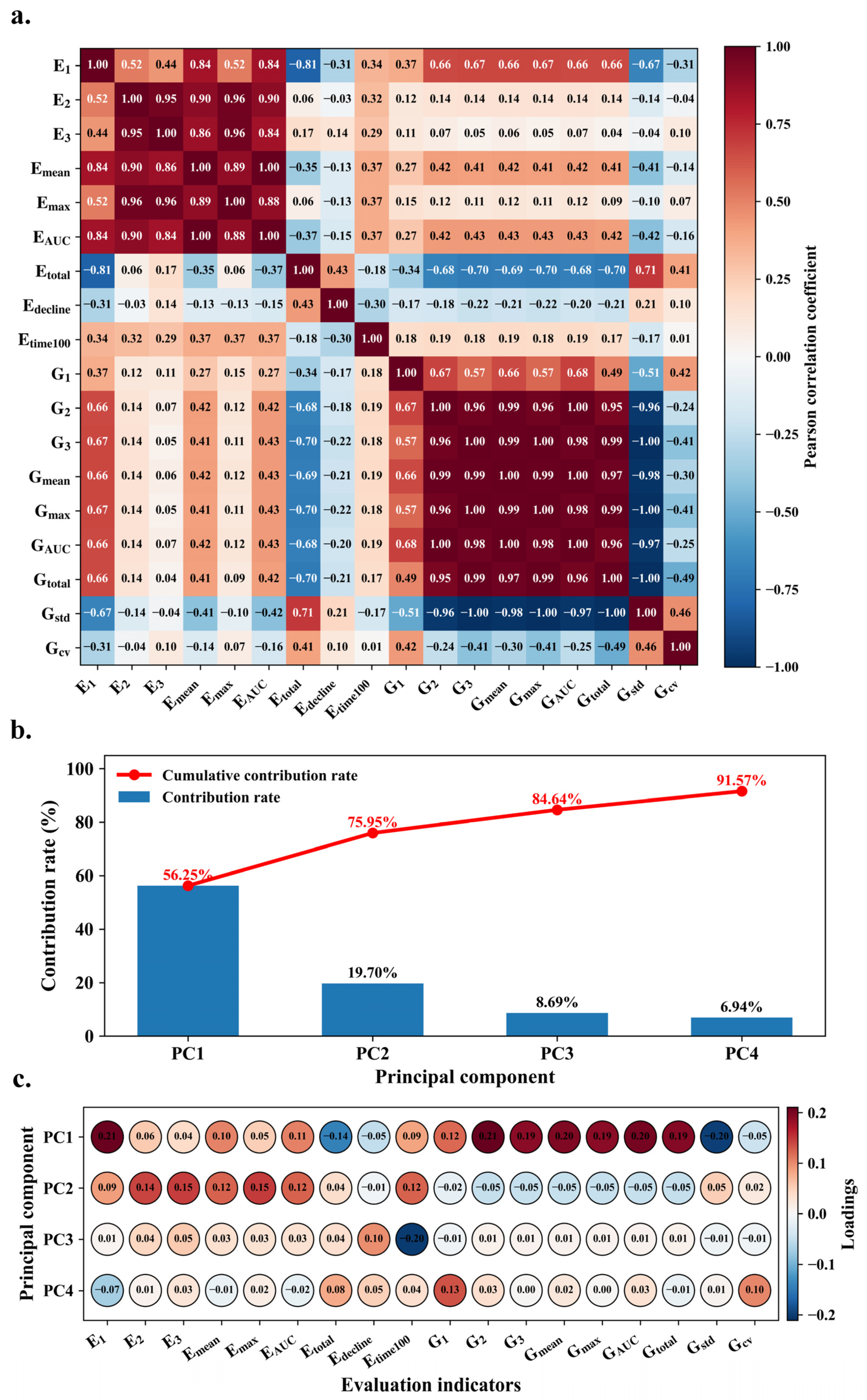
Based on the detection results of the DualSlim-YOLO model, field emergence rates and bounding box information were used to extract nine dynamic emergence rate parameters and nine dynamic growth parameters. Eighteen dynamic seedling-stage features were obtained. To eliminate the effects of differences in indicator dimensions and directions on the comprehensive evaluation results, each indicator was first adjusted to a common direction and standardized using range normalization. To reveal the correlations and potential information redundancies among different dynamic characteristics, a correlation heatmap was generated (Figure 8a), which showed strong correlations between emergence rate indicators and growth indicators. Therefore, principal component analysis (PCA) was applied to the 18 dynamic features, and the first four principal components (PCs) were extracted, explaining 91.57% of the cumulative variance (Figure 8b).

The contribution of each original variable to the PCs was analyzed using a PCA loading plot (Figure 8c). The results showed that PC1 had high loading values for E₁, multiple growth indicators, and cumulative growth indicators, reflecting the early emergence and growth advantage of the seedling population. PC2 was primarily influenced by emergence-related indicators, representing the overall emergence ability and process of the varieties. PC3 and PC4 focused on emergence dynamics, early-growth performance, and growth fluctuation parameters, reflecting differences in seedling-stage dynamic changes and stability among varieties.

These results indicate that each PC represents seedling-stage phenotypes from three dimensions: emergence ability, growth level, and stability. These dimensions correspond well to the multidimensional evaluation system used for the comprehensive evaluation based on the D value.

Based on the PCA dimensionality reduction results, the D value for each variety was calculated by integrating the scores of each PC with the corresponding contribution-rate weights. To facilitate comparison among different varieties, the D values were further normalized and mapped to a 0–100 range, which was used as the comprehensive evaluation score for the seedling growth performance of different varieties.

3.5. Construction of the Comprehensive Growth Evaluation Model and Variety Screening

3.5.1. Construction of an MLR-Based Comprehensive Model

To construct an interpretable quantitative evaluation model for seedling growth performance, the comprehensive evaluation indicator D was used as the dependent variable. Based on the results of stepwise variable selection, E_decline and G_cv were excluded, and the remaining variables were used to construct the multiple linear regression (MLR) model S (Equation (21)). This model can directly use the original feature parameters extracted in batches from UAV-based detection and rapidly output a comprehensive seedling growth score for each variety, making it suitable for subsequent large-scale quantitative assessments of field seedling conditions.

S = −25.9941 + 0.0782 × E₁ + 0.0714 × E₂ + 0.2001 × E₃ + 0.1484 × E_mean − 0.0024 × E_max + 0.1269 × E_AUC − 0.1471 × E_rtotal − 0.0846 × E_time100 + 0.0352 × G₁ + 0.0065 × G₂ + 0.0044 × G₃ + 0.0079 × G_mean + 0.0044 × G_max + 0.0086 × G_AUC + 0.0941 × G_rtotal − 0.0041 × G_std

(21)

3.5.2. Growth Indicator Selection and Validation of Comprehensive Evaluation Results

The regression coefficients in the comprehensive model S are affected by feature scales and, therefore, cannot be directly used to evaluate variable contributions. Among all canopy growth-related indicators (G₁, G₂, G₃, G_mean, G_max, G_AUC, G_rtotal, and G_std), G_AUC and G_rtotal represent the cumulative seedling growth level and overall growth rate, respectively, and can effectively reflect the dynamic changes in seedling growth performance. Emergence indicators such as E₁, E₂, and E₃ reflect only the number of seedlings and do not represent overall seedling growth performance. Therefore, G_AUC and G_rtotal were selected as representative growth indicators to validate the discriminative performance of the model.

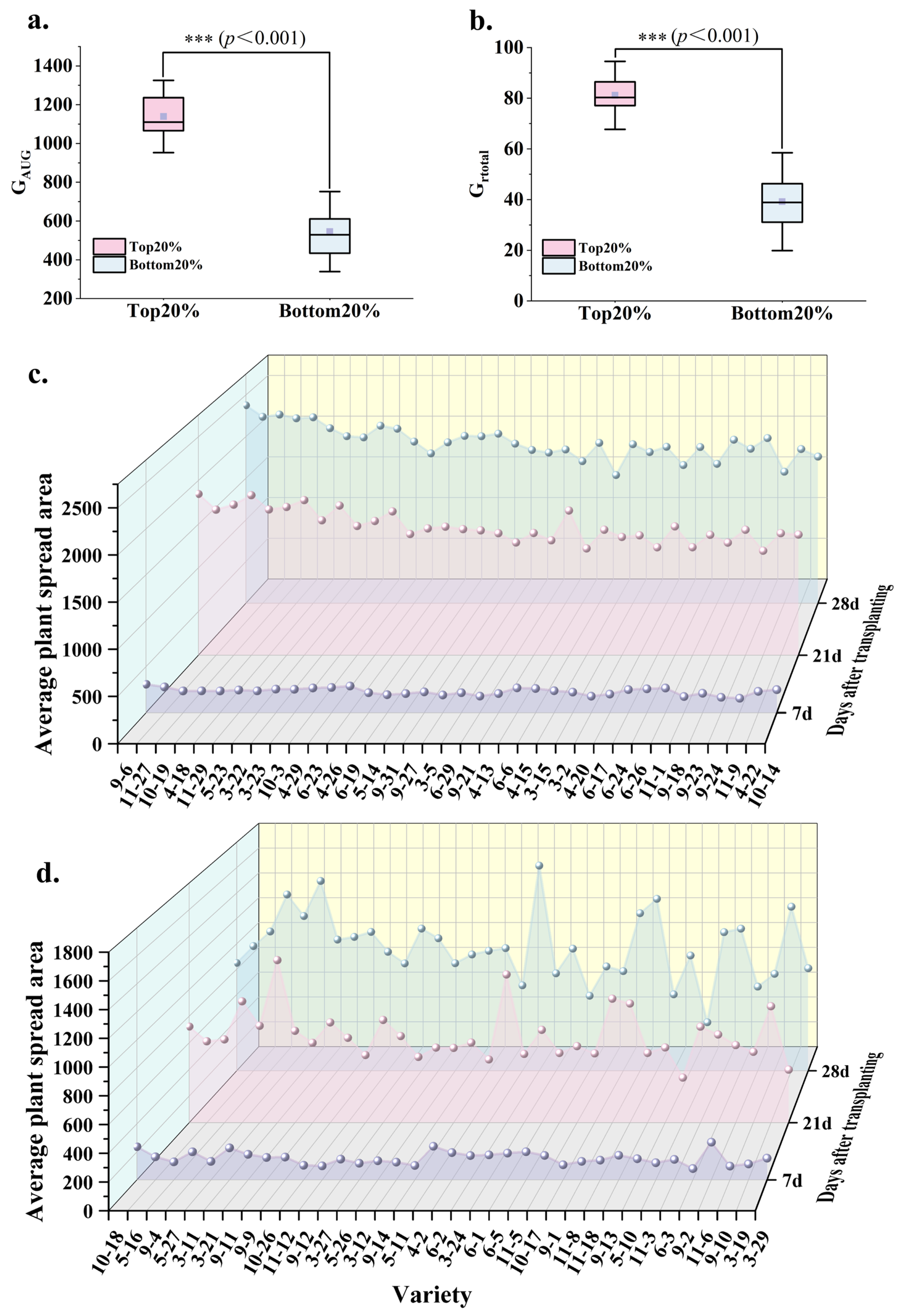
The top- and bottom-ranked 20% of varieties in the comprehensive evaluation ranking were compared and analyzed. As shown in Figure 9a,b, both growth indicators showed highly significant differences. The G_AUC values of the top 20% of the varieties were mainly concentrated around 1200, whereas those of the bottom 20% were mostly distributed between 400 and 700. This indicates that the top-ranked varieties in the comprehensive evaluation had greater cumulative growth and overall growth advantages during the 7–28 d observation period. The G_rtotal values of the top 20% of the varieties were mainly between 70 and 90, whereas those of the bottom 20% were between 30 and 50. This indicates that the top 20% of varieties had a faster overall growth rate during the 7–28 d period and showed greater early-seedling-growth potential.

Combined with the dynamic growth curves at the three time points (Figure 9c,d), the growth levels of the top 20% of the varieties were higher than those of the bottom 20% at 7, 21, and 28 d. At 28 d, the average plant canopy area of the top 20% of varieties was approximately 2500, indicating better growth performance at this time point. In contrast, the bottom 20% of varieties showed a relatively lower overall level at 28 d, with most varieties distributed between 1500 and 2000 and considerable differences among varieties. The top 20% of the varieties identified through the comprehensive evaluation showed clear advantages in G_AUC, G_rtotal, and dynamic growth patterns across the three time points, demonstrating that these varieties had high cumulative growth levels, fast overall growth rates, and superior seedling growth performance. In contrast, the bottom 20% of the varieties showed weaker overall growth performance and poorer growth stability within the germplasm collection.

3.5.3. Consistency Analysis Between Emergence and Growth Performance

To further analyze the relationship between emergence ability and the comprehensive level of seedling growth performance, the top 20% and bottom 20% of varieties were identified based on emergence indicators and comprehensive growth evaluation scores, respectively.

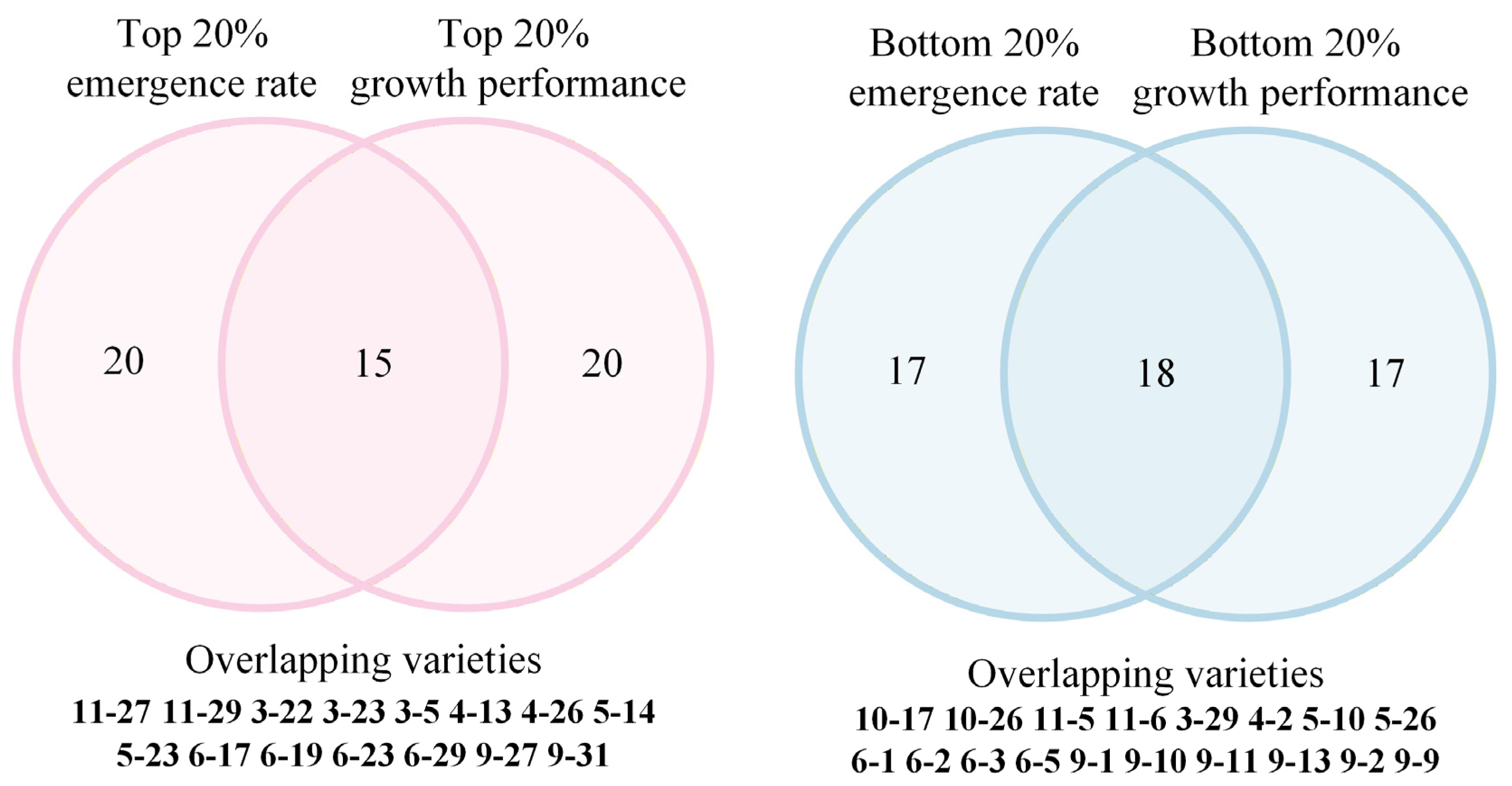
A Venn diagram was used to perform an overlap analysis of the two evaluation results, as shown in Figure 10. Among the top 20% of varieties, only 15 germplasm accessions overlapped in both emergence ability and growth performance, whereas many varieties showed outstanding performance in only one of the two dimensions. Among the bottom 20% of lower-performing varieties, 18 germplasm accessions overlapped in both poor emergence ability and weak growth performance, indicating that some varieties performed poorly in both emergence ability and early seedling growth.

4. Discussion

4.1. Model Optimization

UAV imaging technology and object detection models such as YOLO have been applied to crop object recognition. Studies on multi-domain agricultural imagery have shown that model selection should comprehensively consider different evaluation metrics. Among them, YOLOv11 exhibited relatively small performance variations under different spectral and image-quality conditions, demonstrating good stability [35]. This provided a reference for selecting YOLOv11 as the baseline model in this study. In addition, previous studies have shown that lightweight network optimization can reduce the number of model parameters and computational complexity. Meanwhile, it can maintain the detection performance of small-scale crop targets in complex field environments [36]. Based on this, YOLOv11 was lightweightly optimized in this study to improve model efficiency while maintaining high detection performance for small cauliflower seedling targets.

The C3k2 modules in stages P4 and P5 of the backbone were replaced with UIBBlock modules from MobileNetV4 to reduce the number of network parameters and computational complexity. Meanwhile, the P5 large-scale detection branch was removed, and only the P3 and P4 dual-scale detection heads were retained to enhance the detection capability of the model for small-scale targets. The P5 feature map had a relatively low resolution, which limited its ability to represent the spatial details of small seedling targets and increased computational redundancy. Therefore, removing the P5 detection head helped reduce unnecessary computations and lowered the risk of false detections. The introduction of the lightweight UIBBlock module further improved computational efficiency while maintaining the model’s feature representation capability, thereby enhancing its potential for real-time inference applications under field conditions.

The DualSlim-YOLO model maintained detection performance while increasing the inference speed from 56.18 FPS to 68.63 FPS, representing an improvement of approximately 22.16%. In addition, the model maintained good detection performance on external test images with no spatial overlap with the original dataset, indicating good generalization ability for the same crop. The mAP@0.5:0.95 at 7 days was lower than that at 21 and 28 days. This may be because the seedlings were smaller and had weaker boundary features at the early-growth stage, making localization errors more pronounced at higher IoU thresholds. Lightweight models have also been shown improve the applicability of edge-device deployment in field detection tasks for crops such as cabbage [37], potato seedlings [38], and maize tassels [39]. Therefore, in seedling-stage small-object detection tasks, reasonable adjustment of the detection-scale structure combined with lightweight feature extraction modules can achieve a good balance among detection performance, model complexity, and inference efficiency.

4.2. Emergence Rate Estimation and Dynamic Growth Monitoring

Automatic seedling recognition, estimation of emergence rates, and dynamic evaluation of early-growth performance are of great significance in crop breeding. In this study, the emergence rates and dynamic growth parameters of different cauliflower varieties were extracted using multitemporal UAV RGB imagery and an improved lightweight object detection model, enabling a comprehensive evaluation of seedling-stage growth performance. Existing studies have mostly focused on single-dimensional analyses, either estimating only seedling numbers [40,41] or evaluating seedling-stage growth based only on growth parameters [42,43]. This study found that integrating emergence rate and dynamic growth parameters enabled a more comprehensive analysis of seedling-stage growth differences (Figure 9). Among them, the top 20% of varieties in the comprehensive ranking showed significantly higher G_AUC, G_rtotal, and mean projected area at different time points than the bottom 20% of varieties, indicating that the comprehensive evaluation could effectively distinguish seedling-stage growth performance among different varieties. The emergence rate reflects the number of established seedlings of each variety, whereas the comprehensive growth evaluation reflects the early-growth status of the seedling population. A combination of these two methods can improve the accuracy and stability of variety screening.

As shown in Figure 10, the Venn overlap analysis between emergence rate and comprehensive growth evaluation showed that some varieties, such as 11-27, 11-29, and 3-22, were common to top 20% of the groups selected based on emergence rate and comprehensive growth evaluation. This indicates that some varieties have advantages in both emergence ability and seedling-stage growth performance. In contrast, varieties such as 10-17, 10-26, and 11-5 ranked in the bottom 20% for both emergence rate and growth performance, indicating that these varieties may have poor emergence and slow growth during the seedling stage. Some cultivars may exhibit a high emergence rate but weak overall growth, whereas others may exhibit good overall growth but a relatively low emergence rate. This indicates that a single indicator could not fully and objectively evaluate the comprehensive performance of cauliflower seedlings. Therefore, in the identification and evaluation of multiple cauliflower cultivars at the seedling stage, combining emergence rate estimation with the dynamic analysis of early growth can effectively identify superior cauliflower cultivars with stable emergence and outstanding early-growth potential, thereby demonstrating the advantages of the multi-feature fusion quantitative evaluation model.

In addition, the results of stepwise variable selection showed that E_decline and G_cv were not retained in the final regression model. This may be related to the correlations and information overlap among different emergence-rate and dynamic growth indicators. When the other variables were included in the model, Edecline and Gcv provided only limited additional contributions to the model. Variable selection can reduce redundant variables while retaining the key phenotypic information, thereby improving the simplicity and interpretability of the comprehensive evaluation model.

4.3. Limitations and Future Research Directions

This study used multi-temporal UAV imagery to monitor the emergence rate and seedling growth of different cauliflower varieties, effectively distinguishing varietal differences in emergence rate and early-growth traits. This provides reliable technical support for cauliflower germplasm identification and resource screening at the seedling stage.

However, this method still has certain limitations. DualSlim-YOLO has not yet been deployed on actual edge-computing platforms, and its inference efficiency and practical performance on resource-constrained devices require further evaluation. In addition, the plant spread area derived from rectangular bounding boxes of cauliflower seedlings in this study was used only as an approximate representation of canopy size. Future studies could extend the monitoring period to the entire growth cycle of cauliflower and incorporate field measurements to validate the accuracy and applicability of the estimated plant spread area.

5. Conclusions

This paper proposes a cauliflower seedling growth evaluation method based on UAV imagery and object detection. UAV images acquired at 7, 21, and 28 d were integrated with the DualSlim-YOLO model to achieve automatic cauliflower seedling identification, seedling counting, and batch extraction of seedling-stage phenotypic parameters. The DualSlim-YOLO model effectively reduced model complexity and improved inference efficiency while maintaining high detection accuracy, making it suitable for batch processing of UAV images and rapid seedling identification at the cauliflower seedling stage.

For emergence rate estimation, this study obtained the number of seedlings for different cultivars at three time points based on the seedling detection results and then calculated their emergence rates and dynamic variation characteristics. These results enabled rapid, nondestructive, and quantitative monitoring of the cauliflower emergence process. For growth analysis, this study combined UAV image ground resolution parameters to extract and comprehensively evaluate seedling-stage growth parameters of different cultivars, thereby achieving dynamic monitoring of the early-growth status of different cauliflower cultivars. The cross-validation results between emergence and growth indicated that a single emergence indicator could not fully reflect the comprehensive seedling-stage performance of cultivars, whereas integrating multidimensional phenotypic features enabled a more accurate evaluation of early-growth potential. This study provides efficient and nondestructive technical support for the precise monitoring, high-throughput phenotyping, and early screening of superior germplasm resources at the cauliflower seedling stage. It also provides a reference for intelligent monitoring of Brassicaceae vegetables at the seedling stage.

References

1. Zhou, H.; Li, Q.; Qin, B.; Min, H.; Liang, S.; Wang, X.; Cai, J.; Zhou, Q.; Huang, M.; Jiang, D.; et al. High-Throughput Wheat Seedling Phenotyping via UAV-Based Semantic Segmentation and Ground Sample Distance-Driven Pixel-to-Area Mapping. Comput. Electron. Agric. 2025, 238, 110819. [Google Scholar] [CrossRef] [Scilit]
2. Yang, G.J.; Liu, J.G.; Zhao, C.J.; Li, Z.H.; Huang, Y.B.; Yu, H.Y.; Xu, B.; Yang, X.D.; Zhu, D.; Zhang, X.; et al. Unmanned Aerial Vehicle Remote Sensing for Field-Based Crop Phenotyping: Current Status and Perspectives. Front. Plant Sci. 2017, 8, 1111. [Google Scholar] [CrossRef] [Scilit]
3. Maimaitijiang, M.; Sagan, V.; Sidike, P.; Daloye, A.M.; Erkbol, H.; Fritschi, F.B. Crop Monitoring Using Satellite/UAV Data Fusion and Machine Learning. Remote Sens. 2020, 12, 1357. [Google Scholar] [CrossRef] [Scilit]
4. Yue, J.; Yang, G.; Tian, Q.; Feng, H.; Xu, K.; Zhou, C. Estimate of Winter-Wheat Above-Ground Biomass Based on UAV Ultrahigh-Ground-Resolution Image Textures and Vegetation Indices. ISPRS J. Photogramm. Remote Sens. 2019, 150, 226–244. [Google Scholar] [CrossRef] [Scilit]
5. Johansen, K.; Morton, M.J.L.; Malbeteau, Y.; Aragon, B.; Al-Mashharawi, S.; Ziliani, M.G.; Angel, Y.; Fiene, G.; Negrão, S.; Mousa, M.A.A.; et al. Predicting Biomass and Yield in a Tomato Phenotyping Experiment Using UAV Imagery and Random Forest. Front. Artif. Intell. 2020, 3, 28. [Google Scholar] [CrossRef] [Scilit]
6. Barzin, R.; Kamangir, H.; Bora, G.C. Comparison of Machine Learning Methods for Leaf Nitrogen Estimation in Corn Using Multispectral UAV Images. Trans. ASABE 2021, 64, 2089–2101. [Google Scholar] [CrossRef] [Scilit]
7. Osco, L.P.; Junior, J.M.; Ramos, A.P.M.; Furuya, D.E.G.; Santana, D.C.; Teodoro, L.P.R.; Gonçalves, W.N.; Baio, F.H.R.; Pistori, H.; Junior, C.A.d.S.; et al. Leaf Nitrogen Concentration and Plant Height Prediction for Maize Using UAV-Based Multispectral Imagery and Machine Learning Techniques. Remote Sens. 2020, 12, 3237. [Google Scholar] [CrossRef] [Scilit]
8. Wilke, N.; Siegmann, B.; Postma, J.A.; Muller, O.; Krieger, V.; Pude, R.; Rascher, U. Assessment of Plant Density for Barley and Wheat Using UAV Multispectral Imagery for High-Throughput Field Phenotyping. Comput. Electron. Agric. 2021, 189, 106380. [Google Scholar] [CrossRef] [Scilit]
9. Li, B.; Xu, X.M.; Han, J.W.; Zhang, L.; Bian, C.S.; Jin, L.P.; Liu, J.G. The Estimation of Crop Emergence in Potatoes by UAV RGB Imagery. Plant Methods 2019, 15, 15. [Google Scholar] [CrossRef] [Scilit]
10. Xie, J.; Zhou, Z.; Zhang, H.; Zhang, L.; Li, M. Combining Canopy Coverage and Plant Height from UAV-Based RGB Images to Estimate Spraying Volume on Potato. Sustainability 2022, 14, 6473. [Google Scholar] [CrossRef] [Scilit]
11. Gao, M.; Yang, F.; Wei, H.; Liu, X. Automatic Monitoring of Maize Seedling Growth Using Unmanned Aerial Vehicle-Based RGB Imagery. Remote Sens. 2023, 15, 3671. [Google Scholar] [CrossRef] [Scilit]
12. Yang, T.; Zhu, S.; Zhang, W.; Zhao, Y.; Song, X.; Yang, G.; Yao, Z.; Wu, W.; Liu, T.; Sun, C.; et al. Unmanned Aerial Vehicle-Scale Weed Segmentation Method Based on Image Analysis Technology for Enhanced Accuracy of Maize Seedling Counting. Agriculture 2024, 14, 175. [Google Scholar] [CrossRef] [Scilit]
13. Sun, B.; Li, Y.; Huang, J.; Cao, Z.; Peng, X. Impacts of Variable Illumination and Image Background on Rice LAI Estimation Based on UAV RGB-Derived Color Indices. Appl. Sci. 2024, 14, 3214. [Google Scholar] [CrossRef] [Scilit]
14. Feng, Y.; Chen, W.; Ma, Y.; Zhang, Z.; Gao, P.; Lv, X. Cotton Seedling Detection and Counting Based on UAV Multispectral Images and Deep Learning Methods. Remote Sens. 2023, 15, 2680. [Google Scholar] [CrossRef] [Scilit]
15. Zang, H.; Wang, Y.; Peng, Y.; Han, S.; Zhao, Q.; Zhang, J.; Li, G. Automatic Detection and Counting of Wheat Seedling Based on Unmanned Aerial Vehicle Images. Front. Plant Sci. 2025, 16, 1665672. [Google Scholar] [CrossRef] [Scilit]
16. Ren, L.; Li, C.; Yang, G.; Zhao, D.; Zhang, C.; Xu, B.; Feng, H.; Chen, Z.; Lin, Z.; Yang, H. The Detection of Maize Seedling Quality from UAV Images Based on Deep Learning and Voronoi Diagram Algorithms. Remote Sens. 2024, 16, 3548. [Google Scholar] [CrossRef] [Scilit]
17. Tang, B.; Zhou, J.; Pan, Y.; Qu, X.; Cui, Y.; Liu, C.; Li, X.; Zhao, C.; Gu, X. Recognition of Maize Seedling under Weed Disturbance Using Improved YOLOv5 Algorithm. Measurement 2025, 242, 115938. [Google Scholar] [CrossRef] [Scilit]
18. Zhao, M.; Wang, D.; Zhang, G.; Cao, W.; Xu, S.; Li, Z.; Liu, X. Evaluating Maize Emergence Quality with Multi-Task YOLO11-Mamba and UAV-RGB Remote Sensing. Smart Agric. Technol. 2025, 12, 101351. [Google Scholar] [CrossRef] [Scilit]
19. Yu, G.; Wang, X.; Wang, L.; Dong, H.; Tang, T.; Ma, Y.; Qi, P. SD-MSL-YOLO: A Lightweight Model for Vegetable Pot Seedling Detection and Missing Seedling Localization. Comput. Electron. Agric. 2026, 246, 111597. [Google Scholar] [CrossRef] [Scilit]
20. Zheng, J.; Chen, Y.; Jin, J.; Huang, S.; Zhou, X.; Huang, W. An End-to-End Precision Phenotyping Framework: Rice Panicle Detection and Counting in Complex Fields via Lightweight DETR. AgriEngineering 2026, 8, 294. [Google Scholar] [CrossRef] [Scilit]
21. Feng, P.; Nie, Z.; Li, G. Field-Deployable Lightweight YOLOv8n for Real-Time Detection and Counting of Maize Seedlings Using UAV RGB Imagery. Front. Plant Sci. 2025, 16, 1639533. [Google Scholar] [CrossRef] [Scilit]
22. Anandakrishnan, J.; Sangaiah, A.K.; Darmawan, H.; Son, N.K.; Lin, Y.-B.; Alenazi, M.J.F. Precise Spatial Prediction of Rice Seedlings from Large-Scale Airborne Remote Sensing Data Using Optimized Li-YOLOv9. IEEE J. Sel. Top. Appl. Earth Obs. Remote Sens. 2025, 18, 2226–2238. [Google Scholar] [CrossRef] [Scilit]
23. Zeng, F.; Wang, R.; Jiang, Y.; Liu, Z.; Ding, Y.; Dong, W.; Xu, C.; Zhang, D.; Wang, J. Growth Monitoring of Rapeseed Seedlings in Multiple Growth Stages Based on Low-Altitude Remote Sensing and Semantic Segmentation. Comput. Electron. Agric. 2025, 232, 110135. [Google Scholar] [CrossRef] [Scilit]
24. Li, J.; Li, Y.; Qiao, J.; Li, L.; Wang, X.; Yao, J.; Liao, G. Automatic Counting of Rapeseed Inflorescences Using Deep Learning Method and UAV RGB Imagery. Front. Plant Sci. 2023, 14, 1101143. [Google Scholar] [CrossRef] [Scilit]
25. Li, J.; Zhu, C.; Yang, C.; Zheng, Q.; Wang, B.; Tu, J.; Zhang, Q.; Liu, S.; Wang, X.; Qiao, J. DM_CorrMatch: A Semi-Supervised Semantic Segmentation Framework for Rapeseed Flower Coverage Estimation Using UAV Imagery. Plant Methods 2025, 21, 54. [Google Scholar] [CrossRef] [Scilit]
26. Zhang, J.; Liu, J.; Zhang, D.; Yang, T.; Zhang, C.; Yu, Q.; Cui, X.; Fan, X.; Wang, X.-X. High-Throughput Phenotyping of Chinese Cabbage Using Multispectral Drone Imagery and Deep Learning for Morphological, Color, and Nutritional Traits across Growth Stages. Sci. Hortic. 2025, 346, 114172. [Google Scholar] [CrossRef] [Scilit]
27. Shi, H.; Liu, C.; Wu, M.; Zhang, H.; Song, H.; Sun, H.; Li, Y.; Hu, J. Real-Time Detection of Chinese Cabbage Seedlings in the Field Based on YOLO11-CGB. Front. Plant Sci. 2025, 16, 1558378. [Google Scholar] [CrossRef] [Scilit]
28. Lee, C.-J.; Yang, M.-D.; Tseng, H.-H.; Hsu, Y.-C.; Sung, Y.; Chen, W.-L. Single-Plant Broccoli Growth Monitoring Using Deep Learning with UAV Imagery. Comput. Electron. Agric. 2023, 207, 107739. [Google Scholar] [CrossRef] [Scilit]
29. Hayashi, H.; Shimazaki, H.; Korei, R.; Oki, K. Locating Open-Field Broccoli Plants with Unmanned Aerial Vehicle Photogrammetry and Object Detection Algorithm: A Practical Prediction Approach. Sens. Mater. 2023, 35, 3777–3790. [Google Scholar] [CrossRef] [Scilit]
30. Kierdorf, J.; Junker-Frohn, L.V.; Delaney, M.; Donoso Olave, M.; Burkart, A.; Jaenicke, H.; Muller, O.; Rascher, U.; Roscher, R. GrowliFlower: An Image Time-Series Dataset for Growth Analysis of Cauliflower. J. Field Robot. 2023, 40, 173–192. [Google Scholar] [CrossRef] [Scilit]
31. Kierdorf, J.; Stomberg, T.T.; Drees, L.; Rascher, U.; Roscher, R. Investigating the Contribution of Image Time Series Observations to Cauliflower Harvest-Readiness Prediction. Front. Artif. Intell. 2024, 7, 1416323. [Google Scholar] [CrossRef] [Scilit]
32. Cheng, S.; Wu, S.; Shao, Q.; Chen, M.; Liu, J.; Qiu, B.; Zhu, H. High-Throughput Phenotypic Analysis of Plant and Curd Growth Dynamics during the Whole Growth Period of Cauliflower Based on Instance Segmentation. Front. Plant Sci. 2026, 17, 1836813. [Google Scholar] [CrossRef] [Scilit]
33. Yue, Y.; Zhao, A. YOLOv11-Seg-SSC: Soybean Seedling Segmentation and Spatial Localization from Low-Altitude UAV Imagery. Agronomy 2026, 16, 536. [Google Scholar] [CrossRef] [Scilit]
34. Qin, D.; Leichner, C.; Delakis, M.; Fornoni, M.; Luo, S.; Yang, F.; Wang, W.; Banbury, C.; Ye, C.; Akin, B.; et al. MobileNetV4: Universal Models for the Mobile Ecosystem. In Computer Vision—ECCV 2024; Leonardis, A., Ricci, E., Roth, S., Russakovsky, O., Sattler, T., Varol, G., Eds.; Springer: Cham, Switzerland, 2024; Volume 15098, pp. 78–96. [Google Scholar] [CrossRef] [Scilit]
35. Rana, S.; Hensel, O.; Nasirahmadi, A. From Vineyard to Vision: Multi-Domain Analysis and Mitigation of Grape Cluster Detection Failures in Complex Viticultural Environments. Results Eng. 2026, 29, 108833. [Google Scholar] [CrossRef] [Scilit]
36. Wu, H.Q.; Guan, M.X.; Chen, J.N.; Pan, Y.; Zheng, J.Y.; Jin, Z.C.; Li, H.; Tan, S.Y. OE-YOLO: An EfficientNet-Based YOLO Network for Rice Panicle Detection. Plants 2025, 14, 1370. [Google Scholar] [CrossRef] [Scilit]
37. Zhao, R.; Luo, R.; Ding, X.; Cui, J.; Yi, B. Lightweight YOLOv11n-Based Detection and Counting of Early-Stage Cabbage Seedlings from UAV RGB Imagery. Horticulturae 2025, 11, 993. [Google Scholar] [CrossRef] [Scilit]
38. Wang, L.; Wang, G.; Yang, S.; Liu, Y.; Yang, X.; Feng, B.; Sun, W.; Li, H. Research on Improved YOLOv8n-Based Potato Seedling Detection in UAV Remote Sensing Images. Front. Plant Sci. 2024, 15, 1387350. [Google Scholar] [CrossRef] [Scilit]
39. Han, Y.; Wang, X.; Niu, L.; Shi, S.; Gao, Y.; Gong, K.; Zhang, X.; Zheng, J. OTB-YOLO: An Enhanced Lightweight YOLO Architecture for UAV-Based Maize Tassel Detection. Plants 2025, 14, 2701. [Google Scholar] [CrossRef] [Scilit]
40. Chen, H.; Chen, H.; Huang, X.; Zhang, S.; Chen, S.; Cen, F.; He, T.; Zhao, Q.; Gao, Z. Estimation of Sorghum Seedling Number from Drone Image Based on Support Vector Machine and YOLO Algorithms. Front. Plant Sci. 2024, 15, 1399872. [Google Scholar] [CrossRef] [Scilit]
41. Zhang, C.; Sun, X.; Xuan, S.; Zhang, J.; Zhang, D.; Yuan, X.; Fan, X.; Suo, X. Monitoring of Broccoli Flower Head Development in Fields Using Drone Imagery and Deep Learning Methods. Agronomy 2024, 14, 2496. [Google Scholar] [CrossRef] [Scilit]
42. Parker, T.A.; Palkovic, A.; Gepts, P. Determining the Genetic Control of Common Bean Early-Growth Rate Using Unmanned Aerial Vehicles. Remote Sens. 2020, 12, 1748. [Google Scholar] [CrossRef] [Scilit]
43. Borra-Serrano, I.; De Swaef, T.; Quataert, P.; Aper, J.; Saleem, A.; Saeys, W.; Somers, B.; Roldán-Ruiz, I.; Lootens, P. Closing the Phenotyping Gap: High-Resolution UAV Time Series for Soybean Growth Analysis Provides Objective Data from Field Trials. Remote Sens. 2020, 12, 1644. [Google Scholar] [CrossRef] [Scilit]
Figure 1. Overall workflow of this study.
Agriculture 16 01883 g001
Figure 2. Network architecture of the proposed model.
Agriculture 16 01883 g002
Figure 3. Extraction of emergence-rate and seedling-growth parameters from UAV RGB imagery.
Agriculture 16 01883 g003
Figure 4. Time-point-specific AP on the independent test set. (a) mAP@0.5. (b) mAP@0.5:0.95.
Agriculture 16 01883 g004
Figure 5. Comparison of detection results before and after model improvement.
Agriculture 16 01883 g005
Figure 6. Cauliflower seedling detection process and dynamic emergence-rate monitoring results based on DualSlim-YOLO. (a) Visualization of the cauliflower seedling detection process. (b) Dynamic changes in emergence rates among different varieties.
Agriculture 16 01883 g006
Figure 7. Heatmaps of dynamic changes in emergence rates of different varieties at three time points. (a) Heatmap of emergence rates for the top 20% of varieties. (b) Heatmap of emergence rates for the bottom 20% of varieties.
Agriculture 16 01883 g007
Figure 8. PCA results of the comprehensive evaluation indicators for cauliflower seedling emergence rate and growth performance. (a) Pearson correlation heatmap of the evaluation indicators. (b) Contribution rate and cumulative contribution rate of the PCs. (c) Bubble plot of PC loadings.
Agriculture 16 01883 g008
Figure 9. Analysis of seedling growth differences among varieties based on the comprehensive evaluation. (a) Comparison of GAUC between the top 20% and bottom 20% of varieties in the comprehensive evaluation. (b) Comparison of Grtotal between the top 20% and bottom 20% of varieties in the comprehensive evaluation. (c) Dynamic changes in growth performance of the top 20% of varieties at the three time points. (d) Dynamic changes in growth performance of the bottom 20% of varieties at the three time points.
Agriculture 16 01883 g009
Figure 10. Overlap analysis of the top 20% and bottom 20% of varieties based on emergence rate and growth performance.
Agriculture 16 01883 g010