


Abstract
Against the backdrop of increasing global food security pressures and tightening resource–environment constraints, enhancing grain production efficiency has become a focal international concern. Based on panel data from 16 cities in Shandong Province, China, spanning 2013 to 2022, this study employs the DEA–Malmquist index, SBM model, and Spatial Durbin model to measure grain production efficiency and analyze its spatiotemporal evolution and influencing factors. The findings reveal that Shandong’s grain production efficiency has generally improved but exhibits a spatial differentiation pattern of “higher in Western Shandong, lower in Eastern Shandong,” with significant positive spatial correlation and agglomeration effects. Mechanization significantly boosts efficiency, while urbanization, excessive fertilizer and pesticide use, and labor surplus exert notable negative impacts. This research clarifies the spatial spillover mechanisms and key constraints of efficiency, providing scientific evidence and practical guidance for optimizing agricultural resource allocation, promoting regional collaborative innovation, and formulating differentiated food security policies in Shandong Province and other regions with similar natural–economic conditions.
1. Introduction
Against the backdrop of global climate change and increasing resource and environmental constraints, improving grain production efficiency has become an important way to ensure national food security [1]. Located in the eastern coastal area of China, Shandong Province has diverse terrain including mountains, hills, and plains, making it a major grain-producing region. In 2023, Shandong’s GDP exceeded 9 trillion CNY (12,535.69 billion USD) for the first time, with the gross output value of agriculture, forestry, animal husbandry, and fishery reaching 1253.19 billion CNY (174.55 billion USD), highlighting its pivotal role in national grain production [2]. However, the traditional extensive growth path has become unsustainable, and there is an urgent need to promote agricultural transformation through technological upgrading and model innovation.
Scholars have extensively researched grain production efficiency. In the field of technical efficiency, Farrell provided a foundational work, interpreting technical efficiency as the ratio of theoretical minimum cost to actual cost [3], while Leibenstein defined it from the output perspective as the ratio of actual output to maximum possible output [4]. Regarding measurement methods, the C-D production function proposed by Cobb and Douglas pioneered quantitative analysis [5], and Coelli constructed a time-varying stochastic frontier production function (SFPF) [6]. According to Liu and Mao, Chinese scholars have mainly relied on two methodological systems: Stochastic Frontier Analysis (SFA) and Data Envelopment Analysis (DEA) [7]. For instance, Wang et al. applied a stochastic frontier production function approach to reveal the spatial–temporal heterogeneity of urban construction land allocation efficiency in China’s urban agglomerations [8]. However, in this study, we majorly focus on DEA, which is a non-parametric approach to evaluate the relative efficiency of a group of decision-making units (DMUs). DEA models have been widely adopted in existing research, and their frameworks and extended forms keep evolving continuously. For example, Liu et al. evaluated China’s grain production efficiency based on the super-efficiency DEA method [9]; Yin et al. used the Slacks-Based Measure (SBM) model to measure Chinese total grain production efficiency under climate change [10]; and Zhang and Jia analyzed the grain production efficiency of five major grain-producing provinces using the DEA–Malmquist index model [11]. In recent years, DEA has achieved prominent applications in research on spatial–temporal differentiation. Li et al. studied spatial variations in agricultural efficiency in Iran [12]; Frei et al. revealed the impact of climate and potassium nutrition on crop yields based on a 30-year Swiss long-term fertilization experiment [13]; scholars Jin and Han analyzed the regional pattern changes and driving factors of China’s grain production [14]; Shao et al. revealed a distinct trend of “northward and westward” spatial restructuring in grain production [15]. A wide range of spatial analytical approaches have been extensively adopted in agricultural production system research. In early studies, scholars such as Liu et al. mainly relied on global and local Moran’s indices, Getis–Ord hot spot analysis and standard deviational ellipses to identify the agglomeration and differentiation patterns of grain efficiency across regions [16]. To further quantify cross-regional interactive relationships, spatial econometric panel models were used by scholars, such as Jing et al., to decompose local direct effects and interregional spatial spillover effects based on multi-year panel datasets [17]. Regarding influencing factors, Ordóñez et al. systematically analyzed the interactive driving effects of weather and technology on soybean production in the United States [18]; Dong et al. studied the contributions of planting density, nitrogen application, and other factors to rice yield changes [19]; according to Zhang, land is the core determinant shaping grain output performance across regions [20]; Luo et al. found that the amount of agricultural and the level of agricultural technology present a “U-shaped” trend for production agglomeration [21]; Wei and Lu revealed a positive correlation between farmers’ machinery ownership and grain production efficiency [22]; Deng and Zhu found that conservation tillage combinations significantly improved grain production efficiency [23]; and Zhang et al. found that agricultural subsidy reform policies significantly promoted the improvement of grain production efficiency [24].
Although existing research has laid a solid theoretical foundation and provided abundant empirical evidence, some questions remain. First, most existing studies are carried out at the national macro scale (e.g., Ding et al.) or concentrate on a single grain crop (e.g., Li and Cui) [25,26], and there is a lack of systematic efficiency measurement and spatial–temporal evolution analysis specifically for Shandong Province, an important grain-producing region. Second, as Liu et al. argued, most existing evaluations of grain production efficiency merely depict rudimentary spatial clustering patterns, while failing to employ spatial econometric frameworks [27]. Third, Wang Helong’s research findings indicate that advances in green technology are one of the primary drivers of growth [28]. Traditional efficiency evaluations often focus only on desirable outputs such as grain yield, while ignoring undesirable outputs such as agricultural carbon emissions, making it difficult to fully reflect the true level of efficiency under the background of green and sustainable development. Furthermore, there are disagreements in existing conclusions regarding the direction and magnitude of the effects of modern factors such as mechanization, digitalization, and urbanization.
To further investigate these issues, this paper uses panel data from 16 prefecture-level cities in Shandong Province from 2013 to 2022, constructs an evaluation system that includes input indicators and output indicators, and comprehensively applies the SBM model, DEA–Malmquist index, spatial autocorrelation analysis, and the spatial Durbin model (SDM) to systematically reveal the static level, dynamic evolution trend, spatial correlation pattern, and spatial spillover effects of influencing factors of grain production efficiency in Shandong Province. The study aims to answer three core questions: What spatial–temporal evolution characteristics does grain production efficiency in Shandong Province present? Does significant spatial agglomeration and spillover effects exist? What are the direct and indirect effects of different factors on efficiency?
The contributions of this paper are threefold. First, it incorporates agricultural carbon emissions into the grain production efficiency evaluation system, addressing the shortcoming of traditional efficiency measurements that ignore undesirable outputs, and making the evaluation more consistent with the concepts of green agriculture and sustainable development. Second, it constructs a comprehensive analytical framework by combining the DEA–Malmquist index model with spatial autocorrelation and cold–hot spot analysis, revealing the temporal dynamics and spatial evolution characteristics of efficiency from both static and dynamic perspectives. Third, it uses the spatial Durbin model to quantify the direct, indirect, and total effects of different factors on grain production efficiency, deeply revealing the influence mechanisms of various factors at different spatial scales, and providing a refined scientific basis for formulating differentiated regional agricultural policies.
2. Materials and Methods
2.1. Study Area, Model Construction, and Data
2.1.1. Overview of the Study Area
Shandong Province is located in the coastal area of Eastern China, bordering the Yellow Sea to the east. Its terrain is diverse: the central and eastern parts are dominated by plains, with the Yellow River Delta possessing fertile soil and serving as a major grain-producing area, while the western and southern regions are mostly mountainous and hilly, which benefits ecological conservation. Land resources are characterized by high-intensity cultivation and limited reserve space. The main soil types are fluvo-aquic soil (Fluvisols, WRB), brown soil (Cambisols, WRB), and cinnamon soil (Calcic Cambisols, WRB), accounting for 48%, 24%, and 19% of the cultivated area, respectively. Hydrologically, Shandong sits at the junction of the Yellow River, Huai River, and Hai River basins, with a dense water network and important lakes, such as Nansi Lake and Dongping Lake. The average annual precipitation is approximately 676.5 mm, and total water resources amount to 30.58 billion m3. The annual inflow of the Yellow River fluctuates significantly, highlighting the need for inter-basin water transfer. The climate is warm-temperate monsoon, with an average annual temperature of 11–14 °C, a frost-free period of 180–220 days, annual sunshine of 2290–2890 h, and precipitation of 550–950 mm, which is concentrated in summer (posing flood risks) while droughts often occur in winter, spring, and late autumn. Socioeconomically, at the end of 2022, Shandong had a permanent resident population of 101.6279 million, administering 16 prefecture-level cities. In 2023, its GDP exceeded 9 trillion yuan for the first time, reaching 9.2069 trillion yuan with a growth rate of 6.0%. The value added of the primary, secondary, and tertiary industries was 650.6 billion, 3.5988 trillion, and 4.9575 trillion yuan, respectively. The per capita disposable income of residents was 39,890 yuan (51,571 yuan for urban residents and 23,776 yuan for rural residents). Among its cities, Qingdao, Jinan, and Yantai ranked as the top three in GDP, reaching 1.576 trillion yuan, 1.276 trillion yuan, and 1.016 trillion yuan, respectively, with growth rates mostly between 5% and 7%. Regional development shows a pattern of leading cities driving growth, accelerated transformation in traditional industrial cities, and gradually narrowing disparities.
In summary, although Shandong Province possesses favorable agricultural natural conditions and holds an important position in grain production, it also faces practical challenges such as uneven spatiotemporal distribution of water resources, frequent droughts and floods, a notable urban–rural income gap, and high-intensity cultivated land use. Therefore, systematically evaluating the spatiotemporal patterns of grain production efficiency in this province and its influencing factors is of great practical significance for optimizing resource allocation and ensuring regional food security.
2.1.2. Evaluation Index System Construction
Following the principles of comprehensiveness, representativeness, comparability, availability, scientificity, and goal orientation, and drawing on the studies of Qin et al. [29], Zhang et al., Huang et al. [30], and Liu et al. [31], an indicator system was constructed with six input indicators and two output indicators. Table 1 presents descriptive statistics of the input–output data for grain production in Shandong Province from 2013 to 2022.
Table 1.
Evaluation index system of grain production efficiency in Shandong Province.
2.1.3. Data Sources and Processing
This study focuses on 16 prefecture-level cities in Shandong Province, covering the period from 2013 to 2022. The data were obtained from the Shandong Statistical Yearbook (various editions, 2014–2023) and the National Economic and Social Development Statistical Bulletins of each city. One data limitation is missing data for agricultural employment and effective irrigated area in 2022. However, existing evidence indicates that these two indicators only experience slight annual variations, rendering linear interpolation a feasible imputation technique. Therefore, we filled the data gaps using the approach proposed by Emmendorfer. Second, as the prefecture-level city of Laiwu was abolished and merged into Jinan in December 2018, data for Laiwu from 2013 to 2018 were merged into Jinan following Zhou [32]. Collectively, these two categories of missing observations account for 3.75% of the total sample.
We attempted to extend the research period to 2023 and 2024 by collecting the latest municipal statistical bulletins. However, in 2023–2024, efficiency levels fluctuated a lot and showed extreme outliers, with many places’ efficiency numbers going beyond historically reasonable ranges. Within the baseline sample of 2013–2022, city-level grain production efficiency generally fluctuated steadily between 0.62 and 1.53, and most observations were concentrated in the range of 0.75–0.98. After extending the research period to 2024, however, drastic jumps emerged. For instance, Rizhao’s TE sharply surged to 1.6351 in 2024, far exceeding its maximum historical level during 2013–2022; meanwhile, Zibo, Dezhou, and Linyi maintained persistently low efficiency and experienced further declines in 2023, breaking their long-term stable intervals. In addition, the provincial average TE showed erratic volatility, dropping from 0.5912 in 2022 to 0.5800 in 2023 before rebounding sharply to 0.7196 in 2024. Such unreasonable drastic swings and outlier values originate from structural data defects: the suspension of city-level separate statistics for agriculture, forestry, animal husbandry, and fishery employment after 2022 and incomplete pesticide input data for 2024, together with the lagged shocks of public health emergencies. These issues distort the construction of the production frontier in the SBM model, leading to unreliable efficiency estimations.
Sharp efficiency surges and extreme outliers in 2023–2024 arise from two unavoidable data limitations. First, following the adjustment of national statistical accounting standards after 2022, official yearbooks no longer publish independent statistical data on employment in agriculture at the city level, while pesticide input data are unavailable for 2024. Second, research by Zhang and Liu De shows that the lagged effects of the pandemic, frequent extreme weather events, and adjustments to agricultural policies after 2022 have led to a large number of extreme observed values in grain production and input indicators [33]. Due to irreconcilable inconsistencies in statistical standards and systemic data gaps, this study restricts its research window to 2013–2022 for unified indicators and trustworthy estimation outcomes.
Agricultural carbon emissions (the undesirable output) were calculated using the emission coefficient method. The emission factors were adopted from the Intergovernmental Panel on Climate Change (IPCC), the Institute of Agricultural Resources and Regional Planning of Nanjing Agricultural University, Oak Ridge National Laboratory (USA), and the College of Biology and Technology of China Agricultural University. The total agricultural carbon emission E was calculated as:
where ei is the carbon emission from each carbon source, Ti is the amount of each carbon source, and δi is the corresponding emission coefficient (see Table 2). Conversion factors included: grain sown area (3.126 kg/hm2 = 0.003126 t/hm2), effective irrigated area (25 kg/hm2 = 25 t/1000 hm2), pesticide application (4.9341 kg/kg = 4.9341 t/t), and fertilizer application (0.8956 kg/kg = 0.8956 t/t).
Table 2.
Emission coefficients of various carbon emission sources.
2.2. Research Methodology
2.2.1. Nomenclature
All mathematical notations used in the Super-SBM model, Malmquist index, spatial autocorrelation test and spatial econometric models are systematically defined in the following Table 3 for reader convenience.
Table 3.
List of mathematical notations (Note: Full results for all years are available in Table A1 (Appendix A.1)).
2.2.2. SBM Model (Static Efficiency Analysis)
Data Envelopment Analysis (DEA), initially introduced by Charnes [34], is a non-parametric approach employing linear programming to assess the efficiency of homogeneous DMUs without the need for predetermined weights, thereby ensuring high objectivity and scientific validity. The SBM model, proposed by Tone [35], is a non-radial efficiency evaluation model within the DEA framework. It overcomes the overestimation problem of traditional radial models (e.g., CCR/BCC) by directly considering the slack variables of inputs and outputs. Assuming variable returns to scale, the SBM model is specified as follows:
where is the efficiency value of the DMU; m is the number of inputs; s1 and s2 are the numbers of desirable and undesirable outputs; is the input slack; and are the slacks for desirable and undesirable outputs; Xi0, , and are the observed input, desirable output, and undesirable output of DMU0; and λ is the intensity vector. When = 1 and all slacks are zero, the DMU is DEA-efficient; when < 1, the DMU is inefficient and improvements are possible. The model yields technical efficiency (TE), pure technical efficiency (PTE), and scale efficiency (SE). Calculations were performed using MaxDEA Ultra 8 software.
2.2.3. DEA–Malmquist Index Model (Dynamic Analysis)
In order to analyze the change in productivity across time, Malmquist [36] constructed the distance function in 1953 and proposed the concept of Malmquist index for the first time. Fare et al. [37] further developed and transformed the Malmquist index in 1994 and combined it with DEA theory effectively. The DEA–Malmquist index is a non-parametric tool for measuring dynamic changes in production efficiency. It decomposes total factor productivity change (TFPCH) into technical efficiency change (EFFCH) and technological change (TECHCH). Under variable returns to scale, EFFCH can be further decomposed into pure technical efficiency change (PECH) and scale efficiency change (SECH).
The Malmquist productivity index from period t to t + 1 is defined as:
where Dt(xt, yt) and Dt + 1(xt + 1, yt + 1) are the distance functions. An index greater than 1 indicates productivity growth. The decomposition is:
TFPCH = EFFCH × TECHCH = (PECH × SECH) × TECHCH
When TFPCH > 1, total factor productivity increases; when TFPCH < 1, it decreases. If EFFCH > 1, technical efficiency improves; and if TECHCH > 1, technological progress contributes to productivity growth. The DEA–Malmquist index was computed using DEAP 2.1 software.
2.2.4. Spatial Autocorrelation Analysis
Global Moran’s I was used to measure the overall spatial clustering of grain production efficiency across the 16 cities. The formula is:
where n is the number of spatial units (16 cities), yi and yj are the efficiency values of cities i and j, ȳ is the mean, wij is the spatial weight matrix (queen contiguity matrix), and S is the variance. Moran’s I ranges from −1 to 1; positive values indicate positive spatial autocorrelation.
Local Moran’s I was used to identify local spatial clusters and outliers. The results were visualized using Moran scatterplots, which classify cities into four quadrants: high–high (H-H), low–low (L-L), low–high (L-H), and high–low (H-L). Additionally, the Getis–Ord Gi* statistic implemented in ArcGIS 10.2 was used to identify statistically significant hot spots (high-value clusters) and cold spots (low-value clusters).
2.2.5. Spatial Econometric Models
Three spatial panel models were considered: the spatial Durbin model (SDM), Spatial Autoregressive Model (SAR), and Spatial Error Model (SEM). The spatial panel model serves as the core methodological tool in this study due to its technical advantages in capturing spatial dependencies, enhancing data analytical capabilities, and deepening the identification of spatial heterogeneity. The construction of its foundational model adheres to the following paradigm:
In the above formula, y is the dependent variable, X is the independent variable, W1y denotes the spatial lagged dependent variable, is the spatial autoregressive coefficient, β is the coefficient, and θ is the coefficient vector representing the spatial lagged effect of X on y. In the below formulae, W2Xθ denotes the influence of independent variables from neighboring regions on the local dependent variable; μ is the disturbance term; λ is the error coefficient for the spatial spillover effect of neighboring regions on local grain production efficiency; ε is the random error term; and W1, W2, and W3 are the spatial weight matrices. The spatial econometric models include the following types:
The spatial Durbin model (SDM), when λ = 0:
The Spatial Autoregressive Model (SAR), when λ = 0 and θ = 0:
The Spatial Error Model (SEM), when p = 0 and θ = 0:
where y is the dependent variable (TFPCH), X is the matrix of independent variables, W is the spatial weight matrix (queen contiguity), ρ and λ are spatial autocorrelation coefficients, β and θ are parameter vectors, and ϵ is the error term. When λ = 0, the model reduces to SDM; when λ = 0 and θ = 0, it reduces to SAR; when ρ = 0 and θ = 0, it reduces to SEM. Model selection was performed using LM tests, LR tests, Wald tests, and Hausman test. The Hausman test (p = 0.032) favored a fixed-effects model. LR and Wald tests both rejected the null that SDM simplifies to SAR or SEM (p < 0.001), thus the SDM with both individual and time fixed effects (double fixed) was chosen. To interpret the SDM results, the total effect was decomposed into direct effect (impact within the same city) and indirect effect (spatial spillover to neighboring cities). All spatial analyses were performed using Stata 17.0.
3. Results
3.1. Static and Dynamic Efficiency of Grain Production
3.1.1. Static Efficiency Based on the SBM Model
Using the SBM model described in Section 2.2.2, the grain production efficiency of 16 prefecture-level cities in Shandong Province from 2013 to 2022 was calculated. Table 4 presents the efficiency values for selected years. In 2022, four cities—Jinan, Dezhou, Binzhou, and Heze—achieved efficiency scores exceeding one, indicating DEA-efficient status. Among them, Heze recorded the highest value (1.5292). In contrast, Weihai and Dongying exhibited relatively low efficiency (0.7712 and 0.8243, respectively), suggesting substantial room for improvement.
Table 4.
Descriptive statistics of input–output variables for grain production in Shandong Province. (Note: Full results for all years are available in Table A2 (Appendix A.2)).
To better evaluate the overall trend, the average efficiency values for all cities across the study period are summarized in Table 5. The average technical efficiency (TE) increased from 0.8455 in 2013 to 0.9605 in 2022, representing a rise of approximately 13.6%. Pure technical efficiency (PTE) fluctuated considerably, reaching 1.1771 in 2018 and 1.3310 in 2022, while scale efficiency (SE) decreased from 0.9314 to 0.8502 over the same period. These results indicate that although overall grain production efficiency in Shandong Province has shown an upward trend, the decline in scale efficiency and the volatility in pure technical efficiency suggest that further optimization in technology application and resource allocation is needed.
Table 5.
Average value of grain production efficiency among the prefecture-level cities in Shandong Province from 2013 to 2022.
3.1.2. Dynamic Analysis Using the DEA–Malmquist Index
To reveal the trends and drivers of productivity change, the DEA–Malmquist index was applied. Figure 1 presents the annual TFPCH (total factor productivity change) and its decomposition for Shandong Province from 2013 to 2022. The average TFPCH over the entire period was 0.9962, slightly below one, indicating a marginal overall decline. However, positive growth was observed in three periods: 2015–2016 (1.0286), 2017–2018 (1.0486), and 2021–2022 (1.0206). The highest value occurred in 2017–2018, driven by both technical efficiency improvement (EFFCH = 1.0303) and technological progress (TECHCH = 1.0148).
Figure 1.
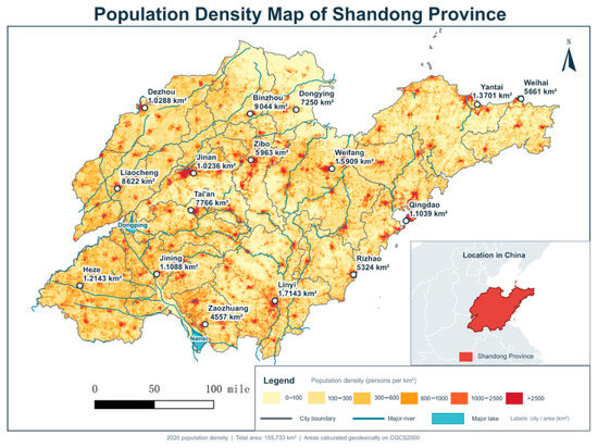
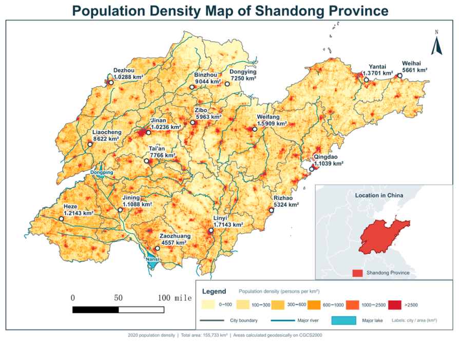
Population density map of Shandong Province.
Table 6 reports the decomposition of TFPCH for each period. The average values of pure technical efficiency change (PECH) and scale efficiency change (SECH) were close to one, suggesting relative stability. However, TECHCH fluctuated notably, reaching 1.1460 in 20182019, which offset declines in other components. These findings im ply that technological progress has been the primary driver of productivity growth, whereas efficiency changes have contributed less.
Table 6.
Dynamic calculation results of various cities in Shandong Province.
3.2. Spatial Evolution Characteristics of Grain Production Efficiency
3.2.1. Global and Local Spatial Autocorrelation
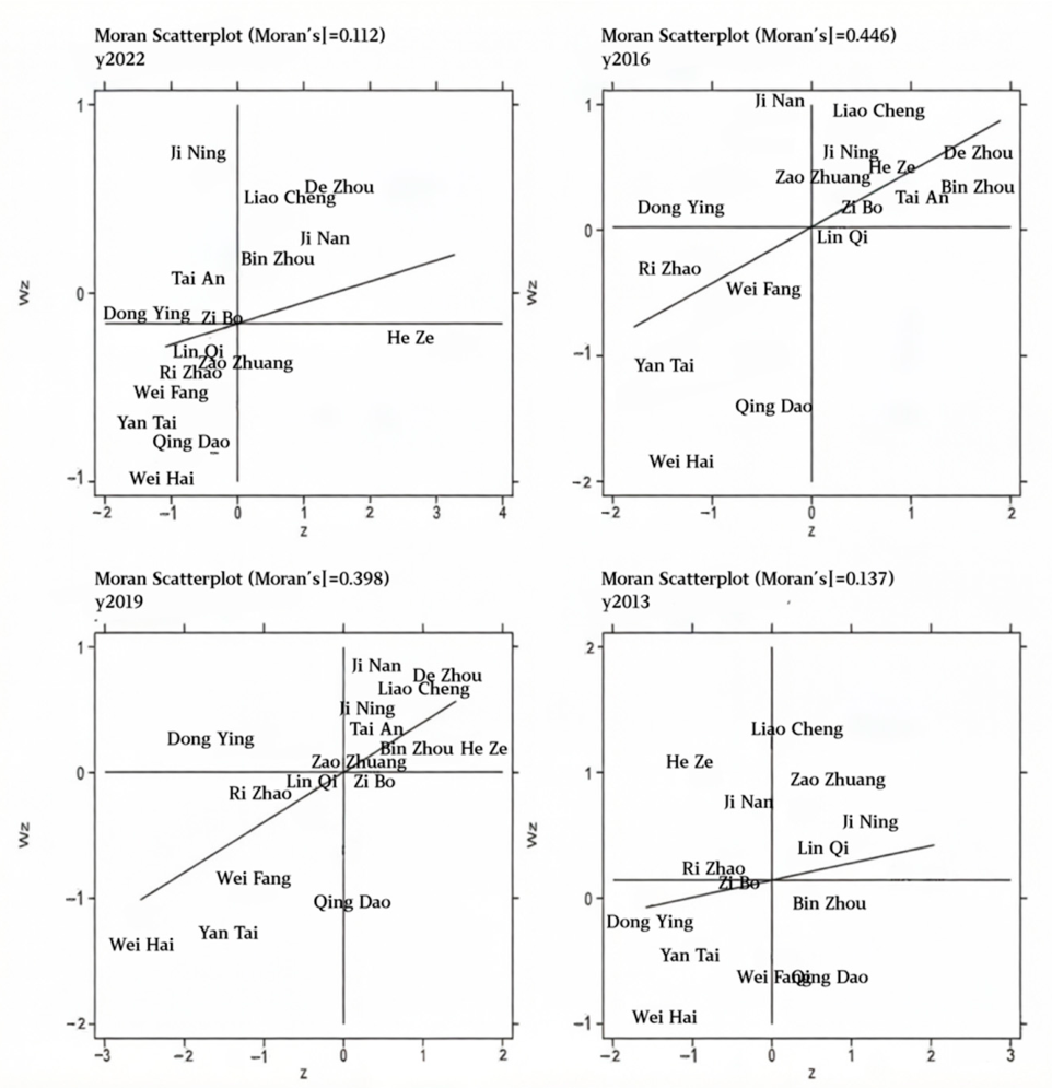
Global Moran’s I was calculated to test for spatial autocorrelation. As shown in Table 7, most years exhibited positive and statistically significant Moran’s I values. The index increased from 0.137 in 2013 (not significant) to 0.446 in 2016 (p < 0.01), indicating strengthening spatial clustering. Significant positive autocorrelation was also found in 2014, 2015, 2017, 2019, 2020, and 2021 (p < 0.05 or better). These results confirm that grain production efficiency in Shandong Province is not randomly distributed but exhibits spatial dependence.
Table 7.
Global autocorrelation inspection of grain production efficiency in all prefecture-level cities in Shandong Province from 2013 to 2022.
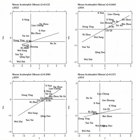
Local spatial autocorrelation was further examined using Moran scatterplots (Figure 2). Cities were classified into four quadrants: high–high (H-H), Low–Low (L-L), low–high (L-H), and High–Low (H-L). In 2013, H-H clusters included Liaocheng, Zaozhuang, Jining, Linyi, Tai’an, and Dezhou, while L-L clusters comprised Weifang, Yantai, Weihai, and Dongying. By 2016, the H-H cluster expanded to include Binzhou, Zibo, and Heze. In 2019, H-H clustering became more pronounced, covering eight cities. However, by 2022, the pattern shifted: H-H clusters shrank to Liaocheng, Dezhou, Binzhou, and Jinan, while L-L clusters expanded to include most eastern and southern cities. This evolution indicates that spatial agglomeration of grain production efficiency has weakened in recent years, with increasing regional divergence.
Figure 2.
Spatial evolution characteristics of grain production efficiency in Shandong Province.
3.2.2. Spatial Distribution Patterns
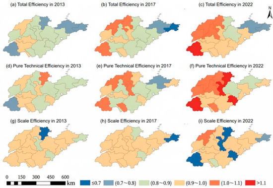
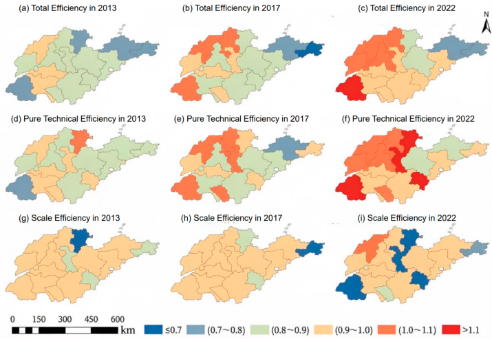
To visualize the spatial heterogeneity, the efficiency values of 2013, 2017, and 2022 were classified into six categories using the equal-interval method and mapped using ArcGIS 10.2 (Figure 1). The spatial distribution of TE and PTE exhibited a clear gradient, decreasing from Western to Eastern Shandong. High-efficiency areas (TE > 0.9) were concentrated in western cities, such as Liaocheng, Heze, and Dezhou, while eastern coastal cities, including Yantai, Weihai, and Dongying, consistently showed lower efficiency. In contrast, the spatial pattern of SE shifted westward over time, with the proportion of cities having SE above 0.9 decreasing from 35.3% in 2013 to 29.4% in 2022. This westward concentration of grain production implies increased vulnerability and uncertainty for regional food security.
3.2.3. Hot Spot and Cold Spot Analysis
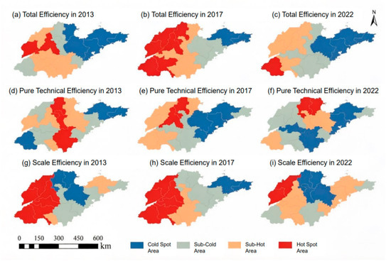
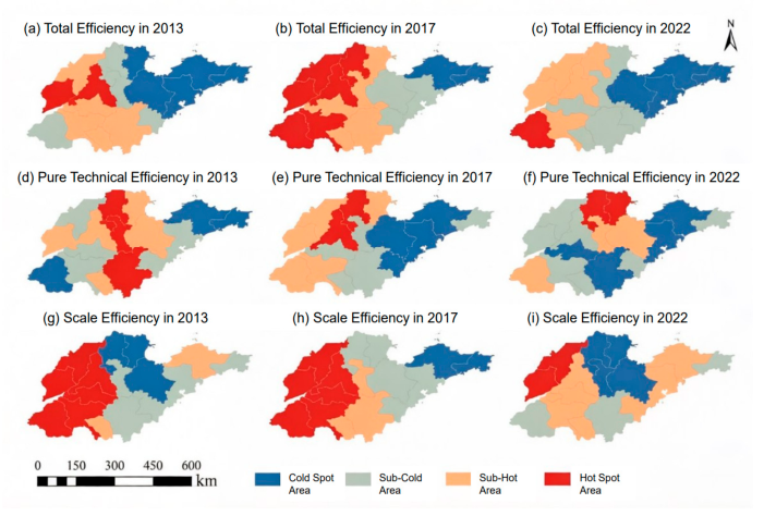
The Getis–Ord Gi* statistic was applied to identify statistically significant hot spots (high-efficiency clusters) and cold spots (low-efficiency clusters). As illustrated in Figure 3, the hot spots of TE, PTE, and SE all exhibited a westward migration trend from 2013 to 2022. The core hot spot area was consistently located in western cities, particularly Liaocheng, Heze, and Dezhou, whereas cold spots were mainly found in the eastern coastal region. The spatial extent of cold spots gradually shrank over time, but the clustering pattern became more random in the east. As illustrated in Figure 4, these findings suggest that neighboring efficiency levels exert significant spatial spillover effects: cities adjacent to high-efficiency areas are more likely to improve their own efficiency, while those near low-efficiency areas face a higher risk of decline.
Figure 3.
Scatter plot of Moran’s I in various years of grain production efficiency in Shandong Province.
Figure 4.
Distribution of cold–hot spots of grain production efficiency in Shandong Province.
3.3. Influencing Factors of Grain Production Efficiency
3.3.1. Model Construction
Based on the spatial interaction effect characteristics of grain production efficiency, traditional regression models have limitations in applicability and require the introduction of a spatial econometric framework to construct an analysis system. This research paradigm has important decision-making reference value for optimizing the layout of grain production in Shandong Province and promoting industrial quality and efficiency improvement. The spatial panel model has become the core methodological tool in this study due to its technical advantages in characterizing spatial dependencies, enhancing data parsing capabilities, and deepening spatial heterogeneity identification. The construction of its basic model follows the following paradigm.
3.3.2. Variable Selection
Based on the theoretical framework of resource endowment, efficiency evaluation, and regional spatial structure, as well as following the existing literature [38,39], eight explanatory variables were selected from four dimensions: technological progress, resource input, socioeconomic development, and infrastructure. The dependent variable is the total factor productivity change index (TFPCH) of grain production for each prefecture-level city from 2013 to 2022, as measured by the DEA–Malmquist index. Table 8 summarizes the variable definitions, units, and expected signs.
Table 8.
Variable system for influencing factors of grain production efficiency. “—” indicates no expected sign; “+” denotes an expected positive effect, and “−” denotes an expected negative effect.
Special clarification is provided for the two fertilizer indicators adopted in different model stages to avoid potential logical confusion. The total pure fertilizer amount serves as an absolute aggregate input indicator within the SBM production frontier system, which describes the overall chemical resource consumption of each city and participates in calculating green grain TFP. In contrast, fertilizer–pesticide intensity (Ferpes) is a normalized relative index measured by chemical inputs per unit cultivated land, used as an explanatory variable to interpret cross-city differences in production patterns. Furthermore, this two-stage variable framework has become a standard design in the existing agricultural efficiency literature, and is widely used by scholars, such as Wang and Long [28].
3.3.3. Robustness Test
To verify the reliability and robustness of the benchmark Spatial Durbin model results, we incorporated the geographic inverse distance matrix as a weight matrix into the model. The results are shown in Table 9.
Table 9.
Effect decomposition of panel data from the spatial Durbin model based on geographic inverse distance matrix space.
As shown in Table 9, although the spatial weight matrix is replaced from the traditional 0–1 queen adjacency matrix to the geographic inverse distance matrix, the direction and significance level of the effects of each influencing factor do not undergo fundamental changes, which further verifies the robustness and reliability of the empirical results in this study.
4. Discussion
4.1. Interpretation of Key Findings
During 2013–2022, grain production efficiency in Shandong generally improved with remarkable regional disparities. In terms of average efficiency indicators, overall technical efficiency increased from 0.8455 to 0.9605, pure technical efficiency grew from 0.9120 to 1.3310, while average scale efficiency decreased from 0.9314 to 0.8502 over the study period, showing a divergent evolutionary pattern between technical and scale dimensions. At the same time, the spatiotemporal evolution of grain production efficiency in Shandong Province is distinct. From a temporal perspective, grain production efficiency in Shandong Province fluctuates in response to technological progress and policy adjustments. For example, during the 2017–2018 crop year, Shandong Province’s grain production efficiency (TFPCH) reached 1.0486, indicating a high level of production efficiency. However, in certain years, such as the 2018–2019 crop year, efficiency declined despite significant technological progress.
The static efficiency analysis revealed significant regional disparities. Cities such as Jinan, Dezhou, Binzhou, and Heze consistently achieved high efficiency scores, whereas Weihai and Dongying lagged behind. These differences reflect heterogeneity in natural endowments, irrigation infrastructure, labor quality, and mechanization levels. For instance, the western plain areas benefit from flat terrain and concentrated farmland, while the eastern coastal regions face challenges, such as fragmented land and soil salinity, which constrain efficiency gains.
From a dynamic perspective, the Malmquist index decomposition showed that TFPCH averaged 0.9962 over the ten-year period, indicating a slight overall decline. However, notable fluctuations occurred: TFPCH peaked at 1.0486 in 2017–2018, driven jointly by technical progress (TECHCH = 1.0148) and efficiency change (EFFCH = 1.0303). In contrast, the 2018–2019 period saw a decline to 0.9634 despite significant technological progress (TECHCH = 1.1460), suggesting that technological gains alone are insufficient to compensate for declines in pure technical and scale efficiency. This underscores the need for balanced improvements across all efficiency components.
4.2. Spatial Patterns and Agglomeration Effects
Global Moran’s I analysis revealed significant positive spatial autocorrelation in grain production efficiency for most years, with values exceeding 0.4 in 2016 and 2017. Local spatial autocorrelation further identified distinct agglomeration patterns: high–high (H-H) clusters were consistently observed in western cities, such as Liaocheng, Dezhou, and Heze, while low–low (L-L) clusters dominated eastern cities, such as Qingdao, Weihai, and Yantai. These findings are consistent with the spatial convergence patterns identified by Liu et al. in the Huaihe River Ecological Economic Belt and by Zhang and Li in the Yellow River basin [40]. The persistence of these clusters suggests the presence of spatial spillover effects, where neighboring cities influence each other’s efficiency levels. This spatial dependency implies that policies aimed at improving efficiency should consider not only local interventions but also cross-regional coordination.
Cold and hot spot analysis further corroborated this west–east divide. Hot spots of comprehensive efficiency and pure technical efficiency gradually shifted westward during 2013–2022, reflecting the westward concentration of grain production. This spatial realignment may increase systemic vulnerability, as production becomes more geographically concentrated. The contraction of cold spots in eastern coastal areas indicates relative stagnation or decline, possibly due to urbanization-driven labor outmigration and farmland conversion.
4.3. Influencing Factors and Their Spatial Effects
The Spatial Durbin model results revealed complex and sometimes counterintuitive effects of various factors on grain production efficiency.
Mechanization (Mec) showed a significant positive direct effect (0.230, p < 0.001) and a positive albeit non-significant indirect effect (0.130), indicating that local mechanization improves local efficiency and may moderately benefit neighboring areas through technology diffusion. However, according to Peng and Zhang, Mec can lead to the environmental cost, such as greenhouse gas emissions, soil compaction, and degradation [41]. Therefore, smallholder farming systems commonly adopt total agricultural machinery power per unit cultivated area as an indicator to quantify the intensity of Mec [42]. In summary, how to incorporate the environmental costs of Mec into the assessment model warrants attention.
Fertilizer and pesticide intensity (Ferpes) had a significant negative direct effect (−0.0752, p < 0.05) and a negative total effect (−0.176, p < 0.01). This finding challenges the conventional belief that higher chemical input necessarily leads to higher output. Instead, this finding aligns with the research by Li et al., indicating that excessive application reduces marginal returns, degrades soil health, and increases in carbon emissions, consequently reducing overall efficiency [43]. This highlights the urgency of promoting green agricultural technologies and precision farming practices.
Urbanization (Urb) exerted the strongest negative effects, with direct, indirect, and total effects all significant at the 0.001 level (coefficients: −0.840, −0.838, −1.677). This implies that rapid urbanization draws labor and land away from agriculture, reducing the availability of experienced farmers and fragmenting production. These findings are consistent with those of Zhang and Zheng [44], who reported a negative relationship between urbanization and grain production efficiency in China. In addition, the study by Wang et al. also confirms that urban expansion in developing countries has a significant inhibitory effect on agricultural production [45].
Agricultural technology innovation (Rtec) demonstrated non-significant direct effects but significant negative indirect effects (−0.0694, p < 0.001). This suggests that while innovation may eventually improve efficiency, short-term adaptation costs and uneven technology adoption across regions can create negative spillovers. Young and McCarty’s study confirms that negative cross-regional spillovers can occur even when scale imbalances are corrected [46]. This complexity implies that technology promotion requires tailored extension services and capacity building, especially in less developed areas.
Digitalization (Tv) had a positive direct effect (0.00382, p < 0.01) but a negative indirect effect (−0.00995, p < 0.001). This dichotomy suggests that while digital tools (e.g., smart irrigation, remote sensing) improve local management, the digital divide may prevent neighboring regions from benefiting equally, potentially exacerbating spatial inequality. Currently, major approaches to addressing this imbalance include targeted rural digital infrastructure investment, customized communal precision machinery services, lightweight offline aggrotech tools, and integrated cross-regional agricultural data platforms for unlocking interregional technological spillovers [47].
The labor force level (lnpop) showed a significant negative indirect effect (−0.00158, p < 0.001), reflecting the inefficiencies associated with surplus rural labor. Excess labor increases production costs without corresponding output gains, consistent with Pan et al. [48], who found that labor hollowing out negatively affects grain production efficiency. Some East Asian countries also face this rural labor surplus barrier to food efficiency, and documented efficiency losses exceed those in Shandong Province [49].
4.4. Practical Implications
The findings carry several practical implications. First, the significant negative effect of fertilizer and pesticide intensity calls for stricter regulations on chemical inputs and stronger incentives for organic alternatives. At this phase, the province of Shandong has initiated pilot projects for transition in some regions [50]. The results of the study can provide data support and guidance for selecting suitable demonstration zones in Shandong. Second, the adverse impact of urbanization suggests that urban expansion plans must incorporate agricultural protection zones and support for part-time or multi-occupational farming. However, local governments confront practical barriers to demarcating suburban agricultural protection zones [51]. This study quantifies urbanization’s heterogeneous impacts on grain production efficiency, offering empirical support for optimizing suburban spatial planning. Third, spatiotemporal patterns of grain production efficiency across Shandong reveal marked interregional gaps in resource endowments, technology uptake, and operational scale. Western plains feature high efficiency and agglomeration, while fragmented, low-fertility terrain restricts productivity in eastern coastal and northern zones. Based on the research findings, the government can take into account the natural conditions of each region and adopt differentiated resource allocation plans.
4.5. Limitations and Future Research Directions
Despite its contributions, this study has several limitations. First, the analysis is based on prefecture-level aggregate data, which may mask heterogeneity at the farm or household level. Future research could incorporate micro-survey data to capture intra-regional variability. Second, the study period (2013–2022) does not fully capture post-pandemic recovery or recent climate extremes. Extending the time horizon would enrich the understanding of long-term dynamics. Third, while this study included carbon emissions as a non-expected output, other environmental indicators such as water footprint or biodiversity loss were not considered. Future studies could adopt more comprehensive ecological efficiency frameworks. Fourth, the spatial weight matrix used was primarily based on geographic adjacency; alternative matrices based on economic distance or information flow could yield additional insights. Finally, causal mechanisms underlying complex effects—such as the negative indirect effect of digitalization—warrant in-depth qualitative or mixed-methods investigation.
5. Conclusions
From 2013 to 2022, grain production efficiency in Shandong Province exhibited a general upward trend, yet with pronounced regional disparities. The average technical efficiency increased from 0.8455 to 0.9605, driven primarily by improvements in pure technical efficiency (0.9120 to 1.3310), while scale efficiency declined from 0.9314 to 0.8502, indicating that efficiency gains relied more on technological advancement than on scale expansion. Cities such as Jinan, Dezhou, Binzhou, and Heze achieved high efficiency levels, whereas Weihai and Dongying lagged behind. Spatiotemporally, comprehensive technical efficiency and pure technical efficiency decreased gradually from Western to Eastern Shandong, and scale efficiency became increasingly concentrated in the west, reflecting a westward shift in the grain production center. Significant spatial autocorrelation and agglomeration effects were identified, with high–high clusters in Liaocheng and Dezhou and low–low clusters in Qingdao and Weihai, confirming that spatial spillovers play an important role. Mechanization had a positive and significant direct effect on efficiency, whereas fertilizer and pesticide intensity, labor surplus, and urbanization exerted significant negative effects. Digitalization showed positive direct but negative indirect effects, implying a digital divide across regions. These findings suggest that improving grain production efficiency requires optimizing resource allocation, reducing excessive chemical inputs and labor redundancies, promoting regionally adapted technological innovation, mitigating adverse urbanization effects, and strengthening inter-city coordination to leverage positive spatial spillovers. This research adopts the DEA–Malmquist index with agricultural carbon emissions incorporated as undesirable outputs to measure and decompose total factor productivity (TFP) of grain production systems, distinguishing the contributions of pure technical efficiency and scale efficiency. Global Moran’s I is further applied to evaluate and identify spatial autocorrelation and agglomeration patterns of efficiency distribution. On this basis, the spatial Durbin model is utilized to quantitatively decompose the local direct effects, cross-regional indirect spatial spillover effects and aggregate total effects of influencing factors. Combined with spatiotemporal characteristic analysis, the multi-model framework systematically reveals the evolutionary logic of agricultural production efficiency, thereby furnishing a rigorous quantitative foundation for designing differentiated regional agricultural policies.
That said, several caveats should be acknowledged. The empirical analysis relies on prefecture-level aggregate data, which may obscure finer heterogeneity at the farm or household level; future work would benefit from micro-survey data. The study period ends in 2022 and thus misses post-pandemic recovery and recent extreme climate events; extending the time window could offer a richer understanding of long-term dynamics. While carbon emissions were included as an undesirable output, other environmental dimensions—such as water footprint or biodiversity—remain unaccounted for, pointing toward the need for more comprehensive ecological efficiency frameworks. The spatial weight matrix is also primarily based on geographic adjacency; alternative specifications using economic distance or information flow might yield additional insights. Finally, the causal mechanisms behind some complex effects, notably the negative indirect effect of digitalization, warrant further in-depth qualitative or mixed-methods investigation.
Author Contributions
Conceptualization, Y.S. and B.J.; methodology, Y.S.; software, Y.S.; validation, Y.S. and B.J.; formal analysis, Y.S.; investigation, Y.S.; resources, B.J.; data curation, Y.S.; writing—original draft preparation, Y.S.; writing—review and editing, B.J.; visualization, Y.S.; supervision, B.J.; project administration, B.J.; funding acquisition, B.J. All authors have read and agreed to the published version of the manuscript.
Funding
This research was supported by the Key Tackling Project of Shaanxi Provincial Teaching Reform Project (Shaanxi Provincial Department of Education): Construction and Practice of the Micro-Major of Agricultural Spatial Information Technology—grant number 25BG027.
Institutional Review Board Statement
This study did not require ethical approval.
Data Availability Statement
The data presented in this study are available on request from the corresponding author.
Acknowledgments
The authors sincerely thank the anonymous reviewers and editorial staff for their valuable comments and constructive suggestions, which have greatly improved the quality of this paper. We also appreciate the relevant statistical departments for providing publicly available statistical yearbooks and municipal statistical bulletins, which offered reliable data support for this research. In addition, we are grateful to our classmates and teachers for their academic communication and helpful advice during the study. Finally, we would like to express our heartfelt gratitude to our family for their constant understanding and support throughout the research process.
Conflicts of Interest
The authors declare no conflicts of interest.
Abbreviations
The following abbreviations are used in this manuscript:
| DEA | Data Envelopment Analysis |
| SBM | Slacks-Based Measure |
| CCR | Charnes–Cooper–Rhodes (model) |
| BCC | Banker–Charnes–Cooper (model) |
| DMU | Decision Making Unit |
| TE | Technical Efficiency |
| PTE | Pure Technical Efficiency |
| SE | Scale Efficiency |
| TFPCH | Total Factor Productivity Change |
| EFFCH | Technical Efficiency Change |
| TECHCH | Technological Change |
| PECH | Pure Technical Efficiency Change |
| SECH | Scale Efficiency Change |
| SFA | Stochastic Frontier Analysis |
| SDM | Spatial Durbin Model |
| SAR | Spatial Autoregressive Model |
| SEM | Spatial Error Model |
| LM | Lagrange Multiplier |
| LR | Likelihood Ratio |
| Wald | Wald Test |
| IPCC | Intergovernmental Panel on Climate Change |
| GDP | Gross Domestic Product |
| Moran’s I | Moran’s Index (global spatial autocorrelation statistic) |
| Getis–Ord Gi* | Getis–Ord Local Statistic for Hot/Cold Spot Analysis |
| H-H | High–High (spatial cluster quadrant) |
| L-L | Low–Low |
| L-H | Low–High |
| H-L | High–Low |
| Mec | Mechanization Level (variable) |
| Cult | Regional Cultural Development Level (number of rural cultural stations, variable) |
| Tv | Digitalization Level (cable TV coverage rate, variable) |
| Rtec | Agricultural Technology Innovation (patents per capita, variable) |
| Urb | Urbanization Level (urbanization rate, variable) |
| Ferpes | Fertilizer and pesticide intensity (variable) |
| lnpop | Labor Force Level (log of rural population, variable) |
| Inc | Urban–Rural Income Gap (variable) |
Appendix A
Appendix A.1
Table A1.
List of mathematical notations.
Appendix A.2
Table A2.
Descriptive statistics of input–output variables for grain production in Shandong Province.
References
- Luchtenbelt, H.; Doelman, J.; Bos, A.; Daioglou, V.; Jägermeyr, J.; Mueller, C.; Stehfest, E.; van Vuuren, D. Quantifying Food Security and Mitigation Risks Consequential to Climate Change Impacts on Crop Yields. Environ. Res. Lett. 2025, 20, 014001. [Google Scholar]
- Yang, R.; Zhou, Q.; Xu, L.; Zhang, Y.; Wei, T. Forecasting the Total Output Value of Agriculture, Forestry, Animal Husbandry, and Fishery in Various Provinces of China via NPP-VIIRS Nighttime Light Data. Appl. Sci. 2024, 14, 8752. [Google Scholar] [CrossRef] [Scilit]
- Farrell, M.J. The Measurement of Productive Efficiency. J. R. Stat. Soc. 1957, 120, 253–281. [Google Scholar] [CrossRef] [Scilit] [PubMed]
- Leibenstein, H. Allocative Efficiency vs. X-efficiency. Am. Econ. Rev. 1966, 56, 392–416. [Google Scholar]
- Cobb, C.W.; Douglas, P.H. A Theory of Production. Am. Econ. Rev. 1928, 18, 139–165. [Google Scholar]
- Coelli, T.J. A Guide to FRONTIER Version 4.1: A Computer Program for Stochastic Frontier Production and Cost Function Estimation; CEPA Working Papers; CEPA: Washington, DC, USA, 1996. [Google Scholar]
- Liu, C.M.; Fan, G.Y.; Mao, G.X.; He, P.R. Spatio-temporal Changes in Grain Production Efficiency and Influencing Factors in the Huai River Ecological and Economic Belt Over the Past Two Decades. J. Nat. Resour. 2023, 38, 707–720. [Google Scholar] [CrossRef] [Scilit]
- Wang, W.; Hu, Y.; Wang, J.; Niu, S. Urban construction land allocation efficiency of urban agglomerations in China based on a stochastic frontier production function approach. J. Clean. Prod. 2024, 434, 139965. [Google Scholar] [CrossRef] [Scilit]
- Liu, F.; Gu, L.; Liao, C.; Xue, W. Do Agricultural Production Services Improve Farmers’ Grain Production Efficiency?—Empirical Evidence from China. Sustainability 2025, 17, 6054. [Google Scholar] [CrossRef] [Scilit]
- Yin, C.J.; Yang, K.; Kong, F. Climate Change-adjusted Re-measurement of China’s Grain Total Factor Productivity. J. Huazhong Agric. Univ. (Soc. Sci. Ed.) 2025, 3, 38–52. [Google Scholar]
- Zhang, J.Y.; Jia, Q. Analysis of Grain Production Efficiency in China’s Five Major Grain-Producing Provinces Based on the DEA-Malmquist Index Model. Cent. Agric. Sci. Technol. 2024, 45, 156–161. [Google Scholar]
- Li, X.; Li, J.; Shi, X.; Shi, W. Spatially explicit assessment of crop production, nitrogen use efficiency, and environmental footprint in Iran. Agriculture 2026, 16, 851. [Google Scholar] [CrossRef] [Scilit]
- Frei, J.; Wiesenberg, G.; Hirte, J. The Impact of Climate and Potassium Nutrition on Crop Yields: Insights From a 30-year Swiss Long-term Fertilization Experiment. Agric. Ecosyst. Environ. 2024, 372, 109100. [Google Scholar] [CrossRef] [Scilit]
- Jin, H.; Han, C. Significant Increase in Eco-efficiency of China’s Grain Production From 2000 to 2022: Trend Changes, Typological Evolution, and Driving Factors. PLoS ONE 2025, 20, e0332740. [Google Scholar] [CrossRef] [Scilit] [PubMed]
- Shao, Y.; Yang, R.; An, Y. Spatial Evolution of China’s Grain Production and Its Influencing Factors. Trans. Chin. Soc. Agric. Eng. 2025, 41, 265–277. [Google Scholar]
- Liu, C.M.; Fan, G.Y.; Mao, G.X.; He, P.R. Spatio-temporal variation and influencing factors of grain production efficiency in Huaihe Eco-Economic Belt in recent 20 years. J. Nat. Resour. 2023, 38, 707–720. [Google Scholar] [CrossRef] [Scilit]
- Yu, H.; Qubi, W.; Luo, J. Digital Transformation in Agricultural Supply Chains Enhances Green Productivity: Evidence From Provincial Data in China. Earth’s Future 2025, 13, e2025EF006089. [Google Scholar] [CrossRef] [Scilit]
- Ordóñez, R.; Casteel, S.; Stevens, R.; Archontoulis, S.; Vyn, T. Climate, Rotation, and Tillage Impacts on Soybean Yield Gains in a 50-Year Experiment. Glob. Change Biol. 2025, 31, e70469. [Google Scholar] [CrossRef] [Scilit] [PubMed]
- Dong, W.; Zhang, Y.; Danso, F.; Zhang, J.; Tang, A.; Liu, Y.; Liu, K.; Meng, Y.; Wang, L.; Yang, Z.; et al. Nitrogen Fertiliser Reduction at Different Rice Growth Stages and Increased Density Improve Rice Yield and Quality in Northeast China. Agriculture 2025, 15, 892. [Google Scholar] [CrossRef] [Scilit]
- Zhang, H.; Qin, Y.; Xu, J.; Ren, W. Analysis of the Evolution Characteristics and Impact Factors of Green Production Efficiency of Grain in China. Land 2023, 12, 852. [Google Scholar] [CrossRef] [Scilit]
- Luo, J.; Huang, M.; Hu, M.; Bai, Y. How Does Agricultural Production Agglomeration Affect Green Total Factor Productivity? Empirical Evidence from China. Environ. Sci. Pollut. Res. 2023, 30, 67865–67879. [Google Scholar] [CrossRef] [Scilit] [PubMed]
- Wei, S.; Lu, Y. Adoption Mode of Agricultural Machinery and Food Productivity: Evidence From China. Front. Sustain. Food Syst. 2024, 7, 1257918. [Google Scholar] [CrossRef] [Scilit]
- Deng, Y.Y.; Zhu, J.F. Promotion Effects of Conservation Tillage Technology on Grain Production Efficiency and Environmental Efficiency. China Popul. Resour. Environ. 2023, 33, 218–228. [Google Scholar]
- Zhang, X.Y.; Wang, F.X.; Bai, L.H.; Yin, F.; Li, S.H.; Liu, L.C.; Yang, P. Study on Grain Production Efficiency and Food Security Countermeasures in Shandong Province. Shandong Agric. Sci. 2023, 55, 155–162. [Google Scholar]
- Ding, F.; Liu, C.; Wang, Y. Analysis of Grain Production Efficiency Differences in China Based on DEA-Malmquist Index. In ICMSEM 2023; Atlantis Press: Dordrecht, The Netherlands, 2023; pp. 1020–1027. [Google Scholar]
- Li, L.; Cui, M. Evaluation and Influencing Factors of Wheat Production Efficiency in Shandong Province. Agric. Eng. 2024, 14, 155–160. [Google Scholar]
- Liu, L.; Zheng, B.; Zhao, J.; Hao, S. Measurement and spatial evolution of green total factor productivity in China’s wheat production based on the three-stage DEA-GML model. Front. Sustain. Food Syst. 2025, 9, 1615861. [Google Scholar] [CrossRef] [Scilit]
- Wang, J.; Long, F. Grain industrial agglomeration and grain green total factor productivity in China: A dynamic spatial durbin econometric analysis. Heliyon 2024, 10, e26761. [Google Scholar] [CrossRef] [Scilit] [PubMed]
- Qin, T.; Zhi, Y.L.; Tong, J.P.; Wang, Z.Q. Endogenous Growth Potential and Improvement Path of China’s Grain Production Efficiency. Stat. Decis. 2024, 40, 35–39. [Google Scholar]
- Huang, F.H.; Li, X.C.; Zhang, Y.; Bi, H.W. Empirical Analysis of Grain Production Efficiency and Maize Producer Efficiency in Heilongjiang Province. J. Maize Sci. 2022, 30, 184–190. [Google Scholar]
- Liu, J.W.; Li, X.F.; Gao, P.H.; Wang, F.S. Study on Agricultural Production Efficiency and Influencing Factors in Hebei Province Based on DEA Model. J. Northeast Agric. Sci. 2020, 45, 86–91+107. [Google Scholar]
- Zhou, J.W. Analysis on Scale Effect of Regional Economic Disparities in China; CSSP: Washington, DC, USA, 2017. [Google Scholar]
- Zhang, H.; Liu, C. Compound Shocks of Pandemic Aftershocks and Meteorological Disasters on Wheat Production in Shandong Province. Front. Sustain. Food Syst. 2024, 9, 1673265. [Google Scholar]
- Charnes, A.; Cooper, W.W.; Rhodes, E. Measuring the Efficiency of Decision Making Units. Eur. J. Oper. Res. 1978, 2, 429–444. [Google Scholar] [CrossRef] [Scilit]
- Tone, K. A Slacks-based Measure of Efficiency in Data Envelopment Analysis. Eur. J. Oper. Res. 2001, 130, 498–509. [Google Scholar] [CrossRef] [Scilit]
- Malmquist, S. Index Numbers and Indifference Surfaces. Trab. Estad. 1953, 4, 209–242. [Google Scholar] [CrossRef] [Scilit]
- Färe, R.; Grosskopf, S.; Norris, M.; Zhang, Z. Productivity Growth, Technical Progress, and Efficiency Change in Industrialized Countries. Am. Econ. Rev. 1994, 84, 66–83. [Google Scholar]
- Du, L.; Wang, F.; Tian, M.; Zhao, Z.; Ma, S.; Wang, F. Spatiotemporal Differentiation and Spatial Correlation of Agricultural Total Factor Productivity in China: An Estimation Based on the Data of Prefecture-level Cities. Cienc. Rural 2023, 53, e20210877. [Google Scholar] [CrossRef] [Scilit]
- Shen, L.; Sun, R.; Liu, W. Examining the Drivers of Grain Production Efficiency for Achieving Energy Transition in China. Environ. Impact Assess. Rev. 2024, 105, 107–121. [Google Scholar] [CrossRef] [Scilit]
- Zhang, L.; Li, R. Research on Agricultural Machinery Service Development and Grain Production Efficiency (2004–2016): Based on Stochastic Frontier Analysis of Variable Coefficient. J. Huazhong Agric. Univ. (Soc. Sci. Ed.) 2020, 67–77. [Google Scholar]
- Peng, C.; Zhang, C. Impact of Agricultural Mechanization on Farmers’ Grain Production Efficiency. J. South China Agric. Univ. (Soc. Sci. Ed.) 2020, 19, 93–102. [Google Scholar]
- Food and Agriculture Organization. Agricultural Mechanization and Sustainable Agrifood System Transformation in the Global South; Food and Agriculture Organization: Rome, Italy, 2022. [Google Scholar]
- Li, Q.; Zhai, Q.; Wang, X.; Wang, J. The Dual Impacts of Specialized Agricultural Services on Fertilizer Application Intensity. Food Energy Secur. 2025, 14, e70153. [Google Scholar] [CrossRef] [Scilit]
- Zhang, L.; Zheng, X.G. VAR Model Analysis on the Relationship Between Urbanization and Grain Production Efficiency. Chin. J. Agric. Resour. Reg. Plan. 2017, 38, 96–100. [Google Scholar]
- Wang, S.; Zhang, X.; Deng, O.; Gu, B. Interplay of urbanization and agricultural modernization shapes nitrogen use in global croplands. Nat. Commun. 2026, 17, 3128. [Google Scholar] [CrossRef] [Scilit] [PubMed]
- Young, J.S.; McCarty, T.; Lancaster, S.; Bish, M. Modeling Soybean Planting Decisions with Network Diffusion: Does Herbicide Drift Affect Farmer Profitability and Seed Selection? J. Agric. Appl. Econ. 2023, 55, 304–323. [Google Scholar] [CrossRef] [Scilit]
- McFadden, J. The digitalisation of agriculture: A literature review and emerging policy issues. In OECD Food, Agriculture and Fisheries Papers; OECD: Paris, France, 2022. [Google Scholar]
- Pan, G.Y.; Chen, W.J.; Xiong, L.B. Rural Labor Hollowing, Planting Structure and Grain Production Efficiency. J. Neijiang Norm. Univ. 2025, 40, 67–75. [Google Scholar]
- Ayerst, S.; Brandt, L.; Restuccia, D. Market constraints, misallocation, and productivity in Vietnam agriculture. Food Policy 2020, 94, 101840. [Google Scholar] [CrossRef] [Scilit]
- Wang, Q.X. Integrated agrochemical reduction demonstration system for open-field vegetable production in Anqiu City. Plant Prot. 2025, 51, 132–139. [Google Scholar]
- Bo, L.M.; Yin, L.; Zhao, L. Evolution characteristics and driving factors of territorial spatial pattern in Shandong Province from the perspective of major functional zoning. Geogr. Geo-Inf. Sci. 2024, 40, 62–70. [Google Scholar]

Disclaimer/Publisher’s Note: The statements, opinions and data contained in all publications are solely those of the individual author(s) and contributor(s) and not of MDPI and/or the editor(s). MDPI and/or the editor(s) disclaim responsibility for any injury to people or property resulting from any ideas, methods, instructions or products referred to in the content. |
© 2026 by the authors. Licensee MDPI, Basel, Switzerland. This article is an open access article distributed under the terms and conditions of the Creative Commons Attribution (CC BY) license.