Nonlinear Threshold Effects of Agricultural Inputs on Crop Production in China: Insights from XGBoost-SHAP and Spatiotemporal Analysis

Abstract

Understanding the spatiotemporal relationship between agricultural inputs and crop production is essential for sustainable agricultural management. Using provincial panel data from China from 2000 to 2022, this study integrates spatiotemporal analysis with the XGBoost-SHAP model to examine the nonlinear effects of agricultural machinery, fertilizers, pesticides, and plastic films on soybean, cereal, and tuber yields. The results show that China’s agricultural input system shifted around 2015 from input-intensive growth toward green transformation, with fertilizer, pesticide, and plastic-film use declining after this inflection point. Spatially, agricultural inputs and crop production show clear agglomeration and path dependence: machinery is concentrated in northern China, fertilizers and pesticides in eastern intensive farming regions, and plastic-film use in arid and cold regions, while soybean, cereal, and tuber production are mainly concentrated in Northeast China, the Northeast-Huang-Huai-Hai region, and Southwest China, respectively. The SHAP results reveal distinct crop-specific importance rankings and nonlinear threshold patterns. For soybean yield prediction, agricultural plastic film use contributes most strongly to the model output, followed by fertilizer application, pesticide use, and machinery power; its SHAP contribution turns negative beyond approximately 112.4 thousand tons. For cereal yield prediction, machinery power ranks first, followed by fertilizer application, pesticide use, and plastic-film use; its contribution becomes positive beyond approximately 28.34 million kW and then gradually levels off. For tuber yield prediction, fertilizer application is the dominant predictor, followed by pesticide use, machinery power, and plastic-film use; its contribution turns negative beyond approximately 1.35 million tons. These findings indicate that agricultural inputs have crop-specific nonlinear effects, and that input regulation should prioritize the most influential factors for each crop while considering their threshold ranges. The study provides a scientific basis for differentiated, crop-specific, and regionally adaptive agricultural input management.

1. Introduction

Amid rising food security pressures, with the global population projected to reach approximately 9.7 billion by 2050, agricultural systems face major challenges. The Green Revolution, defined by synthetic chemicals and mechanization, has increased global food production but strained natural resources and ecosystems [1,2]. China, as the largest food producer and consumer, sustains nearly 20 percent of the global population on less than 9% of the world’s arable land. This relies on intensive inputs, including machinery, fertilizers, pesticides, and plastics [3,4,5]. Nevertheless, the environmental consequences include soil degradation, water pollution, and biodiversity loss, threatening the sustainability of agricultural ecosystems [6,7,8,9]. Accordingly, reassessing and quantifying the relationship between agricultural inputs and outputs is essential for optimizing yields while reducing environmental impacts under resource constraints. This supports China’s strategies of increasing crop production through soil conservation and technology and provides a model for sustainable global food production.

Modern agricultural productivity depends on managing external material inputs. A key question is whether the input-yield relationship is linear or nonlinear, with potential thresholds where benefits plateau or decline. Traditionally, studies assume that higher inputs directly increase yields, adopting linear response models [10,11]. In contrast, empirical evidence and ecological theory indicate that agricultural ecosystems exhibit nonlinear dynamics [12,13,14]. A classic theory in agricultural economics—the law of diminishing marginal returns—provides an important theoretical explanation for this nonlinear relationship. This law states that, provided the level of technology and other inputs remain constant, if the input of a particular variable factor is increased by the same amount repeatedly, its marginal product will eventually begin to decline; once the input exceeds a certain critical threshold, the marginal product may even fall to zero or become negative. For instance, nitrogen fertilizer beyond crop absorption capacity reduces marginal yields and generates externalities such as greenhouse gas emissions and eutrophication [7,15]. Excessive pesticide use promotes pest resistance and disrupts natural enemies, potentially leading to increased outbreaks [16,17,18]. Similar patterns apply to machinery and plastic films, influenced by soil, tillage, and climate factors. These nonlinear features, along with interactions among inputs, limit the utility of linear models for precision agriculture [13]. Identifying and quantifying nonlinear response curves and inflection points is thus essential for reducing inputs, enhancing efficiency, and advancing sustainable practices.

Previous studies have examined crop yield responses to climatic, technological, and management factors, as well as input-output linkages in agricultural production systems [19,20,21] and provide estimates of their output elasticity [21]. Some studies have also identified nonlinear effects and spatial heterogeneity by incorporating quadratic terms or employing spatial econometric models. However, these methods have inherent limitations. Traditional econometric models depend on predetermined functional forms, often failing to accurately capture the complex, high-dimensional, and irregular relationships between inputs and outputs in real-world agriculture [21]. In recent years, machine learning methods have become powerful tools for predicting agricultural yields and analyzing input-output relationships.

Research indicates that Random Forests (RF), Artificial Neural Networks (ANN), Support Vector Machines (SVM), and XGBoost are the most widely used machine learning algorithms in crop yield forecasting. Meanwhile, Long Short-Term Memory (LSTM) and Convolutional Neural Networks (CNN) are commonly employed for capturing temporal and spatial characteristics of agricultural systems [22]. In particular, RF demonstrates strong generalization capabilities and robustness to outliers in high-dimensional data through its ensemble strategy of randomized decision trees, making it suitable for exploratory yield forecasting studies [23]. ANNs possess strong nonlinear fitting capabilities, but are typically suited to large-scale training datasets to avoid overfitting [24]. SVM uses kernel functions to map low-dimensional nonlinear relationships onto a high-dimensional linearly separable space, offering advantages in applications involving small sample sizes and high-dimensional regression problems [23]. LSTMs are particularly effective at capturing long-term dependencies in time series and are frequently used for forecasting seasonal crop yields [22]. CNN is capable of extracting spatial features from rasterized data such as remote sensing imagery, enabling large-scale yield estimation [25].

Among the methods mentioned above, XGBoost offers particular advantages when analyzing small- to medium-scale agricultural datasets. Firstly, its built-in L1 and L2 regularization mechanisms provide effective control over overfitting in small- to medium-scale datasets (this advantage is particularly crucial given the sample size constraints of agricultural panel data, whereas deep learning methods such as LSTM carry a significant risk of overfitting on small datasets) [22]. Secondly, unlike traditional parametric models that require predefined functional forms, XGBoost is able to automatically learn complex high-dimensional nonlinear relationships and variable interactions directly from the data through a gradient boosting ensemble framework. It can also efficiently handle missing values and mixed data types, thereby reducing the burden of data preprocessing [26]. Despite the strong predictive performance of machine learning algorithms, their ‘black box’ nature limits their interpretability. This lack of transparency weakens their usefulness for agricultural decision-making. More importantly, most existing studies treat food as a homogeneous entity [19,27], focusing either on total production analysis or on specific crop categories [28], neglecting differences among crop types such as soybeans, cereals and tubers in response to inputs and the comparative analysis of their characteristics. However, soybeans, cereals and tubers differ significantly in terms of their physiological characteristics, cultivation methods and dependence on inputs. This oversight obscures key structural details, limiting their precision and applicability.

To address these limitations, this study develops an analytical framework that integrates spatial analysis with interpretable machine learning. It aims to elucidate the nonlinear impacts of agricultural material use on different crop yields. We have introduced the SHAP interpretability framework. This feature attribution method, based on cooperative game theory, provides consistent and locally additive explanations for each prediction. In recent years, when combined with dependence plots and smoothing methods, SHAP has helped identify model-based turning points in feature contributions—specifically, the critical points at which the direction of the effect changes and the effect intensity undergoes a qualitative change; its effectiveness in this regard has been thoroughly validated [29,30,31,32]. Consequently, drawing on the data structure characteristics of this study and building upon the use of XGBoost to investigate the relationship between agricultural inputs and crop yields, we employ SHAP dependency graphs to reveal how the marginal contribution of each agricultural input changes as input levels vary and to identify the critical turning points at which effects shift from positive to negative, as well as the inflection points where marginal returns tend toward saturation. This interpretability is crucial for translating model predictions into actionable policy recommendations.

We focus on three core research objectives: (1) Within a spatiotemporal framework, revealing the spatiotemporal patterns and spatial heterogeneity of China’s major agricultural inputs and the yields of soybeans, cereals and tubers between 2000 and 2022; (2) identifying the nonlinear impact patterns of four key agricultural inputs (total agricultural machinery power, chemical fertilizers, pesticides and agricultural plastic film) on the yields of various crops, along with the characteristics of their critical input thresholds; (3) taking into account crop-specific threshold response characteristics and regional differences in resource endowments, proposing precision agriculture management strategies based on zoning, classification and grading. Achieving these research objectives will establish a vital scientific foundation to overcome the high input-high output dilemma and promote a transition from experience-based policies to data-driven, precision agricultural management.

This study employs spatial pattern analysis using GIS and introduces the XGBoost model in conjunction with the SHAP framework for an in-depth analysis of China’s provincial panel data. The core innovations of this study are as follows: (1) The integration of GIS + XGBoost-SHAP, advancing the transition from correlation inference and black-box prediction to nonlinear attribution. This framework provides a robust tool for analyzing complex agricultural systems. (2) A classification-based analysis of soybeans, cereals and tubers, uncovering crop-specific response patterns previously obscured. These findings support the development of targeted agricultural input management policies. This research is expected to serve as a scientific reference for countries and regions facing similar challenges, supporting efforts to balance food security with sustainable agricultural development.

2. Materials and Methods

2.1. Materials

2.1.1. Variable Selection

To systematically assess the impact of agricultural material consumption on food production, this study establishes a comprehensive variable system, as presented in

Table 1. Definition and explanation of variables.

Variable Category	Variable Name	Variable Abbreviation	Unit
Dependent Variables	Soybean Yield	SY	104 t
	Cereal Yield	CY	104 t
	Tuber Yield	TY	104 t
Core Independent Variables	Total Power of Agricultural Machinery [33]	AMP	104 kW
	Agricultural Chemical Fertilizer Application Amount [34]	AFA	104 t
	Pesticide Usage [35]	PU	104 t
	Agricultural Plastic Film Usage [36]	AFU	104 t
Control Variables	Added Value of Primary Industry	AVPI	108 CNY
	Rural Population	RP	104 persons
	Crop Sown Area	CSA	kha

. The reasons for selecting soybean yield (SY), cereal yield (CY) and tuber yield (TY) as the primary output indicators in this study are as follows: (1) According to the statistical definition used by the National Bureau of Statistics of China, grain crops cover cereals, beans, and tubers, which together form the core framework of China’s food security. In particular, soybeans are a fundamental and strategic agricultural product that is vital to the national economy and people’s livelihoods; they are both a food crop and an oilseed crop, and are a prime example of legumes. (2) There are significant differences between the three crop types in terms of growth characteristics, cultivation methods and input dependency. In terms of nutrient requirements, leguminous crops such as soybeans are significantly less dependent on chemical nitrogen fertilizers due to nitrogen fixation by rhizobia, but have a particular preference for phosphorus fertilizers; cereals do not fix nitrogen and are highly dependent on external nitrogen fertilizers; tubers have the highest potassium requirements of all crops and are extremely sensitive to imbalances in nutrient ratios. In terms of suitability for mechanization, cereals are best suited to large-scale mechanical operations, followed by soybeans; tubers, however, are the most susceptible to mechanical damage due to the fragility of their underground parts. In terms of nitrogen utilization mechanisms, these three plants belong to the Fabaceae, Poaceae and Solanaceae/Convolvulaceae families, respectively representing three distinct input-response pattern prototypes. (3) The data for these three crop types are readily available and nationally representative; as these crops are cultivated and yield statistics are recorded across all 31 provinces, they provide a solid basis for panel data analysis at the national level. This classification facilitates a nuanced understanding of the differential impacts of agricultural inputs on various components within China’s food production system, thereby extending beyond a general analysis of total food output.

The independent variables of this study focus on four material inputs that are decisive for modern agricultural production. Specifically, these variables include: total power of agricultural machinery (AMP), which serves as an indicator of the mechanization level and equipment endowment in agricultural production. It is widely used in research on agricultural productivity and agricultural modernization [33]. Agricultural chemical fertilizer application (AFA), which represents the intensity of nutrient inputs into the soil, quantifies the extent of human intervention in agricultural ecosystem nutrient cycles [34]. Pesticide usage (PU) refers to the total amount of chemical agents applied in agricultural production and reflects the intensity of chemical pest, disease, and weed management [35]. Agricultural plastic film usage (AFU) indicates the adoption intensity and spatial extent of plastic-film mulching technology in modern agriculture [36]. These four inputs collectively constitute the key dimensions for measuring agricultural intensification in China.

To more precisely isolate the net effect of the aforementioned core materials and to mitigate potential model bias arising from omitted variables, this study further incorporates control variables spanning multiple dimensions, including the agricultural economic foundation, labor input, and land resource endowment. Among these, the added value of the primary industry serves to reflect the overall economic scale and developmental level of regional agriculture, thereby accounting for the influence of the macroeconomic environment on agricultural production. Regions with a higher level of economic development typically have better agricultural infrastructure and greater capacity to invest in agriculture. The rural population is utilized as a proxy for agricultural labor, effectively measuring the scale of potential labor input. Agriculture remains a labor-intensive industry, and the supply of labor directly influences decisions regarding production inputs. Additionally, crop sown area is included to partially control for the scale effect of land use, although the dependent variables remain total crop outputs rather than yields per unit area. It should be noted that this study did not include climatic variables (such as annual average temperature, annual precipitation and hours of sunshine) in its variable selection, primarily for the following reasons: (1) This study aims to quantify the marginal effects of human-controlled agricultural inputs on yield in order to inform policy-making; however, climatic variables are exogenous factors in agricultural production that cannot be directly influenced by farmers’ short- to medium-term decisions, and thus deviate to some extent from the objectives of this study. (2) From a methodological perspective, at the provincial panel level, there is significant spatial multicollinearity between climatic variables and agricultural inputs. For instance, provinces with high precipitation systematically reduce their application of chemical fertilizers due to increased risks of nutrient leaching, whereas provinces with high temperatures tend to have lower levels of mechanization owing to their hilly terrain. Including both types of factors simultaneously may lead to unstable coefficient estimates and obscure the identification of the net effect of controllable inputs.

2.1.2. Data Description

This study constructs a provincially balanced panel dataset covering China’s 31 provinces, autonomous regions and municipalities, covering the period from 2000 to 2022 and comprising a total of 713 province-year observations. All raw data are sourced from the China Statistical Yearbook, the China Rural Statistical Yearbook and the respective provincial statistical yearbooks. To enhance data transparency, this study reports the mean, standard deviation, minimum, maximum, VIF, tolerance and quartiles for each variable in

Table 2. Descriptive statistics for variables.

	Count	Mean	Std	Min	25%	75%	Max	VIF	Tolerance
SY	713	63.13	114.36	0.10	14.00	67.10	966.40	/	/
CY	713	1662.91	1492.38	27.70	528.60	2581.40	7104.40	/	/
TY	713	102.23	103.77	0.00	31.80	149.80	559.20	/	/
AMP	713	2833.06	2718.02	73.69	902.94	3537.06	13,353.02	5.94	0.17
AFA	713	169.24	137.65	2.50	74.80	245.26	716.10	8.48	0.12
PU	713	4.97	4.14	0.05	1.26	7.83	17.35	3.67	0.27
AFU	713	6.85	6.36	0.01	2.56	9.18	34.35	2.11	0.47
AVPI	713	1481.77	1343.39	36.32	364.50	2195.11	6298.60	2.55	0.39
RP	713	2052.64	1493.49	160.78	997.41	2977.17	7286.78	3.91	0.26
CSA	713	5200.10	3704.49	88.60	2263.10	7797.90	15,209.40	5.04	0.20

, and presents box plots for the dependent variable, key agricultural input variables and control variables in Figure S1. The VIF values range from 2.114 to 8.477, and the tolerance values range from 0.118 to 0.473, indicating that the explanatory variables do not suffer from severe multicollinearity. Given the significant differences in the units and orders of magnitude of the various variables, Figure S1 presents the data using a univariate analysis approach to avoid graphical compression caused by differences in scale. The box plots reveal marked dispersion in agricultural inputs and crop yields across different provinces, with some major agricultural provinces constituting statistically significant outliers. Following an item-by-item comparison with the original statistical yearbook, no significant data entry errors were found; consequently, this study has not mechanically excluded these observations on the basis of statistical thresholds alone. This is because these high values may reflect genuine differences between provinces in terms of the scale of arable land, the composition of major crops, and agricultural production capacity. The revised model mitigates the impact of outliers on model complexity through tree depth constraints, row-column sampling, and L1 and L2 regularization, and assesses the sensitivity of the results to changes in sample composition using provincial cluster bootstrapping.

2.1.3. Data Preprocessing

Prior to model construction, the data are first sorted by year, and the training and testing periods are defined. Missing values are then imputed and the model estimated, to ensure that information from the testing period does not influence the training process. Observations with missing values for the dependent variable are excluded from the estimation of the corresponding crop model; individual missing values for the independent variables are imputed using the median value from the training sample. Missing value imputation is embedded within the model pipeline and is fitted separately within each cross-validation fold; consequently, neither the validation nor the independent test data are used to determine the imputation parameters. XGBoost is a decision-tree-based ensemble model that is insensitive to variable scales. To preserve the original units of measurement for agricultural input variables and to facilitate the interpretation of SHAP response curves, the XGBoost model no longer performs full-sample Z-score standardization on continuous variables. In the linear, quadratic and Translog benchmark models, standardization is incorporated into the respective training pipelines, with means and standard deviations estimated using only the corresponding training samples. With the exception of data errors identified through verification of the raw data, this study does not automatically remove observations that are statistically outliers.

2.2. Methods

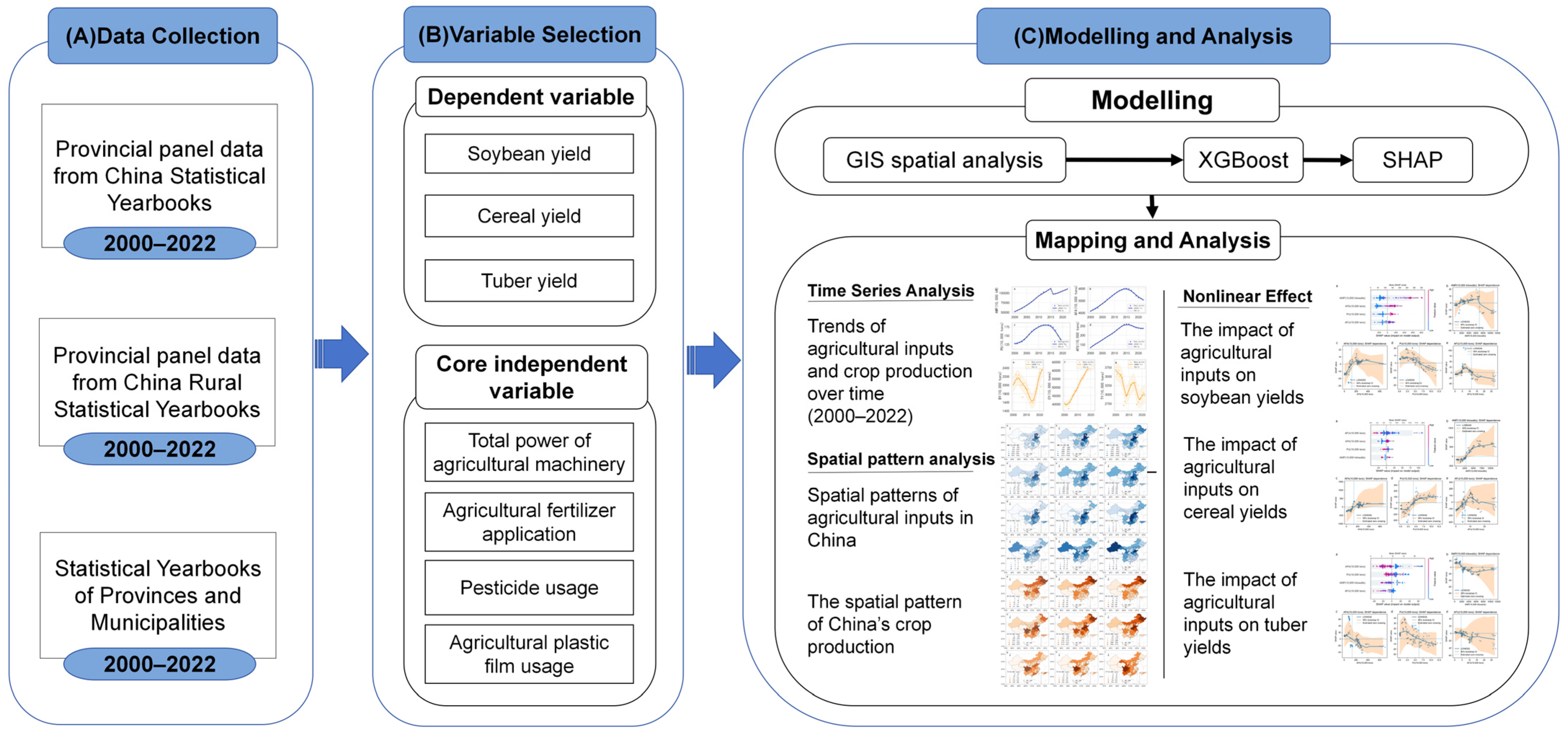
This study’s methodological framework combines GIS spatial analysis, XGBoost, and SHAP interpretability, forming a comprehensive pipeline from spatial pattern detection to nonlinear attribution. Specifically, we first use GIS to perform exploratory spatial data analysis, visually illustrating crop yield distribution across Chinese provinces with graded color thematic maps. This approach, using methods like the standard deviational ellipse, facilitates the analysis of evolution trends and spatial clustering over time. Building on previous work [31,32,37], we employ the XGBoost model to accurately capture complex, high-dimensional nonlinear relationships and interactions between various agricultural inputs (independent variables) and crop yields (dependent variables). XGBoost is an ensemble learning algorithm based on gradient-boosted decision trees. Unlike traditional parametric methods—such as the Cobb–Douglas production function—which require the form of the function to be specified in advance, XGBoost is able to automatically learn complex high-dimensional nonlinear relationships and interactions between variables directly from the data. The algorithm constructs an additive predictive model by iteratively adding weak learners (decision trees), with each new tree fitting the gradient direction of the residuals from the previous ensemble model. This model eschews reliance on predefined functional forms, enabling efficient handling of complex system dynamics and interactions. Finally, to clarify the “black box” nature of the XGBoost model, we use the SHAP method based on game theory for post hoc interpretability. This approach allows precise, transparent measurement of each input variable’s contribution to crop yield globally and locally. The complete methodological workflow is delineated in Figure 1, illustrating a systematic progression from descriptive analysis to detailed attribution.

No commercial chemicals, reagents, devices, instruments, commercial cell lines, biological samples, or other commercial experimental materials were used in this study. The agricultural input variables were province-level statistical indicators rather than manufacturer-specific products. All statistical analyses and machine-learning procedures were implemented in Python 3.11.9, using pandas 2.2.3, NumPy 1.26.4, scikit-learn 1.6.1, XGBoost 2.1.4, SHAP 0.49.1, statsmodels 0.14.6, and TensorFlow 2.18.0. Spatial maps were generated using Matplotlib 3.10.8, Cartopy 0.25.0, frykit 0.8.1, and GeoPandas 1.1.2.

2.2.1. XGBoost Model

Extreme Gradient Boosting (XGBoost) is an efficient, flexible, and scalable ensemble learning model built upon the Gradient Boosting Decision Tree (GBDT) algorithm [26]. It builds a series of weak learners iteratively, with each new tree fitting the residual errors of the combined previous trees, thereby reducing bias and improving accuracy. Compared to traditional GBDT, XGBoost includes numerous optimizations that boost efficiency and predictive power, making it one of the most robust supervised learning algorithms today. This study constructs yield prediction models for soybeans, cereals, and tubers, respectively. The explanatory variables in the models include four key agricultural inputs—total power of agricultural machinery, agricultural chemical fertilizer application amount, pesticide usage, and agricultural plastic film usage—as well as three control variables: added value of primary industry, rural population, and crop sown area. To prevent data leakage during preprocessing, median estimation for missing values has been incorporated into the model training pipeline. During each round of model training and cross-validation, imputation parameters are estimated solely on the basis of the corresponding training samples and are then applied to the validation or test samples.

Given that provincial panel data have a clear chronological sequence, randomly splitting the data into training and test sets may allow information from future years to influence the model’s parameter selection process, thereby overestimating the model’s ability to extrapolate over time. Therefore, this study adopts a time-series extrapolation validation design based on complete years. The main analysis designates the period from 2000 to 2017 as the training period and the period from 2018 to 2022 as the independent testing period, accounting for approximately 78% and 22% of the total study years, respectively. All available provincial observations from the same year are always assigned to the same data subset, thereby preventing cross-sectional information from the same period from appearing in both the training set and the test set. The test period is not included in the estimation of missing value imputation parameters or hyperparameter optimization; it is used solely for the final out-of-time extrapolation evaluation and model benchmarking.

The XGBoost hyperparameters were determined solely for the training period from 2000 to 2017. This study employs five-fold cross-validation with expanding time windows, whereby each fold uses earlier years as training data and the subsequent consecutive years as validation data, ensuring that any validation year is later than all the training years included in that fold. A random search method was employed to evaluate 60 sets of hyperparameter combinations, with the selection criterion being the minimization of cross-validation RMSE. The search parameters included the number of decision trees, learning rate, maximum tree depth, minimum child node weight, sample sampling ratio, feature sampling ratio, minimum loss decline, and L1 and L2 regularization coefficients. Once the optimal hyperparameters were obtained, the model was refitted on the complete 2000–2017 training period and evaluated via a one-time extrapolation on the 2018–2022 independent test period.

The predictive performance of the model is measured using the coefficient of determination (R²), the mean absolute error (MAE), and the root mean square error (RMSE). To diagnose overfitting, this study reports evaluation metrics for both the training and testing phases and uses the difference between the testing RMSE and the training RMSE to measure the model’s generalization gap. Training set metrics are primarily used to identify whether the model is overfitted, whereas the model’s validity is primarily assessed on the basis of its performance on the independent test set.

The uncertainty in the evaluation indicators for the trial period was estimated using provincial cluster bootstrapping. In each round, sampling with replacement was conducted using provinces as the sampling units, and all annual observations for the selected provinces during the period 2018–2022 were retained in order to preserve the temporal structure of the observations within each province. Based on 2000 repeated samples, 95% confidence intervals were constructed for the test period (R²), MAE and RMSE. These confidence intervals primarily reflect the uncertainty in predictive performance arising from changes in the composition of the provincial samples during the test period.

To compare the predictive capabilities of XGBoost with those of traditional parametric models, this study further establishes several benchmark models, including a standard linear regression model; a quadratic Ridge model comprising linear terms, quadratic terms and two-way interaction terms; a Translog Ridge model that applies logarithmic transformations to both the explanatory and response variables and introduces second-order terms; an LSTM model; and an XGBoost model using pre-set regularization parameters. All models utilize the same training and testing periods and the same set of explanatory variables. This study employs a paired provincial-cluster bootstrap test to compare the test-set RMSE of the tuned XGBoost model with those of the benchmark models to determine whether the differences in predictive performance are statistically robust.

Furthermore, to assess the sensitivity of the results to the time-period division scheme, this study conducts a robustness analysis using an approximate 70%/30% time-period division, with the period 2000–2015 serving as the training period and 2016–2022 as the testing period. The robustness analysis utilized the XGBoost hyperparameters selected in the main analysis, without re-tuning the parameters for the alternative test period, in order to avoid a secondary model selection based on the prediction results from the robustness samples.

It should be noted that this study consistently employs the tuned XGBoost model, determined via cross-validation during the training period, in the subsequent SHAP analysis. The hyperparameters of this model were established prior to evaluation on the independent test set and are not subsequently adjusted based on the relative performance of any benchmark model during the test period. The consistent use of the tuned XGBoost model not only avoids test-set-driven model selection but also facilitates the comparison of the nonlinear responses of different crops to agricultural inputs and the characteristics of variable interactions under the same model structure.

Table 3. Predictive performance of different crop models during the independent test period and 95% confidence intervals.

Crop	Model	Training R2	Training RMSE	Test (R2) (95% CI)	Test MAE (95% CI)	Test RMSE (95% CI)
Soybeans	Linear OLS	0.687	57.724	0.721 (−2.197, 0.786)	50.334 (35.210, 71.187)	77.825 (45.246, 114.268)
	Quadratic Ridge	0.864	38.019	0.933 (0.300, 0.956)	21.179 (13.727, 29.907)	38.050 (19.899, 55.086)
	Translog Ridge	0.629	62.832	0.548 (0.496, 0.775)	32.791 (11.338, 68.206)	99.010 (16.304, 167.994)
	LSTM	0.903	32.18	0.773 (0.417, 0.788)	28.713 (13.370, 53.093)	70.099 (19.342, 115.979)
	Regularized XGBoost	0.981	14.16	0.786 (0.610, 0.856)	24.176 (9.867, 45.854)	68.206 (13.916, 113.821)
	Tuned XGBoost	0.987	11.779	0.759 (0.571, 0.811)	26.641 (11.326, 50.629)	72.289 (15.834, 120.480)
Cereals	Linear OLS	0.909	410.448	0.888 (0.785, 0.933)	489.219 (370.831, 615.445)	618.171 (468.161, 758.845)
	Quadratic Ridge	0.949	307.303	0.917 (0.825, 0.957)	364.170 (266.785, 472.888)	531.270 (392.325, 665.737)
	Translog Ridge	0.926	369.412	0.912 (0.816, 0.954)	347.574 (216.744, 489.516)	549.253 (373.879, 714.347)
	LSTM	0.866	498.707	0.748 (0.640, 0.889)	540.409 (305.624, 825.710)	928.602 (443.570, 1330.574)
	Regularized XGBoost	0.990	136.728	0.942 (0.876, 0.972)	311.652 (218.341, 414.004)	445.494 (306.783, 580.010)
	Tuned XGBoost	1.00	17.581	0.958 (0.897, 0.983)	236.386 (157.259, 322.196)	378.053 (238.174, 520.194)
Tubers	Linear OLS	0.496	71.487	0.365 (−1.223, 0.661)	71.724 (53.645, 89.850)	90.594 (69.848, 108.542)
	Quadratic Ridge	0.707	54.509	0.649 (−0.239, 0.828)	53.975 (43.435, 64.633)	67.372 (55.171, 78.281)
	Translog Ridge	0.529	69.116	0.475 (−0.127, 0.606)	53.053 (32.434, 74.679)	82.350 (49.419, 110.506)
	LSTM	0.791	46.042	0.610 (−0.115, 0.753)	50.389 (33.810, 69.140)	70.997 (46.179, 92.663)
	Regularized XGBoost	0.960	20.143	0.642 (0.300, 0.771)	42.383 (28.282, 60.835)	67.986 (39.890, 99.047)
	Tuned XGBoost	0.999	2.907	0.751 (0.547, 0.858)	33.250 (22.774, 48.256)	56.756 (31.633, 84.116)

reports the predictive performance of the different models during the training period and the independent testing period from 2018 to 2022. Overall, the extrapolation capabilities of the models vary across different crops. The tuned XGBoost model achieved the highest test-set R² and the lowest MAE and RMSE for both cereals and tubers, demonstrating strong overall predictive capability; for soybean prediction, the test-set metrics of the quadratic Ridge model were numerically superior to those of the tuned XGBoost model, but the bootstrap confidence intervals for the difference in RMSE between the two included zero, which is insufficient to conclude that there is a consistent difference in their extrapolation performance.

To assess the sensitivity of the model results to the time-splitting scheme (see Table S4), this study further conducted a robustness test using a 70%/30% time extrapolation approach, with the period 2000–2015 serving as the training period and 2016–2022 as the testing period. The results show that for the soybeans model, the R² value for the test set of the tuned XGBoost model changed from 0.759 in the main analysis to 0.755, while the RMSE changed from 72.289 to 68.917, representing a minor overall change; for the cereals model, the test-set R² decreased from 0.958 to 0.934, while the RMSE increased from 378.053 to 473.267; for the tubers model, the test-set R² decreased from 0.751 to 0.709, and the RMSE increased from 56.756 to 60.395. This indicates that the conclusions of the main model comparison remain generally robust across different time horizons, but the predictive accuracy of the models is still affected by the extrapolation period.

In the cereals model, the tuned XGBoost achieved a test-set R² of 0.958, with MAE and RMSE of 236.386 and 378.053 respectively, outperforming the other models. Paired bootstrap tests further indicate that the tuned XGBoost model reduces RMSE by 243.858, 158.220, 170.605 and 529.064 compared to the linear OLS, quadratic Ridge model, the Translog Ridge model and the LSTM model, respectively, with all differences reaching statistical significance (all p ≤ 0.003). In the tubers model, the tuned XGBoost model achieved a test-set R² of 0.751 and an RMSE of 56.756; its prediction error was significantly lower than that of the linear model and the Translog Ridge model, but the advantage over the quadratic Ridge model and the LSTM model was not statistically significant (p = 0.443 and p = 0.132).

In the soybeans model, the quadratic Ridge model achieved the highest test-set R² and the lowest RMSE, at 0.933 and 38.050 respectively; the corresponding metrics for the tuned XGBoost were 0.759 and 72.289. The difference in RMSE between the tuned XGBoost and the quadratic Ridge model was not statistically significant (95% CI: −13.339 to 68.700, p = 0.391). Overall, the tuned XGBoost model performed best for cereals and tubers, while also maintaining a good ability to fit nonlinear relationships in the soybeans model. Given that its hyperparameters are determined entirely through cross-validation during the training phase, and that future research will require a comparison of SHAP contributions and nonlinear responses across different crops within a unified model framework, the subsequent analyses in this study will uniformly employ the tuned XGBoost model.

2.2.2. SHAP Model

This study uses TreeExplainer to calculate the SHAP values for the XGBoost model. To ensure consistency between the interpretation results and the prediction evaluation, the main SHAP analysis is based solely on the independent test set samples from 2018 to 2022, rather than the full dataset comprising both the training and test sets. Global feature importance is measured using the average absolute SHAP value; SHAP swarm plots are used to illustrate variable values, the direction of influence and sample heterogeneity; SHAP dependency plots are used to describe the nonlinear relationship between feature values and model contributions.

To avoid subjective interpretation of thresholds based on a single fitted curve, this study employs LOWESS to perform non-parametric smoothing of the relationship between feature values and SHAP values and defines the zero-crossing point with the maximum absolute value of the slope within the curve as the ‘model identification inflection point’. This inflection point indicates the point at which the overall SHAP contribution of a particular input variable changes from negative to positive or from positive to negative, given that other features are jointly involved in the prediction. It signifies a shift in the overall response within the predictive model, rather than a causal effect, the field-optimal input level, or a policy quota.

The uncertainty of SHAP curves and inflection points was estimated using a provincial clustering bootstrap re-fitting model. In each bootstrap iteration, provinces were sampled with replacement, and all province-year observations belonging to the sampled provinces were retained. The XGBoost model was refitted using the established hyperparameters, after which SHAP values, LOWESS curves, and zero-crossing thresholds were recalculated for the resampled test set. LOWESS curves and 95% confidence intervals for the inflection points were constructed based on 200 model refits. Concurrently, the stability of the inflection points was assessed by the proportion of bootstrap repetitions that successfully identified valid internal zero crossings out of the total number of repetitions. A stability rate of 0.80 or higher is defined as relatively stable, 0.60–0.80 as moderately stable, and below 0.60 as unstable; no substantive threshold interpretation is applied to the specific numerical values.

3. Results

3.1. Spatiotemporal Patterns Analysis

3.1.1. Time Series Analysis

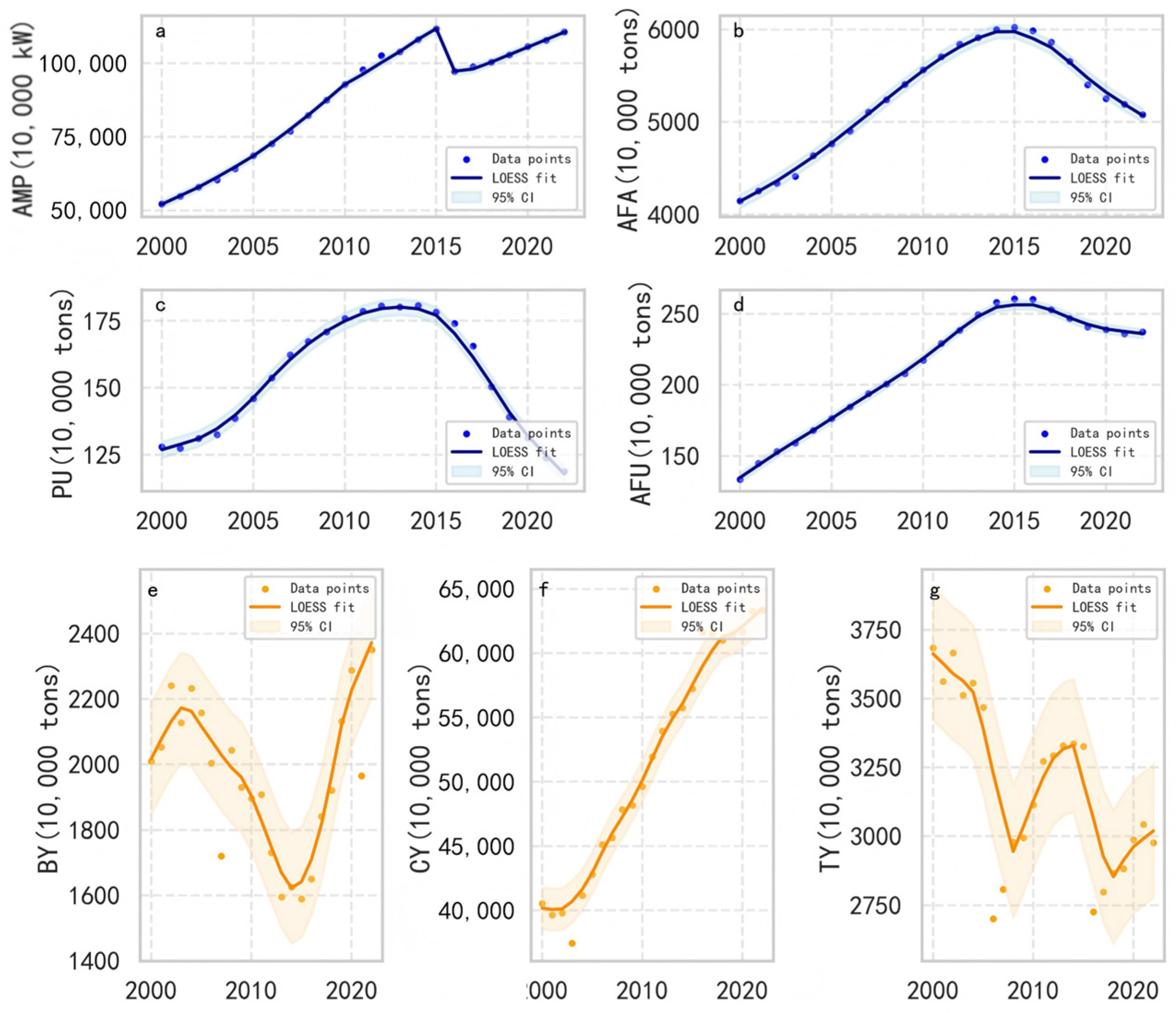
Over the past two decades, China’s agricultural material consumption has exhibited distinct phased characteristics and structural transformations (Figure 2a–d). Broadly speaking, these developments can be delineated into two primary phases: (1) High-input growth (2000–2015), focused on maximizing yield through increased agricultural inputs. (2) Green transformation and high-quality development (2016–present), marked by policies promoting ecological sustainability, leading to structural shifts in material use. Mechanization steadily advanced, while chemical inputs like fertilizers and pesticides peaked and then declined annually. This transition indicates that China’s agriculture is shifting from an extensive growth model that relies heavily on high-intensity agricultural inputs to a more refined model that emphasizes efficiency, environmental protection, and sustainability.

Over two decades, China’s food production has grown significantly, but its internal structure has diverged. Notably, yield trends of the three main crops showed distinct differentiation: (1) The trend of soybean yield is the most tortuous, exhibiting a distinct “V-shaped” pattern. Starting from its peak in 2002 at 22.413 million tons, soybean yield experienced a prolonged decline, reaching its lowest point around 2014 at approximately 16 million tons. Subsequently, the trend fundamentally reversed, with yields beginning a robust recovery, reaching 23.507 million tons in 2022—setting a new high in this cycle. (2) Cereal yield is fundamental to China’s food security. Between 2000 and 2022, cereal production increased from 405 million tons to 633 million tons, representing a growth of over 56%. Throughout this period, particularly after 2003, cereal yields entered a sustained growth phase spanning more than a decade, maintaining steady increases at a high level in recent years. (3) Unlike cereals and soybeans, tuber yield demonstrated an overall downward trend throughout the period. The yield fluctuated and declined from approximately 36.85 million tons in 2000 to around 29.78 million tons in 2022, representing an approximate decrease of 19%.

3.1.2. Spatial Pattern Analysis

This study examines four key categories of agricultural inputs in China from 2000 to 2022: the total power of agricultural machinery (AMP), the application amount of agricultural chemical fertilizers (AFA), pesticide usage (PU), and agricultural plastic film consumption (AFU). The analysis aims to characterize their spatial distribution and temporal variation.

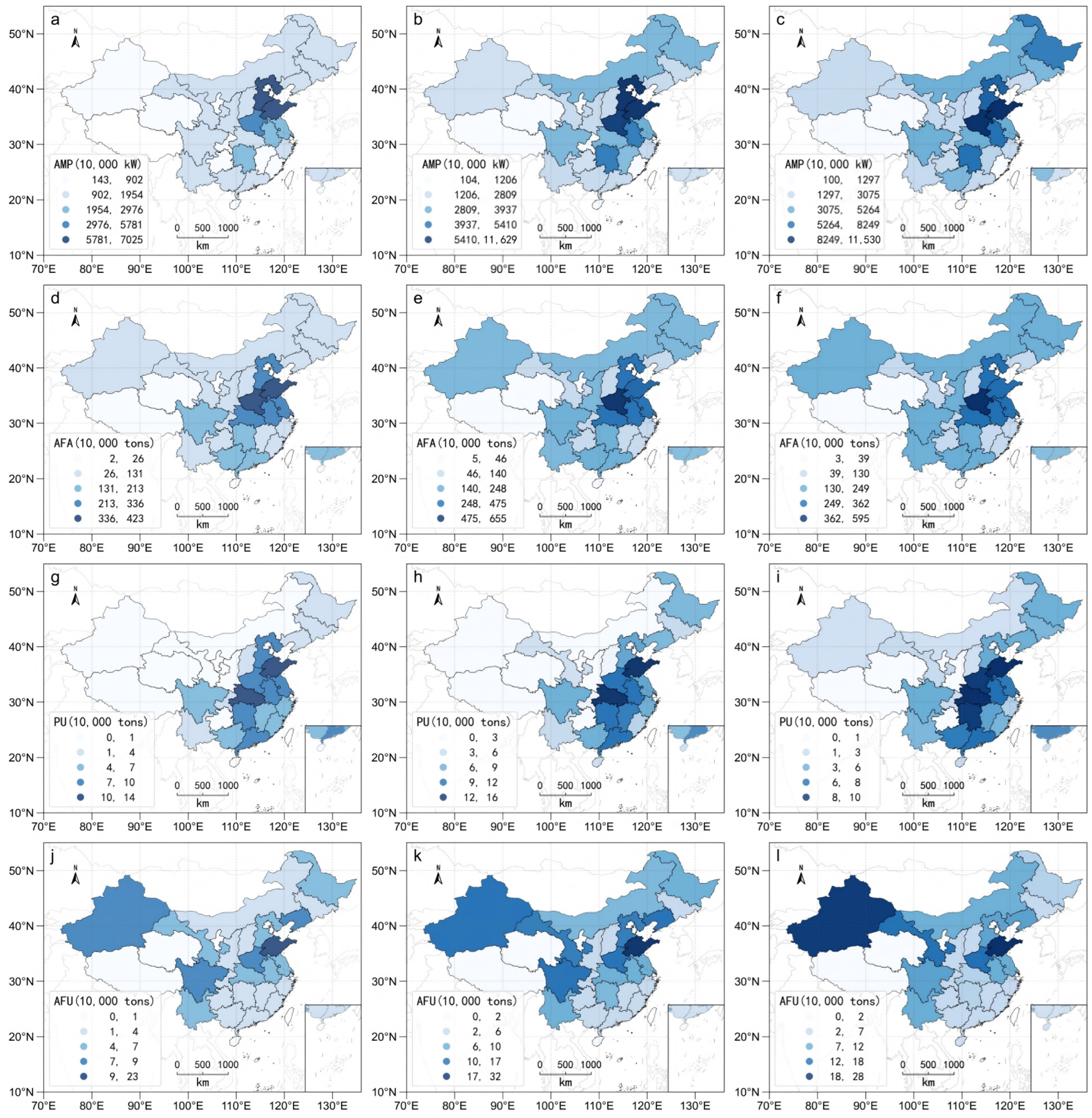
Total power of agricultural machinery serves as a key indicator of the intensity of agricultural mechanization. From 2000 (Figure 3a) to 2022 (Figure 3c), AMP showed a continuous growth trend with agglomeration in northern China: In 2000, high-value areas (≥57.81 × 10⁴ kW) were scattered in the Huang-Huai-Hai Plain and parts of Northeast China; in 2010 (Figure 3b), the high-power threshold evolved to ≥54.10 × 10⁴ kW, and the agglomeration degree in Northeast China and the Huang-Huai-Hai Plain increased significantly; in 2022, the AMP in core northern regions such as Heilongjiang and Shandong exceeded 82.49 × 10⁴ kW. In contrast, southern China has maintained a relatively low level of agricultural machinery power, likely due to the limitations imposed by fragmented terrain, which hinder the large-scale deployment of machinery.

Chemical fertilizer application has traditionally been vital for boosting food production but poses sustainability challenges. Temporally, its use first increased and then declined, reflecting China’s shift from yield maximization toward a green agriculture approach: In 2000 (Figure 3d), high-fertilizer application areas (≥3.36 × 10⁴ tons) were concentrated in the Huang-Huai-Hai Plain and the Sichuan Basin; in 2010 (Figure 3e), the scope of high-value areas further expanded (≥4.75 × 10⁴ tons), and the input intensity in major grain-producing areas continued to increase; in 2022 (Figure 3f), the AFA in core areas such as Shandong and Henan showed a moderate decline. Despite the observed decline, spatial path dependence remains evident. High multiple cropping areas show ongoing demand for soil nutrients, mainly from wheat and corn.

Pesticide usage reflects both the intensity of pest pressure and the evolution of pest management strategies. Spatially, PU consistently remained concentrated within the eastern agricultural ecological zones across all examined periods: In 2000 (Figure 3g), high PU areas (≥0.10 × 10⁴ tons) were only scattered in Shandong and Hubei; in 2010 (Figure 3h), the high-value threshold rose to ≥0.16 × 10⁴ tons, and the distribution in regions such as the Huang-Huai-Hai Plain and the Yangtze River Delta was more extensive (these regions have a high multiple cropping index and rich biodiversity of pests and diseases); in 2022 (Figure 3i), the PU in peak areas showed a moderate decline, which was consistent with the promotion of biological control and integrated pest management technologies. Due to the vulnerability of regional agricultural ecosystems to pests, spatial clustering persists.

Agricultural plastic films facilitate crop growth by enhancing water retention, regulating temperature, and performing other essential functions. Their application is especially critical in arid and cold regions characterized by harsh environmental conditions. In terms of time, AFU showed a significant expansion trend with agglomeration in arid northern areas: In 2000 (Figure 3j), high AFU areas (≥0.0023 × 10⁴ tons) were limited to Xinjiang and parts of North China; in 2010 (Figure 3k), the AFU in Xinjiang surged (≥0.0032 × 10⁴ tons), which may be related to the large-scale expansion of cash crops; in 2022 (Figure 3l), Xinjiang became the core area of agricultural plastic film usage in the country (≥0.0028 × 10⁴ tons), and the cultivation of corn and vegetables in the North China Plain also promoted the growth of agricultural plastic film usage. This pattern highlights the adaptability of film technology to environments with limited water and suboptimal temperatures, aligning with the regional expansion of cash crop cultivation.

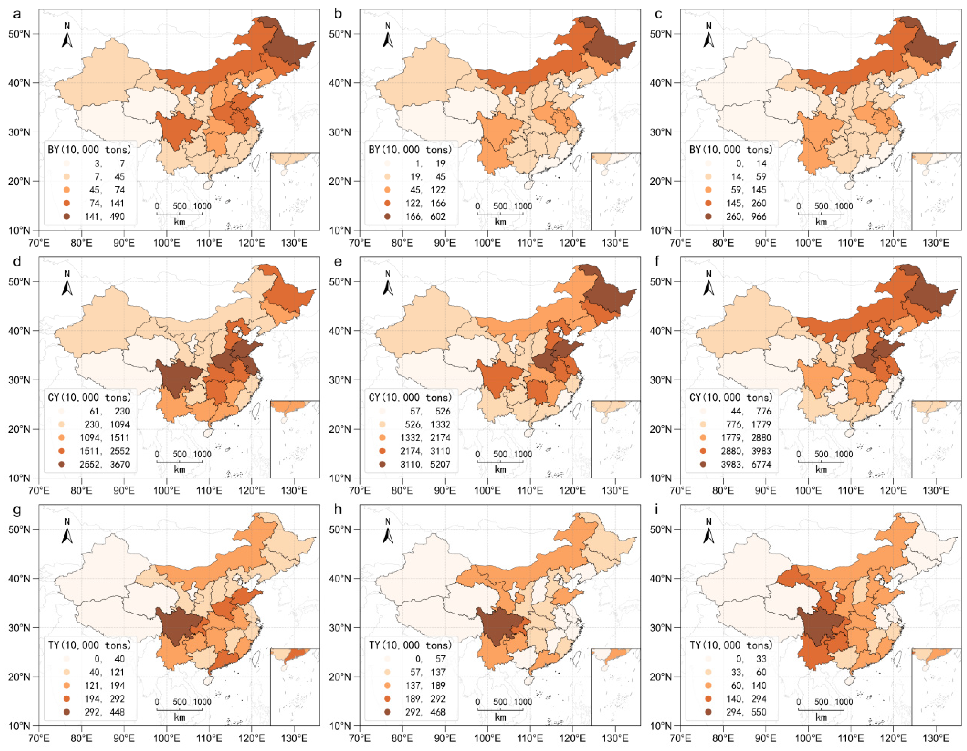
Soybean, a strategic legume crop, displays a spatiotemporal pattern of clustering in Northeast China, characterized by a gradual increase over time. Overall, soybean yields steadily grew. In 2000 (Figure 4a), high-value areas (≥1.41 million tons) were only concentrated in parts of Northeast China; In 2010 (Figure 4b), the high-value range increased (≥1.66 million tons), and the high-value range of the Northeast production area expanded slightly; In 2022 (Figure 4c), the high-value range further expanded (≥2.60 million tons), and the production capacity of the core production area increased significantly. The Northeast Plain has maintained high-value soybean areas due to its fertile soil and temperate climate, which are favorable for cultivation. Conversely, yields in most southern and northwestern regions remain relatively low.

Cereals constitute the core component of China’s grain production system, and their spatiotemporal yield patterns accurately reflect the fundamental principles governing major grain production. The growth rate was the most significant from 2000 to 2022. In 2000 (Figure 4d), high-value areas (≥25.52 million tons) were concentrated in the Huang-Huai-Hai Plain and the Northeast Plain; in 2010 (Figure 4e), the high-value range jumped to ≥31.10 million tons, and the high-value range of the main production areas expanded to the surrounding areas; in 2022 (Figure 4f), the high-value range exceeded ≥39.83 million tons, and the yield of the main production areas increased in a stepped manner. The high-value areas have been stably located in traditional main production areas such as the Huang-Huai-Hai Plain and the Northeast Plain for a long time. These regions benefit from ample arable land, favorable irrigation, and high-yield technologies supported by policies, forming large-scale cereal core areas. In contrast, southern rice regions, though high-yielding, have diverse planting structures, leading to different patterns of high-value agglomeration compared to northern dry-farming cereal areas.

Although total tuber output declined over the study period, the spatial concentration of high-yield areas in Southwest China became more evident. In 2000 (Figure 4g), high-value areas (≥2.92 million tons) were concentrated in Southwest China; in 2010 (Figure 4h), the high-value range increased slightly; in 2022 (Figure 4i), the high-value range further expanded (with an upper limit of 5.50 million tons), and the advantages of the Southwest main production area were continuously strengthened. The high-value areas have been centered on Southwest China for a long time. This region features numerous mountains and hills coupled with a humid climate, creating favorable conditions for the cultivation of tubers, which are characterized by their resistance to barren soils and strong adaptive capacity. While some North China regions saw tuber yield increases, primary production remains concentrated in Southwest China, emphasizing terrain and climate’s role in cultivation.

3.2. Nonlinear Impact Analysis

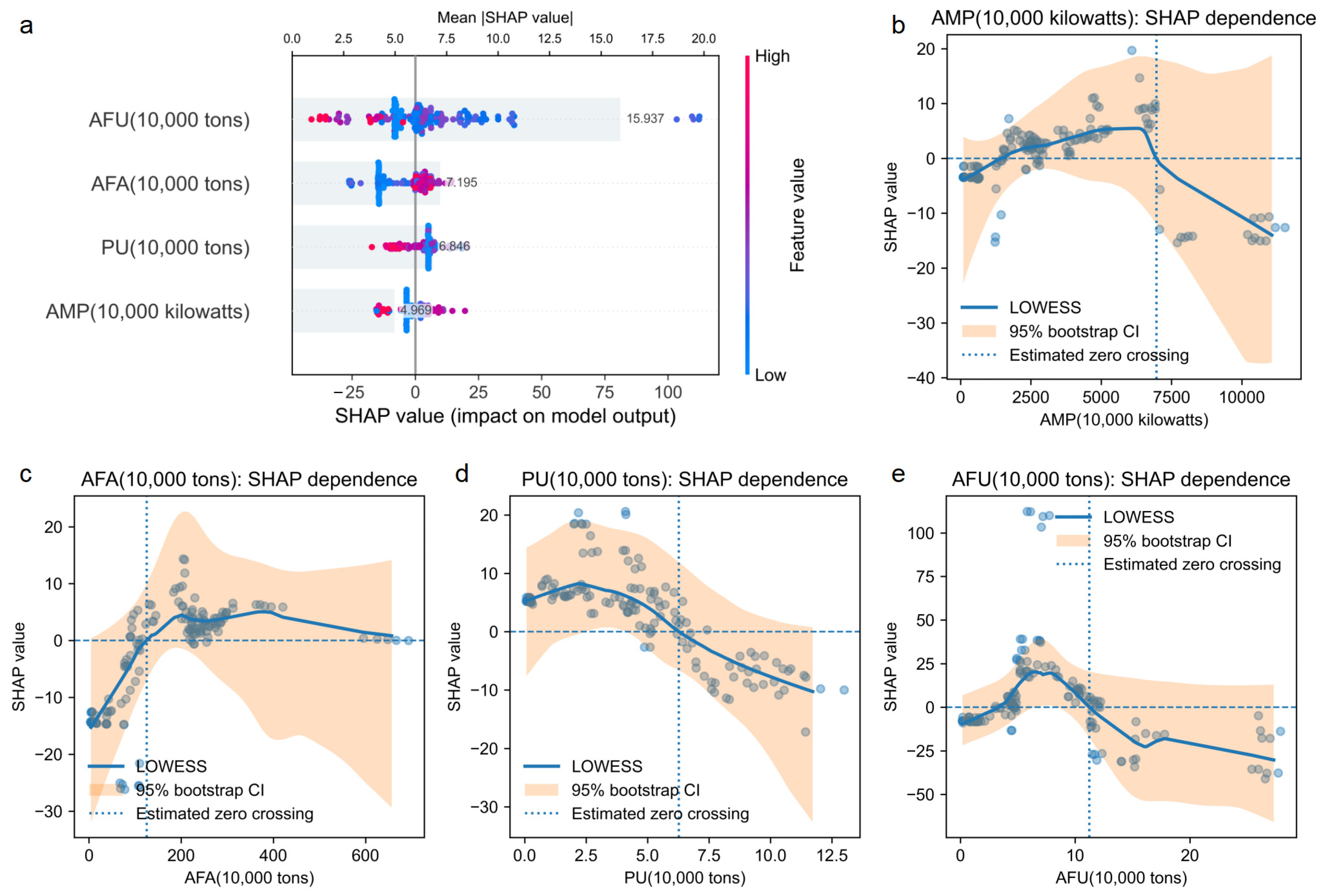
The model interpretability analysis indicates that AFU makes the highest average absolute SHAP contribution (15.937) to soybean yield predictions, followed by AFA (7.195), PU (6.846) and AMP (4.969) (Figure 5a). It should be noted that SHAP importance reflects the relative contribution of each variable to the model’s predictive output and does not directly indicate a causal effect. Figure 5b–e further reveal the nonlinear relationship between various agricultural inputs and their contribution to soybean yield predictions.

(1) Total power of agricultural machinery (Figure 5b): The LOWESS curve generally follows an inverted U-shaped pattern. At low to medium levels of mechanization, the SHAP contribution of total agricultural machinery power increases as inputs rise, reaching a high level in the medium-input range; thereafter, it gradually declines, turning negative at approximately 69.64 million kW. The 95% bootstrap confidence interval for this inflection point is 10.17 million to 80.74 million kW, with a bootstrap stability coefficient of 1.000. These results suggest that the contribution of mechanization inputs to soybean yield may be subject to diminishing returns; consequently, excessively high levels of total regional mechanical power do not necessarily translate into higher soybean yields.

(2) Agricultural chemical fertilizer application amount (Figure 5c): The relationship between fertilizer application and soybean yield forecasts exhibit a nonlinear pattern, shifting from a negative to a positive contribution, followed by a gradual decline in the marginal contribution. At lower fertilizer application rates, the SHAP value is generally negative; as fertilizer application increases, the LOWESS curve rises gradually and crosses the zero line at approximately 1.25 million tons. The 95% confidence interval for this inflection point is 0.69–2.89 million tons, with a Bootstrap stability coefficient of 1.000. Once this inflection point is exceeded, the SHAP contribution of fertilizer generally becomes positive, reaching a relatively high value at moderate input levels; in the higher input range, the curve gradually flattens or declines slightly, indicating a diminishing marginal contribution.

(3) Pesticide usage (Figure 5d): The relationship between pesticide application rates and soybean yield forecasts generally follows an inverted U-shaped pattern. At low to medium application rates, the SHAP contribution of pesticides is predominantly positive, peaking in the lower input range; as application rates increase further, this contribution gradually declines, turning negative at approximately 62.7 thousand tons. The 95% confidence interval for this inflection point is 5.7–96.9 thousand tons, with a Bootstrap stability coefficient of 0.970. Beyond this interval, the LOWESS curve generally remains negative and continues to decline, indicating that higher pesticide inputs are associated with lower predicted soybean yields.

(4) Agricultural plastic film usage (Figure 5e): There is a fairly clear ‘rise-then-fall’ relationship between the use of agricultural plastic film and the contribution to soybean yield forecasts. At extremely low levels of mulch film application, the SHAP contribution is close to zero or slightly negative; as usage increases, the contribution rises rapidly, peaking in the medium-input range. Thereafter, the curve declines markedly, turning from positive to negative at approximately 112.4 thousand tons. The 95% confidence interval for this inflection point is 20.1–125.9 thousand tons, with a Bootstrap stability coefficient of 0.995. Beyond this inflection point, the SHAP contribution of plastic mulch use is generally negative and declines further in the high-value range. This change may be related to the diminishing marginal returns of plastic mulch use and the constraints on soil structure, water movement and root growth caused by the accumulation of residual mulch.

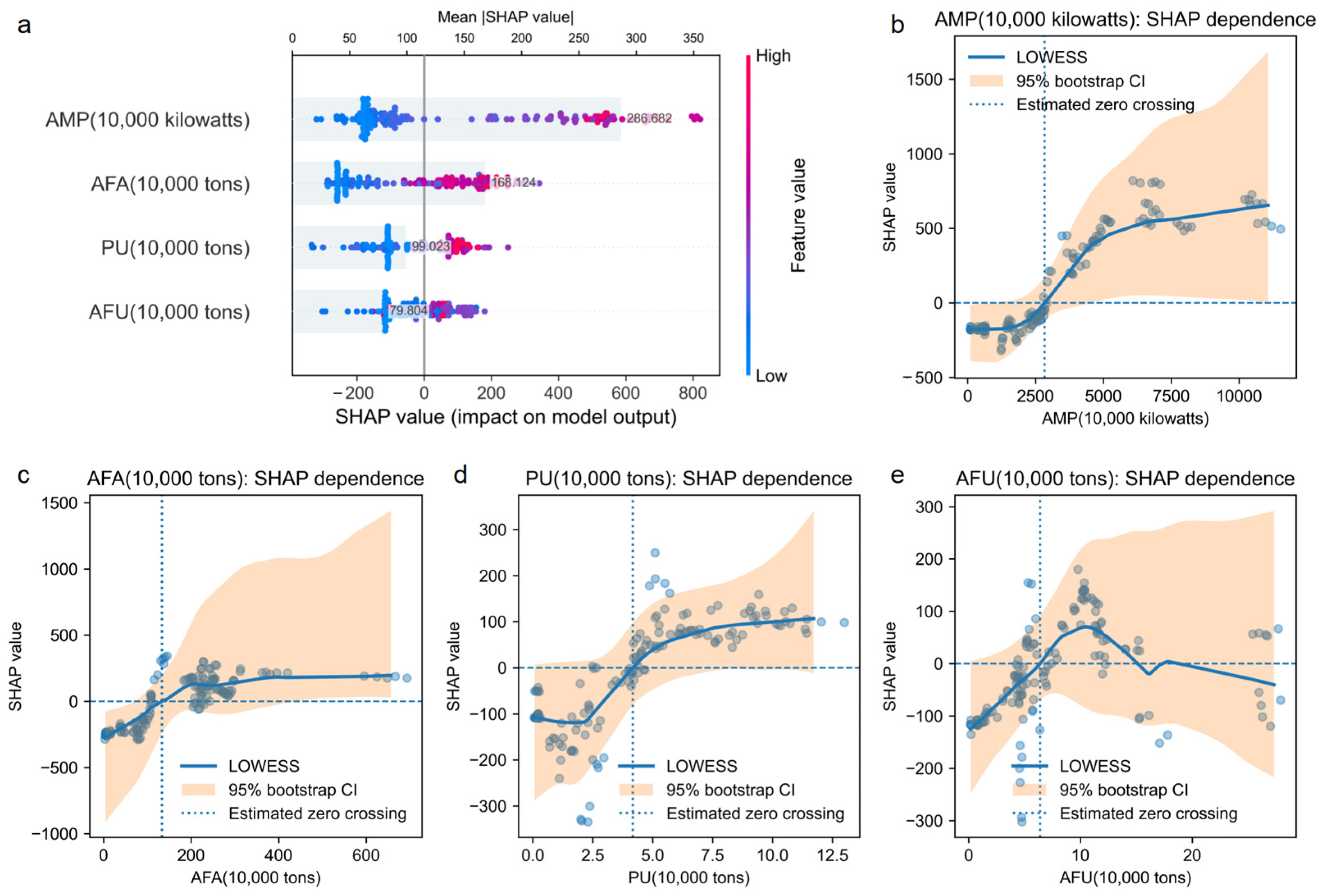
The model interpretability analysis indicates that AMP makes the highest average absolute SHAP (286.682) contribution to cereal yield predictions, followed by AFA (168.124), PU (99.023), and AFU (79.804) (Figure 6a). Figure 6b–e further illustrate the nonlinear relationship between the four categories of agricultural inputs and their predicted contributions to cereal yields.

(1) Total power of agricultural machinery (Figure 6b): At lower levels of mechanization, the SHAP values are generally negative, indicating that low levels of mechanization are associated with relatively low projected cereal yields. As total mechanical power increases, the LOWESS curve rises rapidly and crosses the zero line at approximately 28.34 million kW. The 95% bootstrap confidence interval for this inflection point is 14.05–45.80 million kW, with a bootstrap stability rate of 1.000, indicating that the zero-crossing was identified in all resampling runs. Thereafter, the SHAP contribution of total mechanical power continued to increase, gradually leveling off in the higher input range, while remaining positive overall. This may reflect the positive impact of mechanization on large-scale farming, operational efficiency, and the timeliness of production, although the marginal contribution diminishes during the high-input phase.

(2) Agricultural chemical fertilizer application amount (Figure 6c): The relationship between fertilizer application rates and cereal yield forecasts is nonlinear, characterized by a shift from a negative to a positive contribution, followed by a gradual decline in the marginal contribution. At lower fertilizer application rates, the SHAP value is generally negative; as fertilizer application rates increase, the LOWESS curve rises steadily and crosses the zero line at approximately 1.33 million tons. The 95% confidence interval for this inflection point is 0.82–3.10 million tons, with a Bootstrap stability coefficient of 0.985. Once this inflection point is exceeded, the SHAP contribution of fertilizer generally becomes positive, but the slope of the curve gradually decreases, indicating that its predictive contribution exhibits diminishing returns or is approaching saturation.

(3) Pesticide usage (Figure 6d): The relationship between pesticide usage and cereal yield forecasts generally shifts from negative to positive and gradually levels off. In the low-usage range, SHAP values are predominantly negative; as pesticide usage increases, the LOWESS curve rises markedly and turns positive at approximately 41.7 thousand tons. The 95% confidence interval for this inflection point is 17.9–78.5 thousand tons, with a Bootstrap stability coefficient of 0.980. Once this inflection point is exceeded, the SHAP contribution of the pesticide remains positive overall and gradually stabilizes at higher application levels.

(4) Agricultural plastic film usage (Figure 6e): There is a clear ‘rise-then-fall’ relationship between the use of agricultural plastic film and the predicted contribution to cereal yield. At lower input levels, the SHAP value is generally negative; as the use of agricultural film increases, the LOWESS curve rises rapidly and turns positive at approximately 63.9 thousand tons. The 95% confidence interval for this inflection point is 28.9–169.5 thousand tons, with a Bootstrap stability coefficient of 0.980. Thereafter, the SHAP contribution of agricultural film reaches a relatively high level at around 100,000 tons, before gradually declining; in the higher input range, it approaches zero or turns negative. These results suggest that moderate investment in agricultural film may be associated with higher projected cereal yields, but that its positive contribution may diminish at higher levels of investment.

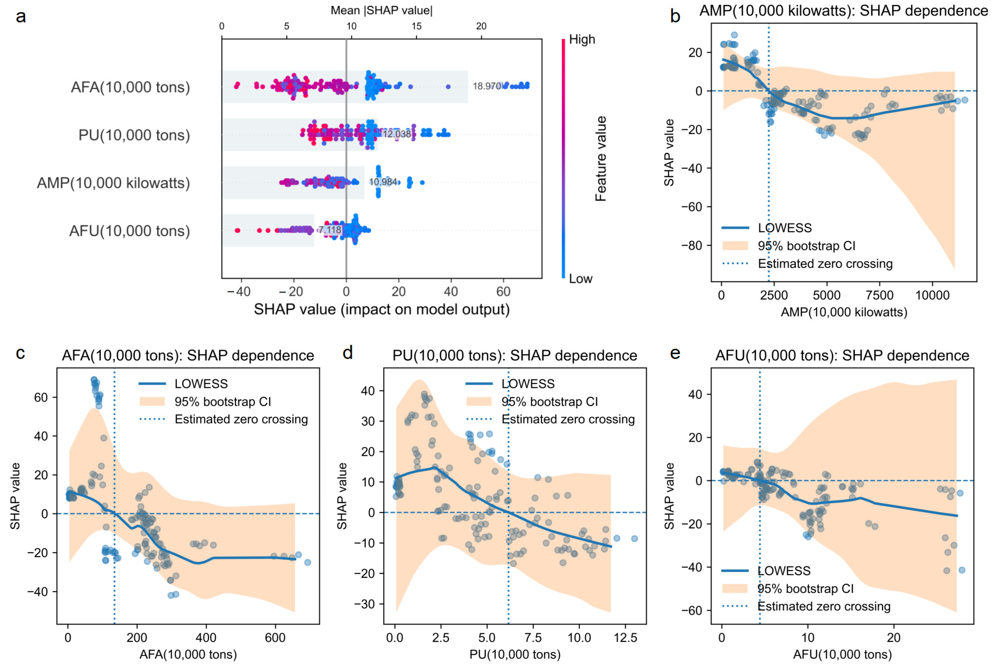
The model interpretability analysis indicates that AFA makes the highest average absolute SHAP (18.970) contribution to tuber crop yield predictions, followed by PU (12.038), AMP (10.984) and AFU (7.118) (Figure 7a). Figure 7b–e further illustrate the nonlinear relationship between various types of inputs and their predicted contribution to tuber crop yields.

(1) Total power of agricultural machinery (Figure 7b): At lower levels of mechanization, the LOWESS curve lies predominantly above the zero line; as total mechanical power increases, its SHAP contribution gradually declines, turning negative at approximately 22.46 million kW. The 95% bootstrap confidence interval for this inflection point is 7.11–57.61 million kW, with a bootstrap stability coefficient of 0.990. Once this inflection point is exceeded, the SHAP contribution of total mechanical power remains negative overall. This result suggests that once total mechanical power reaches a certain level, its marginal contribution to the prediction of tuber crop yields may diminish.

(2) Agricultural chemical fertilizer application amount (Figure 7c): At lower fertilizer application rates, the SHAP contribution of chemical fertilizers is generally positive, reaching relatively high levels in the low-input range; as fertilizer application rates increase further, the LOWESS curve continues to decline, turning negative at approximately 1.35 million tons. The 95% bootstrap confidence interval for this inflection point is 0.24–3.29 million tons, with a bootstrap stability coefficient of 0.990. Once this inflection point is exceeded, the SHAP contribution of fertilizer remains negative overall and gradually stabilizes at higher input levels.

(3) Pesticide usage (Figure 7d): At lower application rates, the SHAP contribution of pesticides is predominantly positive, peaking in the low-input range; as pesticide use increases, the LOWESS curve gradually declines, turning from positive to negative at approximately 61.6 thousand tons. The 95% bootstrap confidence interval for this inflection point is 7.88–83.00 thousand tons, with a bootstrap stability coefficient of 0.975. Once this inflection point is exceeded, the overall SHAP contribution of the pesticide remains negative and continues to decline as usage increases.

(4) Agricultural plastic film usage (Figure 7e): At very low input levels, its SHAP contribution is close to zero or slightly positive; as the use of agricultural film increases, the LOWESS curve gradually declines and turns negative at around 44.3 thousand tons. The 95% bootstrap confidence interval for this inflection point is 19.7–156.5 thousand tons, with a bootstrap stability coefficient of 0.975. Once this inflection point is exceeded, the SHAP contribution of agricultural film remains negative overall, and declines further in the high-input range.

Taken together, the feature-importance rankings and SHAP dependence analyses provide complementary information. The mean absolute SHAP values indicate which agricultural inputs contribute most strongly to the model’s predictive output, whereas the SHAP dependence plots further reveal how the model-predicted contributions of these inputs change across different input ranges. Therefore, the ranking results provide a basis for identifying priority inputs for crop-specific regulation, while the threshold curves indicate whether these priority inputs should be increased, reduced, or maintained within an appropriate range. In this sense, the added feature-importance rankings extend the interpretation beyond nonlinear response patterns by clarifying the relative management priority of different agricultural inputs across crops.

4. Discussion

4.1. Agricultural Inputs and Crop Production in China Exhibit Significant Spatiotemporal Heterogeneity

This study examines the temporal inflection points and spatial pattern evolution of agricultural inputs and crop production through an integrated spatiotemporal analytical framework. It not only corroborates the strategic shift in China’s macro-agricultural policies but also reveals the complex and multifaceted spatial-geographical characteristics underlying China’s green agricultural transformation and development. From the perspective of agricultural inputs, the application of chemical fertilizers, pesticides, and plastic mulch peaked around 2015 before commencing a decline, coinciding with the nationwide ‘Zero Growth Initiative’ vigorously promoted by the government [38]. Multiple studies indicate that this measure, implemented since 2015, has yielded significant results [28,39]. However, this process has not unfolded uniformly across regions. Compared to other areas, the Huang-Huai-Hai Plain and Yangtze River Delta regions, characterized by high cropping intensity, remain key yet challenging zones for reducing chemical fertilizer and pesticide use and mitigating their adverse effects. This is due to their sustained nutrient demands and complex ecological conditions. Against the backdrop of an overall decline in plastic mulch usage, regional increases have been observed in arid northwestern regions (Xinjiang) and cooler northern China. This trend stems from environmental characteristics and the expansion of economic crop cultivation in these areas, where mulch deployment addresses water scarcity and suboptimal temperature conditions. The rising total power of agricultural machinery, concentrated in northern China, highlights the development of large-scale grain production [40].

In terms of crop production, while overall crop output has increased, soybean yields have fluctuated, cereals have shown sustained growth, and tuber crops have experienced fluctuating declines. This pattern exhibits significant spatial variation [41,42]. The high-yield advantage zone for soybeans remains firmly established on the fertile Northeast Plain. The high-yield zones for cereals have long been stably distributed across traditional major production areas such as the Huang-Huai-Hai Plain and the Northeast Plain. Cereal production relies on ample arable land, well-developed irrigation systems and high-yield technologies supported by policy measures within these regions, thereby forming large-scale core grain production areas. Tuber crops, however, are primarily suited to humid hilly and mountainous areas in Southwest China.

By integrating the results of the spatial heterogeneity analysis with those of the SHAP threshold analysis, it can be observed that there is a significant coupling between spatial patterns and input threshold effects. Firstly, the Northeast Plain is not only a core high-yield region for cereal production, but also the area where the negative-to-positive threshold pattern of total agricultural machinery power in the cereal model is most likely to be triggered—the region has established a large-scale mechanized production system, with total machinery power having largely exceeded the critical threshold, and is currently in the ‘ascending phase’ where economies of scale from machinery investment are being realized. This coupling of spatial and threshold characteristics indicates that the Northeast Plain possesses the spatial conditions to further unlock its potential for increased cereal production through the continuous improvement of mechanization levels. Secondly, the arid regions of northwestern China (particularly Xinjiang) are areas where the use of agricultural plastic film is highly concentrated; consumption there far exceeds the national average and is likely to have entered, or be approaching, the ‘downward phase’ of the inverted U-shaped curve identified by the SHAP analysis. This coupling between spatial distribution and threshold values serves as a reminder to policymakers that there is an urgent practical need to promote the use of biodegradable mulch films and optimize mulching techniques in such regions, in order to avoid diminishing returns resulting from overuse. Thirdly, the Huang-Huai-Hai Plain and the middle and lower reaches of the Yangtze River, as regions traditionally characterized by high inputs of fertilizers and pesticides, have seen a downward trend in total input levels in recent years; however, the sustained demand for nutrients resulting from high cropping intensity means that input levels remain relatively high. In light of the SHAP analysis results, these regions need to formulate differentiated reduction strategies based on crop-specific thresholds, thereby avoiding a ‘one-size-fits-all’ approach. The aforementioned analysis of heterogeneity in agricultural inputs and crop production reveals that China’s sustainable food development pathway constitutes a spatially differentiated trajectory shaped by the interplay of geographical environments, cropping systems, and policy interventions. This provides a crucial spatial cognitive foundation for transitioning from a one-size-fits-all macro-management approach towards targeted, zoned and categorized regulatory measures.

4.2. The XGBoost-SHAP Framework Provides an Effective Approach for Identifying Nonlinear Input-Response Patterns Across Crops

This study employs an XGBoost-SHAP integrated analytical approach to systematically investigate the nonlinear threshold effects of key agricultural inputs in China’s crop production process, providing valuable insights for optimizing production practices. From a methodological perspective, XGBoost, as a powerful non-parametric machine learning model, automatically learns hidden higher-order interactions and nonlinear patterns within data without requiring prior assumptions. The introduction of the SHAP framework enables a more detailed analysis of the specific range of input thresholds across different crops and production conditions. XGBoost offers greater flexibility in terms of functional form and is capable of identifying nonlinear relationships and variable interactions without the need to specify a particular production function in advance; however, its predictive performance depends on the crop type. Specifically, XGBoost demonstrates the clearest advantage in the cereal model, shows some advantages in the tuber crop model, but does not exhibit a consistent advantage over the quadratic model in the soybean model.

It should also be noted that the interpretability of SHAP results needs to be understood within the structure of the fitted model. The multicollinearity diagnostics indicate that the agricultural input variables do not suffer from severe multicollinearity, although some variables show moderate correlations. Such correlations may affect the allocation of SHAP values among related predictors. Therefore, the SHAP-based importance rankings in this study should be interpreted as relative predictive contributions rather than as strictly independent causal effects. Similarly, the nonlinear thresholds derived from SHAP dependence plots represent conditional turning points under the observed combinations of agricultural inputs and regional production conditions, rather than isolated agronomic optima. Although PCA can be used as a complementary exploratory tool to identify latent input structures, it would transform the original input variables into composite components and thereby weaken the direct interpretation of crop-specific input thresholds. Therefore, this study retains the original agricultural input variables in the main XGBoost-SHAP analysis while explicitly acknowledging the potential interpretive influence of moderate multicollinearity.

From the perspective of research scale, although existing studies have examined the threshold effects of agricultural inputs, most investigations have been limited in scope or focused on a single subject. This study, conducted at a national scale across multiple agricultural commodities, overcomes the limitations of narrow geographical and commodity scopes inherent in local case studies [28,43,44,45]. It provides robust scientific evidence for formulating precise agricultural management strategies tailored to specific commodities and regional contexts.

4.3. It Is Both Necessary and Valuable to Conduct Comparative Analyses of How Different Crops Respond to Varying Input Thresholds

Unlike many existing studies that focus on single crops in specific regions or analyze the overall impact of inputs on crop yields, this study centers on three staple crops, soybeans, cereals, and tuber crops, and emphasizes their differentiated threshold responses to various agricultural inputs. This crop-comparative perspective extends previous studies that focused on single crops or aggregate crop output. The threshold results show that excessive pesticide and plastic-film use may be associated with negative predicted contributions to soybean yield, while fertilizer application shows a negative-to-positive pattern followed by diminishing marginal contribution. For tuber crops, excessive fertilizer, pesticide, and plastic-film use generally shows negative SHAP contributions beyond their respective thresholds. Excessive inputs not only fail to increase yields but also lead to reduced output through soil degradation, environmental pollution and physiological disorders in crops. These effects lead to economic and ecological harm, supporting the promotion of green practices like soil testing with targeted fertilization, Integrated Pest Management (IPM), and biodegradable plastic films. Although agricultural machinery symbolizes modernization, its application is constrained by crop-specific variations.

The role of mechanized operations also varies across crops. In the soybean model, agricultural plastic-film use shows the highest predictive contribution, whereas AMP has the lowest mean absolute SHAP value among the four core inputs. In the cereal model, however, AMP is the dominant predictor, indicating that the contribution of mechanization should be interpreted in a crop-specific manner rather than through a uniform modernization logic. Over-mechanization in tuber production increases tuber damage and leads to soil compaction, thereby reducing yields. This underscores the necessity for technological advancements to align with crop biology and specific agronomic requirements. It is crucial to advocate for the measured application of technology rather than its extreme utilization. The aforementioned characteristics underscore the necessity of conducting assessments and comparisons of the nonlinear threshold responses to differentiated input applications across different crops. Future policy formulation must implement precise regionalized management tailored to crop type, geographical location, and production scale, fully considering factors such as production conditions, crop health, and yield losses [46], thereby developing adaptive production strategies. Such measures would help reconcile food security, resource efficiency, and environmental protection.

4.4. Policy Implications

Combining the above findings, a threshold-informed policy mix may help reduce unnecessary agricultural input costs while supporting food security objectives and promoting the green transformation of agriculture.

(1) Policy formulation must be based on the crop characteristics and regional heterogeneity thresholds revealed by the SHAP model, establishing a precise regulatory system characterized by zoning, classification, and tiered management. This study reveals that the same input factor exerts markedly different effects on the yields of various crops, with their model-identified threshold ranges also being distinctly different. In practical terms, the mean absolute SHAP rankings can be used to identify which inputs should receive priority attention for each crop, while the threshold results can further guide the direction and intensity of input regulation. Consequently, future agricultural resource management policies must be grounded in a deep understanding of crop physiological characteristics and regional resource endowments, thereby establishing a refined regulatory framework. Firstly, a crop-oriented threshold-informed input guidance should be implemented. National and provincial agricultural technical guidelines may take into account significant regional variations in terms of cultivation scale and resource endowments, and conduct assessments of SHAP quantitative thresholds tailored to local agricultural production conditions. Based on the quantitative thresholds established through such research and assessment, differentiated reference ranges subject to local agronomic validation for agricultural input use should be formulated for different crops in each region, and these should be updated on an ongoing basis. National and provincial agricultural technical standards should establish crop- and region-specific recommended upper limits for agricultural input use, grounded in empirically derived quantitative thresholds, and subject to periodic revision. Secondly, implement a technology promotion pathway tailored to regional suitability. In large-scale grain-producing areas such as the Northeast Plain, efforts should continue to strengthen the development of high-standard farmland and provide subsidies for the research and development of large-scale intelligent agricultural machinery, thereby unlocking economies of scale. In scattered cultivation areas for soybeans or tuber crops, such as the hilly regions of southern China, the focus should shift towards promoting appropriate technologies including simplified machinery, biological nitrogen fixation techniques, and ecological ridge cultivation. This approach avoids the blind pursuit of mechanization rates.

(2) Reform existing subsidy mechanisms by shifting from universal cost subsidies to targeted incentives based on scientifically determined thresholds and green performance metrics. To achieve the objectives of green transition and high-quality development following the ‘zero growth’ phase, subsidy policies require systematic restructuring. The core of this restructuring lies in translating the ‘optimal range’ revealed by the SHAP model into an operational incentive-constraint mechanism. A pilot scheme could be introduced linking ‘green ecological subsidies’ to ‘input quota subsidies. For instance, additional ecological compensation incentives could be granted to farmers or cooperatives voluntarily limiting their application of fertilizers and pesticides below the model-identified threshold ranges for specific crops and regions as recommended by research. Secondly, explore the design of a ‘regional differentiated subsidy system’. Provinces may establish tailored subsidy packages aligned with the production thresholds of their dominant crops (such as soybeans in Heilongjiang, wheat in Henan, and potatoes in Gansu), based on scientifically assessed reasonable thresholds for agricultural input expenditure. Funding should be directed precisely toward the inputs most in need of regulation and the green technologies most worthy of promotion, thereby enhancing the overall effectiveness and marginal returns of subsidy policies.

(3) In response to the significant adverse effects arising when key inputs (particularly plastic mulch and chemical fertilizers) exceed threshold levels, increased investment in scientific research is required to accelerate the development and adoption of environmentally friendly alternative products and technological systems. SHAP analysis reveals that excessive inputs such as plastic film and chemical fertilizers exert a direct negative effect on soybean and tuber crop yields, highlighting the inherent risks of relying on traditional materials and technological approaches. Therefore, policy should actively steer a green substitution revolution in agricultural inputs. For plastic film-dependent regions in Northwest and North China, the government should establish dedicated programmed to collaborate with research institutions and enterprises in tackling the cost and technical barriers of fully biodegradable plastic film. This will accelerate the replacement of conventional plastic film, thereby addressing soil degradation and threshold negative effects caused by residual pollution at their root. Secondly, there should be a strong push to develop green inputs that maximize nutrient efficiency. To address the issue of excessive fertilizer use, policies should encourage and subsidies the production and adoption of new slow-release and controlled-release fertilizers, stable fertilizers, organic-inorganic compound fertilizers, and crop-specific formulations tailored to individual crop requirements. This will advance the integration of modernization and sustainability in grain production.

5. Conclusions and Future Research

5.1. Conclusions

This study systematically examined the spatiotemporal evolution of agricultural material use and the yields of cereals, soybeans, and tubers in China from 2000 to 2022. Using an interpretable machine learning model, it reveals the nonlinear and threshold effects of four key agricultural materials on these crops. The main conclusions are:

(1)

China’s agricultural development during the study period featured two phases. Pre-2015, it followed a high-input, high-output growth model with concurrent increases in material input and crop yields. Post-2016, a green transformation and high-quality development phase began. Policy-driven, chemical fertilizer and pesticide use declined after an inflection point, while agricultural machinery power continued to rise. This shift marks a transition from a factor-driven to an efficiency-focused model, balancing quantity and quality. However, the yield trends of the three major crops show distinct patterns. Cereal yields steadily increased, soybean yields exhibited a V-shaped recovery, and tuber yields fluctuated downward.

(2)

Spatial agglomeration of both agricultural material inputs and crop production has intensified. Total agricultural machinery power is concentrated in northern China’s flat terrain, suiting large-scale operations. Chemical fertilizer and pesticide application centers are historically in eastern China’s intensive farming regions. Although overall input use has declined, reliance on high-input practices persists. Agricultural plastic films are mainly used in northern China’s arid and cold regions. Core cereal areas are stable in the Northeast Plain and the Huang-Huai-Hai Plain; soybeans are concentrated in Northeast China; and tuber cultivation is concentrated in Southwest China’s mountainous and hilly areas.

(3)

The relationship between agricultural material inputs and crop yields is nonlinear and crop-specific, with evident threshold effects. For cereals, total agricultural machinery power is the most important predictor, followed by fertilizer application, pesticide use, and plastic-film use; its SHAP contribution turns positive at approximately 28.34 million kW and then gradually levels off. For soybeans, agricultural plastic-film use ranks first, followed by fertilizer application, pesticide use, and machinery power; its contribution turns negative beyond approximately 112.4 thousand tons. For tuber crops, fertilizer application is the dominant predictor, followed by pesticide use, machinery power, and plastic-film use; its contribution turns negative beyond approximately 1.35 million tons. These results indicate that input regulation should be differentiated by crop type and threshold range, and that the thresholds identified in this study should be interpreted as model-based reference points requiring local agronomic calibration rather than as uniform national standards.

5.2. Limitations and Future Research

This study offers valuable insights but has limitations. First, the data are mainly from provincial statistical units, which may mask heterogeneity at finer scales like city, county, or field. Second, the model considers only four main agricultural inputs, neglecting factors such as irrigation, labor, seed quality, and climate change. Climate factors have a direct effect on yield and interact in complex ways with inputs such as agricultural film and fertilizers. In the absence of a controlled climate baseline, the estimated thresholds may partly reflect initial environmental pressures rather than purely the effects of inputs; these limitations may restrict the comprehensiveness and interpretability. Although a sample size of 713 observations is considered moderate for machine learning tasks, we acknowledge the potential risk of overfitting when using complex models such as XGBoost with a dataset of this size. We have taken a number of measures to mitigate this risk; however, the aggregation at provincial level may still limit the level of detail in the research findings.

Future research can be improved in three directions. First, higher-resolution remote sensing and county-level data should be employed for detailed spatiotemporal analysis to better capture regional variations in agricultural activities. Second, multi-dimensional drivers, including high-resolution climate grids, socio-economic factors, and technological progress, could be integrated into a more comprehensive analytical framework. Causal identification methods such as double/debiased machine learning could then be applied to examine how climate-input interactions modulate the threshold effects identified in this study, thereby deepening the understanding of the complex dynamics of crop production. Third, more advanced regularization techniques could be adopted, and the predictive stability of this model benchmarked against that of other nonlinear models.

References

1. Campbell, B.M.; Beare, D.J.; Bennett, E.M.; Hall-Spencer, J.M.; Ingram, J.S.I.; Jaramillo, F.; Ortiz, R.; Ramankutty, N.; Sayer, J.A.; Shindell, D. Agriculture Production as a Major Driver of the Earth System Exceeding Planetary Boundaries. Ecol. Soc. 2017, 22, 8. [Google Scholar] [CrossRef]
2. Velazquez, J.A.; Negrutiu, I. Agriculture and Global Physicochemical Deregulation: Planetary Boundaries That Challenge Planetary Health. Lancet Planet. Health 2019, 3, E10–E11. [Google Scholar] [CrossRef] [PubMed]
3. Jin, S.; Ma, H.; Huang, J.; Hu, R.; Rozelle, S. Productivity, Efficiency and Technical Change: Measuring the Performance of China’s Transforming Agriculture. J. Product. Anal. 2010, 33, 191–207. [Google Scholar] [CrossRef]
4. Le, C.; Zha, Y.; Li, Y.; Sun, D.; Lu, H.; Yin, B. Eutrophication of Lake Waters in China: Cost, Causes, and Control. Environ. Manag. 2010, 45, 662–668. [Google Scholar] [CrossRef] [PubMed]
5. Zhan, X.; Shao, C.; He, R.; Shi, R. Evolution and Efficiency Assessment of Pesticide and Fertiliser Inputs to Cultivated Land in China. Int. J. Environ. Res. Public Health 2021, 18, 3771. [Google Scholar] [CrossRef] [PubMed]
6. Yin, G.; Liu, L.; Yuan, C. Assessing Environmental Risks for High Intensity Agriculture Using the Material Flow Analysis Method—A Case Study of the Dongting Lake Basin in South Central China. Environ. Monit. Assess. 2015, 187, 472. [Google Scholar] [CrossRef] [PubMed]
7. Zhang, X.; Davidson, E.A.; Mauzerall, D.L.; Searchinger, T.D.; Dumas, P.; Shen, Y. Managing Nitrogen for Sustainable Development. Nature 2015, 528, 51–59. [Google Scholar] [CrossRef] [PubMed]
8. Ma, L.; Zhang, Y.; Chen, S.; Yu, L.; Zhu, Y. Environmental Effects and Their Causes of Agricultural Production: Evidence from the Farming Regions of China. Ecol. Indic. 2022, 144, 109549. [Google Scholar] [CrossRef]
9. Sun, Y.; Huang, X.; Paerhati, B.; Zhou, K. Collaborative Solutions for Agricultural Water Pollution in Smallholder Economies: Farmers and Local Governments Unite. Agric. Water Manag. 2025, 313, 109499. [Google Scholar] [CrossRef]
10. Fuglie, K.O. Is Agricultural Productivity Slowing? Glob. Food Secur. 2018, 17, 73–83. [Google Scholar] [CrossRef]
11. Liu, Z.; Yang, D.; Wen, T. Agricultural Production Mode Transformation and Production Efficiency: A Labor Division and Cooperation Lens. China Agric. Econ. Rev. 2019, 11, 160–179. [Google Scholar] [CrossRef]
12. Tilman, D.; Cassman, K.G.; Matson, P.A.; Naylor, R.; Polasky, S. Agricultural Sustainability and Intensive Production Practices. Nature 2002, 418, 671–677. [Google Scholar] [CrossRef] [PubMed]
13. Mallinger, K.; Raubitzek, S.; Neubauer, T.; Lade, S. Potentials and Limitations of Complexity Research for Environmental Sciences and Modern Farming Applications. Curr. Opin. Environ. Sustain. 2024, 67, 101429. [Google Scholar] [CrossRef]
14. He, Q.; Sun, Y.; Yi, M.; Huang, H. How to Promote Agricultural Enterprises to Reduce the Use of Pesticides and Fertilizers? An Evolutionary Game Approach. Front. Sustain. Food Syst. 2023, 7, 1238683. [Google Scholar] [CrossRef]
15. Menegat, S.; Ledo, A.; Tirado, R. Greenhouse Gas Emissions from Global Production and Use of Nitrogen Synthetic Fertilisers in Agriculture. Sci. Rep. 2022, 12, 14490. [Google Scholar] [CrossRef] [PubMed]
16. Gong, J.; Du, H.; Sun, Y. Collaboration among Governments, Pesticide Operators, and Farmers in Regulating Pesticide Operations for Agricultural Product Safety. Agriculture 2023, 13, 2288. [Google Scholar] [CrossRef]
17. Daraban, G.M.; Hlihor, R.M.; Suteu, D. Pesticides vs. Biopesticides: From Pest Management to Toxicity and Impacts on the Environment and Human Health. Toxics 2023, 11, 983. [Google Scholar] [CrossRef] [PubMed]
18. Zhou, W.; Arcot, Y.; Medina, R.F.; Bernal, J.; Cisneros-Zevallos, L.; Akbulut, M.E.S. Integrated Pest Management: An Update on the Sustainability Approach to Crop Protection. ACS Omega 2024, 9, 41130–41147. [Google Scholar] [CrossRef] [PubMed]
19. Wang, Z.; Ye, T.; Wang, J.; Cheng, Z.; Shi, P. Contribution of Climatic and Technological Factors to Crop Yield: Empirical Evidence from Late Paddy Rice in Hunan Province, China. Stoch. Environ. Res. Risk Assess. 2016, 30, 2019–2030. [Google Scholar] [CrossRef]
20. Fan, F.; van der Werf, W.; Makowski, D.; Lamichhane, J.R.; Huang, W.; Li, C.; Zhang, C.; Cong, W.-F.; Zhang, F. Cover Crops Promote Primary Crop Yield in China: A Meta-Regression of Factors Affecting Yield Gain. Field Crop. Res. 2021, 271, 108237. [Google Scholar] [CrossRef]
21. Suh, D.H.; Moss, C.B. Examining the Input and Output Linkages in Agricultural Production Systems. Agriculture 2021, 11, 54. [Google Scholar] [CrossRef]
22. Liu, Z.; Di, L.; Yang, R.; Guo, L.; Zhang, C.; Li, H.; Shao, B. In-Season Crop Yield Prediction: State of the Art and Future Research Direction. Int. J. Appl. Earth Obs. Geoinf. 2026, 146, 105129. [Google Scholar] [CrossRef]
23. Jabed, M.A.; Murad, M.A.A. Crop Yield Prediction in Agriculture: A Comprehensive Review of Machine Learning and Deep Learning Approaches, with Insights for Future Research and Sustainability. Heliyon 2024, 10, e40836. [Google Scholar] [CrossRef] [PubMed]
24. Hernández Hernández, G.C.; Gómez Gómez, J.; Jiménez-Cabas, J. Predictive Models Based on Artificial Intelligence to Estimate Crop Yield: A Literature Review. Agriculture 2025, 15, 2438. [Google Scholar] [CrossRef]
25. Shawon, S.M.; Ema, F.B.; Mahi, A.K.; Niha, F.L.; Zubair, H. Crop Yield Prediction Using Machine Learning: An Extensive and Systematic Literature Review. Smart Agric. Technol. 2025, 10, 100718. [Google Scholar] [CrossRef]
26. Chen, T.; Guestrin, C. Xgboost: A Scalable Tree Boosting System. In Proceedings of the 22nd ACM Sigkdd International Conference on Knowledge Discovery and Data Mining; Association for Computing Machinery: New York, NY, USA, 2016; pp. 785–794. [Google Scholar] [CrossRef]
27. Deng, N.; Grassini, P.; Yang, H.; Huang, J.; Cassman, K.G.; Peng, S. Closing Yield Gaps for Rice Self-Sufficiency in China. Nat. Commun. 2019, 10, 1725. [Google Scholar] [CrossRef] [PubMed]
28. Cheng, Z.; Zhu, M.; Cai, J. Reducing Fertilizer and Pesticide Application through Mandatory Agri-Environmental Regulation: Insights from “Two Zero” Policy in China. Environ. Impact Assess. Rev. 2025, 110, 107716. [Google Scholar] [CrossRef]
29. Asgary, S.; Aghashariatmadari, Z. Sensitivity Analysis of Rainfed Wheat Yield to Climatic Indices Using the Interpretable XGBoost–SHAP Model under Climate Change Conditions: Zanjan Province Case Study. Iran. J. Soil Water Res. 2026, 57, 1–20. [Google Scholar] [CrossRef]
30. Barredo Arrieta, A.; Diaz-Rodriguez, N.; Del Ser, J.; Bennetot, A.; Tabik, S.; Barbado, A.; Garcia, S.; Gil-Lopez, S.; Molina, D.; Benjamins, R.; et al. Explainable Artificial Intelligence (XAI): Concepts, Taxonomies, Opportunities and Challenges toward Responsible AI. Inf. Fusion 2020, 58, 82–115. [Google Scholar] [CrossRef]
31. Wang, M.; Li, Y.; Yuan, H.; Zhou, S.; Wang, Y.; Ikram, R.M.A.; Li, J. An XGBoost-SHAP Approach to Quantifying Morphological Impact on Urban Flooding Susceptibility. Ecol. Indic. 2023, 156, 111137. [Google Scholar] [CrossRef]
32. Sun, Y.; Xie, L.; Huang, M.; Hu, R. Understanding Multi-Disaster Impacts on China’s Grain Production for Food Security: An XGBoost-SHAP Approach. Food Energy Secur. 2026, 15, e70237. [Google Scholar] [CrossRef]
33. Meng, M.; Yu, L.; Yu, X. Machinery Structure, Machinery Subsidies, and Agricultural Productivity: Evidence from China. Agric. Econ. 2024, 55, 223–246. [Google Scholar] [CrossRef]
34. Guo, Y.; Wang, J. Spatiotemporal Changes of Chemical Fertilizer Application and Its Environmental Risks in China from 2000 to 2019. Int. J. Environ. Res. Public Health 2021, 18, 11911. [Google Scholar] [CrossRef] [PubMed]
35. Zuo, X.; Li, H.; Wang, C.; Cao, A.; Wen, H. Path to Reducing Pesticide Input: Is Agricultural Production Outsourcing Effective? Ecol. Econ. 2026, 246, 109002. [Google Scholar] [CrossRef]
36. Huang, T.; Wu, Q.; Yuan, Y.; Zhang, X.; Sun, R.; Hao, R.; Yang, X.; Li, C.; Qin, X.; Song, F.; et al. Effects of Plastic Film Mulching on Yield, Water Use Efficiency, and Nitrogen Use Efficiency of Different Crops in China: A Meta-Analysis. Field Crop. Res. 2024, 312, 109407. [Google Scholar] [CrossRef]
37. Fan, J.; Liu, B.; Lei, T.; Sun, Y.; Ma, Y.; Guo, R.; Chen, D.; Zhou, K.; Li, S.; Gao, X. Exploring How Economic Level Drives Urban Flood Risk. Nat. Commun. 2025, 16, 4857. [Google Scholar] [CrossRef] [PubMed]
38. Jin, S.; Zhou, F. Zero Growth of Chemical Fertilizer and Pesticide Use: China’s Objectives, Progress and Challenges. J. Resour. Ecol. 2018, 9, 50–58. [Google Scholar] [CrossRef]
39. van Wesenbeeck, C.F.A.; Keyzer, M.A.; van Veen, W.C.M.; Qiu, H. Can China’s Overuse of Fertilizer Be Reduced without Threatening Food Security and Farm Incomes? Agric. Syst. 2021, 190, 103093. [Google Scholar] [CrossRef]
40. Wang, X.; Yamauchi, F.; Huang, J.; Rozelle, S. What Constrains Mechanization in Chinese Agriculture? Role of Farm Size and Fragmentation. China Econ. Rev. 2020, 62, 101221. [Google Scholar] [CrossRef]
41. Qi, Y.; Qiang, W.; Ma, X. Spatiotemporal Pattern Evolution of Food and Nutrient Production in China. Foods 2023, 12, 3791. [Google Scholar] [CrossRef] [PubMed]
42. Li, Y.; Yang, Y.; Liu, L.; Pan, W. New Spatial Pattern of Food Production and Its Climatic Disaster Risk in China. Trans. Chin. Soc. Agric. Eng. 2026, 42, 1–13. [Google Scholar] [CrossRef]
43. Yang, Z.; Hu, Y.; Zhang, S.; Raza, S.; Wei, X.; Zhao, X. The Thresholds and Management of Irrigation and Fertilization Earning Yields and Water Use Efficiency in Maize, Wheat, and Rice in China: A Meta-Analysis (1990–2020). Agronomy 2022, 12, 709. [Google Scholar] [CrossRef]
44. Tian, M.; Zheng, Y.; Sun, X.; Zheng, H. A Research on Promoting Chemical Fertiliser Reduction for Sustainable Agriculture Purposes: Evolutionary Game Analyses Involving “Government, Farmers, and Consumers”. Ecol. Indic. 2022, 144, 109433. [Google Scholar] [CrossRef]
45. Hu, Y.; Liu, Y. Impact of Fertilizer and Pesticide Reductions on Land Use in China Based on Crop-Land Integrated Model. Land Use Policy 2024, 141, 107155. [Google Scholar] [CrossRef]
46. Savary, S.; McRoberts, N.; Esker, P.D.; Willocquet, L.; Teng, P.S. Production Situations as Drivers of Crop Health: Evidence and Implications. Plant Pathol. 2017, 66, 867–876. [Google Scholar] [CrossRef]
Figure 1. Overall framework of this study.
Agriculture 16 01472 g001
Figure 2. Trends of agricultural material input and crop yield over time (2000–2022). (a) Total power of agricultural machinery; (b) agricultural chemical fertilizer application amount; (c) pesticide usage; (d) agricultural plastic film usage; (e) soybean yield; (f) cereal yield; (g) tuber yield.
Agriculture 16 01472 g002
Figure 3. Spatial patterns of agricultural material consumption in China. (a) Spatial pattern of total power of agricultural machinery in 2000; (b) spatial pattern of total power of agricultural machinery in 2010; (c) spatial pattern of total power of agricultural machinery in 2022; (d) spatial pattern of agricultural chemical fertilizer application amount in 2000; (e) spatial pattern of agricultural chemical fertilizer application amount in 2010; (f) spatial pattern of agricultural chemical fertilizer application amount in 2022; (g) spatial pattern of pesticide usage in 2000; (h) spatial pattern of pesticide usage in 2010; (i) spatial pattern of pesticide usage in 2022; (j) spatial pattern of agricultural plastic film usage in 2000; (k) spatial pattern of agricultural plastic film usage in 2010; (l) spatial pattern of agricultural plastic film usage in 2022.
Agriculture 16 01472 g003
Figure 4. Spatial patterns of crop yield in China. (a) Spatial pattern of soybean yield in 2000; (b) spatial pattern of soybean yield in 2010; (c) spatial pattern of soybean yield in 2022; (d) spatial pattern of cereal yield in 2000; (e) spatial pattern of cereal yield in 2010; (f) spatial pattern of cereal yield in 2022; (g) spatial pattern of tuber yield in 2000; (h) spatial pattern of tuber yield in 2010; (i) spatial pattern of tuber yield in 2022.
Agriculture 16 01472 g004
Figure 5. Impact of agricultural material consumption on soybean yield. (a) SHAP value bee swarm plot; (b) impact of total power of agricultural machinery on soybean yield; (c) impact of agricultural chemical fertilizer application amount on soybean yield; (d) impact of pesticide usage on soybean yield; (e) impact of agricultural plastic film usage on soybean yield.
Agriculture 16 01472 g005
Figure 6. Impact of agricultural material consumption on cereal yield. (a) SHAP value bee swarm plot; (b) impact of total power of agricultural machinery on cereal yield; (c) impact of agricultural chemical fertilizer application amount on cereal yield; (d) impact of pesticide usage on cereal yield; (e) impact of agricultural plastic film usage on cereal yield.
Agriculture 16 01472 g006
Figure 7. Impact of agricultural material consumption on tuber yield. (a) SHAP value bee swarm plot; (b) impact of total power of agricultural machinery on tuber yield; (c) impact of agricultural chemical fertilizer application amount on tuber yield; (d) impact of pesticide usage on tuber yield; (e) impact of agricultural plastic film usage on tuber yield.
Agriculture 16 01472 g007