A Time-Aware Machine Learning Framework for Behavioral Anomaly Monitoring and Short-Horizon Forecasting in Goats Using RFID-Derived Activity Data

Abstract

Precision livestock farming requires monitoring approaches that extend beyond static activity thresholds to enable dynamic, animal-level decision support. A time-aware machine learning framework was developed to transform RFID-derived goat activity records into an interpretable behavioral monitoring system. Time-stamped activity data were processed into temporal features such as lagged activity, rolling mean, activity change, and elapsed-time variables to capture short-term behavioral history. The framework integrated latent-state discovery, fuzzy-uncertainty analysis, transition modeling, supervised classification, short-horizon forecasting, and dashboard-based alert visualization within a predictive dashboard-based monitoring framework. Four latent behavioral clusters were identified, with the dominant cluster representing a stable low-activity baseline and accounting for 77.88% of observations. Boundary-zone analysis indicated that 7.30% of observations were in transitional regions, while fuzzy clustering classified 21.42% as uncertain or mixed-state points, suggesting gradual shifts in activity. Transition analysis revealed greater persistence in baseline states and lower persistence in high-activity/non-baseline states, which exhibited the highest volatility and entropy. Using nested time-blocked validation, Random Forest predicted future high-activity/non-baseline onset with AUC values of 0.869 and 0.841 for 5 and 10 min horizons, respectively. These results demonstrate that activity instability can be detected and forecasted over short horizons, supporting behavior-based monitoring. However, external biological validation is still required before implementation as a health- or disease-detection system.

1. Introduction

Goat production systems increasingly face combined pressure to improve productivity, animal welfare, health surveillance, and labor efficiency all at the same time. In that setting, precision livestock farming (PLF) has become attractive because it links sensing technologies, analytics, and decision support to animal-level management rather than relying only on periodic visual inspection. More recent PLF studies also makes it clear that these systems are moving beyond simple alarms triggered by abnormal states toward integrated decision support, where sensor data, algorithms, and interfaces are expected to work together in a practical monitoring pipeline [1,2,3].

Recent agricultural AI studies outside livestock also show a similar shift from simple detection toward more specialized, interpretable, and task-oriented decision-support systems. For example, PestScope, an exclusion-aware large multimodal model for fine-grained agricultural pest segmentation, illustrates how agricultural AI is increasingly being designed to combine perception, task-specific reasoning, and interpretable output generation for applied decision support [4]. Although PestScope addresses crop-pest segmentation rather than livestock behavior monitoring, it provides useful broader context for the present study because both lines of work reflect the movement from isolated classification toward more integrated AI-based agricultural monitoring frameworks.

For goats, this shift is especially important because continuous direct observation of every individual is completely impractical in both intensive and semi-intensive systems. Behavioral changes can be among the earliest visible signs of discomfort, stress, disturbance, illness, or altered welfare status, which makes automated behavioral surveillance highly relevant for real-time herd management and targeted intervention. Goat-focused studies have already shown that machine learning, computer vision, and sensor-based systems can classify behaviors, such as eating, drinking, active, inactive, and abnormal movement, with promising accuracy. Video-based deep learning frameworks have recognized group-housed goat behaviors in real time, and on-farm Internet of Things (IoT) machine learning systems have also been developed for welfare-oriented goat monitoring [5]. More recent work has extended this line further through accelerometer-based classification of goat activity and lightweight real-time recognition of multiple dairy goat behaviors, including abnormal ones [6,7,8,9]. Because prior goat-monitoring studies differ in sensor modality, behavioral labels, validation design, and outcome definition, direct numerical performance comparison is not fully appropriate. Therefore,

Table 1. Comparative summary of related goat behavior-monitoring frameworks and the present RFID-derived temporal forecasting framework.

Study	Sensor/Input	Main Task	Forecasting?	Validation Focus	Main Distinction from Present Study
Jiang et al. [5]	Video/computer vision	Recognized eating, drinking, active, and inactive behaviors in group-housed goats	No	Behavior recognition from video	Focused on current behavior recognition, not state transitions or future forecasting.
Hollevoet et al. [7]	Accelerometer sensors	Compared neural networks, CNN, and hybrid models for goat activity analysis	No	Activity classification using wearable sensors	Focused on accelerometer-based activity classification, not RFID-based transition modeling or short-horizon forecasting.
Chen et al. [10]	Computer vision/video	Online behavior recognition system for Liaoning Cashmere goats	No	Deep learning detection and online monitoring	Reported YOLOv8n average detection accuracy of 95.31% and improved model accuracy of 98.11%; focused on real-time visual behavior recognition.
Wang et al. [8]	Computer vision/video	Lightweight behavior recognition for dairy goats	No	Real-time visual behavior recognition	Focused on lightweight deep learning for recognizing dairy goat behaviors, including abnormal behaviors.
Mauny et al. [9]	Accelerometer data	Pipeline for detecting dairy goat behavior from accelerometer data	No	Preprocessing and behavior detection	Emphasized preprocessing choices and noted that small same-context datasets are not enough for strong generalizable models.
Méndez et al. [11]	Accelerometer data	Goat behavior prediction/classification using preprocessing and machine learning	Not the same as short-horizon state forecasting	Sensor feature and preprocessing-based prediction	Recent accelerometer-based goat behavior work; differs from the present RFID-based latent-state and transition framework.
Méndez et al. [12]	Computer vision/video	Multi-object detection for goat behavior identification	No	Object-detection models for eating, standing, drinking, and lying	Used 10,740 labeled annotations and compared transformer- and CNN-based object-detection models; not RFID-based forecasting.
Present study	RFID-derived activity stream	Latent-state modeling, transition analysis, and short-horizon activity-instability forecasting	Yes; 5 and 10 min horizons	Nested time-blocked forecasting, baseline comparison, feature importance	Integrated RFID-derived temporal features, latent states, uncertainty, transition dynamics, and short-horizon forecasting into one framework.

provides a structured comparison of related goat behavior-monitoring frameworks in terms of sensor type, modeling objective, temporal modeling, forecasting capability, and the main methodological distinction of the present study.

This comparison shows that previous goat-monitoring studies have mainly focused on recognition or classification of current behavior, whereas the present study integrates RFID-derived temporal features, latent-state discovery, uncertainty analysis, transition dynamics, and short-horizon forecasting within one monitoring workflow.

Recent goat-focused studies have further strengthened this direction using both wearable sensors and computer vision. Méndez et al. [11] developed a goat behavior prediction approach using accelerometer data, emphasizing the importance of preprocessing choices, sensor-based feature extraction, and machine learning model selection for reliable behavior classification. Similarly, Méndez et al. [12] evaluated multi-object detection models for automated goat behavior identification in intensive farming facilities, showing the growing role of computer vision and object-detection architectures for monitoring goat behavior from video data. Together, these recent accelerometer- and computer vision-based studies show that goat behavior monitoring is rapidly moving toward automated prediction systems; however, much of the current work still focuses mainly on classifying observed behavior rather than modeling behavioral state transitions, uncertainty, and short-horizon future activity instability.

Even so, most prior work in this space has focused mainly on recognition of predefined behaviors at isolated time points [13]. In other words, the dominant question has usually been: what behavior is the animal showing right now? This has been an important step, but it does not fully address a more operational question for precision management: is the animal behaviorally stable, drifting, escalating, recovering, or approaching a high-risk condition? Reviews of accelerometer-based livestock behavior prediction emphasize that animal behavior is best understood when raw activity streams are processed with explicit attention to time structure, preprocessing, and model design, rather than reduced to static summaries alone [14,15]. Likewise, broader reviews of deep learning for livestock behavior recognition show that the field has grown rapidly, but much of the literature still centers on classification performance rather than dynamic state inference and deployment-oriented interpretation [16].

This gap matters because abnormal or unstable behavior is rarely a purely static event. In biological systems, disturbance often develops progressively, passes through intermediate conditions, and then either intensifies or returns toward baseline. For that reason, a framework that only labels individual moments may miss the temporal structure that is most useful for early warning. In small ruminants, where welfare challenges can involve disease, nutritional stress, maternal problems, environmental impacts, and agonistic interactions, PLF approaches are increasingly being discussed as tools for earlier and more objective detection of meaningful change [17]. From an AI standpoint, this shifts the task from simple behavior classification toward time-aware behavioral intelligence, where the goal is to infer state, quantify uncertainty, model transitions, and anticipate high-activity/non-baseline state emergence from recent behavioral history.

A second limitation in the current goat-monitoring literature is that activity-monitoring systems are often described as intelligent or digital decision-support tools, but many remain focused on passive data display or single-time-point behavior classification. In livestock systems, digital twins have been proposed as continuously updated virtual representations that can support simulation, prediction, and management decisions rather than passive monitoring alone [1,18]. Related work in dairy cattle has also shown how sensor data and behavioral modeling can contribute to digital twin development across the animal lifecycle [19]. However, the present study does not claim to present a fully operational or closed-loop digital twin, because it does not include real-time sensor streaming, simulation of alternative management actions, automated intervention, or bi-directional feedback from clinical, physiological, or environmental sensors. Instead, the present work is framed as a time-aware machine learning and predictive dashboard framework for goat behavioral monitoring.

Therefore, the objective of this study was to develop a time-aware machine learning framework for goat behavioral monitoring and short-horizon activity-instability forecasting using RFID-derived activity data. The framework treated goat activity as a dynamic behavioral process rather than a single-time-point classification task. Specifically, the study aimed to identify latent activity states from RFID-derived behavioral streams, quantify uncertainty and persistence, characterize transition dynamics, evaluate whether recent temporal history could forecast future high-activity/non-baseline state onset, and translate these outputs into an interpretable prototype dashboard for animal-level decision support. Because the dataset represents a behavior-first monitoring context, the framework is intended primarily for activity-instability detection and decision support rather than direct clinical diagnosis. The core analytical models are standard machine learning methods, including clustering and supervised forecasting algorithms, but they are integrated into a broader time-aware behavioral monitoring workflow [1,2].

2. Materials and Methods

2.1. Study Design and Analytical Framework

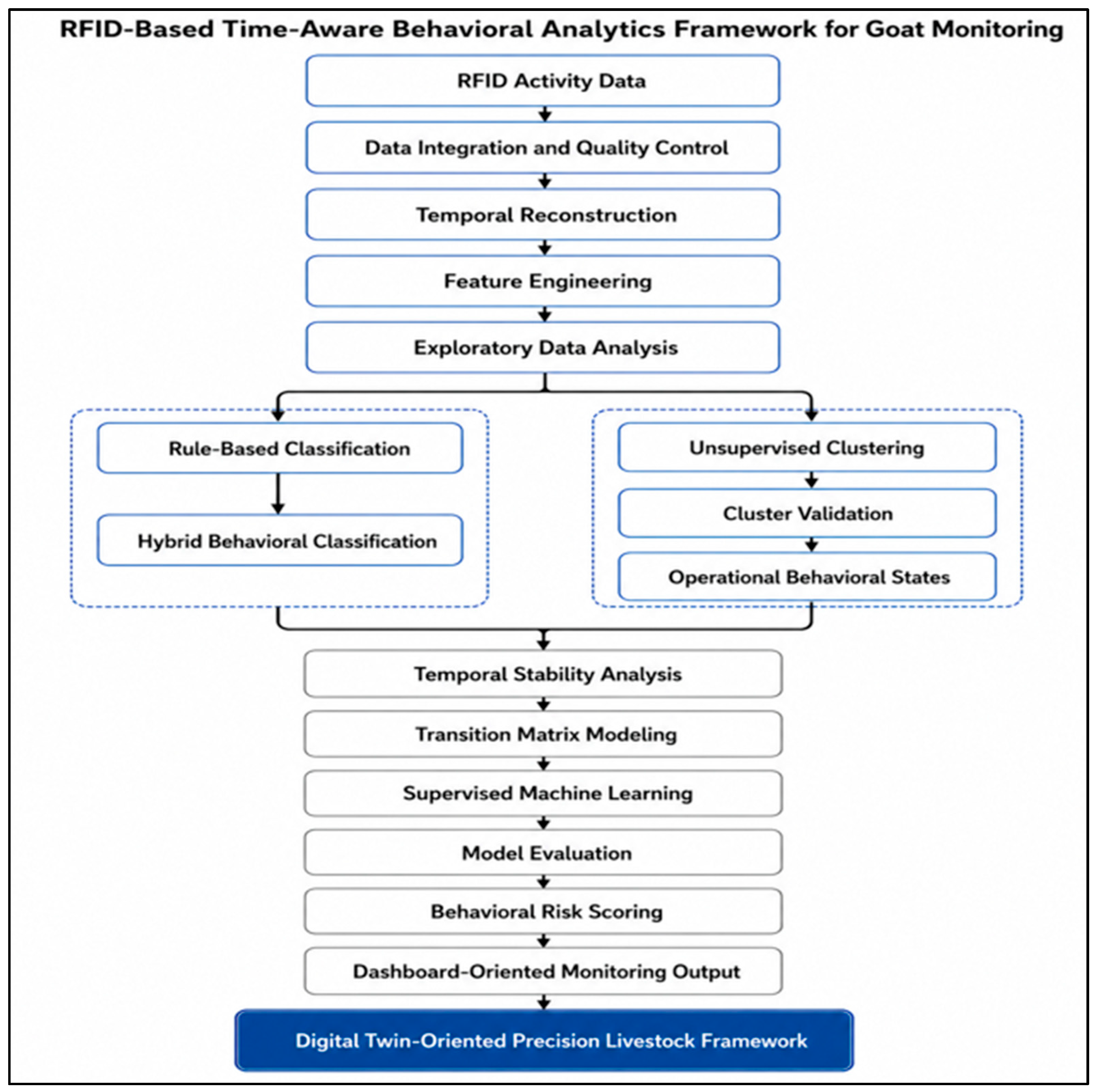
This study developed a time-aware behavioral analytics framework for goats using radio frequency identification (RFID) transponder-linked activity data. The overall objective was to transform raw activity observations into an interpretable monitoring framework capable of identifying latent behavioral states, quantifying temporal transitions, predicting abnormal activity patterns, and supporting a digital twin-oriented architecture for precision livestock management. The full workflow included data integration, temporal reconstruction, feature engineering, exploratory data analysis, hybrid behavioral classification, unsupervised clustering, cluster validation [20], temporal stability analysis, transition matrix modeling, supervised machine learning, risk scoring, and dashboard-oriented deployment. This type of integrated sensing-to-decision pipeline is consistent with current precision livestock farming directions, where sensor data, machine learning, and decision support are combined rather than analyzed as isolated components [1,13,15].

Unless otherwise specified, the equations presented in the methods represent standard mathematical definitions or implementation formulas adapted from time-series preprocessing, clustering, dimensionality reduction, validation metrics, transition matrix analysis, and supervised machine learning. These equations are included to improve transparency and reproducibility rather than to claim novelty for the individual mathematical expressions. The methodological contribution of this study lies in integrating these components into a time-aware RFID-derived goat behavioral monitoring and short-horizon forecasting framework (Figure 1).

2.2. Data Integration and Preprocessing

The RFID activity data were collected through a collaboration with the University of Pretoria, South Africa. The exact farm location is not disclosed for confidentiality reasons. The goats were maintained under a farmer-based production system using standard housing conditions typical of small-scale goat farming. The monitored group consisted of 30 Boer goats managed under a standard grazing system during the spring-to-summer season. RFID-based activity monitoring was conducted using collar-based sensors positioned around the neck of each goat.

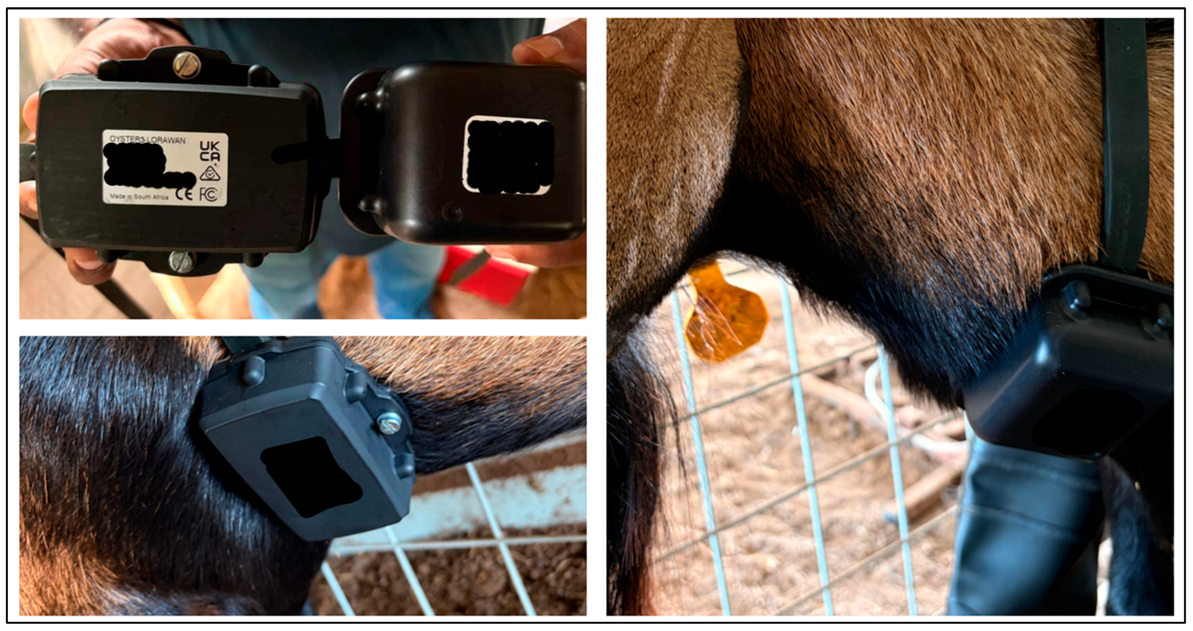
A representative image of the collar-mounted transponder activity device attached to a goat is shown in Figure 2. The device used in this study was the Oyster3 LoRaWAN collar-mounted tracking/transponder unit manufactured by Digital Matter (Johannesburg, South Africa). The device was attached externally to the neck collar and used to generate time-stamped animal-level monitoring records. The dataset used in this study included transponder number, date, time, raw activity score, signal strength, and battery status. The activity score was treated as a raw unitless device-derived activity index rather than a physical time, distance, acceleration, or movement-duration unit. Manufacturer-reported technical specifications for the Oyster3 LoRaWAN system, including LoRaWAN operating regions, GNSS module, supported satellite constellations, power source, battery-life estimates, device dimensions, environmental rating, antenna configuration, and accelerometer capability, are summarized in

Table 2. Technical specifications of the collar-mounted Oyster3 LoRaWAN tracking/transponder system used in the study.

Parameter	Specification
Manufacturer	Digital Matter
Model/device label	Oyster3 LoRaWAN/OYSTER3-LORAWAN
Mounting position in this study	External neck collar attachment
Country of manufacture shown on device label	Made in South Africa
Activity output unit	Raw unitless device-derived activity score
Connectivity/communication mode	LoRaWAN
Supported LoRaWAN frequency regions	868 MHz and 902–928 MHz regions
GNSS module	Sony CXD5605
Supported satellite constellations	Concurrent GPS, GLONASS, Galileo, and BeiDou
Manufacturer-reported location accuracy	Approximately 1 m CEP under ideal conditions
Power source	3 × AA user-replaceable batteries
Supported battery types	Lithium or lithium thionyl chloride batteries
Sleep current	<10 µA
Device dimensions	108 × 86 × 30 mm
Environmental protection rating	IP68 waterproof/dust-resistant housing; IK07 impact rating
Operating temperature range	−30 °C to +60 °C
GPS antenna	Internal
RF antenna	Internal
Motion/activity sensing capability	Built-in 3-axis accelerometer for movement detection

.

Because the dataset came from a single operational management setting, model generalizability across farms, breeds, housing systems, seasons, and environmental conditions should be interpreted cautiously. The final analysis dataset contained 85,890 RFID-derived activity observations collected from 30 goats. Each record included transponder number, date, time, activity level, signal strength, battery life, and derived temporal features, including lag1, lag2, rolling mean, delta, hour, day, month, and day/night indicator.

In the source dataset, activity level was recorded as a raw numeric activity score generated by the RFID/transponder monitoring system. This value was not a time duration and did not represent seconds, minutes, or proportion of time. Because no physical measurement unit was provided with the source data, activity level was treated as a unitless RFID-derived activity index throughout the analysis.

The raw activity levels available in the source dataset were sleep (66,567 observations), abnormal (9804 observations), and normal (9519 observations). After merging source files, records were ordered by goat and timestamp to preserve within-animal temporal continuity for downstream time-aware analyses. The merged dataset was then standardized and converted into an analysis-ready format. During preprocessing, variable names were standardized, duplicate records were removed, fully empty fields were discarded, and missing values were managed to support downstream statistical and machine learning analyses. The original temporal information was stored in separate date and time columns, which were merged into a single datetime field:

$$D{T}_t=D_t+T_t$$

(1)

where $D{T}_t$ is the reconstructed datetime for observation $t$, $D_t$ is the date component, and $T_t$ is the time component. After reconstruction, records were sorted by animal identity and time:

$$\left\{x_{i,t}\right\} \mathrm{ordered} \mathrm{by} (i,t)$$

(2)

where $i$ denotes goat identity (transponder_no) and $t$ denotes temporal sequence. This step was necessary to preserve within-animal temporal continuity and to support lag-based and transition analyses.

2.3. Temporal Feature Engineering

The observation stream was irregularly sampled. In the final lag-ready analysis dataset, all consecutive within-goat sampling intervals had a median of 93 s, an interquartile range of 61–122 s, a mean of 193.99 s, and a maximum of 6,168,262 s, reflecting both short within-session RFID intervals and longer between-session recording gaps. When intervals longer than 6 h were excluded to summarize within-session sampling behavior, the median remained 93 s, the interquartile range was 61–122 s, the mean was 111.76 s, and the maximum was 21,463 s. Therefore, temporal features were calculated from the ordered within-goat observation sequence rather than assuming perfectly uniform sampling. In addition, short-horizon forecasting targets were defined using actual elapsed-time windows of 5 and 10 min rather than fixed row offsets, so that prediction horizons remained time-based despite irregular sampling. A summary of the within-goat sampling interval distribution is provided in Supplementary Table S1.

To capture short-term behavioral dynamics, several temporal features were derived from the activity signal, in which $A_t$ denotes the activity level observed at time $t$, and the first-order change in activity, or delta, is computed as:

$${\Delta }_t=A_t-A_{t-1}$$

(3)

where ${\Delta }_t$ represents the difference between consecutive activity observations. Positive values indicate behavioral escalation, whereas negative values indicate behavioral decline or recovery.

Two lag features were also generated:

$$L_{1,t}=A_{t-1}$$

(4)

$$L_{2,t}=A_{t-2}$$

(5)

where $L_{1,t }$ and $L_{2,t }$ represent first- and second-order behavioral memory, respectively. A three-point rolling average was calculated to summarize local behavioral trend:

$$R{M}_t={\displaystyle \frac{1}{3}}(A_t+A_{t-1}+A_{t-2})$$

(6)

where $R{M}_t$ is the rolling mean at time $t$. Additional time-derived features, including hour, minute, day, month, and a day-versus-night indicator, were extracted from the reconstructed timestamp. The day indicator is defined as:

$$I_{day,t}=\left\{\begin{array}{cc}1,& \mathrm{if} 6\le hou{r}_t\le 19\\ 0,& \mathrm{otherwise}\end{array}\right.$$

(7)

Because the rolling mean was calculated over three consecutive observations rather than a fixed clock-time window, the real-time duration represented by this feature varied across the irregularly sampled data stream. These features were used throughout the clustering, transition, and prediction steps, as they preserved short-term temporal structure that is not captured by raw activity values alone.

2.4. Exploratory Data Analysis

Exploratory data analysis was conducted before formal modeling to characterize the distributional and temporal structure of the goat activity RFID signal. Summary statistics, histograms, state-frequency distributions, hourly activity profiles, day-versus-night comparisons, and delta distributions were examined. This stage was used to determine whether the behavioral stream was dominated by stable baseline activity or by more uniformly distributed movement patterns, and it also informed the development of the hybrid behavioral classification scheme. The exploratory analysis showed that activity was strongly right-skewed and dominated by low-intensity baseline behavior, with relatively rare but distinct high-intensity events.

2.5. Initial Behavioral Thresholds and Hybrid Time-Aware Classification

A preliminary rule-based classification was first defined to assign coarse behavioral categories. The RFID signal activity values from 0 to 40 were interpreted as low-activity or sleep-like states, values from 41 to 99 were interpreted as normal activity, and values greater than or equal to 100 were considered abnormal or high-intensity activity. These categories were not produced from an independently validated behavioral ethogram or clinical diagnostic system. Instead, they represented rule-based activity categories available in the source RFID dataset and were based on static activity-level thresholds. The normal category therefore represented the intermediate activity range defined by this thresholding scheme and should not be interpreted as an individualized biological baseline. Similarly, the abnormal category represented high-intensity activity according to the activity-value threshold and not a confirmed activity-defined abnormal behavior, disease event, or welfare impairment. No synchronized video annotation, physiological measurement, veterinary diagnosis, parasitological record, or clinical welfare scoring system was available to independently ground-truth these labels. Routine daily animal observations were available as general monitoring context, but they were not structured as a formal validation dataset. Therefore, the sleep, normal, and abnormal labels were retained only as descriptive source-data reference categories, while the main analysis focused on activity-derived latent states, transition dynamics, and short-horizon activity-instability forecasting. Because static thresholds do not account for time-of-day context, a hybrid time-aware classification strategy was then used.

For each hour $h$, the mean activity ${\mu }_{h }$ and standard deviation ${\sigma }_h$ were calculated. A time-normalized z-score was then computed for each observation:

$$Z_{t,h}={\displaystyle \frac{A_{t,h}-{\mu }_h}{{\sigma }_h}}$$

(8)

where $A_{t,h}$ is the observed activity at time $t$ during hour $h$, ${\mu }_h$ is the mean activity for hour $h$, and ${\sigma }_h$ is the corresponding standard deviation. This normalization enabled behavioral activity to be interpreted relative to its expected temporal context. The hybrid state definition therefore combined biologically interpretable thresholds with time-specific deviation, allowing elevated activity during biologically active periods to be treated differently from similarly elevated activity during rest-dominant periods. The source dataset contained rule-based activity labels (sleep, normal, and abnormal), which were retained as descriptive reference categories. However, the main analytical framework did not use these labels as the final behavioral ontology. Instead, latent clusters were first identified from continuous activity-derived features, and these clusters were then consolidated into operational behavioral states for transition and prediction analyses. This distinction is important because the reported states reflect data-driven temporal structure rather than the original threshold-based labels alone. These rule-based labels were defined from RFID activity-level thresholds and were cross-checked against routine daily animal observations conducted during animal monitoring. However, they were not independently validated using synchronized video annotation, physiological measurements, or clinical diagnostic records. Therefore, these labels were retained as descriptive source-data reference categories, while the final behavioral states used in the present framework were derived from continuous activity-based temporal features and latent-state modeling.

2.6. Unsupervised Clustering of Behavioral States

To identify latent behavioral regimes without relying exclusively on predefined labels, unsupervised clustering was applied to the standardized behavioral feature set. The main input variables included activity levels, delta, lag terms, and rolling mean. Before clustering, features were standardized as:

$$X_j^{\prime }={\displaystyle \frac{X_j-{\stackrel{-}{X}}_j}{s_j}}$$

(9)

where $X_j$ is the original value of feature $j$, ${\stackrel{-}{X}}_j$ is its mean or average, and $s_j$ is its standard deviation.

2.6.1. K-Means Clustering

K-means clustering was used to partition observations into hard behavioral groups by minimizing the within-cluster sum of squares:

$$J={\displaystyle {\sum }_{i=1}^n}{\displaystyle {\sum }_{k=1}^K}{w}_{ik}\parallel x_i-c_k{\parallel }^2$$

(10)

where $x_i$ is observation $i$; $c_{k }$ is the centroid of cluster $k$; and $w_{ik}=1$ if observation $i$ belongs to cluster $k$, otherwise $w_{ik}=0$.

2.6.2. Fuzzy c-Means Clustering

Because animal behavior often evolves gradually rather than through abrupt jumps, fuzzy c-means clustering was also performed. Unlike K-means, fuzzy c-means assigns each observation partial membership across all clusters. The clustering objective is:

$$J_m={\displaystyle {\sum }_{i=1}^n}{\displaystyle {\sum }_{k=1}^K}{u}_{ik}^m\parallel x_i-c_k{\parallel }^2$$

(11)

where $u_{ik }$ is the membership of observation $i$ in cluster $k$, $m$ is the fuzziness coefficient, and $c_k$ is the cluster centroid. Membership values satisfy:

$${\displaystyle {\sum }_{k=1}^K}{u}_{ik}=1$$

(12)

for each observation $i$. This framework was used to capture mixed-state observations and transitional behavioral regions.

2.7. Cluster Validation and Profiling

To assess whether the identified clusters were meaningful, three internal validation metrics were used: the silhouette coefficient, Davies–Bouldin index, and Dunn index.

The silhouette coefficient for observation $i$ was defined as:

$$s_i={\displaystyle \frac{b_i-a_i}{\mathrm{m}\mathrm{a}\mathrm{x}(a_i,b_i)}}$$

(13)

where $a_i$ is the average intra-cluster distance, and $b_{i }$ is the minimum average distance to the nearest neighboring cluster. Higher silhouette values indicate stronger clustering quality.

The Davies–Bouldin index is defined as:

$$DB={\displaystyle \frac{1}{K}}{\displaystyle {\sum }_{i=1}^K}\underset{j\ne i}{\mathrm{m}\mathrm{a}\mathrm{x}}\left({\displaystyle \frac{S_i+S_j}{M_{ij}}}\right)$$

(14)

where $S_i$ and $S_j$ are within-cluster dispersions, and $M_{ij}$ is the distance between cluster centroids $i$ and $j$. Lower values indicate better separation relative to cluster compactness.

The Dunn index is calculated as:

$$D={\displaystyle \frac{\underset{i\ne j}{\mathrm{m}\mathrm{i}\mathrm{n}} d(C_i,C_j)}{\underset{k}{\mathrm{m}\mathrm{a}\mathrm{x}} \delta (C_k)}}$$

(15)

where $d\left(C_i,C_j\right)$ is the distance between clusters $i$ and $j$, and $\delta \left(C_k\right)$ is the diameter of cluster $k$. Higher Dunn values indicate better clustering structure. After validation, clusters were profiled using mean activity, standard deviation of activity, mean delta, standard deviation of delta, observation count, and percentage of the total dataset. This profiling step enabled clusters to be interpreted biologically as baseline, escalating, recovery, or declining high-intensity states.

To evaluate the robustness of the four-cluster solution, a supplementary clustering sensitivity analysis was performed. K-means was compared with Gaussian Mixture Models, agglomerative hierarchical clustering, DBSCAN, and spectral clustering using the same standardized activity-derived feature set. The algorithms were compared using internal validation metrics, cluster-size distribution, agreement with the primary K-means solution, and interpretability of activity and delta profiles. Because hierarchical and spectral clustering are computationally intensive for the full dataset, these comparisons were conducted as a stratified sensitivity analysis. The final clustering solution was selected based on a combination of quantitative separation, behavioral interpretability, occupancy balance, and suitability for downstream transition and forecasting analyses. Detailed results are provided in Supplementary Tables S8–S10.

2.8. Principal Component Analysis for Visualization

Principal component analysis (PCA) was used to visualize the multivariate behavioral space in two dimensions [21,22,23]. By letting $X$ denote the standardized feature matrix, PCA transforms it into:

$$Z=XW$$

(16)

where $W$ contains the eigenvectors associated with the principal components. PCA was used for visualization rather than inference, allowing the latent-state structure to be interpreted geometrically and helping to assess whether clusters occupied distinct and biologically interpretable regions.

2.9. Behavioral Intensity Index and Boundary-Zone Analysis

To quantify the combined effect of activity magnitude and directional change, a directional behavioral intensity index was calculated as the product of the current activity level and the first-order activity change. Specifically, the index is defined as:

$$BI{I}_t=A_t\times \Delta A_t$$

(17)

where $A_t$ is the RFID-derived activity level at time $t$, and $\Delta A_t=A_t-A_{t-1}$ is the change in activity relative to the previous observation from the same goat. Positive values indicate increases in activity, especially when high current activity follows lower previous activity. Negative values indicate declines in activity, especially when current activity remains elevated but is lower than the previous observation. Values near zero indicate stable low activity or little change between consecutive observations. Therefore, this index was used as a descriptive activity-change metric rather than as a validated biological or clinical marker.

Because the behavioral intensity index was calculated as the product of activity level and activity change, it was expected to emphasize observations where high current activity coincided with abrupt escalation. This multiplicative form was used as a descriptive activity-escalation metric rather than as a validated biological or clinical marker. However, because multiplicative indices can be sensitive to extreme observations, a robust sensitivity analysis was also performed using winsorized, robust-scaled, and signed-log-transformed versions of the index. These robust versions were used to determine whether the interpretation of episodic activity escalation was retained after reducing the influence of outliers.

Boundary-zone analysis was then performed to identify observations located between stable and unstable behavioral states. In parallel, fuzzy c-means membership values were used to quantify uncertainty. For each observation, the maximum membership value was used as a confidence score:

$$Con{f}_i=\underset{k}{\mathrm{m}\mathrm{a}\mathrm{x}}(u_{ik})$$

(18)

where $Con{f}_i$ is the confidence of observation $i$ belonging to its most likely cluster. Lower confidence values were interpreted as mixed or transitional behavioral points. Observations with maximum fuzzy-membership confidence below 0.60 were classified as uncertain or mixed-state observations. These regions were particularly important for identifying pretransition states relevant to early warning.

Boundary-zone and fuzzy-uncertain observations were also prospectively evaluated to determine whether they were more likely to precede future high-activity/non-baseline states. Future event rates were compared between boundary-zone and non-boundary observations and between fuzzy-uncertain and certain observations within 5 min and 10 min forecasting windows. Risk ratios and odds ratios were calculated to quantify the association between uncertainty status and subsequent high-activity/non-baseline state onset.

2.10. Temporal Stability and Individual-Level Behavioral Profiling

Temporal stability was assessed by measuring how long each goat remained in the same cluster or state before transitioning. After sorting records by transponder_number and datetime, changes in state assignment were used to define contiguous behavioral segments, and segment lengths were summarized to quantify mean duration, median duration, and extreme persistence.

At the individual level, the proportion of time each goat spent in each cluster was also calculated:

$$P_{i,k}={\displaystyle \frac{n_{i,k}}{{\displaystyle {\sum }_{k=1}^K}{n}_{i,k}}}$$

(19)

where $P_{i,k}$ is the proportion of observations for goat $i$ in cluster $k$, and $n_{i,k }$ is the count of observations assigned to that cluster. This enabled the identification of animal-specific behavioral profiles and goats with elevated occupancy in non-baseline states.

2.11. Transition Matrix and State-Dynamics Analysis

After four latent clusters were identified, they were consolidated into three operational states for transition and forecasting analyses to simplify state-dynamics interpretation and reduce redundancy between clusters with similar high-activity profiles. Cluster 0 was assigned to the baseline low-activity state because it represented the dominant low-activity pattern. Cluster 2 was assigned to the intermediate or recovery-transition state because it showed moderate activity with negative delta values. Clusters 1 and 3 were combined into a high-activity/non-baseline state because both showed high mean activity values and represented elevated activity regimes, although Cluster 1 reflected increasing activity and Cluster 3 reflected declining high-intensity activity. This consolidation was used only for operational transition modeling and forecasting; the original four-cluster profiles were retained and reported separately to preserve the unsupervised clustering results. To model behavioral evolution over time, a first-order transition matrix was constructed from consecutive state assignments within each goat. The transition probability from state $i$ to state $j$ was defined as:

$$P_{ij}={\displaystyle \frac{n_{ij}}{\sum _j{n}_{ij}}}$$

(20)

where $n_{ij }$ is the number of observed transitions from state $i$ to state $j$. Each row of the transition matrix was normalized so that transition probabilities were summed or added to one.

From this matrix, state stability was defined as the self-transition probability:

$$S_i=P_{ii}$$

(21)

Volatility was defined as:

$$V_i=1-P_{ii}$$

(22)

and transition entropy was calculated as:

$$H_i=-{\sum }_j{P}_{ij} \mathrm{l}\mathrm{n}(P_{ij})$$

(23)

where $H_i$ quantifies uncertainty in the outgoing transition distribution for state $i$. These metrics were used to distinguish persistent baseline states from volatile or high-activity or non-baseline states.

To evaluate whether the first-order transition assumption was sufficient, a supplementary higher-order temporal-dependency analysis was also performed. First-order and second-order Markov state-history models were compared for next-state prediction using accuracy, balanced accuracy, macro-F1, and log loss. In addition, state-duration summaries were calculated as a semi-Markov diagnostic to assess whether state residence time varied across behavioral states. These analyses were used to determine whether longer temporal memory or duration-dependent state structure may improve behavioral state prediction beyond the first-order transition matrix.

2.12. Supervised Machine Learning Modeling and Nested Cross-Validation for High Activity/Non-Baseline State Prediction

To reduce optimistic bias and prevent information leakage, supervised modeling was conducted using nested validation schemes rather than a single random train–test split. For concurrent activity-defined non-baseline state classification, grouped nested cross-validation was used, with transponder numbers defining the grouping structure. In this design, outer folds were reserved for performance estimation, whereas inner folds were used for model selection, hyperparameter tuning, and all preprocessing steps. For forecasting analyses, nested time-blocked validation was used to preserve temporal order and prevent future information from entering model development. In the forecasting framework, the first 70% of each goat’s ordered observations were used for model development and the final 30% were reserved for testing, while inner time-series splits were used for tuning within the training portion only.

Predictor variables included activity level, signal strength, battery life, lagged activity values, rolling mean, delta, hour, day, month, day/night indicator, and elapsed time since the previous observation. Preprocessing was embedded within the modeling pipeline and included median imputation and standardization. Class imbalance was handled using model class weights rather than synthetic oversampling. Logistic regression and Random Forest were used for both concurrent classification and short-horizon forecasting analyses. Model performance was assessed using area under the receiver operating characteristic curve (AUC), average precision or precision–recall area under the curve (AP), precision, recall, F1-score, and Brier score.

To provide a more complete evaluation under class imbalance, additional metrics were calculated, including balanced accuracy, Matthews Correlation Coefficient, Cohen’s Kappa, specificity, and confusion matrix components. Bootstrap resampling was used to estimate confidence intervals for key model-performance metrics and to compare Random Forest with logistic regression using paired bootstrap differences. Calibration was assessed using calibration curves, calibration intercept, calibration slope, and Brier score. Decision curve analysis was also performed to evaluate model net benefit across clinically relevant risk-threshold ranges.

For the main nested time-blocked forecasting analysis, two models were evaluated: logistic regression and Random Forest. Logistic regression was implemented with max_iter = 3000 and class_weight = balanced. The regularization parameter was tuned using C = 0.1, 1.0, and 5.0. Random Forest was implemented with random_state = 42, class_weight = balanced_subsample, and n_jobs = -1. The Random Forest tuning grid included n_estimators = 150 or 250; max_depth = 8, 12, or none; and min_samples_leaf = 1 or 5. GridSearchCV was used for model selection with ROC-AUC as the scoring metric. Grouped nested cross-validation used five outer GroupKFold splits and three inner GroupKFold splits for concurrent classification, while the forecasting analysis used a 70/30 time-blocked outer split within each goat and three inner TimeSeriesSplit folds. For the concurrent classification analysis reported in the Supplementary Materials, SVM was implemented with probability = true and random_state = 42; KNN used n_neighbors = 5; BPNN/MLP used hidden_layer_sizes = (64, 32), max_iter = 300, and random_state = 42; and Random Forest used n_estimators = 100 and random_state = 42.

Short-Horizon Forecasting of Future High-Activity/Non-Baseline State Onset

To test whether the framework supported genuine prospective prediction rather than concurrent classification alone, future activity-defined high-activity/non-baseline targets were defined within each goat’s ordered time series. For each observation at time t, binary forecasting targets indicated whether a high-activity/non-baseline state occurred within the next 5 min or within the next 10 min. Because the observation stream was irregularly sampled, forecasting horizons were defined in time units rather than row offsets. All forecasting predictors were restricted to information available at or before time t.

To evaluate whether the temporal feature forecasting framework provided value beyond simple rule-based approaches, additional baseline comparisons were performed. The persistence baseline used the current activity-defined state as the prediction for future high-activity occurrence, while the threshold baseline classified observations as high activity when the current activity value was ≥100. A no-event baseline was also included for reference. For the baseline comparison, Random Forest models were fitted using a fixed random seed and class-weighted learning; model settings were kept consistent across the 5 min and 10 min forecasting horizons to support reproducibility. These baselines were compared with logistic regression and Random Forest models trained using activity-derived temporal features only. Model performance was evaluated on the held-out time-blocked test set.

2.13. Risk Scoring, Alerts, and Proof-of-Concept Behavioral-Risk Proxy Layer

A continuous risk score was generated for each observation using model probability outputs or normalized behavioral metrics, depending on the stage of the pipeline. When probability-based prediction was available, risk at time $t$ is defined as:

$$R_t=\mathrm{P}\mathrm{r}(Y_t=1\mid X_t)$$

(24)

where $R_t$ is the estimated probability of high-activity or non-baseline states, $Y_{t }$ is the activity-defined non-baseline outcome, and $X_t$ is the feature vector. These risk values were then used to define risk-based alerts, particularly when high-risk scores occurred within intermediate states that tended to precede transitions into high-activity/non-baseline states. A proof-of-concept behavioral-risk proxy layer was also added by combining elevated risk scores with high-activity/non-baseline state assignments. This component was intended as a proof-of-concept extension toward behavior-oriented monitoring rather than as a clinically validated disease classification module.

2.14. Operational Digital Twin Architecture for Animal-Level Behavioral Intelligence

To support time-aware prediction, short behavioral sequences were constructed from consecutive observations for each goat. Sequence-based modeling used recent behavioral history rather than a single observation to estimate future high-activity or non-baseline states, thereby capturing state evolution over time. In parallel, a digital twin-oriented framework was developed in which each goat was represented by a continuously updated virtual behavioral profile consisting of current state, temporal trajectory, risk score, alert condition, and recent transition history. This framework is described as digital twin-oriented because it links sensor-derived activity data to an updated animal-level virtual representation for monitoring and decision support. However, the present implementation should be interpreted as an early-stage or partial digital twin architecture, not a fully bi-directional digital twin, because it does not yet include simulation of alternative management actions, automated intervention, or closed-loop feedback from additional physiological, clinical, parasitological, or environmental data streams.

2.15. Prototype Dashboard Visualization and Future Deployment Architecture

A prototype dashboard was implemented in Google Colab using Gradio (Version 6.20.0) and interactive plotting libraries. This implementation was used as a proof-of-concept visualization interface rather than as a production-level continuous monitoring system. The dashboard displayed per-animal activity trajectories, risk-score visualization, behavioral state distributions, and alert outputs to demonstrate how the analytical workflow could be communicated to users.

Because Google Colab is a development environment and Gradio provides a lightweight interface rather than a robust farm-scale infrastructure, the present dashboard should be interpreted as a static prototype visualizer. A scalable deployment system would require a dedicated architecture for real-time or near-real-time processing. In such a system, RFID readers would transmit activity data to a local edge device or cloud ingestion layer. Preprocessing would standardize timestamps, calculate lag features, rolling means, activity change, and elapsed-time variables, and then pass these features to a model-inference service. Prediction outputs, state assignments, risk scores, and alert labels would be stored in a persistent database and displayed through a hosted dashboard. For field deployment, edge computing devices, such as local gateways, Raspberry Pi, NVIDIA Jetson, or farm servers, could support low-latency processing when internet connectivity is limited, while cloud services could support centralized storage, multi-farm monitoring, model updating, and alert delivery through email, SMS, or mobile applications. Future work should evaluate this architecture prospectively under farm conditions with real-time data streams, alert-threshold calibration, system uptime monitoring, and user-facing performance assessment.

2.16. Computational Environment

All preprocessing, feature engineering, clustering, validation, transition analysis, machine learning, and dashboard development were conducted in Python within a Google Colab environment. All analyses were conducted in a Python 3.12 Google Colab environment. The main Python packages used were numpy 2.0.2, pandas 2.2.2, scikit-learn 1.6.1, matplotlib 3.10.0, seaborn 0.13.2, scipy 1.16.3, plotly 5.24.1, gradio 5.50.0, and cupy-cuda11x 13.6.0. Detailed package versions and model settings are provided as Supplementary Tables S6 and S7 to support reproducibility.

3. Results

3.1. Behavioral State Structure of Goat Activity Data

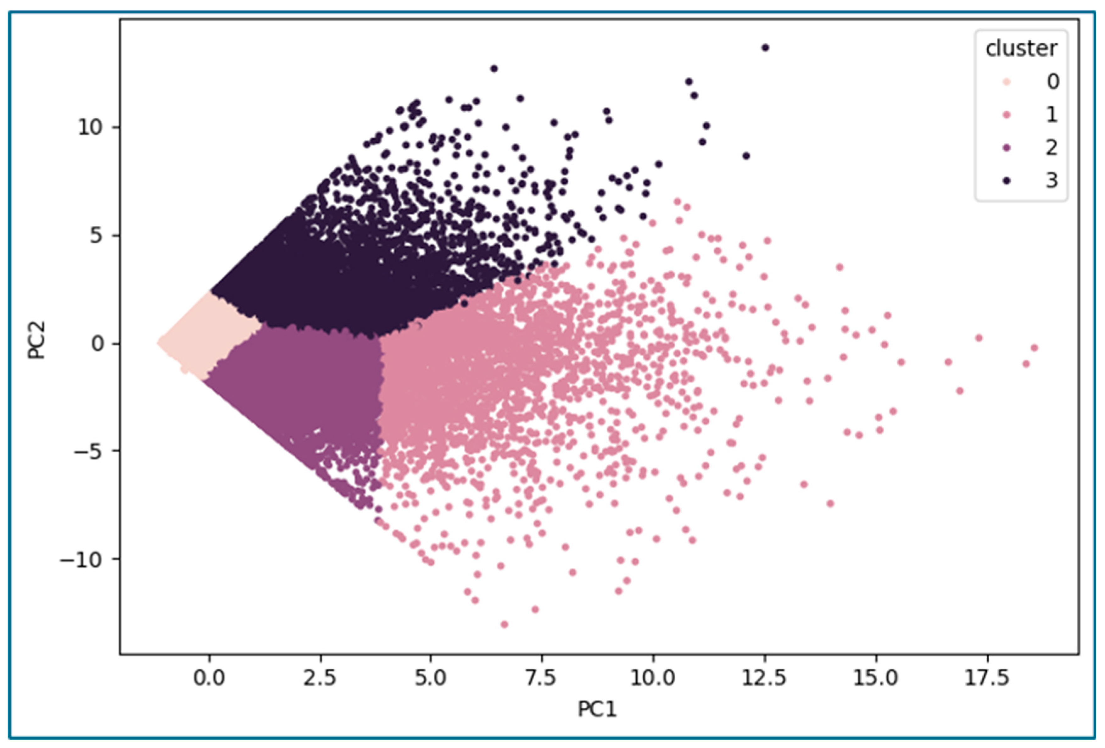
Unsupervised analysis showed clear structure in the goat activity data, with observations distributed across four clusters in the PCA space (Figure 3). The projection showed a wedge-shaped distribution, with a dense concentration of observations at lower PC1 values and broader dispersion as PC1 increased. Cluster separation was visible in the PCA plot, with Cluster 0 concentrated near the origin, Cluster 1 extending mainly toward higher positive PC1 values, Cluster 2 occupying the lower central region, and Cluster 3 distributed primarily in the upper region of the plot.

Cluster profiling identified four distinct behavioral clusters (

Table 3. Cluster-level behavioral profiles derived from goat RFID activity data. Activity values are reported as raw unitless RFID-derived activity scores rather than time-based measurements.

Cluster	Mean Activity Score	SD Activity Score	Mean Delta	SD Delta	n	%
0	9.82	20.08	2.15	20.35	66,892	77.88
1	188.53	84.05	128.05	81.14	5978	6.96
2	46.30	43.07	−67.44	66.40	9935	11.57
3	184.44	107.98	−77.71	122.47	3085	3.59

). Mean delta, defined as the average change in activity relative to the previous observation, differed across clusters. Cluster 0 was the largest group, containing 66,892 observations (77.88%), and had the lowest mean activity score (9.82) and a mean delta of 2.15. Cluster 1 included 5978 observations (6.96%) and had the highest mean activity score (188.53), together with the highest positive mean delta (128.05). Cluster 2 contained 9935 observations (11.57%) and showed moderate mean activity score (46.30) with a negative mean delta (−67.44). Cluster 3 was the smallest group, with 3085 observations (3.59%), and had a high mean activity score (184.44) and a negative mean delta (−77.71). Variation also differed among clusters. Cluster 0 showed the lowest activity variability (SD = 20.08), whereas Cluster 3 showed the highest variability in both activity score (SD = 107.98) and delta (SD = 122.47). Cluster 1 also showed high dispersion, with SD values of 84.05 for activity score and 81.14 for delta.

A supplementary clustering sensitivity analysis supported the use of the four-cluster K-means solution. In the stratified comparison, K-means produced a silhouette coefficient of 0.662 and a Davies–Bouldin index of 0.936, while agglomerative hierarchical clustering produced a similar structure with a silhouette coefficient of 0.635 and a Davies–Bouldin index of 1.002. Gaussian Mixture Models and spectral clustering showed weaker cluster separation and lower agreement with the primary K-means solution. DBSCAN identified only two non-noise clusters, assigned 17.55% of observations as noise, and placed 99.27% of non-noise observations into one dominant cluster, which limited its behavioral interpretability. Although the two-cluster K-means solution produced the highest silhouette value, it collapsed the behavioral structure into a broad low-versus-high activity split. Therefore, the four-cluster solution was retained because it preserved more interpretable baseline, increasing high-activity, moderate/recovery, and declining high-activity profiles. Detailed clustering sensitivity results are provided in Supplementary Tables S8–S10.

The first two principal components preserved most of the standardized behavioral feature-space information. PC1 explained 62.37% of the variance, while PC2 explained 28.51%, giving a cumulative explained variance of 90.89%. Therefore, the two-dimensional PCA projection was considered appropriate for visualizing the major cluster structure. Internal validation metrics further supported the presence of structured but partially overlapping behavioral clusters. The four-cluster K-means solution produced a silhouette coefficient of 0.6458, a Davies–Bouldin index of 1.0208, and a Dunn index of 0.1279. The silhouette coefficient indicated moderate separation among clusters, while the Davies–Bouldin index suggested acceptable but incomplete compactness and separation. The relatively low Dunn index indicated that some overlap remained among clusters, which is expected in animal activity data because behavioral states may shift gradually rather than through sharply separated boundaries. Overall, these validation results supported the use of the four-cluster solution for exploratory latent-state discovery while also justifying the later fuzzy uncertainty and boundary-zone analyses.

3.2. Behavioral Intensity Distribution and Evidence of Episodic High-Risk Events

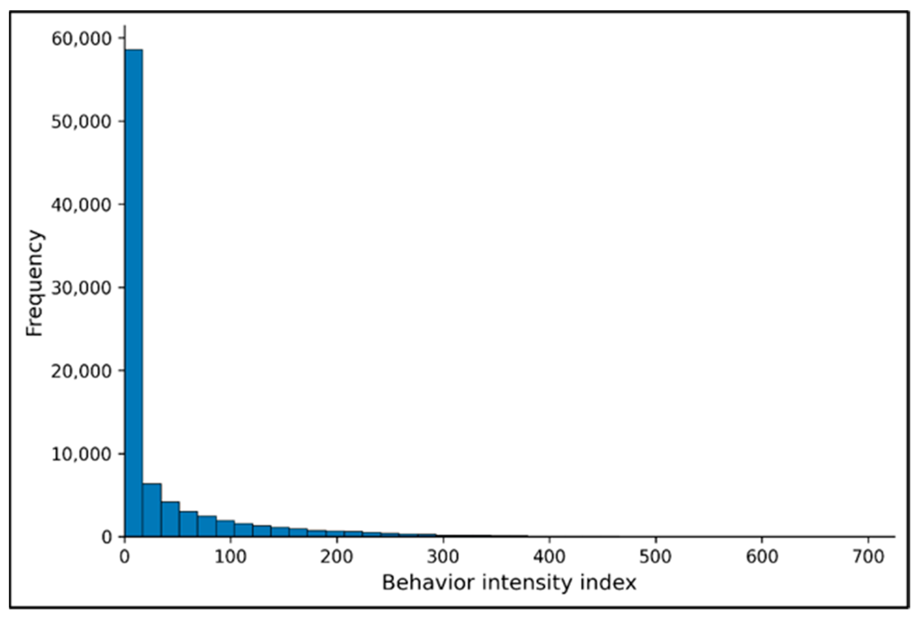
The behavior intensity index showed a strongly right-skewed distribution (Figure 4). Most observations were concentrated near zero, with relatively few observations extending into large positive values and a smaller number extending into negative values. The median was zero, the 75th percentile was 42, the mean was 1857.63, and the standard deviation was 13,145.45. The observed values ranged from −97,128 to 476,100. These extreme values resulted from the multiplicative structure of the index. The maximum value occurred when activity increased sharply from 0 to 690, producing a delta of 690 and an index value of 476,100. The minimum value occurred when activity declined from 626 to 284, producing a delta of −342 and an index value of −97,128. Thus, the long right tail reflects episodic sharp increases in activity, whereas the negative tail reflects sharp declines after high activity. These patterns may represent abrupt activity bursts, recovery after intense movement, sensor-detected movement fluctuations, or short-term behavioral transitions; however, because no synchronized video or physiological validation was available, the index should be interpreted as an activity-derived descriptive metric rather than a direct biological state indicator.

A robust sensitivity analysis was performed to evaluate whether the behavioral intensity interpretation was driven only by extreme values. The 1st–99th percentile winsorized index reduced the maximum value from 476,100 to 52,508.58 while preserving the rank structure of the original index. The winsorized index remained almost perfectly rank-correlated with the original index, and the robust-scaled index also retained a strong rank correlation with the original formulation. Top-decile values of the original, winsorized, robust-scaled, and signed-log-transformed indices were strongly associated with future high-activity/non-baseline states within both 5 min and 10 min horizons. For the original index, top-decile observations had a 5 min future event rate of 55.6% compared with 14.3% for other observations, corresponding to an odds ratio of 7.52. For the 10 min horizon, the top-decile event rate was 67.1% compared with 21.7% for other observations, corresponding to an odds ratio of 7.38. These results indicate that the behavioral intensity signal was not only an artifact of extreme outliers. Detailed sensitivity results are provided in Supplementary Tables S11 and S12.

The histogram showed a large peak near zero and a long right tail, indicating that low intensity values were the most common in the dataset, whereas high intensity values occurred much less frequently. Negative values were also present but were less frequent than the positive extreme values. Overall, the distribution indicates that the behavior intensity index was dominated by low values, with a limited number of extreme observations on both sides of the distribution.

3.3. Boundary Regions and Uncertain Observations

Boundary-zone analysis identified 6274 observations (7.30%) in the transition region between stable and unstable behavioral regimes. In addition, fuzzy clustering classified 21.42% of all observations as uncertain points based on low maximum membership confidence. These results show that a measurable portion of the dataset was in intermediate or mixed-state regions rather than in clearly separated clusters. The dominant cluster percentage, boundary-zone percentage, and fuzzy-uncertainty percentage should not be summed because they describe different and partially overlapping analytical outputs. The dominant cluster percentage represents hard K-means cluster assignment, whereas boundary-zone observations were identified from the transition region between stable and unstable activity regimes, and fuzzy-uncertain observations were identified from low maximum membership confidence in the fuzzy clustering analysis. Therefore, an observation could belong to the dominant hard cluster while also being near a boundary or having lower fuzzy-membership confidence.

Predictive validation showed that boundary-zone and fuzzy-uncertain observations were more likely to precede future high-activity/non-baseline states. For the 5 min horizon, boundary-zone observations had a future event rate of 58.92%, compared with 15.19% for non-boundary observations, corresponding to an odds ratio of 8.01. For the 10 min horizon, boundary-zone observations had a future event rate of 71.64%, compared with 22.63% for non-boundary observations, corresponding to an odds ratio of 8.63. Fuzzy-uncertain observations showed a similar pattern. For the 5 min horizon, fuzzy-uncertain observations had a future event rate of 45.00%, compared with 11.14% for certain observations, corresponding to an odds ratio of 6.53. For the 10 min horizon, fuzzy-uncertain observations had a future event rate of 57.09%, compared with 17.80% for certain observations, corresponding to an odds ratio of 6.14. These results support the practical value of boundary-zone and fuzzy-uncertainty metrics as early-warning indicators of future activity-defined high-activity/non-baseline states. Detailed results are provided in Supplementary Table S13.

3.4. Temporal Stability and Persistence of Goat Behavioral Regimes

Temporal stability analysis showed that behavioral states included many short runs together with a smaller number of highly persistent episodes. Across all animals and state segments, the mean duration was 5.30 observations, the median duration was 1 observation, and the maximum duration was 3205 observations.

All 30 goats were dominated by Cluster 0 (low activity), indicating that this was the most frequent state for every individual. However, between-animal variation was observed in the proportion of time spent outside the baseline cluster. When Clusters 1, 2, and 3 were combined as non-baseline states, the numerically highest proportions were observed for transponders 40011301504 (40.71%), 40011301520 (38.96%), 40011301534 (37.92%), 40011301539 (37.86%), and 40011301551 (35.92%). These results indicate that, although Cluster 0 was the dominant state across all goats, the frequency of non-baseline states varied among individuals.

3.5. Dynamic State Transitions and the Emergence of High-Activity or Non-Baseline States

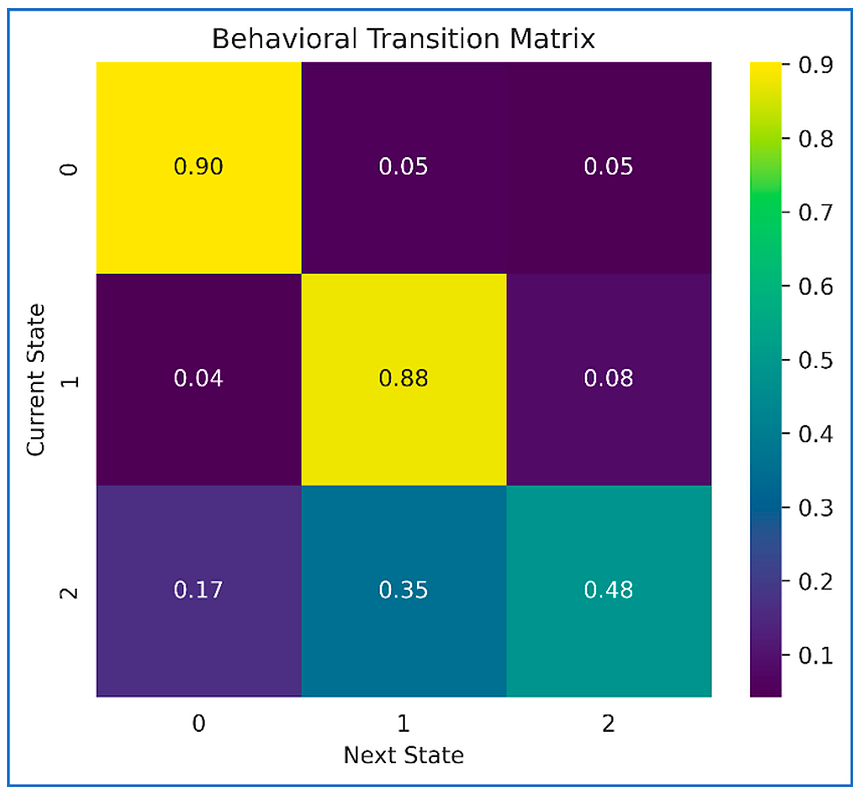
Although the unsupervised clustering initially identified four clusters, these were consolidated into three behavioral states for the transition analysis based on overall activity structure and time-aware behavioral context; therefore, the transition framework includes States 0–2 only. Specifically, Cluster 0 was mapped to State 0, Cluster 2 was mapped to State 1, and Clusters 1 and 3 were combined into State 2 for the three-state transition analysis. Transition analysis showed clear differences in persistence among the three behavioral states (Figure 5;

Table 4. Transition probabilities and state-level temporal metrics of the three-state behavioral system.

Current State	Next 0	Next 1	Next 2
0	0.903	0.051	0.046
1	0.043	0.877	0.080
2	0.165	0.350	0.485
State	Stability	Volatility	Entropy
0	0.903	0.097	0.385
1	0.877	0.123	0.452
2	0.485	0.515	1.016

). State 0 had the highest self-transition probability (0.903), followed by State 1 (0.877), whereas State 2 had a lower self-transition probability (0.485). These values indicate that States 0 and 1 were more persistent across consecutive observations, while State 2 was less persistent.

Transitions from State 0 occurred mainly back to State 0, with smaller probabilities of moving to State 1 (0.051) or State 2 (0.046). Similarly, State 1 most often remained in State 1, with lower probabilities of transitioning to State 0 (0.043) or State 2 (0.080). In contrast, State 2 showed greater redistribution across states, with transition probabilities of 0.165 to State 0, 0.350 to State 1, and 0.485 remaining in State 2.

State-level temporal metrics showed the same pattern. State 0 had stability of 0.903, volatility of 0.097, and entropy of 0.385. State 1 had stability of 0.877, volatility of 0.123, and entropy of 0.452. State 2 showed lower stability (0.485), higher volatility (0.515), and the highest entropy (1.016). Overall, States 0 and 1 were more stable and predictable, whereas State 2 showed greater variability and lower persistence.

A supplementary higher-order temporal-dependency analysis showed that including longer state history improved next-state prediction compared with the first-order transition assumption. The first-order Markov model achieved an accuracy of 0.857, balanced accuracy of 0.591, macro-F1 of 0.508, and log loss of 0.355. The second-order Markov model improved performance, with accuracy of 0.891, balanced accuracy of 0.630, macro-F1 of 0.673, and log loss of 0.336. These results indicate that the first-order transition matrix provided an interpretable summary of immediate state persistence and transition direction, but longer temporal memory may capture additional behavioral structure. Detailed results are provided in Supplementary Table S15.

3.6. Concurrent Classification of Activity-Defined States

Concurrent classification was performed as a secondary analysis to evaluate the internal separability of the activity-defined behavioral state system. Because the non-baseline target was derived from the same RFID activity stream used to construct predictor variables such as delta, lagged activity, and rolling mean, this analysis was not interpreted as independent biological prediction. Detailed concurrent classification results, including model-level performance metrics and confusion matrix summaries, are provided in Supplementary Table S5. The main predictive evaluation of the framework is therefore based on the nested time-blocked forecasting analysis presented below.

3.7. Short-Horizon Forecasting of Future High-Activity/Non-Baseline State Onset

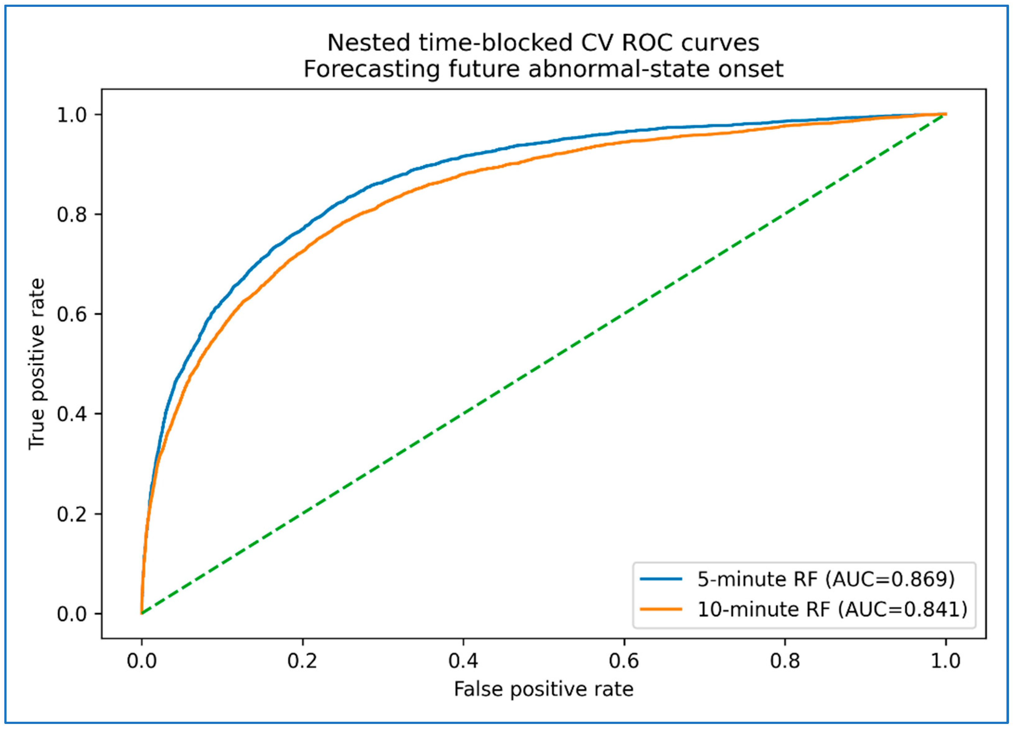
Short-horizon forecasting analyses were performed to evaluate whether future high-activity/non-baseline state onset could be forecasted under time-respecting validation. Using nested time-blocked cross-validation, Random Forest achieved an AUC of 0.869 for forecasting high-activity/non-baseline state onset within the next 5 min and an AUC of 0.841 for the 10 min horizon (Figure 6). Precision–recall analysis showed average precision values of 0.612 for the 5 min horizon and 0.670 for the 10 min horizon (Figure S2). These results indicate that the activity stream contained useful information for short-horizon forecasting of prospective activity instability beyond concurrent state classification. Forecasting horizon coverage was high in the lag-ready dataset, with future observations available within the 5 min horizon for 83,445 of 85,890 records (97.15%) and within the 10 min horizon for 85,444 records (99.48%; Supplementary Table S4).

Forecasting performance declined modestly from the 5 min to the 10 min horizon in ROC space, whereas precision–recall performance remained strong and was slightly higher at the 10 min horizon. This pattern likely reflects the higher event prevalence at the 10 min horizon. Because the 10 min window provided a longer opportunity for a future high-activity/non-baseline event to occur, the event rate increased from 19.53% at 5 min to 27.78% at 10 min (Supplementary Table S4). Average precision is sensitive to event prevalence and ranking performance among positive cases, whereas ROC-AUC summarizes discrimination across both positive and negative classes. Therefore, a modest decline in ROC-AUC together with a higher average precision at the 10 min horizon is not contradictory but reflects differences between ROC- and precision–recall-based evaluation under changing event prevalence. Overall, these findings support the feasibility of short-horizon forecasting of future activity instability within this dataset from recent behavioral dynamics, while also showing that prospective prediction is more difficult than concurrent high-activity/non-baseline state discrimination. A summary comparison of nested validation performance across concurrent classification and forecasting tasks is provided in Figure S3. Baseline comparisons showed that temporal feature models provided added value beyond simple rule-based approaches (Supplementary Table S2). For the 5 min horizon, the persistence and threshold baselines produced an F1-score of 0.506 and AUC of 0.682, whereas Random Forest using activity-derived temporal features achieved an F1-score of 0.586 and AUC of 0.865. For the 10 min horizon, the persistence and threshold baselines produced an F1-score of 0.439 and AUC of 0.639, whereas Random Forest achieved an F1-score of 0.617 and AUC of 0.839. These results indicate that recent temporal features improved short-horizon prediction compared with current-state or threshold-only rules. Random Forest feature-importance analysis showed that prediction performance was driven mainly by rolling mean, current activity level, lagged activity, elapsed time, delta, signal strength, and hour of day. The full feature-importance ranking is provided in Supplementary Table S3. This indicates that forecasting was influenced by both recent activity history and short-term temporal context rather than by current activity magnitude alone.

Expanded model evaluation confirmed that the forecasting models retained useful discrimination under class imbalance. For 5 min forecasting, Random Forest achieved an AUC of 0.868, average precision of 0.609, balanced accuracy of 0.783, MCC of 0.472, Cohen’s Kappa of 0.451, and Brier score of 0.130. Logistic regression showed similar but slightly lower discrimination, with AUC of 0.859, average precision of 0.600, balanced accuracy of 0.777, MCC of 0.477, Cohen’s Kappa of 0.463, and Brier score of 0.157. For 10 min forecasting, Random Forest achieved an AUC of 0.840, average precision of 0.668, balanced accuracy of 0.763, MCC of 0.478, Cohen’s Kappa of 0.467, and Brier score of 0.154, while logistic regression achieved an AUC of 0.824, average precision of 0.656, balanced accuracy of 0.752, MCC of 0.482, Cohen’s Kappa of 0.480, and Brier score of 0.173. Bootstrap comparison showed that Random Forest had statistically higher AUC than logistic regression at both horizons, although differences in MCC and Cohen’s Kappa were small. Calibration and decision curve analyses are provided in the supplementary materials.

3.8. Digital Twin Implementation and Animal-Level Monitoring

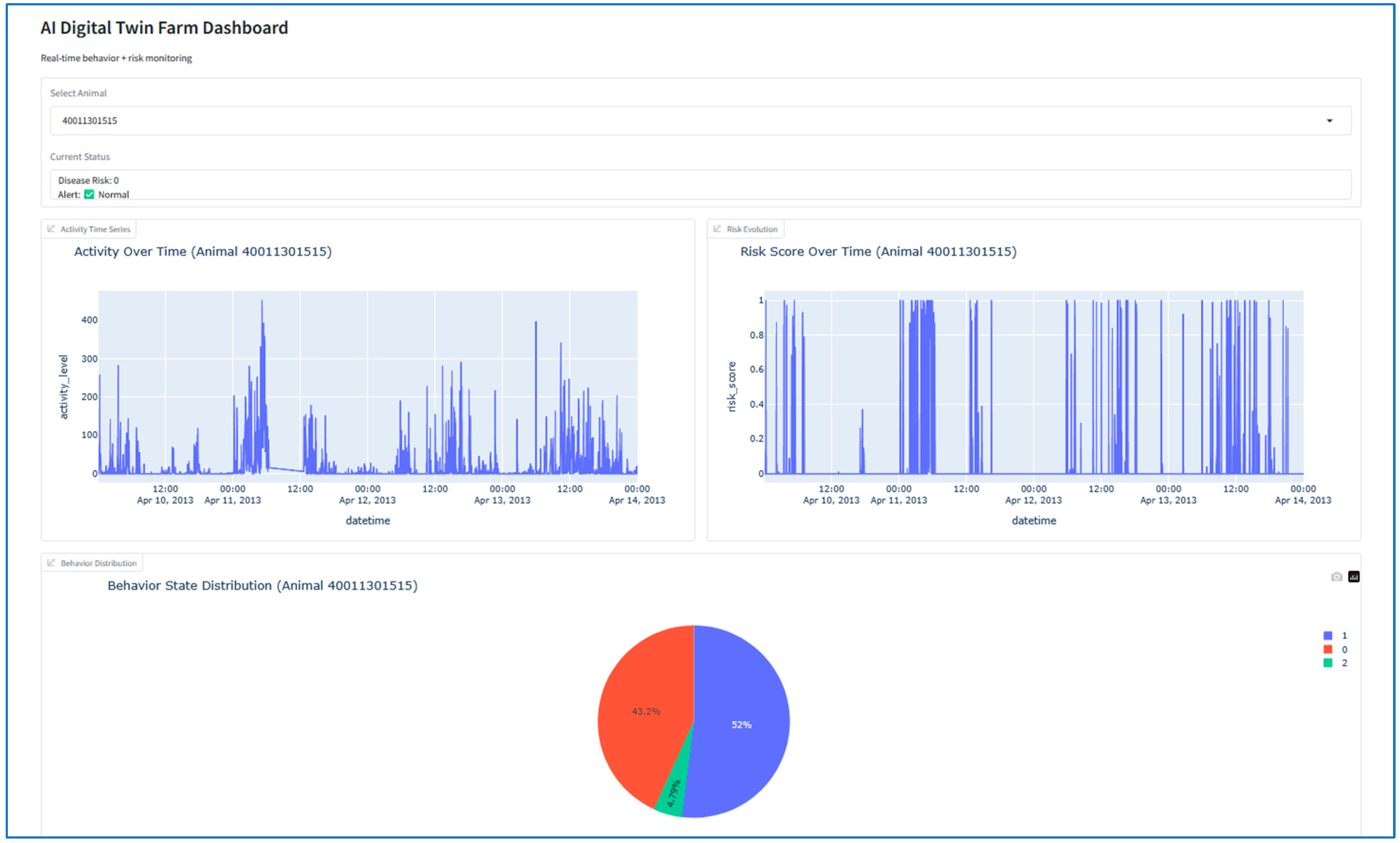
The predictive outputs were incorporated into a digital twin-oriented monitoring framework that combined behavioral states, risk scores, alert labels, and animal-level visualization (Figure 7). The final digital twin dataset contained 85,890 observations from 30 goats, with each record linked to transponder number, timestamp, behavioral state, risk score, alert condition, and behavioral-risk proxy. Across the full dataset, State 1 was the most frequent state (41,684 observations), followed by State 0 (34,665 observations) and State 2 (9541 observations). This ordering differs from the cluster-level results because the final digital twin states were derived from the integrated three-state operational framework rather than by direct one-to-one renumbering of the original four clusters.

The mean risk score across all observations was 0.111, with a maximum value of 1.00. Alert classification labeled 76,347 observations as normal and 9541 observations as abnormal, with a small number classified as early-warning records. The highest mean risk scores were observed for transponders 40011301504 (0.265), 40011301520 (0.221), 40011301534 (0.208), 40011301539 (0.208), and 40011301542 (0.183).

Figure 7 shows an example dashboard output for the individual animal with the transponder number 40011301515. The display included activity over time, risk score over time, and behavioral state distribution. For this animal, the state distribution consisted of 52.0% for State 1, 43.2% for State 0, and 4.8% for State 2. The risk trace showed multiple short duration increases across the monitoring period.

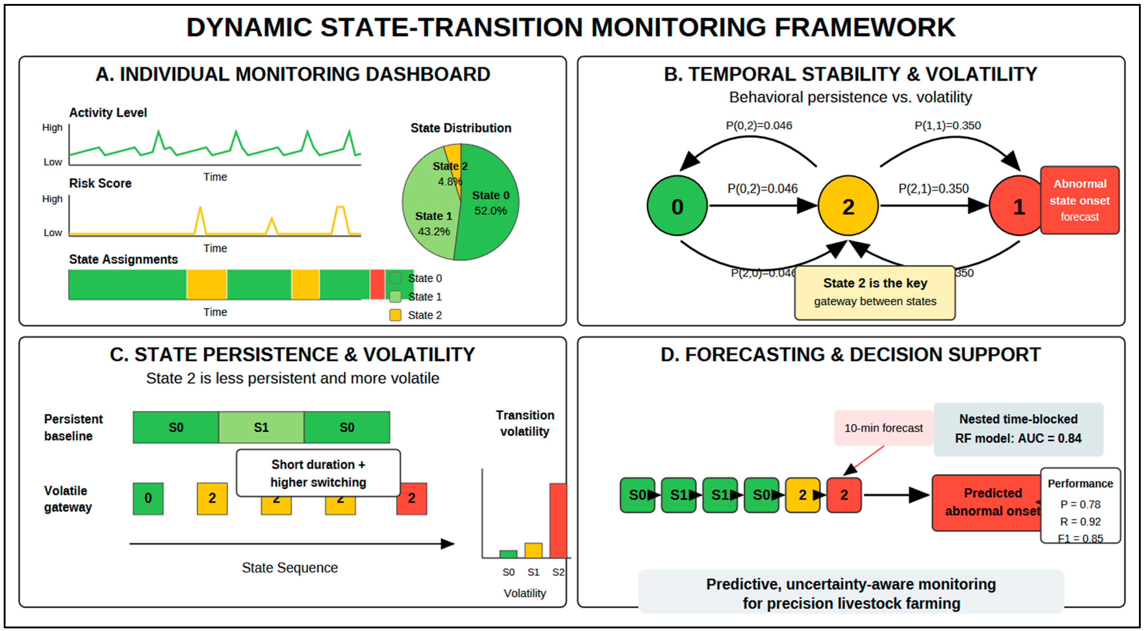
The implemented dashboard provided an interactive prototype animal-level interface for activity visualization, risk scoring, and state monitoring (Figure 7). To summarize how state persistence, transition dynamics, and short-horizon forecasting were operationally linked within this monitoring system, an integrative dynamic state-transition digital twin-oriented framework was constructed (Figure 8).

4. Discussion

This study shows that goat activity data can be modeled as a dynamic behavioral system rather than as a set of isolated activity labels. By combining latent-state discovery, uncertainty analysis, transition modeling, supervised prediction, and dashboard-level deployment, the framework moves beyond conventional behavior recognition toward a more operational form of animal-level monitoring. Importantly, the operational state labels used in the digital twin-oriented framework were not numerically equivalent to the original cluster labels, because the final three-state representation incorporated both latent cluster structure and time-aware behavioral context. The use of nested validation is important in this context because repeated observations from the same goats and short-term temporal dependence can otherwise inflate apparent predictive performance. Accordingly, all preprocessing and model-selection steps were restricted to inner training folds, while outer folds were kept fully untouched for final performance estimation. This is important because most previous goat-monitoring studies have focused mainly on identifying predefined behaviors at single time points, whereas practical livestock AI systems must also determine whether behavior is stable, shifting, or moving toward a higher-risk condition [1,2,5,7,20].

A central finding of this study is that the behavioral stream was dominated by one major low-activity cluster, while the remaining clusters captured smaller but distinct activity regimes. Rather than supporting a simple low-versus-high activity interpretation, the clustering results suggest that goat behavior is organized into multiple behavioral conditions with different temporal patterns [10]. This is important because it indicates that activity data contains more than instantaneous intensity information; they also preserve signals related to behavioral direction, short-term change, and state organization. In that sense, the present framework extends earlier goat behavior work by treating activity as a structured time-dependent process rather than only as a classification target [5,8,9]. This approach is well placed to support and extend advances in animal health monitoring, which also increasingly consider transitions between states rather than classification of current state only [24].

The uncertainty and boundary-region analyses further strengthen this interpretation. A substantial share of observations fell into mixed or low-confidence regions, indicating that behavioral change often occurred through intermediate states rather than through sharply separated boundaries. For livestock AI, this is a useful result because transitional regions may be more informative than fully expressed abnormal states. In applied monitoring systems, those intermediate observations can support graded alerts, risk prioritization, and earlier intervention, which are more practical than binary normal-versus-abnormal decisions. This also distinguishes the present study from many earlier behavior-recognition pipelines, which tend to stop once a class label has been assigned [5,7]. Importantly, the predictive validation analysis showed that boundary-zone and fuzzy-uncertain observations were not only descriptive clustering artifacts, but were also associated with substantially higher odds of future high-activity/non-baseline state onset within 5 min and 10 min forecasting windows.

The temporal stability results also highlight why animal-level analytics are important. Although all goats were dominated by the same baseline cluster, the amount of time spent in non-baseline states varied across individuals. This indicates that herd-level summaries alone would hide meaningful between-animal differences in behavioral activity instability. For precision livestock farming, this is a key point, as the practical goal is often not to describe the average herd, but to identify which animals are deviating from the common pattern and when. The present framework supports that need by preserving individual state occupancy, temporal persistence, and per-animal behavioral profiles, which is consistent with the broader shift toward animal-level decision support in PLF systems [1,2].

The transition analysis provides one of the most useful biological and computational insights in the study. Two states were relatively persistent, whereas one state showed lower stability, higher volatility, and higher entropy, indicating that activity instability in this system was transient rather than sustained. More importantly, the transition pattern suggests that behavioral disruption generally emerged through an intermediate state instead of appearing directly from baseline. This process-based view is important for agricultural AI because it shifts the monitoring problem from detecting a rare endpoint to tracking the pathway leading to it. In other words, the intermediate state becomes the most relevant target for early warning, since it appears to function as the main gateway into activity instability and the main route back toward recovery [13]. Transition through intermediate health states during decline and recovery is also evident from clinical monitoring systems in goats [25] and is likely to be common for many diseases in this and other species even when they are concealed by diagnostic limitations and portrayed only as binary outcomes (infected/uninfected or affected/unaffected).

The higher-order temporal-dependency analysis further suggests that animal activity states may contain longer temporal memory than is captured by a first-order transition matrix alone. The second-order Markov model improved next-state prediction compared with the first-order model, indicating that recent state history may provide additional information about behavioral progression. However, the first-order matrix was retained in the main framework because it is simple, interpretable, and directly useful for summarizing state persistence, volatility, and transition direction. Future studies with longer, externally validated, multi-farm datasets should evaluate hidden Markov models, semi-Markov models, recurrent neural networks, temporal convolutional networks, or transformer-based temporal models to determine whether more complex temporal architectures improve forecasting and biological interpretability.

The supervised learning results show that these short-term dynamics are not only interpretable but also predictable. All models achieved high discrimination, indicating that recent activity level, local change, and temporal memory carried sufficient information to identify unstable states. At the same time, the models differed in their operational error profiles. SVM and BPNN favored sensitivity, whereas Random Forest provided a more balanced tradeoff between detection and false alarms. That distinction is important for deployment. In a farm monitoring context, the best model is not defined only by the highest AUC, but also by the cost structure of the application. A system intended for aggressive early warning may tolerate more false positives, whereas a routine decision-support system may need a better balance between sensitivity and alert burden. This deployment-oriented interpretation aligns with broader work showing that time-aware livestock behavior modeling becomes more informative when temporal context is preserved rather than reduced to static summaries [1,15]. An important distinction emerged between concurrent classification and prospective forecasting. A limitation of the concurrent classification task is that the activity-defined non-baseline target and predictor variables were both derived from the same RFID activity stream. Therefore, the near-perfect concurrent classification results should be interpreted as evidence of internal separability of the algorithm-defined state system rather than independent biological prediction. For this reason, the short-horizon forecasting analysis provides the more meaningful performance estimate, because it tests whether current and recent activity features can anticipate future entry into an activity-defined non-baseline state under time-blocked validation. Even so, these forecasting targets remain activity-derived and should not be interpreted as clinically validated health outcomes. Random Forest achieved an AUC of 0.869 for the 5 min horizon and 0.841 for the 10 min horizon, with average precision values of 0.612 and 0.670, respectively. These forecasting results are therefore more informative for this study’s prospective claims because they show that future activity instability can be anticipated from recent activity history under time-respecting validation, even though performance is lower than for concurrent high-activity/non-baseline state discrimination.

Accordingly, concurrent classification results were moved to the Supplementary Materials and are treated only as evidence that the algorithm-defined states are internally separable. The main predictive claim of this study is based on the nested time-blocked forecasting analysis, which evaluates whether recent activity history can anticipate future high-activity/non-baseline state onset.

Another strength of the present work is the integration of prediction into a digital twin-oriented monitoring framework. Here, the digital twin framework was not treated as a conceptual label alone, but as a continuously updated animal-level representation combining state assignment, temporal trajectory, risk score, and alert output. This makes the workflow more useful than a standalone classification study because it translates behavioral analytics into an interpretable monitoring interface. For precision livestock systems, that kind of integration is important: producers and managers do not act on latent clusters or model outputs directly, but on signals that summarize whether an animal is stable, drifting, or repeatedly entering high-risk periods. This interpretation is consistent with the growing literature describing digital twins as decision-support systems rather than passive mirrors of sensor data [1,18,26].

The study has clear implications for health- and welfare-related monitoring, even though direct physiological or clinical validation were not included here. The transient and intermediate states identified in this work likely correspond to meaningful deviations from normal activity structure, and in production settings such deviations could be associated with discomfort, disturbance, social pressure, environmental challenge, or early disease-related change. Such change could indicate or even precede declining health [27]. This does not mean that the current system should be interpreted as a diagnostic tool. The present study should be interpreted as a behavioral anomaly and activity instability monitoring framework rather than a validated health, welfare, or disease-diagnosis system. Although the RFID-derived states were cross-checked against routine daily animal observations, no synchronized video annotation, physiological measurements, veterinary diagnoses, parasitological data, or clinical welfare scores were available for independent validation. Therefore, the terms “risk,” “alert,” and “abnormal” are used in an activity-pattern sense and should not be interpreted as confirmed indicators of disease or impaired welfare. Future studies should integrate RFID activity data with synchronized behavioral annotation, environmental records, physiological indicators, parasitological measures, and veterinary assessment to determine whether the inferred activity states correspond to biologically meaningful health or welfare outcomes. Rather, its value at this stage is as an early-warning framework that identifies behavioral activity instability before a full abnormal condition is established. That distinction is important, as automated behavioral monitoring is most useful in anticipating health issues to prompt further investigation rather than replace it, allowing for early action to protect individual and herd health and welfare.

Several limitations should also be acknowledged. First, broader generalization across farms, breeds, management conditions, and environmental contexts remains to be tested because the data appear to represent one operational setting. Second, although the dashboard demonstrates deployment potential, practical adoption would require prospective validation, alert-threshold calibration, and assessment of user-facing performance under routine farm conditions.

The dashboard component should also be interpreted cautiously. The current implementation in Google Colab with Gradio was intended only as a prototype visualization layer and not as a production-ready continuous monitoring system. A practical farm-scale system would require local edge computing or cloud-based infrastructure for real-time data ingestion, persistent storage, automated feature calculation, model inference, dashboard hosting, alert delivery, and periodic model recalibration. Therefore, the present work demonstrates the analytical and visualization concept, while future studies should test a scalable deployment architecture under real farm conditions.

Although the dashboard demonstrates a digital twin-oriented monitoring workflow, it should not be interpreted as a fully bi-directional digital twin at this stage. The term digital twin-oriented is therefore used to describe the architecture and monitoring direction of the framework, rather than to claim a complete operational digital twin. The current system functions as an advanced animal-level monitoring and decision-support interface that integrates behavioral state, recent trajectory, risk score, and alert status. However, a complete digital twin would require additional components, including real-time sensor streaming, continuous model updating, feedback from physiological, clinical, parasitological, or environmental measurements, simulation of alternative management actions, and closed-loop intervention logic. For example, a fully operational livestock digital twin could test whether a predicted activity instability event should trigger closer inspection, targeted health evaluation, environmental adjustment, or automated management response. Therefore, the present framework is best described as a digital twin-oriented behavioral monitoring system and a foundation for future closed-loop digital twin development. Future work should therefore integrate activity-derived states with health, welfare, and environmental data and evaluate the framework under external validation settings to determine how robustly these behavioral states transfer across systems. Realistically, however, calibration would never be fully comprehensive, and this work could proceed dynamically, extending the utility of the decision support system and adapting it to new contexts. The framework presented here provides a starting point for field studies in this direction.

Overall, the main contribution of this study is not simply that goat behavior can be classified automatically, but that activity data can be organized into latent states, tracked through time, translated into predictive risk signals, and embedded within an animal-level digital twin-oriented monitoring framework. This gives the work stronger functional relevance for AI in agriculture, where the goal is increasingly to move from descriptive sensing toward continuous, interpretable, and decision-oriented monitoring systems [3,13,28].

5. Conclusions

This study showed that goat activity data can be transformed into a structured, time-aware behavioral monitoring framework that goes beyond conventional behavior classification. The activity stream was resolved into latent behavioral states with interpretable profiles, including baseline, escalating, recovery, and declining high-intensity conditions. Transition analysis further showed that the high-activity/non-baseline state was transient, volatile, and more likely to emerge through an intermediate state than directly from baseline. Under nested time-blocked validation, future high-activity/non-baseline state onset could be forecast over short horizons, with Random Forest achieving an AUC of 0.869 for 5 min forecasting and 0.841 for 10 min forecasting. These results indicate that recent activity history and short-term temporal dynamics contain useful information for prospective activity instability prediction.

The main contribution of this work is its functional integration. Instead of treating clustering, transition analysis, prediction, and deployment as separate components, the proposed framework combines them into a single digital twin-oriented system for animal-level monitoring. This makes the approach directly relevant to precision livestock farming, where the objective is not only to describe behavior, but also to support short-horizon forecasting of activity instability, track recovery patterns, and inform timely management decisions. Because the available dataset contained activity-derived variables but no concurrent clinical, physiological, or parasitological ground-truth measurements, the present framework should be interpreted as a behavior-based activity instability monitoring system rather than a validated disease-diagnosis model. Future research should integrate physiological, health, and environmental measures to validate the biological significance of the identified states and strengthen the framework for health, welfare, and clinical monitoring applications.