A Weed Location Method Based on MCS-YOLOv8 and Adaptive Filtering

Abstract

To address the challenges of large morphological variations of weed targets, background interference in close-range agricultural images, and limited computational resources for visual perception models, this paper proposes a sequential visual perception method for weed recognition and short-range 3D localization in controlled or semi-controlled close-range precision weeding scenarios. The proposed method consists of two main stages: weed detection and 3D localization. In the detection stage, a lightweight MCS-YOLOv8 model is constructed based on YOLOv8n. MobileNetV3 is introduced to reduce the number of parameters and computational complexity, while CBAM and Shape-IoU are adopted to enhance weed-related feature representation and improve bounding-box regression for irregular weed targets. In the localization stage, RAFT-Stereo is used as the initial disparity estimator, and a detection-guided adaptive WLS depth optimization strategy is designed by using the detection bounding boxes and confidence scores. This strategy refines the target-region depth information and supports short-range 3D coordinate estimation. Experimental results show that MCS-YOLOv8 contains 1.6 M parameters and requires 4.3 GFLOPs. Its mAP@0.5 and mAP@0.5:0.95 reached 94.1% and 65.0%, respectively, which were 2.0 and 2.7 percentage points higher than those of the YOLOv8n baseline. Meanwhile, the number of parameters and FLOPs were reduced by approximately 46.7% and 46.9%, respectively. In the 3D localization experiments under controlled conditions, the mean absolute errors in the X, Y, and Z directions were 2.2 mm, 2.6 mm, and 3.2 mm, respectively, with an average 3D Euclidean error of approximately 4.7 mm. Dynamic target experiments further demonstrated that the proposed pipeline could complete indoor dynamic target recognition, 3D coordinate updating, and laser pointing verification under controlled conditions. The results indicate that the proposed method shows effective weed detection and short-range 3D localization performance under controlled agricultural close-range imaging conditions, and can provide a reference for visual perception and end-effector pointing in controlled or semi-controlled close-range precision weeding equipment.

1. Introduction

Weeds compete with crops for light, water, and nutrients, thereby reducing crop yield and quality [1]. Without timely and effective control, weeds can cause considerable yield losses [2,3]. For close-range precision weeding equipment, especially under controlled or semi-controlled operating conditions, visual perception should not only identify weed targets in images, but also provide their spatial positions for subsequent end-effector operation. Therefore, weed recognition and short-range 3D localization are two closely related tasks in close-range precision weeding scenarios.

Early weed recognition methods mainly relied on traditional image processing and manually designed features, such as color, texture, shape descriptors, threshold segmentation, and active shape models [4]. These methods can achieve weed classification under relatively simple imaging conditions, but their performance is often affected by illumination variation, background interference, occlusion, and large morphological differences among weed species. In recent years, deep learning-based object detection methods, including YOLO-series and Faster R-CNN-based models, have been widely applied to agricultural target detection and weed recognition [5,6]. Compared with traditional methods, these models provide stronger feature representation and better detection accuracy [7,8]. However, close-range weed detection still faces several challenges, including irregular target shapes, large scale variation, leaf overlap, soil background interference, and limited computational resources on agricultural mobile platforms [9,10]. As a result, balancing detection accuracy and model complexity remains an important issue for weed perception systems [11,12].

In addition to 2D recognition, close-range precision weeding under controlled or semi-controlled conditions requires target depth and 3D coordinate information to guide the actuator toward the weed position. Binocular stereo vision provides a feasible solution for short-range depth estimation by calculating disparity between left and right images [13,14,15,16,17]. Nevertheless, weed scenes are challenging for stereo matching because weed leaves are often slender, partially occluded, weakly textured, and mixed with soil or crop background. Traditional stereo matching methods are prone to mismatching, local holes, noisy disparity, and blurred boundary details in such regions. Deep learning-based stereo matching methods, such as RAFT-Stereo, can generate more continuous disparity maps by modeling global matching information [18], but their outputs are still general disparity estimations and do not explicitly use semantic information from weed detection. Therefore, a gap remains between object detection and stereo localization: 2D detection provides category and bounding-box information but lacks depth, whereas general stereo estimation provides depth but may be unstable in weed target regions. How to use detection results to guide disparity refinement for weed regions is still a problem that needs further investigation.

To address the above issues, this paper develops a sequential visual perception method for weed recognition and short-range 3D localization under controlled close-range agricultural imaging conditions. The proposed framework is not a jointly optimized end-to-end model, but a two-stage detection-localization pipeline. In the first stage, a lightweight weed detector, named MCS-YOLOv8, is constructed based on YOLOv8n by introducing MobileNetV3, CBAM, and Shape-IoU to reduce model complexity and improve target feature representation and bounding-box regression for irregular weed targets. In the second stage, RAFT-Stereo is used as an initial disparity estimator, and a detection-guided adaptive WLS depth optimization strategy is further designed by using weed bounding boxes and detection confidence scores as semantic priors. The refined target-region depth information is then used for short-range 3D coordinate estimation and laser pointing verification.

The main contributions of this study are summarized as follows:

• A lightweight weed detection model based on YOLOv8n is constructed for close-range weed recognition. MobileNetV3 is introduced to reduce the model scale, while CBAM and Shape-IoU are used to improve weed feature representation and bounding-box regression under complex backgrounds.
• A detection-guided adaptive WLS depth optimization strategy is designed for weed-region depth refinement. Instead of treating RAFT-Stereo as an independent contribution, this study uses it to obtain the initial disparity map, and further exploits detection bounding boxes and confidence scores as soft semantic guidance to improve target-region depth stability.
• A sequential weed detection–depth refinement–3D localization–laser pointing verification pipeline is established and evaluated under controlled close-range experimental conditions. The results provide a reference for visual perception and end-effector pointing in controlled or semi-controlled close-range precision weeding equipment, while further field validation and acceleration are still needed for practical deployment.

2. Materials and Methods

2.1. Overall Architecture of the Proposed Method

The proposed method follows a sequential detection–localization pipeline rather than a jointly optimized end-to-end architecture. The main objective of this framework is to obtain reliable weed categories and short-range 3D coordinates for end-effector pointing in controlled or semi-controlled close-range precision weeding. In this pipeline, weed detection provides target categories, bounding boxes, and confidence scores; stereo matching provides the initial disparity and depth information; and the detection-guided adaptive WLS module further refines the target-region depth for 3D coordinate estimation. Therefore, depth estimation is used as an intermediate representation for 3D localization rather than as an independent final task.

The overall workflow consists of three core components. First, a lightweight YOLOv8n-based weed detector is used to identify weed targets and output bounding boxes with confidence scores. Second, RAFT-Stereo is adopted as the initial stereo matching module to obtain the disparity map from the rectified binocular image pair. Third, the detection results are used as semantic guidance to construct adaptive WLS optimization weights, so that the depth values in weed target regions can be refined before 3D coordinate calculation.

2.2. MCS-YOLOv8 Network Structure

To address the detection difficulties caused by similar color and texture features among weed targets, crops, and soil backgrounds, as well as leaf occlusion and illumination variation in close-range agricultural images, this paper constructed a lightweight YOLOv8n-based weed detection model, named MCS-YOLOv8, with its network structure shown in Figure 1. While maintaining the overall detection framework of YOLOv8n unchanged, this model is improved from three aspects: backbone feature extraction, neck feature fusion, and bounding box regression loss to enhance the detection accuracy and deployment adaptability of the model in close-range agricultural perception scenarios.

In the backbone network, considering that the original backbone of YOLOv8n still has certain computational overhead in edge device deployment, this paper introduces the lightweight design concept of MobileNetV3 to reconstruct the backbone feature extraction module [19]. While ensuring the basic hierarchical feature extraction capability, the number of model parameters and computational complexity are reduced, thereby improving the deployment feasibility of the model on agricultural mobile robot platforms.

In the neck network, this paper retains the original multi-scale feature fusion path of YOLOv8n and introduces the CBAM attention module at the feature fusion nodes after two upsampling and two downsampling operations [20]. Adaptive weighting is performed on the fused feature maps in both channel and spatial dimensions to enhance the model’s ability to represent key features of weed targets and suppress interference caused by complex backgrounds and occlusion noise.

In the bounding box regression part, this paper adopts the Shape-IoU loss function to optimize the bounding box regression process of YOLOv8n [21]. Compared with traditional IoU-based losses that only focus on overlapping regions, Shape-IoU further considers the matching relationship between prediction boxes and ground truth boxes in terms of scale and shape, thereby improving the model’s localization capability for slender, occluded and morphologically irregular weed targets.

The improved model is named MCS-YOLOv8, where M represents the MobileNetV3 lightweight backbone structure, C represents the CBAM attention module, and S represents the Shape-IoU loss function. The meanings of each module in Figure 1 are as follows: CBH denotes the basic module composed of convolution, batch normalization, and H-Swish activation function; DCBH denotes the module composed of depthwise separable convolution, batch normalization, and H-Swish activation function; Bneck denotes the MobileNetV3 inverted residual structure; GAP denotes the global average pooling; Upsample and Downsample denote upsampling and downsampling operations, respectively; Concat denotes feature concatenation operation; CBAM denotes the convolutional block attention module; and SPPF denotes the spatial pyramid pooling-fast module.

2.2.1. MobileNetV3 Lightweight Backbone Network

In YOLOv8n, the backbone network is responsible for extracting multi-level visual features. Although the original C2f-based backbone has good feature representation ability, it still contains a certain amount of standard convolution operations, which may increase the computational burden when the model is deployed on resource-constrained agricultural mobile platforms. For close-range weed detection, the detector needs to maintain basic hierarchical feature extraction capability while reducing the number of parameters and computational complexity. Therefore, this study introduces MobileNetV3 into the backbone network to improve the lightweight design of YOLOv8n.

Specifically, while keeping the overall detection framework, neck structure, and detection head of YOLOv8n unchanged, part of the original backbone feature extraction structure is replaced by lightweight modules based on MobileNetV3. These modules mainly include depthwise separable convolution and inverted residual structures. Compared with directly increasing the depth or width of the YOLOv8n backbone, MobileNetV3 provides a more suitable trade-off between model scale and feature extraction capability for mobile and embedded perception tasks. It was therefore selected as the lightweight backbone candidate in this study.

The role of MobileNetV3 in MCS-YOLOv8 is mainly to reduce redundant convolution computation and improve model compactness. Its depthwise separable convolution decomposes standard convolution into depthwise convolution and pointwise convolution, thereby reducing the parameter number and computational complexity. The inverted residual structure further helps preserve useful feature information during lightweight transformation. Considering that weed targets in close-range images often have irregular shapes, small local structures, and background similarity with crops or soil, the lightweight backbone transformation is designed to reduce model complexity while maintaining the basic feature extraction ability required for weed recognition.

It should be noted that the MobileNetV3 backbone transformation is mainly introduced for model lightweighting and deployment adaptability, rather than being regarded as the primary source of detection accuracy improvement. The subsequent CBAM module and Shape-IoU loss are further used to enhance feature representation and bounding-box regression for irregular weed targets. Therefore, the introduction of MobileNetV3 in this study is a lightweight adaptation of the YOLOv8n backbone, rather than a fundamentally new backbone architecture.

The lightweight backbone transformation based on the MobileNetV3 bottleneck structure is illustrated in Figure 2.

Based on the above structural design, the introduction of the MobileNetV3 lightweight module reduces the number of parameters and computational complexity of the YOLOv8n backbone while maintaining the basic stability of hierarchical feature extraction. This modification improves the compactness and deployment adaptability of the detection model for resource-constrained agricultural perception scenarios. However, MobileNetV3 mainly contributes to model lightweighting, and its role in improving detection accuracy is limited. Therefore, CBAM and Shape-IoU are further introduced in the subsequent sections to enhance weed feature representation and improve bounding-box regression for irregular weed targets.

2.2.2. CBAM Convolutional Attention Mechanism Module

In close-range weed detection, weed targets often show small local structures, irregular leaf shapes, partial occlusion, and visual similarity with crops or soil backgrounds. After multi-scale feature fusion in the YOLOv8n neck network, useful weed-related features may be weakened by background interference and repeated upsampling or downsampling operations. Therefore, CBAM is introduced into the feature fusion stage of MCS-YOLOv8 to strengthen discriminative weed features and suppress irrelevant background responses.

CBAM is used in this study as a lightweight feature enhancement module rather than a new detection architecture. As shown in Figure 3, it consists of a channel attention module (CAM) and a spatial attention module (SAM) connected in series. The channel attention branch emphasizes feature channels that are more relevant to weed recognition, while the spatial attention branch strengthens the response of target regions in the fused feature maps. This design is suitable for weed detection scenes where the target region is small, the boundary is irregular, and the background texture is easily confused with weed leaves.

In terms of network placement, CBAM is embedded at the key multi-scale feature fusion nodes of the neck network after the concatenation of upsampled features and shallow features. This position allows the module to recalibrate fused features from both channel and spatial dimensions, thereby improving the representation of weed target regions before the detection head. By introducing CBAM in this way, the model aims to enhance weed-related feature expression under background interference and leaf occlusion while keeping the additional computational cost relatively limited.

2.2.3. Shape-IoU Loss Function

In the bounding-box regression task, YOLOv8 commonly uses IoU-based loss functions to optimize the overlap and geometric consistency between predicted boxes and ground-truth boxes. However, weed targets in close-range agricultural images often have slender leaves, clustered distribution, prostrate growth patterns, and large shape variations. Under these conditions, the predicted boxes may show insufficient geometric alignment with the actual weed contours, which can further affect the reliability of subsequent detection-guided depth refinement and 3D localization.

To improve the bounding-box regression quality for irregular weed targets, Shape-IoU was adopted in MCS-YOLOv8. Compared with general IoU-based losses that mainly focus on overlapping area and center distance, Shape-IoU introduces shape- and scale-related constraints into the regression process. As shown in Figure 4, the difference between the predicted box and the ground-truth box is not only reflected in their overlap, but also in the width, height, center offset, and shape consistency. This characteristic is important for weed targets with elongated or irregular leaves.

The Shape-IoU loss used in this study can be expressed as:

$${\mathrm{L}}_{Shape-IoU}=1-IoU+\alpha \cdot {distance}^{shape}+\beta \cdot {\mathsf{\Omega }}^{shape}$$

(1)

where IoU denotes the intersection over union between the predicted box and the ground-truth box, d_shape represents the shape-related distance penalty term, Ω_shape denotes the shape ratio penalty term, and α and β are balancing coefficients. In this study, α = 1.0 and β = 0.5 were used according to the experimental settings. The introduction of Shape-IoU is not intended as a new loss-function design, but as a task-oriented regression optimization for weed detection. By considering shape and scale differences, Shape-IoU helps the predicted boxes better fit slender, clustered, and morphologically irregular weed targets. More accurate bounding boxes are also beneficial for the following detection-guided WLS depth refinement, because the detected boxes are used as semantic guidance for target-region depth optimization.

2.3. Binocular Vision Localization Method

To obtain the three-dimensional spatial coordinates of weed targets, binocular vision systems usually realize depth recovery and coordinate solving based on the disparity relationship between the imaging of left and right cameras combined with the triangulation principle. Among them, stereo matching is the key link in binocular vision localization, and its matching accuracy directly affects the subsequent depth calculation and 3D localization results [13]. In agricultural vision, binocular vision is commonly used for fruit detection and spatial localization [14,15]. However, in complex field environments, affected by factors such as soil texture interference, fragmented edges of weed leaves, overlapping between targets and backgrounds, and local weak texture regions, the initial stereo matching results are prone to noise interference and blurred target boundaries, thereby reducing the 3D localization accuracy of weed targets [16,17].

Based on this, this paper first adopts the RAFT-Stereo algorithm to perform stereo matching on the corrected left and right images to obtain relatively robust initial disparity estimation results [18,22]. Then, combined with the binocular camera calibration parameters, the initial disparity map is converted into an initial depth map. On this basis, a detection-guided adaptive WLS depth optimization method is further introduced [23,24]. Using the target bounding boxes and their confidence information output by the front-end weed detection module as semantic priors, a spatially adaptive smoothing parameter map and a data fidelity weight map are constructed to perform differential optimization on the depth map, so as to suppress background noise while preserving the edge structure information of weed targets as much as possible. The optimized depth results are then combined with camera parameters to realize the solution of the three-dimensional coordinates of weed targets. The overall workflow is shown in Figure 5.

Figure 5 illustrates the overall workflow. The arrows indicate the transmission paths of image and feature data, while the orange, blue, and green squares represent the detection module, the stereo matching module, and their internal sub-modules, respectively.

2.3.1. RAFT-Stereo Stereo Matching

To obtain the initial disparity information for subsequent weed depth estimation, this study adopts RAFT-Stereo to perform dense stereo matching on the rectified left and right images. It should be noted that RAFT-Stereo is used here only as an initial disparity estimator rather than an independent methodological contribution of this study. The initial disparity map generated by RAFT-Stereo provides the depth-related input for the subsequent detection-guided adaptive WLS refinement and 3D localization.

As shown in Figure 6, the stereo matching process of RAFT-Stereo mainly includes four parts: feature extraction, correlation modeling, context encoding, and recursive updating. First, feature encoding is performed on the corrected left and right images to extract multi-scale feature representations; subsequently, by calculating the correlation between the left and right features, a multi-resolution correlation pyramid is constructed to describe the matching relationships under different candidate disparities; on this basis, the context encoder further extracts the global semantic information of the left image and initializes the hidden state; finally, the GRU update unit iteratively generates disparity increments according to the current disparity estimation results and correlation query results, performs recursive refinement on the disparity field, and finally outputs the dense disparity map.

Let the corrected left and right image pair be expressed as Equation (2). After passing through the feature extraction network, the feature representations of the left and right images at the k-th layer can be obtained, as shown in Equation (3); furthermore, a multi-resolution correlation volume is constructed according to the correlation between the left and right features, as shown in Equation (4). In the t-th iteration, the GRU update unit generates the disparity increment $△d^t$ according to the current disparity estimation and correlation query results, and performs recursive updating on the disparity field according to Equations (5) and (6).

$$(I_l,I_r)\in R^{H\times W\times 3}$$

(2)

$$F_l^k,F_r^k=F_{\theta }(I_l,I_r)$$

(3)

where $k\in \left\{1,2,\cdot \cdot \cdot ,K\right\}$, K is the number of layers of the feature pyramid, and $F_l^k,F_r^k\in R^{H_k\times W_k\times C_k}$ denote the feature maps of the left and right images at the k-th layer, respectively.

$$C_{i,j,d}^k={\displaystyle \frac{1}{N}}〈F_l^k(i,j),F_r^k(i,j-d)〉$$

(4)

where $d\in \left[0,d_{\max }\right]$ denotes the candidate disparity range; $〈,〉$ denotes the vector inner product; N is the feature dimension normalization factor.

Iterative disparity optimization: The GRU update operator gradually optimizes the disparity field through an iterative manner. Assuming that the disparity estimation at the t-th iteration is d^t and the hidden state is h^t, the entire workflow can be expressed as:

$$△d^t,h^{t+1}=GR{\mathrm{U}}_{\theta }(g(C,d^t),h^t)$$

(5)

$$d^{t+1}=d^t+△d^t$$

(6)

where $g()$ denotes the correlation lookup function, which extracts features corresponding to the current disparity hypothesis from the correlation pyramid; $△d^t$ is the disparity increment of the current iteration; $h^t$ is the hidden state of GRU, which is used to retain historical optimization information.

Through the above process, RAFT-Stereo provides a relatively dense initial disparity map. However, this output is still a general stereo matching result and may contain noise or uncertainty in weed boundary regions, background-mixed regions, and local homogeneous regions. Therefore, the initial disparity map is converted into an initial depth map and further refined by the proposed detection-guided adaptive WLS method to improve the stability of target-region depth estimation and the reliability of subsequent 3D localization.

2.3.2. Detection-Guided Adaptive WLS Depth Optimization

Although RAFT-Stereo can generate relatively stable initial disparity estimation results, the depth map recovered from the initial disparity may still contain fluctuations in weed boundary regions, background-mixed regions inside detection boxes, and local depth discontinuity areas. If the initial depth map is directly used for three-dimensional coordinate calculation, background pixels and edge transition pixels within the detection box may interfere with target depth statistics, thereby causing deviations in the 3D localization results of weeds.

In this study, the term adaptive filtering refers to the detection-guided adjustment of WLS filtering parameters. Specifically, the smoothing strength and data fidelity weight are no longer fixed over the whole image, but are adaptively adjusted according to the weed detection boxes and their confidence scores.

To address this problem, a detection-guided adaptive WLS depth optimization method is introduced in this study. Instead of directly using the initial depth values inside the detection box for target depth statistics, the proposed method first uses the bounding boxes and confidence scores output by the front-end MCS-YOLOv8 detector as soft semantic guidance for global depth optimization. The detection box indicates the possible weed target region, while the confidence score adjusts the reliability weight and smoothing strength during WLS optimization. After the optimized depth map is obtained, the representative depth value of the weed target is extracted from the refined target region for subsequent 3D coordinate calculation. In this way, different constraints are assigned to high-confidence weed regions, low-confidence regions, and background regions, reducing the influence of background pixels and edge transition pixels on target depth estimation. The basic workflow is shown in Figure 7.

Traditional WLS filtering smooths the depth map by minimizing a global energy function:

$$\mathrm{E}(D)={\displaystyle \sum _p\left[\underset{Data Fidelity Term}{\underbrace{(D(p)-D_{init}(p){)}^2}}+\lambda \underset{Smoothness Term}{\underbrace{{\displaystyle \sum _{q\in N(p)}{w}_{pq}{(D(p)-D(q))}^2}}}\right]}$$

(7)

where $p$ denotes the pixel coordinate, $D_{\mathrm{i}\mathrm{n}\mathrm{i}\mathrm{t}}\left(p\right)$ is the initial depth value converted from the RAFT-Stereo disparity result, $D\left(p\right)$ is the optimized depth value, $N\left(p\right)$ denotes the neighborhood of pixel $p$, $w_{pq}$ is the edge-preserving weight constructed according to local image intensity differences, and $\lambda$ is a globally fixed smoothing coefficient. The first term is the data fidelity term, which keeps the optimized depth close to the initial observation, while the second term is the smoothness term, which suppresses local depth fluctuations. In practice, $w_{pq}$ assigns a smaller smoothing weight to neighboring pixels with large intensity differences and a larger smoothing weight to neighboring pixels with similar intensity values, so that depth smoothing can be performed while preserving local edge structures. However, because $\lambda$ is fixed over the whole image, traditional WLS cannot distinguish weed target regions from background regions.

To introduce detection guidance, the fixed smoothing coefficient $\lambda$ is replaced by a spatially adaptive smoothing map $\Lambda \left(p\right)$, and a confidence-related data fidelity weight map $S\left(p\right)$ is added. The improved energy function is formulated as:

$$E(D)={\displaystyle \sum _p\left[S(p){(D(p)-D_{init}(p))}^2+\mathsf{\Lambda }(p){\displaystyle \sum _{q\in N(p)}{w}_{pq}{(D(p)-D(q))}^2}\right]}$$

(8)

For the $k$-th detected weed target, its bounding box is converted into a binary mask $M_k\left(p\right)$, where $M_k\left(p\right)=1$ indicates that pixel $p$ is located inside the $k$-th detection box, and $M_k\left(p\right)=0$ otherwise. The corresponding detection confidence score is denoted as $s_k$, where $s_k\in \left[\mathrm{0,1}\right]$. Based on $M_k\left(p\right)$ and $s_k$, the adaptive smoothing map and data fidelity map are defined as:

$$\mathsf{\Lambda }(p)={\lambda }_{background}-\underset{k}{\max }\left[M_k(p)·f(s_k)\right]({\lambda }_{background}-{\lambda }_{target})$$

(9)

$$S(p)=s_{\min }+(1-s_{\min })\cdot \max \left[M_k(p)\cdot s_k\right]$$

(10)

where ${\lambda }_{\mathrm{b}\mathrm{a}\mathrm{c}\mathrm{k}\mathrm{g}\mathrm{r}\mathrm{o}\mathrm{u}\mathrm{n}\mathrm{d}}$ and ${\lambda }_{\mathrm{t}\mathrm{a}\mathrm{r}\mathrm{g}\mathrm{e}\mathrm{t}}$ are the basic smoothing coefficients for the background region and target region, respectively, and generally satisfy ${\lambda }_{\mathrm{b}\mathrm{a}\mathrm{c}\mathrm{k}\mathrm{g}\mathrm{r}\mathrm{o}\mathrm{u}\mathrm{n}\mathrm{d}}>{\lambda }_{\mathrm{t}\mathrm{a}\mathrm{r}\mathrm{g}\mathrm{e}\mathrm{t}}$. $S_{\mathrm{m}\mathrm{i}\mathrm{n}}$ is the minimum data fidelity weight used to maintain numerical stability. $f\left(s_k\right)$ is a monotonic mapping function of the detection confidence. In this study, $f\left(s_k\right)=s_k$ is used to map the confidence score to the smoothing adjustment strength. For pixels covered by multiple detection boxes, the maximum response ${\mathrm{m}\mathrm{a}\mathrm{x}}_k\left[M_k\left(p\right)s_k\right]$ is used, so that the box with the highest confidence dominates the guidance weight.

Therefore, the proposed WLS filtering process is adaptive in both spatial location and detection confidence. Different pixels are assigned different smoothing and fidelity constraints according to whether they belong to high-confidence weed regions, low-confidence regions, or background regions.

Equations (9) and (10) show how the confidence score is used in the proposed method. When pixel $p$ is located in a high-confidence weed region, ${\mathrm{m}\mathrm{a}\mathrm{x}}_k\left[M_k\left(p\right)s_k\right]$ becomes large. In this case, $\Lambda \left(p\right)$ decreases toward ${\lambda }_{\mathrm{t}\mathrm{a}\mathrm{r}\mathrm{g}\mathrm{e}\mathrm{t}}$, which means that weaker smoothing is applied to preserve the local depth discontinuity and edge structure of weed targets. At the same time, $S\left(p\right)$ increases, so the optimized depth remains closer to the initial depth observation in reliable target regions. When pixel $p$ belongs to the background or a low-confidence region, ${\mathrm{m}\mathrm{a}\mathrm{x}}_k\left[M_k\left(p\right)s_k\right]$ remains small. In this case, $\Lambda \left(p\right)$ stays closer to ${\lambda }_{\mathrm{b}\mathrm{a}\mathrm{c}\mathrm{k}\mathrm{g}\mathrm{r}\mathrm{o}\mathrm{u}\mathrm{n}\mathrm{d}}$, corresponding to stronger smoothing for suppressing depth noise and local fluctuations, while $S\left(p\right)$ remains close to $S_{\mathrm{m}\mathrm{i}\mathrm{n}}$, allowing for more adjustment during global optimization.

The adaptiveness of the proposed WLS optimization is reflected in three aspects. First, the detection boxes determine where target-aware guidance is introduced, so the optimization is spatially adaptive. Second, the detection confidence scores dynamically adjust both the smoothing strength $\Lambda \left(p\right)$ and the data fidelity weight $S\left(p\right)$, so the optimization is confidence-adaptive. Third, the method performs global energy optimization on the entire initial depth map before target depth extraction, rather than directly calculating the target depth from the unoptimized bounding-box region. Therefore, the bounding boxes are used as soft semantic guidance instead of hard depth-statistical regions, which helps reduce mixed-region artifacts caused by soil pixels, crop leaves, or neighboring weeds inside the detection boxes.

After optimization, the refined depth map can suppress background depth noise while preserving the depth structure of high-confidence weed regions. The optimized depth results are then used for subsequent three-dimensional coordinate calculation of weed targets. It should also be noted that the proposed method still depends on the quality of front-end detection. When the detection box is seriously shifted or a false detection occurs, the guidance parameters may introduce local depth optimization bias, which will be further considered in future field validation and robustness improvement.

3. Experiments

3.1. Data Collection

This study constructed a close-range weed image dataset collected at Davidson Orchard Rural Farm in British Columbia, Canada. The dataset contained 760 original images covering six weed categories. The images were acquired in July 2025 using a DJI Mini platform (SZ DJI Technology Co., Ltd., Shenzhen, China) at a low acquisition height of approximately 30–50 cm, with an image resolution of 2720 pixels × 1530 pixels. Therefore, the dataset should be regarded as close-range agricultural imaging data rather than conventional UAV remote-sensing data. All images were saved in JPG format.

To improve scene coverage within the collected dataset, image acquisition included different illumination and weather conditions, including sunny, cloudy, rainy, daytime, and night-with-auxiliary-light conditions. Multiple shooting angles and typical weed distribution scenes, such as single-weed scenes, mixed-growth scenes, and multi-target scenes, were also included. Nighttime images were collected under controlled auxiliary lighting to maintain image quality. It should be noted that the night-with-auxiliary-light samples may still introduce illumination bias compared with natural daytime images.

The original dataset was divided at the image level into training, validation, and test sets at a ratio of 8:1:1. The training set was used for model training and data augmentation, while the validation and test sets were kept unchanged for model selection and final performance evaluation. Some examples of the collected weed images are shown in Figure 8.

To further describe the composition of the collected images,

Table 1. Statistics of scene-attribute frequencies in the original dataset.

Statistical Dimension	Attribute Category	Attribute Frequency
Weather/Light Conditions	Sunny	312
	Overcast	248
	Rainy	196
	Night with Auxiliary Light	194
	Subtotal	950
Weed Distribution Scenarios	Single-Weed Scenario	286
	Multi-Weed Mixed Scenario	402
	Multi-Target Scenario	262
	Subtotal	950

Note: The values denote scene-attribute frequencies rather than the number of unique images. Since one image may contain more than one scene attribute or weed-distribution characteristic, the total attribute frequency is not necessarily equal to the number of original images.

summarizes the scene-attribute distribution of the original dataset. The statistics in Table 1 are used to describe the frequency of weather, illumination, and weed-distribution attributes in the collected samples. These are scene-attribute counts rather than target category labels for model training. Because one image may contain more than one scene attribute or target-distribution characteristic, the subtotal of scene-attribute frequencies should not be interpreted as the number of unique images.

The collected images provide within-site variation in illumination, weather, viewing angle, and weed distribution. However, these variations are still limited to one collection site and one acquisition period. Therefore, the dataset cannot fully replace cross-region, cross-crop, cross-season, or cross-species data diversity. This limitation is considered when interpreting the generalization ability of the proposed method. To avoid confusion between the number of unique images and scene-attribute statistics, the values in Table 1 are reported as attribute frequencies rather than image counts.

3.2. Dataset Annotation and Augmentation

For the weed detection task, the ground truth was defined as manually annotated weed categories and bounding boxes. LabelImg was used as the annotation tool. Each visible weed instance was annotated with its category label and bounding-box coordinates, and the generated annotation files were used for model training, validation, and testing. Scene attributes such as sunny, rainy, night-with-auxiliary-light, single-weed, and mixed-growth scenes were recorded only for dataset distribution analysis and were not used as target detection category labels.

To improve the training sample variability under the collected conditions and reduce the influence of small-sample training, data augmentation was applied only to the training set after the original dataset had been divided into training, validation, and test sets. The augmentation methods included random rotation, horizontal flipping, vertical flipping, scaling, brightness adjustment, and Gaussian noise perturbation. During augmentation, the bounding-box annotations were transformed synchronously with the images to maintain consistency between images and labels. The validation set and test set remained unchanged to avoid evaluation bias.

After augmentation, the augmented training set contained 2400 training samples. The category-level sample counts before and after data augmentation in the training set are summarized in

Table 2. Category-level sample counts before and after data augmentation in the training set.

Weed Category	Before Augmentation	After Augmentation
Roundleaf toothcup	102	404
Carolina geranium	104	410
Shepherd’s purse	81	321
Canada thistle	98	385
Crabgrass	108	428
Barnyard grass	115	452
Total	608	2400

Note: The values denote category-level training samples or annotated weed instances. Data augmentation was applied only to the training set, while the validation and test sets remained unchanged.

.

Figure 9 further visualizes the category-level distribution of annotated weed instances in the augmented training set. This figure reports instance-level counts rather than per-image category counts. Data augmentation increases the diversity of training samples in spatial position, illumination, and local texture, but it does not replace real data diversity from different geographical regions, crop types, growth stages, and weed species. Therefore, the augmented dataset is used to improve training robustness within the collected dataset, while broader field generalization still requires further validation using more diverse datasets.

To examine the contribution of augmentation to model robustness, corresponding data augmentation ablation experiments are reported in the ablation experiment section.

3.3. Experimental Equipment and Environment Configuration

The training, ablation experiments, and desktop offline inference tests of the weed detection model were conducted on a unified computing platform. The hardware configuration included an Intel Core i5-14400F processor (Intel Corp., Santa Clara, CA, USA) with 10 cores and 16 threads, 16 GB DDR4 3200 MHz memory, and an NVIDIA GeForce RTX 4060 GPU (NVIDIA Corp., Santa Clara, CA, USA) with 8 GB VRAMThe operating system was Windows 11, and the software environment included CUDA 12.3, cuDNN 8.9.7, Python 3.10.12, and PyTorch 2.2.0. During model training, the input images were resized to 640 × 640 pixels, the batch size was set to 32, the number of training epochs was 300, the initial learning rate was 0.01, the momentum parameter was 0.92, the weight decay coefficient was 0.0005, and SGD was used as the optimizer. To ensure a fair comparison among different detection models, all comparison models were trained and tested using the same dataset division, input size, and training strategy.

To evaluate the edge-side inference ability of the lightweight detection module, the trained MCS-YOLOv8 and baseline detection models were deployed on an EAT230 embedded AI edge computing controller (Xinyantong Technology Co., Ltd., Shenzhen, China) for inference testing. The device is equipped with an NVIDIA Jetson Orin NX processor and 16 GB LPDDR5 memory. In the edge-side detection test, each model used a batch size of 1 for single-frame inference, and the input image size was fixed at 640 × 640 pixels. To reduce the influence of initial loading and cache fluctuations, 50 warm-up inferences were performed before testing. The average single-frame inference latency, FPS, and memory usage were then recorded on the test images. The latency statistics included image preprocessing, network forward inference, and post-processing, where post-processing mainly included confidence thresholding and non-maximum suppression. It should be noted that this edge-side test was used to evaluate the deployment potential of the lightweight detection module, rather than the real-time performance of the complete stereo-based 3D localization pipeline.

The 3D localization and depth optimization experiments were conducted using an OAK-D-SR binocular camera (Luxonis Inc., Littleton, CO, USA) to collect left and right image pairs of weed targets under close-range imaging conditions. Both the left and right cameras used 1 MP global-shutter color sensors with a maximum resolution of 1280 × 800, and the binocular baseline was 20 mm. According to the device parameters, the effective short-range measurement range is approximately 30 cm to 1 m, and the minimum ranging distance can reach about 20 cm at 800P resolution. Therefore, the localization experiments were conducted within the effective short-range measurement range of the camera to improve the reliability of binocular disparity estimation and 3D coordinate calculation.

In the 3D localization workflow, the left and right images collected by the OAK-D-SR camera were first calibrated and rectified. The rectified binocular images were then input into RAFT-Stereo to obtain the initial disparity map. RAFT-Stereo used pre-trained weights and was not retrained on the self-built weed dataset. In this study, RAFT-Stereo was used only as an initial disparity estimation module. Its lack of domain-specific training may limit the stability of disparity estimation in some weed boundary regions, weak-texture regions, or background-mixed regions. Therefore, the initial disparity map was first converted into an initial depth map according to the camera focal length and binocular baseline, and the detection-guided adaptive WLS method was then applied to optimize the target-region depth map. Finally, the optimized depth values were combined with the camera intrinsic parameters to calculate the three-dimensional coordinates of weed targets. The input resolution of RAFT-Stereo was set to 1280 × 800, and the number of iterations was fixed at 32 for all localization experiments to ensure experimental consistency.

For computational analysis, the detection module and the stereo-based localization workflow were evaluated separately. The desktop computing platform was mainly used for model training, ablation experiments, offline inference, RAFT-Stereo disparity estimation, WLS depth optimization, and 3D coordinate calculation. The EAT230 embedded AI edge computing controller was used only for edge-side inference testing of lightweight detection models. This separation avoids overstating the edge deployment capability of the complete pipeline. The complete stereo-based localization workflow still has higher computational cost due to RAFT-Stereo, and further acceleration is required before real-time field deployment. The experimental equipment is shown in Figure 10.

3.4. Evaluation Metrics

To evaluate the performance of the proposed MCS-YOLOv8 weed detection model and binocular 3D localization method, this paper constructed an evaluation metric system from four aspects: detection accuracy, model lightweight degree, detection-module inference efficiency, and 3D localization accuracy. Detection accuracy is used to measure the recognition ability for different weed categories; model complexity and inference efficiency are used to evaluate the computational cost and deployment potential of the lightweight detection module; and 3D localization error is used to measure the accuracy of binocular vision and adaptive WLS depth optimization for estimating the spatial position of weeds.

For the detection task, the manually annotated weed categories and bounding boxes are used as ground truth. A prediction is regarded as a true positive (TP) when the predicted category is correct and the intersection over union (IoU) between the predicted bounding box and the corresponding ground-truth box reaches the preset threshold. A false positive (FP) refers to an incorrect detection result, including a background region incorrectly detected as a weed target, a predicted box with an incorrect category, a predicted box whose IoU with the ground truth is lower than the threshold, or a repeated detection of the same target. A false negative (FN) refers to a real weed target that is not successfully detected by the model. Precision characterizes the reliability of detected weed targets, while Recall reflects the ability of the model to find real weed targets.

3.4.1. Evaluation Metrics for Weed Detection Performance

This paper adopts precision, recall, average precision (AP), and mean average precision (mAP) as the evaluation metrics for weed detection performance. Precision represents the proportion of correct detections among all predicted weed targets, and recall represents the proportion of ground-truth weed targets correctly detected by the model. Their definitions are as follows:

$$P={\displaystyle \frac{TP}{TP+FP}}$$

(11)

$$R={\displaystyle \frac{TP}{TP+FN}}$$

(12)

In the equations, TP denotes the number of correctly detected weed targets, FP denotes the number of incorrect detections, and FN denotes the number of missed weed targets. Precision mainly reflects whether the predicted weed targets are reliable, while recall mainly represents the model’s ability to detect real weed targets.

AP (average precision) is an indicator mainly used to individually measure the model’s recognition performance for a specific category; while mAP (mean average precision) is a comprehensive quantitative indicator obtained by averaging the AP results of all categories, whose function is to reflect the overall detection ability of the model across the entire dataset. The corresponding definition formulas for both are as follows:

$$mAP={\displaystyle \frac{1}{n}}{\displaystyle {\sum }_{t=1}^n{\displaystyle {\int }_0^{1}P(R)dR}}$$

(13)

$$AP={\displaystyle {\int }_0^{1}P(R)dR}$$

(14)

This paper simultaneously reports mAP@0.5 and mAP@0.5:0.95. Among them, mAP@0.5 denotes the mean average precision when the IoU threshold is 0.5, which mainly reflects the basic detection ability of the model for targets; mAP@0.5:0.95 denotes the average value of mAP under each threshold when the IoU threshold ranges from 0.5 to 0.95 with a step size of 0.05. Its evaluation standard is more stringent and can better reflect the comprehensive performance of the model in terms of the localization accuracy of weed bounding boxes.

3.4.2. Evaluation Metrics for Model Lightweighting and Detection-Module Inference Efficiency

To evaluate the computational efficiency of the proposed lightweight detection model, this paper introduces indicators such as the number of parameters (Params), computational complexity (FLOPs), model file size (Model Size), single-frame inference latency (Latency), frame rate (FPS), and memory usage. The number of parameters reflects the weight scale of the model, FLOPs reflects the computational amount required for a single forward inference, and the model file size reflects the storage requirement. Inference latency and FPS are used to evaluate the inference efficiency of the detection module on different computing platforms. It should be noted that the edge-side inference test mainly evaluates the lightweight detection module rather than the complete stereo-based 3D localization pipeline. The average single-frame inference latency is defined as:

$$T_{avg}={\displaystyle \frac{1}{N}}{\displaystyle \sum _{i=1}^N(t_i^{end}-t_i^{start})}$$

(15)

where N is the number of test images, and the start time and end time of inference for the i-th image are recorded respectively. The corresponding average frame rate is defined as:

$$FPS={\displaystyle \frac{1000}{T_{avg}}}$$

(16)

where the unit of Tavg is ms, so FPS is calculated by 1000/Tavg. Since the complete 3D localization workflow includes not only the weed detection model, but also RAFT-Stereo disparity estimation, adaptive WLS depth optimization, and 3D coordinate solving, the inference speed of the detection model alone should not be interpreted as the real-time performance of the complete visual localization workflow. When the complete workflow is analyzed, the time consumption of each module can be counted separately, including MCS-YOLOv8 detection time, RAFT-Stereo disparity estimation time, adaptive WLS optimization time, 3D coordinate solving time, and the total time consumption of the complete workflow. The average single-frame time consumption of the complete workflow is defined as:

$$T_{total}=T_{\det }+T_{stereo}+T_{wls}+T_{coord}$$

(17)

where the four terms denote the weed detection time consumption, RAFT-Stereo disparity estimation time consumption, adaptive WLS depth optimization time consumption, and 3D coordinate solving time consumption, respectively. The FPS of the complete workflow is also defined as the corresponding complete workflow frame rate:

$$FP{S}_{total}={\displaystyle \frac{1000}{T_{total}}}$$

(18)

Through the above indicators, the inference efficiency of the lightweight detection model itself and the computational cost introduced by RAFT-Stereo and adaptive WLS can be analyzed separately. This distinction avoids confusing the edge-side detection speed with the real-time capability of the complete stereo-based localization workflow. The following experiments report the inference performance of the detection model on the RTX 4060 platform and the EAT230 embedded AI edge computing controller, while the time consumption of the complete localization workflow is discussed separately when applicable.

3.4.3. Evaluation Metrics for 3D Localization Accuracy

To quantitatively evaluate the spatial localization accuracy, this paper takes the reference spatial coordinates of weed targets as the ground truth coordinates and compares them with the three-dimensional coordinates calculated by the binocular localization algorithm. Let the three-dimensional coordinates obtained from the i-th measurement be (x_i, y_i, z_i), and the corresponding reference coordinates be (x_true, y_true, z_true). Then, the absolute errors in the X, Y, and Z directions are respectively defined as:

$$e_x=\left|x_i-x_{true}\right|$$

(19)

$$e_y=\left|y_i-y_{true}\right|$$

(20)

$$e_z=\left|z_i-z_{true}\right|$$

(21)

To further reflect the overall localization deviation in 3D space, this paper defines the 3D spatial Euclidean error as:

$$e_{3d}=\sqrt{{(x_i-x_{true})}^2+(y_i-y_{true}{)}^2+{(z_i-z_{true})}^2}$$

(22)

On this basis, this paper adopts mean absolute error (MAE), root mean square error (RMSE), standard deviation (Std), and max error as the evaluation indicators for localization accuracy. Among them, MAE reflects the average level of localization errors, while RMSE is more sensitive to large errors. Std is used to reflect the fluctuation degree of localization errors; Max Error is used to evaluate the localization deviation in the worst case. Taking the X direction as an example, the specific definitions of each indicator are as follows:

$$MA{E}_x={\displaystyle \frac{1}{N}}{\displaystyle \sum _i^N{e}_x}$$

(23)

$$RMS{E}_x=\sqrt{{\displaystyle \frac{1}{N}}{\displaystyle \sum _{i=1}^N{e}_x^2}}$$

(24)

$$St{d}_x=\sqrt{{\displaystyle \frac{1}{N-1}}{\displaystyle \sum _{i=1}^N{(e_x-MA{E}_x)}^2}}$$

(25)

$$Ma{x}_x=\max (e_x)$$

(26)

where N denotes the number of samples in the localization experiment. The calculation methods of MAE, RMSE, Std, and Max Error for the Y direction, Z direction, and 3D spatial error are the same as those for the X direction. The three indicators of average error, error fluctuation, and maximum error can evaluate the accuracy and stability of the binocular localization method. This paper also retains relative deviation (RD) as an auxiliary evaluation indicator, which is used to describe the deviation ratio of the measured coordinates relative to the real coordinates. Its definition is as follows:

$$R{D}_{xi}={\displaystyle \frac{\left|x_i-x_{true}\right|}{x_{true}+\epsilon }}\times 100\%$$

(27)

$$R{D}_{yi}={\displaystyle \frac{\left|y_i-y_{true}\right|}{y_{true}+\epsilon }}\times 100\%$$

(28)

$$R{D}_{zi}={\displaystyle \frac{\left|z_i-z_{true}\right|}{z_{true}+\epsilon }}\times 100\%$$

(29)

where epsilon is a small positive number used to avoid abnormal amplification of relative deviation when the reference coordinate is close to 0. Since RD is easily affected by the coordinate scale, this paper takes MAE, RMSE, Std, and Max Error as the main localization accuracy evaluation indicators, and RD is only used as an auxiliary analysis indicator.

4. Results and Discussion

4.1. Ablation Experiments of Weed Detection Model

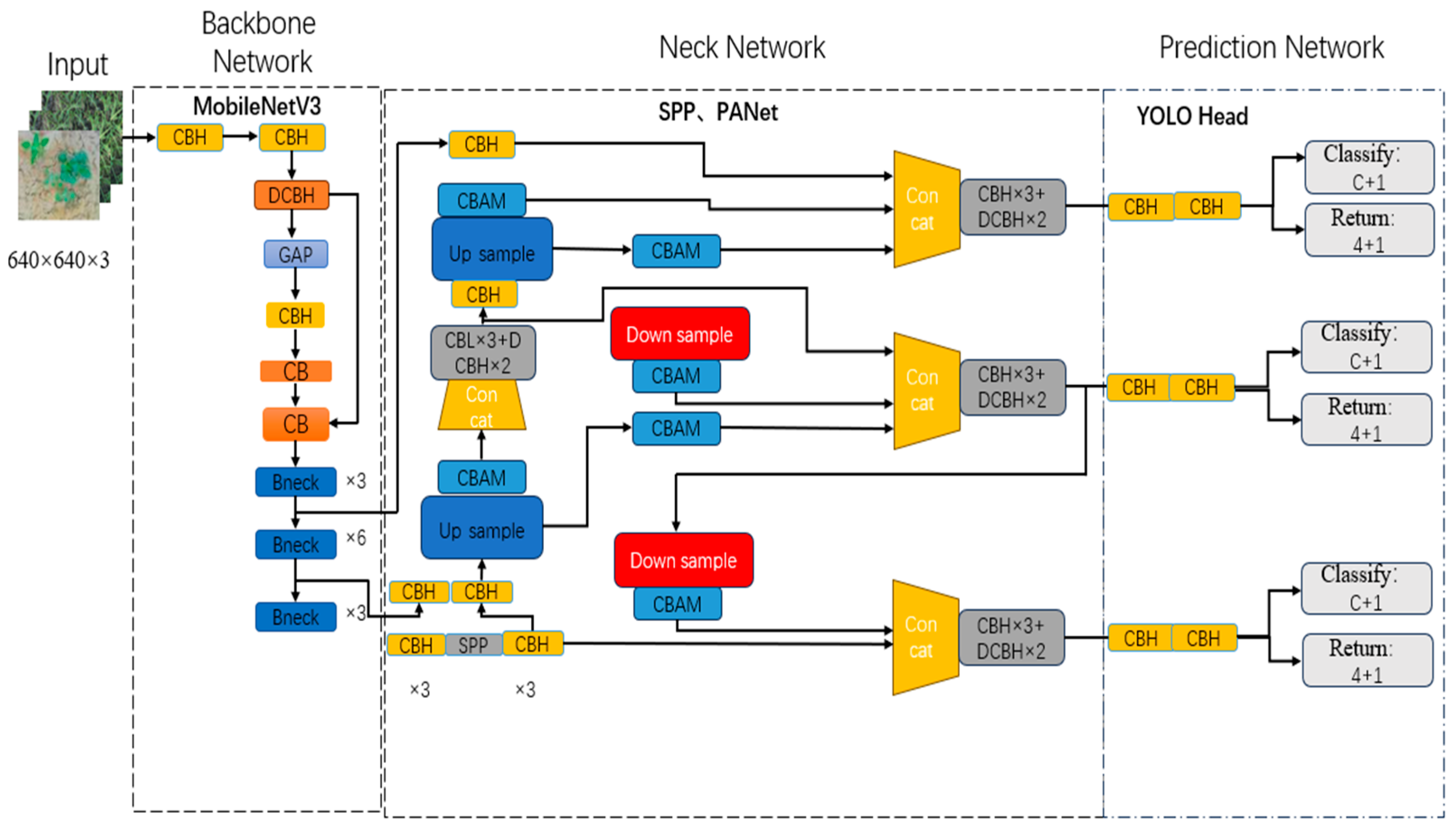
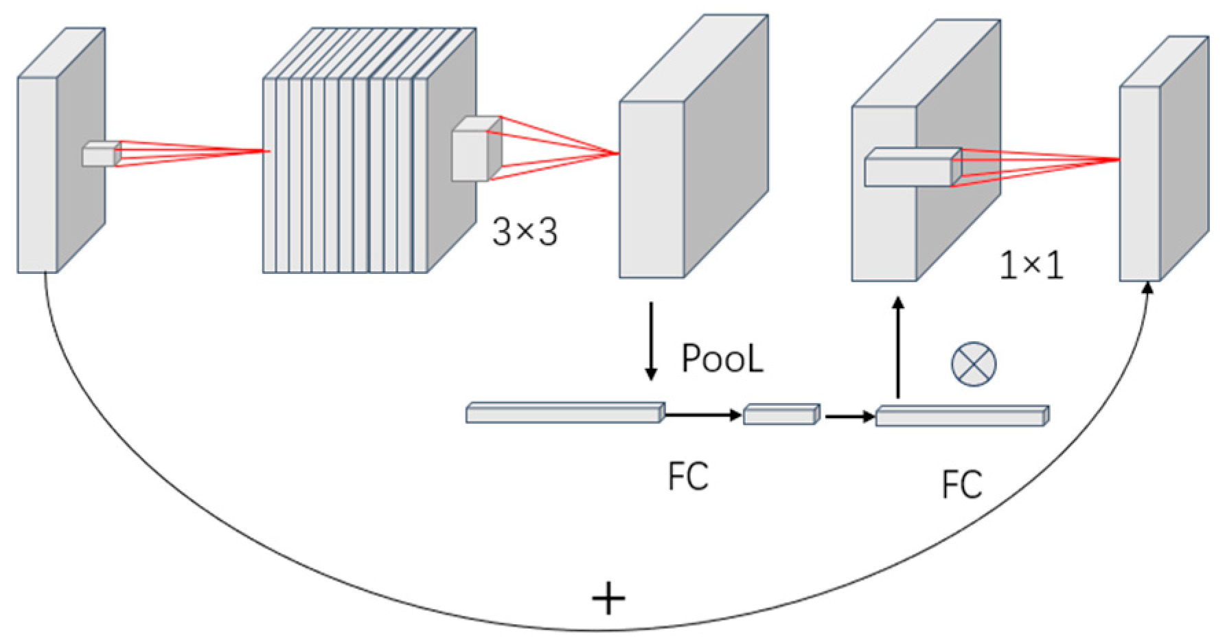
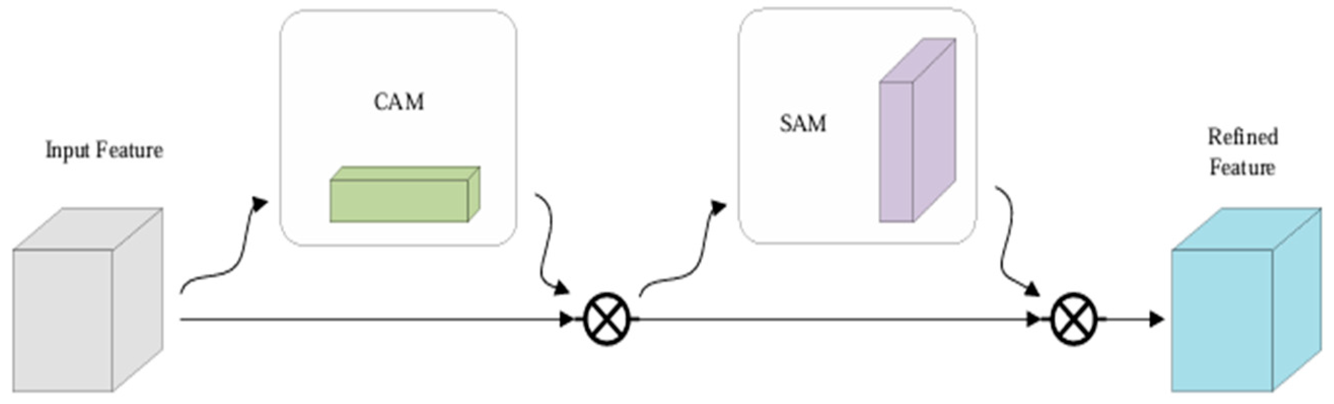
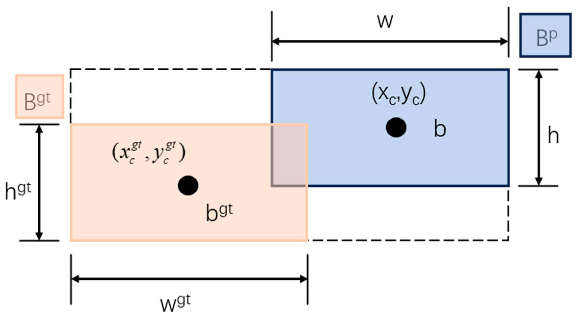
To further verify the effectiveness of each improved module of the proposed weed detection model, this paper conducted ablation experiments on the proposed weed detection model under the same dataset division, input size, and training strategies, to respectively study the impacts of the MobileNetV3 lightweight backbone network, CBAM attention module, and Shape-IoU loss function on the detection accuracy, model complexity, and model compactness of the model. The experimental results are shown in

Table 3. Ablation experimental results of MCS-YOLOv8.

Models	mAP0.5 (%)	mAP0.5:0.95 (%)	FLOPs (G)	Params (M)	Size (MB)	Precision (%)	Recall (%)
YOLOv8n	92.1	62.3	8.1	3.00	6.3	90.4	88.5
+MobileNetV3(M)	92.0	62.0	4.1	1.52	3.3	90.1	88.0
+CBAM (C)	93.0	63.1	8.3	3.08	6.5	91.8	89.2
+Shape-IoU (S)	92.9	63.5	8.1	3.00	6.3	92.2	89.5
M + C	93.3	63.9	4.3	1.60	3.5	91.9	88.8
M + S	93.5	64.2	4.1	1.52	3.3	92.5	89.3
M + C + S	94.1	65.0	4.3	1.60	3.5	93.5	90.2

Note: M denotes MobileNetV3, C denotes CBAM, and S denotes Shape-IoU.

.

It can be seen from Table 3 that introducing MobileNetV3 alone reduced the number of parameters from 3.00 M to 1.52 M and decreased FLOPs from 8.1 G to 4.1 G, corresponding to reductions of 49.3% and 49.4%, respectively. However, the detection accuracy did not improve after using MobileNetV3 alone. The mAP@0.5 slightly decreased from 92.1% to 92.0%, and mAP@0.5:0.95 decreased from 62.3% to 62.0%. Precision and recall also showed slight decreases. This result indicates that MobileNetV3 mainly contributes to reducing model complexity and improving model compactness, rather than directly improving detection accuracy.

After adding CBAM alone to the YOLOv8n baseline, mAP@0.5 and mAP@0.5:0.95 increased to 93.0% and 63.1%, respectively, while precision and recall also increased to 91.8% and 89.2%. This suggests that CBAM helps enhance weed-related feature responses and suppress part of the background interference in close-range agricultural images. After replacing the original bounding-box regression loss with Shape-IoU, mAP@0.5 and mAP@0.5:0.95 increased to 92.9% and 63.5%, respectively, while Params and FLOPs remained unchanged. This indicates that Shape-IoU mainly improves bounding-box regression during training without increasing the inference-stage model complexity.

When MobileNetV3, CBAM, and Shape-IoU were introduced together, MCS-YOLOv8 achieved a mAP@0.5 of 94.1% and mAP@0.5:0.95 of 65.0%, which were 2.0 and 2.7 percentage points higher than those of the YOLOv8n baseline. Meanwhile, the number of parameters decreased from 3.00 M to 1.60 M, and FLOPs decreased from 8.1 G to 4.3 G. These results show that the combined model obtains a better trade-off between detection accuracy and model complexity under the current dataset. It should be noted that the observed improvements were based on the current experimental setting, and the interaction effects among all module combinations still require further analysis in future work.

It can be seen from

Table 4. Detection performance of different bounding box loss functions.

Loss Function	mAP@0.5 (%)	mAP@0.5:0.95 (%)	Precision (%)	Recall (%)	Params (M)	FLOPs (G)
GIoU	93.5	64.0	92.4	89.2	1.60	4.3
DIoU	93.7	64.2	92.7	89.5	1.60	4.3
CIoU	93.8	64.4	93.0	89.7	1.60	4.3
Shape-IoU	94.1	65.0	93.5	90.2	1.60	4.3

that under the premise of unchanged network structure, training parameters, and dataset division, the Params and FLOPs corresponding to each bounding box loss function were basically consistent, indicating that this experiment reduced the influence of model structure changes on the comparison. Compared with GIoU, DIoU and CIoU, Shape-IoU achieved relatively higher results in both mAP@0.5 and mAP@0.5:0.95, as well as precision and recall. Among them, mAP@0.5:0.95 was 0.6 percentage points higher than CIoU, indicating that the bounding box regression of the model for weed targets with irregular shapes was also improved after introducing shape constraints. Although the improvement was not large, Shape-IoU provided a modest but consistent improvement in bounding-box localization accuracy under the current experimental setting.

4.2. Performance Comparison and Edge-Side Inference Analysis of Weed Detection Models

To further verify the comprehensive performance of the proposed MCS-YOLOv8 in weed detection tasks, this paper selected typical object detection models such as Faster R-CNN, SSD, YOLOv5s, YOLOv8n, YOLOv8s, YOLOv8m, YOLOv9-tiny, YOLOv10n, and RT-DETR-L to conduct comparative experiments [25,26,27,28,29]. Among them, YOLOv8n is the baseline model of the improved model in this paper, which was used to evaluate the differences between the proposed MCS-YOLOv8 and traditional detection models, YOLO series lightweight models, and larger-scale detection models [27,28]. This paper adopted training and testing methods under the same dataset division, input size, and training strategies to ensure comparability of the experimental results [29]. For fairness, all detection models were trained and evaluated using the same training, validation, and test split, with the input image size fixed at 640 × 640 pixels. The training epoch number, batch size, optimizer, initial learning rate, momentum, and weight decay were kept consistent with the settings described in Section 3.3. The same data augmentation strategy and evaluation metrics were also used for all models. For models with different architectural characteristics, only model-specific default configuration items that were necessary for normal training were retained, while the dataset split, input resolution, training schedule, and evaluation protocol were kept aligned.

The mAP@0.5, mAP@0.5:0.95, number of parameters, FLOPs, and platform-specific inference frame rates were used as the main evaluation indicators to evaluate the comprehensive performance of different models from three aspects: detection accuracy, model complexity, and inference efficiency. To avoid ambiguity between desktop offline inference and edge-side deployment speed, the FPS results in

Table 5. Performance comparison of traditional, lightweight, and large-scale weed detection models.

Models	mAP0.5 (%)	mAP0.5:0.95 (%)	Params (M)	FLOPs (G)	FPS_RTX (fps)	FPS_EAT (fps)
Faster R-CNN	91.5	60.2	41.5	370.2	18	—
SSD	88.5	57.1	26.3	62.1	48	—
YOLOv5s	92.0	61.8	7.1	15.9	85	—
YOLOv8n	92.1	62.3	3.0	8.1	156	58.1
YOLOv8s	93.0	63.8	11.1	28.4	98	—
YOLOv9-tiny	92.7	63.4	2.0	7.7	145	—
YOLOv10n	93.2	64.0	2.3	6.7	155	—
YOLOv8m	93.2	64.5	25.8	78.7	62	—
RT-DETR-L	94.5	66.0	32.0	110.5	52	—
MCS-YOLOv8	94.1	65.0	1.6	4.3	125	51.0

Note: FPS_RTX denotes the inference speed on the desktop GPU platform equipped with an NVIDIA GeForce RTX 4060, measured in frames per second; FPS_EAT denotes the inference speed on the EAT230 embedded AI edge controller, measured in frames per second. “—“ indicates that the model was not deployed or tested on the EAT230 platform in this study.

are reported separately for the RTX 4060 desktop GPU and the EAT230 embedded AI edge controller.

It should be noted that the compared models in Table 5 are not all lightweight detectors. Faster R-CNN and SSD are included as representative traditional detection models, while YOLOv5s, YOLOv8n, YOLOv9-tiny, and YOLOv10n are used as lightweight or compact detection baselines. YOLOv8s, YOLOv8m, and RT-DETR-L are further included as larger-scale reference models. Therefore, Table 4 is intended to provide a comprehensive comparison among traditional detectors, lightweight YOLO-series models, and larger-scale detectors, rather than comparing only lightweight architectures.

Since the main objective of MCS-YOLOv8 is lightweight weed detection, the comparison with compact models such as YOLOv8n, YOLOv9-tiny, and YOLOv10n is emphasized in the following analysis.

As shown in Table 5, the desktop GPU FPS and edge-device FPS are reported separately. On the RTX 4060 platform, MCS-YOLOv8 achieved 125 FPS, which was lower than YOLOv8n, YOLOv9-tiny, and YOLOv10n, but its mAP@0.5 and mAP@0.5:0.95 were higher than these compact models. On the EAT230 edge device, MCS-YOLOv8 achieved 51.0 FPS, slightly lower than YOLOv8n, but it reduced the number of parameters and FLOPs while maintaining competitive edge-side inference speed.

Compared with larger-scale models such as YOLOv8s, YOLOv8m, and RT-DETR-L, although the detection accuracy of MCS-YOLOv8 was slightly lower, its number of parameters and FLOPs were much smaller, and the inference speed was much faster. For example, the mAP@0.5 and mAP@0.5:0.95 of RT-DETR-L were 94.5% and 66.0% respectively, slightly higher than MCS-YOLOv8, but its number of parameters and FLOPs reached 32.0 M and 110.5 G, which were much higher than the 1.6 M and 4.3 G of MCS-YOLOv8. Overall, MCS-YOLOv8 does not simply pursue the highest detection accuracy, but achieves a better balance between detection accuracy, model complexity, and inference efficiency, which indicates its potential for edge-side weed detection modules in resource-constrained agricultural perception scenarios.

The comparison mainly includes representative general-purpose detectors and recent YOLO/transformer-based object detection models. In addition to these general detection models, related studies have also explored binocular vision-based ranging and localization methods in agricultural or UAV scenarios [30], as well as weed-specific lightweight detection models such as AVGS-YOLO for cotton weed detection in field environments [31]. However, these methods are not directly included in the current comparison because of differences in task objectives, implementation settings, dataset sources, and target categories. In this study, the comparative experiments focused on evaluating the proposed MCS-YOLOv8 under the same dataset division, input size, and training strategy, and cross-dataset evaluation with more weed-specific detection models will be considered in future work.

To further analyze the deployment efficiency of the baseline YOLOv8n and the proposed MCS-YOLOv8, more detailed latency, model size, and memory usage results on the RTX 4060 and EAT230 platforms are reported in

Table 6. Inference efficiency comparison of YOLOv8n and MCS-YOLOv8 on different platforms.

Model	Platform	Params (M)	FLOPs (G)	Size (MB)	Lat (ms)	FPS	Mem (MB)
YOLOv8n	RTX4060	3.00	8.1	6.3	6.41	156.0	620
MCS-YOLOv8	RTX4060	1.60	4.3	3.5	8.00	125.0	540
YOLOv8n	EAT230	3.00	8.1	6.3	17.20	58.1	860
MCS-YOLOv8	EAT230	1.60	4.3	3.5	19.60	51.0	760

Note: Params = parameters; FLOPs = floating-point operations; Size = model size; Lat = average single-frame inference latency; Mem = memory usage.

.

As shown in Table 6, MCS-YOLOv8 had fewer parameters, lower FLOPs, and a smaller model size than YOLOv8n on both test platforms. On the RTX 4060 platform, MCS-YOLOv8 achieved an average inference latency of 8.00 ms and a frame rate of 125.0 FPS. On the EAT230 embedded AI edge computing controller, it achieved an average inference latency of 19.60 ms and a frame rate of 51.0 FPS. Although its FPS was lower than that of YOLOv8n, the proposed model reduced the model size and memory usage while maintaining a relatively high detection-module inference speed. It should be emphasized that these results only evaluate the edge-side inference performance of the weed detection module, rather than the real-time performance of the complete stereo-based 3D localization pipeline.

To further analyze the detection effect of MCS-YOLOv8 on different weed categories, this paper compared the AP values of the YOLOv8n baseline model and the improved MCS-YOLOv8 on each weed category, and the results are shown in

Table 7. AP comparison between YOLOv8n and MCS-YOLOv8 across all categories.

Detect Objects	AP (%) YOLOv8n	AP (%) MCS-YOLOv8
Barnyard grass	84.2	85.8
Crabgrass	89.5	89.1
Canada thistle	76.3	78.1
Shepherd’s purse	82.8	82.5
Carolina geranium	80.1	81.9
Roundleaf toothcup	87.6	88.2

.

It can be seen from Table 7 that the AP of MCS-YOLOv8 improved for most weed categories. Specifically, the AP values of barnyard grass, Canada thistle, and Carolina geranium increased by 1.6, 1.8, and 1.8 percentage points, respectively, indicating that the improved model can enhance the recognition performance for some irregularly shaped weed targets. The AP of roundleaf toothcup also increased by 0.6 percentage points. However, the AP values of crabgrass and shepherd’s purse decreased slightly by 0.4 and 0.3 percentage points, respectively. This may be related to the visual similarity between these weed species, partial occlusion, or differences in sample distribution. Overall, MCS-YOLOv8 improved the overall mAP compared with YOLOv8n, but its category-level improvement was not uniform across all weed species.

Based on the results of Table 6 and Table 7, MCS-YOLOv8 improves the overall detection accuracy while reducing the number of parameters, FLOPs, and model size. However, its FPS was slightly lower than that of YOLOv8n on both platforms. This indicates that lower FLOPs do not necessarily lead to lower inference latency, because actual runtime is also affected by operator type, memory access, hardware acceleration, and deployment optimization. Therefore, MCS-YOLOv8 shows a better accuracy–compactness trade-off for the detection module, but the real-time capability of the complete visual perception pipeline still needs to be analyzed separately, together with RAFT-Stereo, adaptive WLS depth optimization, and 3D coordinate calculation.

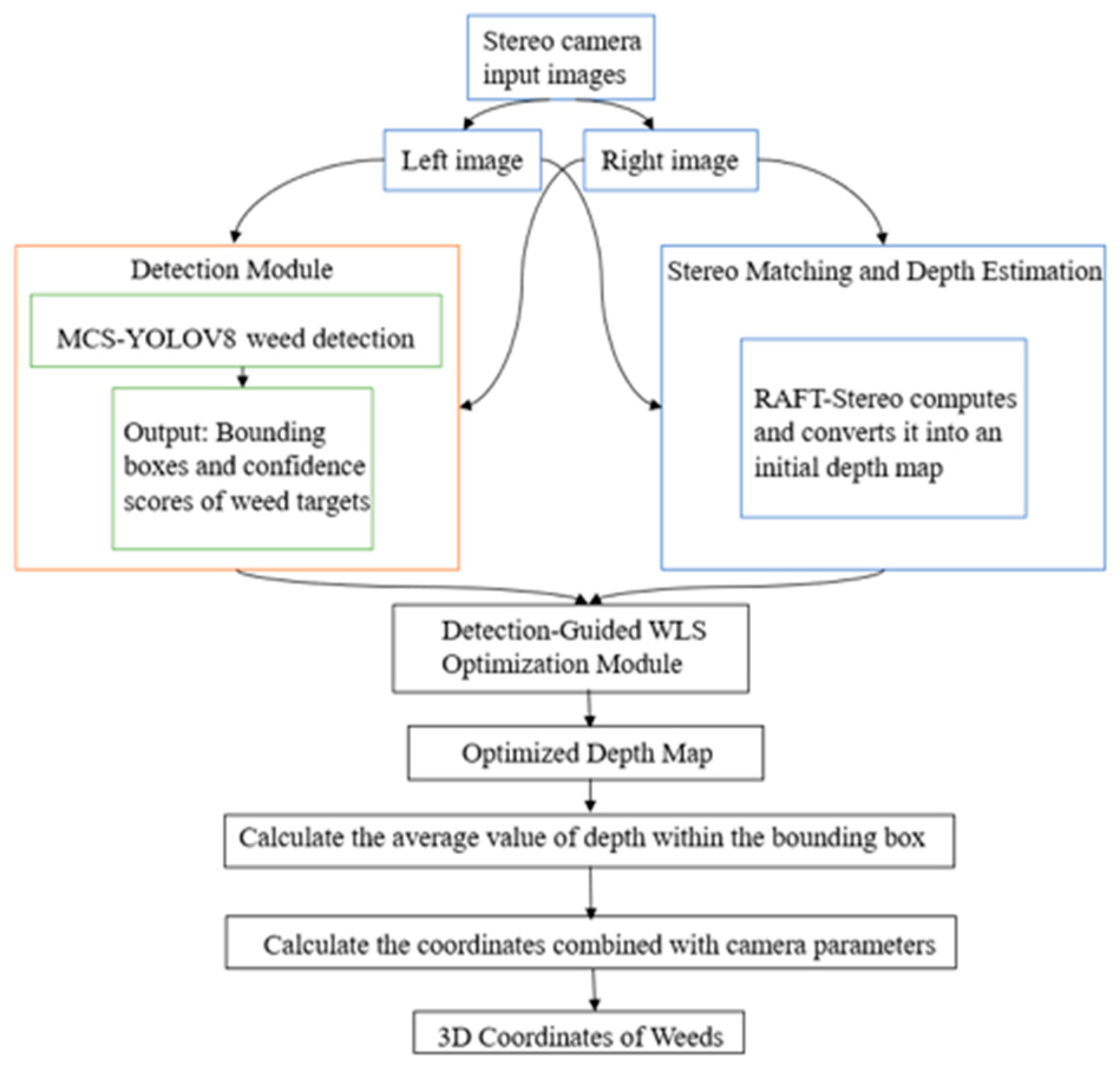
The above experiments mainly evaluated the detection module from three aspects: detection accuracy, model complexity, and edge-side inference efficiency. However, the complete visual perception pipeline proposed in this paper also includes RAFT-Stereo disparity estimation, adaptive WLS depth optimization, and 3D coordinate calculation modules. Therefore, the following sections further analyze the disparity estimation quality, WLS depth optimization effect, 3D localization accuracy, and the computational cost introduced by the complete localization workflow.

4.3. Weed Detection Experiment

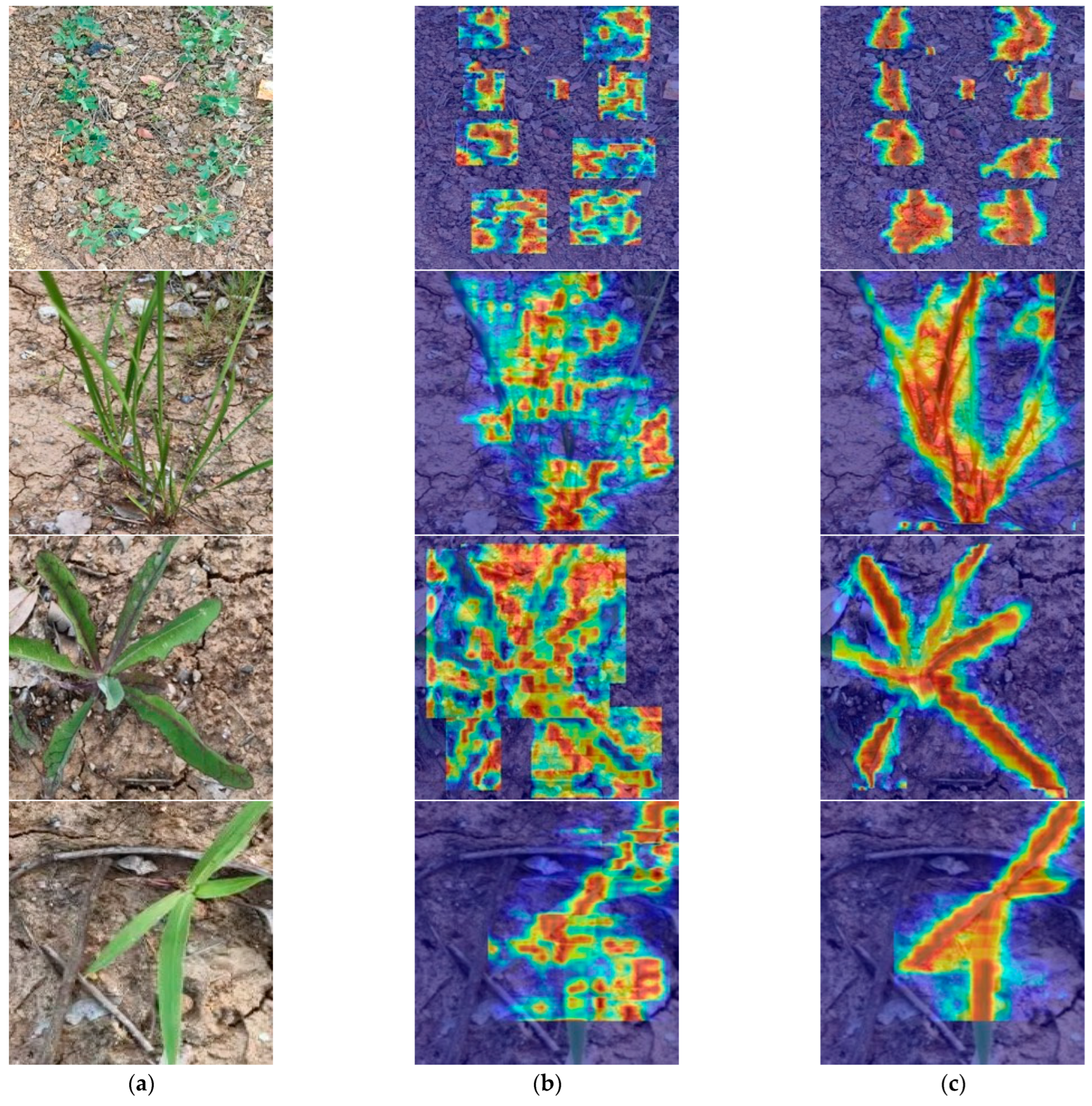
To further analyze the model’s attention to weed target regions, this paper obtained the weed target heatmaps of YOLOv8n and MCS-YOLOv8 at two different scales through KPCA-CAM (Class Activation Mapping method based on Kernel Principal Component Analysis), as shown in Figure 11.

It can be seen from Figure 11 that compared with YOLOv8n, the high-response regions of MCS-YOLOv8 were more concentrated on weed leaves and target body regions, while the responses to background regions such as soil and gravel were relatively reduced. This result indicates that the improved model tends to focus more on weed-related visual features in the displayed samples. To further support the qualitative KPCA-CAM visualization, two attention-distribution indicators were introduced for quantitative analysis. The activation area ratio (AAR) denotes the proportion of high-response pixels in the heatmap, and a lower AAR indicates a more concentrated activation region. The target attention ratio (TAR) denotes the proportion of heatmap response located inside the detected weed target region, and a higher TAR indicates that the model focuses more on weed-related regions rather than background areas.

As shown in

Table 8. Quantitative comparison of KPCA-CAM attention distribution.

Model	AAR ↓	TAR ↑
YOLOv8n	0.386	0.624
MCS-YOLOv8	0.291	0.713

Note: AAR denotes the activation area ratio, where a lower value indicates a more concentrated high-response region (↓: the metric should be minimized). TAR denotes the target attention ratio, where a higher value indicates that more heatmap response is located within the detected weed target region (↑: the metric should be maximized).

, compared with YOLOv8n, MCS-YOLOv8 reduced the AAR from 0.386 to 0.291 and increased the TAR from 0.624 to 0.713. This indicates that the improved model produces a more concentrated attention response and assigns a larger proportion of activation to weed target regions. The quantitative attention-distribution results are consistent with the KPCA-CAM visualization in Figure 11, suggesting that the CBAM attention mechanism and Shape-IoU loss help the model suppress background responses and focus more on weed-related visual features.

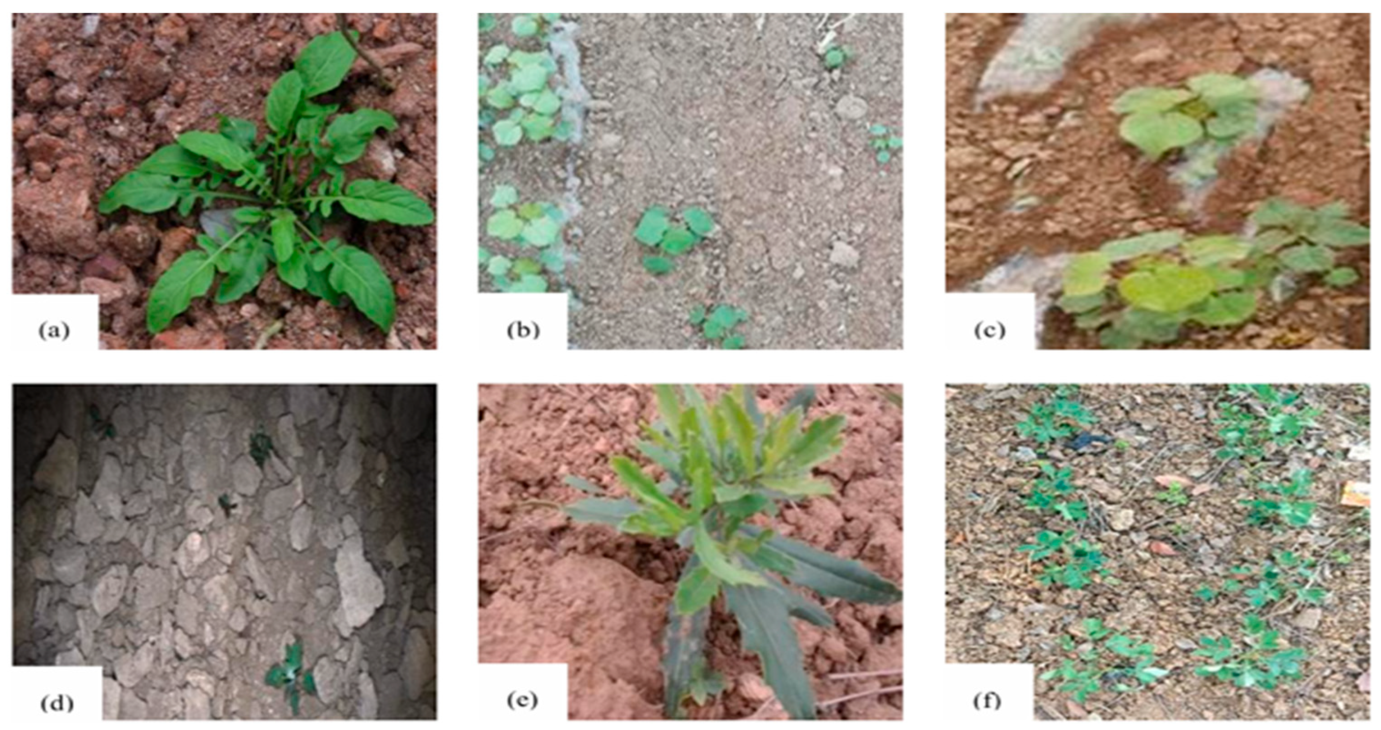
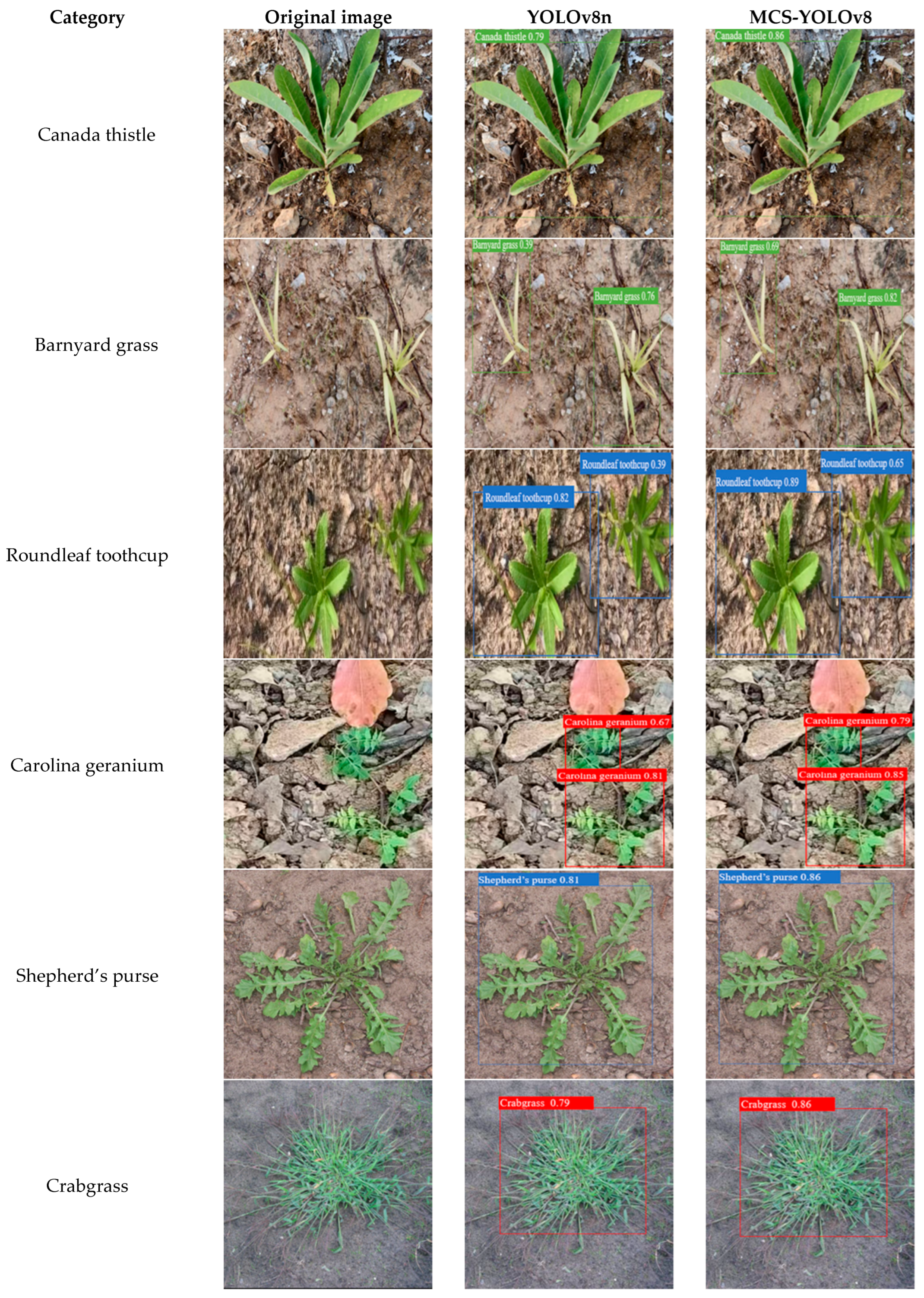
To further provide an intuitive comparison of detection results across different weed categories, representative samples from all six weed categories were selected for visualization. As shown in Figure 12, each row corresponds to one weed category, and the original input image, YOLOv8n detection result, and MCS-YOLOv8 detection result are arranged side by side. This layout allows the performance differences between the baseline and the proposed model to be visually compared under different weed morphologies and background conditions.

The expanded visual comparison shows that MCS-YOLOv8 generally maintains stable bounding-box localization across different weed categories. For categories such as Canada thistle, barnyard grass, roundleaf toothcup, and Carolina geranium, the proposed model shows clearer target localization or higher detection confidence in the displayed samples, which is consistent with the category-level AP improvements reported in Table 6. For shepherd’s purse and crabgrass, the visual differences between YOLOv8n and MCS-YOLOv8 were relatively small, which is also consistent with the small category-level performance gap observed in Table 7. Overall, the expanded visualization provides a more direct category-level comparison between the baseline and the proposed model.

4.4. Localization Experiments and Result Analysis

4.4.1. Comparison of Disparity Estimation Results Between SGBM and RAFT-Stereo

To evaluate the applicability of RAFT-Stereo as the initial disparity estimator in the close-range binocular perception of farmland weeds, this paper selected the traditional SGBM (semi-global block matching) algorithm as a representative comparison method. SGBM is widely used in binocular stereo matching and can reduce local mismatching to a certain extent through multi-directional cost aggregation. However, in close-range weed images, weed leaves are often slender and irregular, while the soil background contains gravel, shadows, and texture noise. Therefore, traditional SGBM may suffer from mismatching, holes, and local noise around weed boundaries and low-texture regions [13].

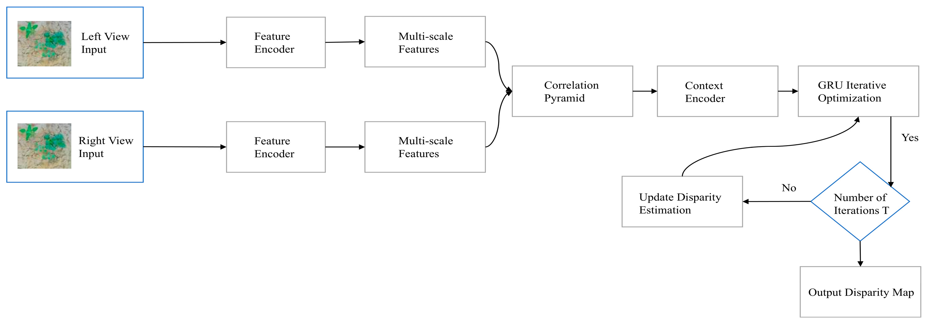
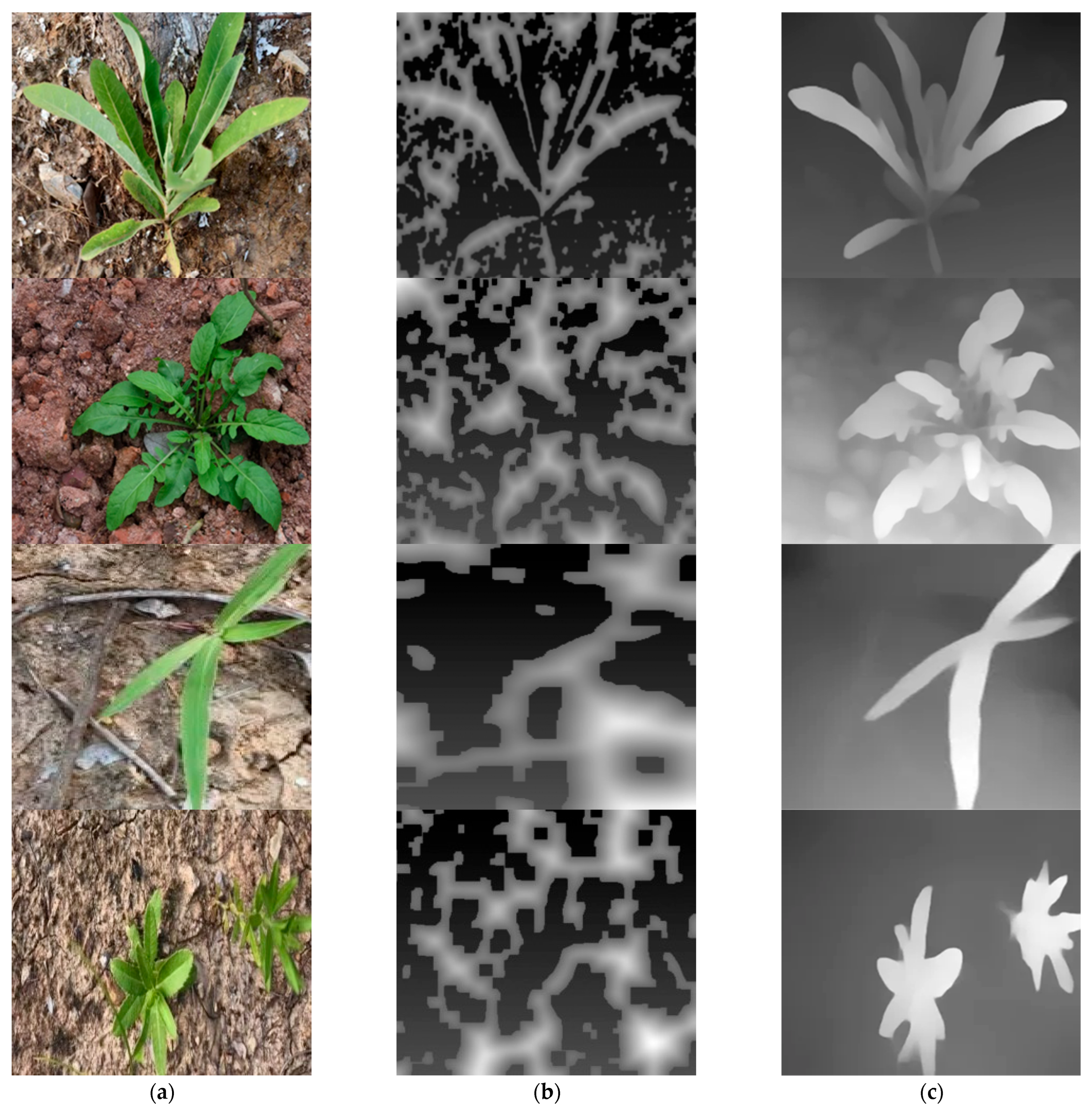
RAFT-Stereo was adopted in this study to obtain the initial dense disparity map for subsequent depth optimization and 3D localization. It should be noted that RAFT-Stereo was used here as an initial disparity estimation module rather than an independent methodological contribution of this paper. Compared with traditional SGBM, RAFT-Stereo can make better use of correlation-volume construction and iterative update mechanisms to produce more continuous disparity results in the displayed close-range weed samples. Since subsequent 3D localization and pointing verification rely on stable target depth estimation, the quality of the initial disparity map directly affects the reliability of the following localization process. Therefore, this paper first provides a qualitative visual comparison between SGBM and RAFT-Stereo, as shown in Figure 13.

It can be seen from Figure 13 that the disparity maps generated by SGBM contain more local noise, holes, and discontinuous regions around the soil background and weed leaf edges. In contrast, the disparity maps generated by RAFT-Stereo are more continuous in the main weed regions, and the leaf structures and target boundaries are clearer in the displayed samples. This visual comparison indicates that RAFT-Stereo can provide a more stable initial disparity map for subsequent depth calculation and 3D coordinate solving.

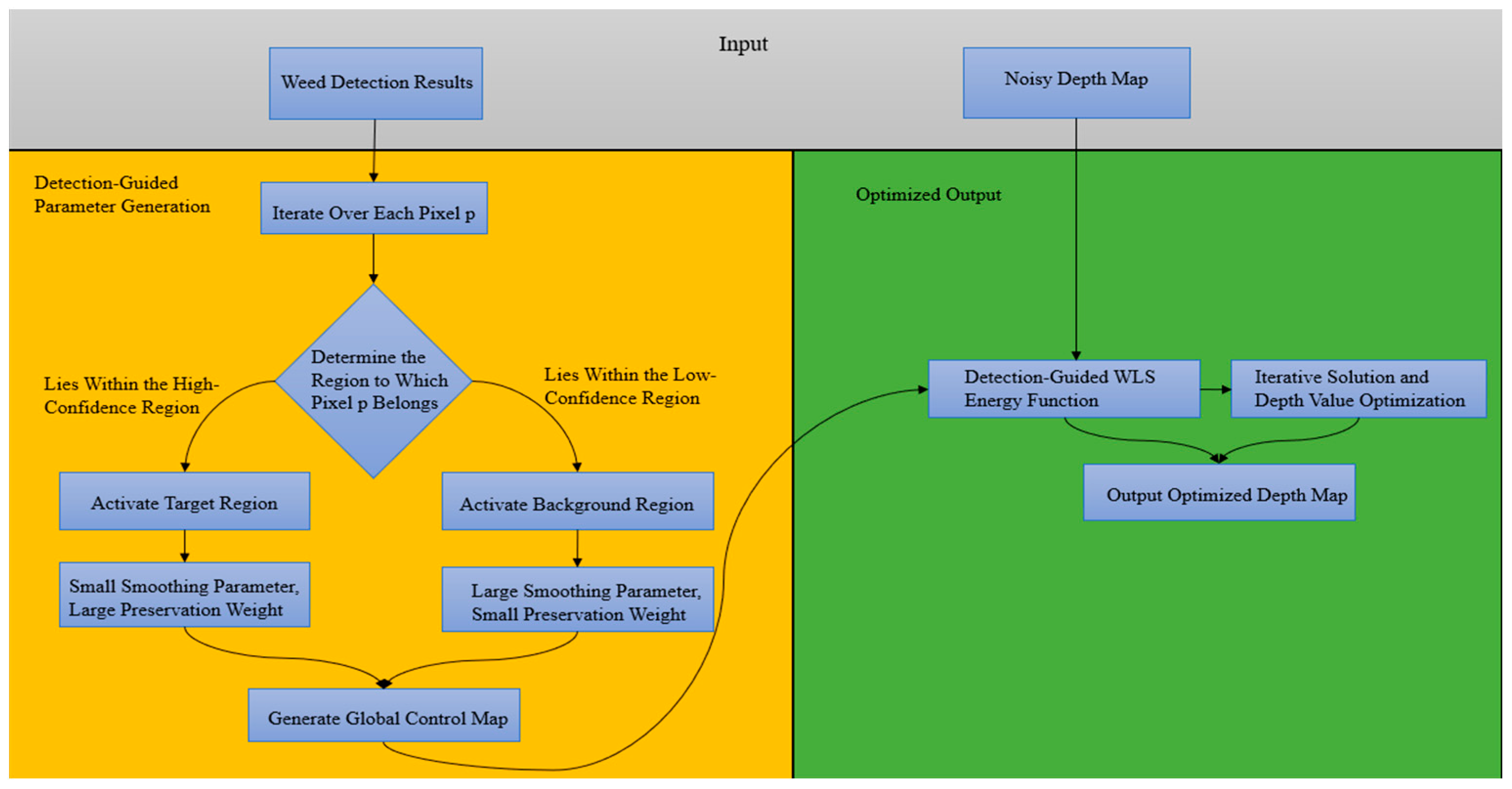
However, this comparison is mainly qualitative and only uses SGBM as a representative traditional stereo matching baseline. It is not intended to serve as a complete benchmark of stereo matching methods. In addition, RAFT-Stereo may still produce disparity blurring or local mismatching around slender leaf edges, target-background junctions, and partially occluded regions. Therefore, based on the initial disparity results provided by RAFT-Stereo, the following section further introduces a detection-guided adaptive WLS depth optimization method to improve the depth stability of target regions and provide a more reliable basis for subsequent 3D localization and pointing verification.

4.4.2. Result Analysis of Detection-Guided Adaptive WLS Depth Optimization

To verify the impact of the detection-guided adaptive WLS depth optimization method on depth measurement accuracy, this paper selected typical weed samples in indoor simulated farmland to conduct close-range depth measurement experiments.

The output result of RAFT-Stereo is not a direct depth map, but a set of disparity maps. Therefore, this paper first takes the output result of RAFT-Stereo as the disparity map for detection-guided adaptive WLS optimization, and then calculates the depth value of the target region according to the camera focal length, binocular baseline, and the optimized disparity value. At three typical close-range measurement positions of 0.3 m, 0.5 m and 0.8 m respectively, 10 groups of binocular images were collected at each distance, and the depth error magnitude of the target region before and after optimization was counted. The experimental results are shown in

Table 9. Depth error statistics before and after adaptive WLS optimization.

TrueDepth (mm)	Method	Avg.Depth (mm)	MAE (mm)	RMSE (mm)	Std (mm)	Max Error (mm)
300	BeforeWLS	312	12	12.6	3.8	18
300	AfterWLS	303	3	3.4	1.6	6
500	BeforeWLS	525	25	26.2	7.8	38
500	AfterWLS	505	5	5.7	2.4	9
800	BeforeWLS	850	50	52.5	15.5	76
800	AfterWLS	808	8	8.9	3.8	14

.

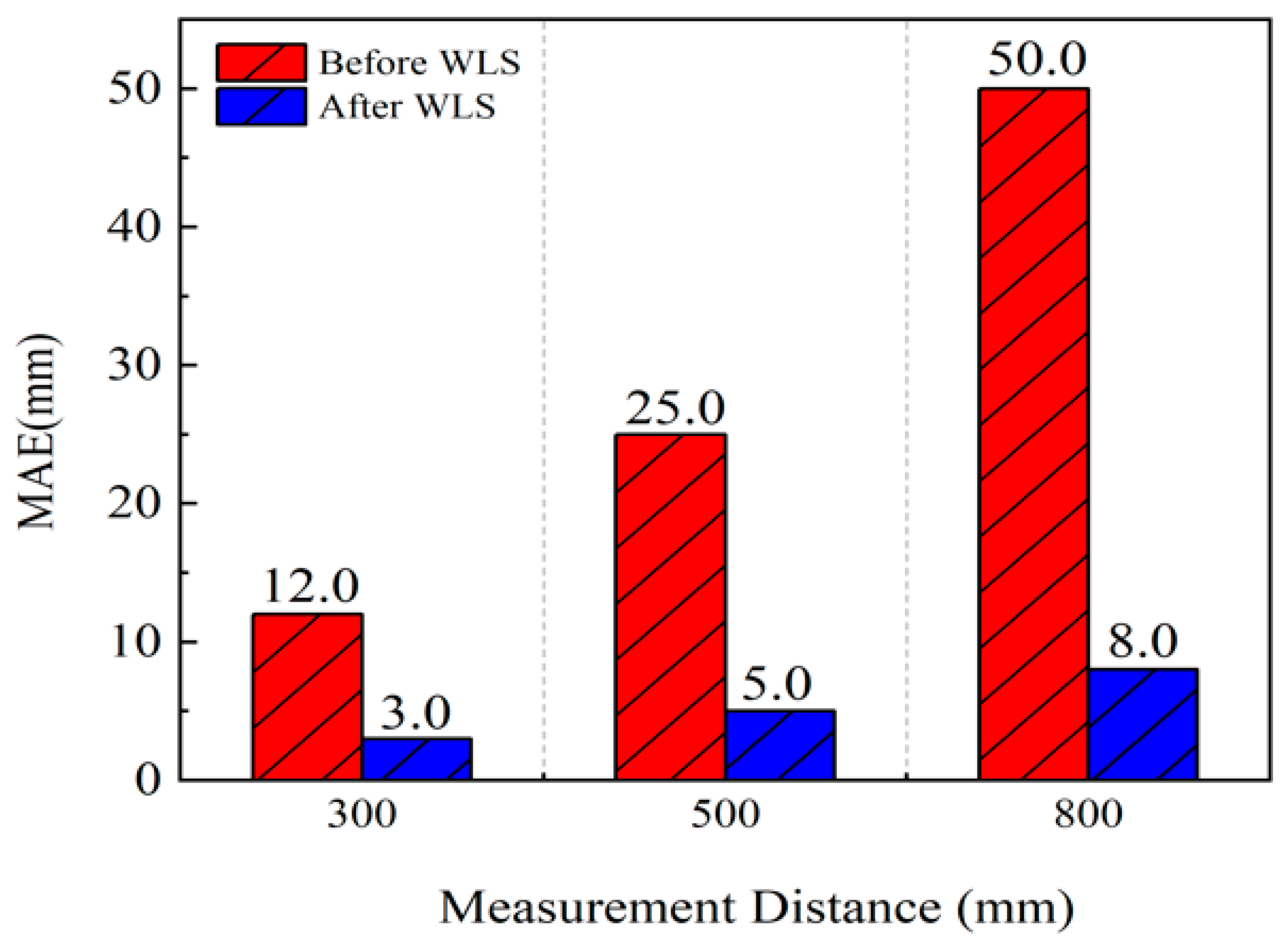
It can be seen from Table 9 that the depth measurement errors at different distances were reduced after detection-guided adaptive WLS optimization. At the measurement distances of 300 mm, 500 mm, and 800 mm, the MAE values decreased from 12.0 mm, 25.0 mm, and 50.0 mm before optimization to 3.0 mm, 5.0 mm, and 8.0 mm after optimization, respectively. The corresponding error reduction rates were 75.0%, 80.0%, and 84.0%. Meanwhile, the RMSE, Std, and Max Error also decreased after optimization, indicating that the proposed WLS refinement can reduce the average depth error, suppress error fluctuation, and improve the worst-case depth measurement performance under the current close-range experimental setting.

To further illustrate the depth refinement effect of the detection-guided adaptive WLS optimization, the MAE values before and after WLS optimization at different measurement distances are visualized in Figure 14.

As shown in Figure 14, the MAE values at 300 mm, 500 mm, and 800 mm were substantially reduced after adaptive WLS optimization. This result is consistent with the quantitative results in Table 7 and indicates that the proposed adaptive filtering strategy can improve target-region depth stability under the current close-range experimental setting.

To further evaluate the runtime performance of the complete 3D localization pipeline, the single-frame processing time of each stage was measured on both the RTX 4060 desktop GPU platform and the EAT230 embedded edge controller. The evaluated stages included weed detection, RAFT-Stereo disparity estimation, detection-guided adaptive WLS depth optimization, and 3D coordinate calculation. The results are summarized in

Table 10. Runtime comparison of the complete 3D localization pipeline on the RTX 4060 and EAT230 platforms.

Platform	Method	Det. (ms)	RAFT (ms)	WLS (ms)	Calc. (ms)	Total (ms)	FPS
RTX 4060	No WLS	8.00	168.40	0	1.12	177.52	5.63
RTX 4060	WLS	8.00	168.40	7.85	1.12	185.37	5.39
EAT230	No WLS	19.60	718.60	0	2.45	740.65	1.35
EAT230	WLS	19.60	718.60	18.40	2.45	759.05	1.32

Note: No WLS denotes the complete 3D localization pipeline without detection-guided adaptive WLS depth optimization, while WLS denotes the complete pipeline with the proposed WLS optimization. Det. = detection inference; RAFT = RAFT-Stereo disparity estimation; WLS = detection-guided adaptive WLS depth optimization; Calc. = 3D coordinate calculation. FPS was calculated from the total single-frame processing time. All tests were conducted with a batch size of 1.

.

As shown in Table 10, RAFT-Stereo disparity estimation was the most time-consuming step in the complete 3D localization pipeline on both platforms. On the RTX 4060 platform, RAFT-Stereo took 168.40 ms per frame, while the MCS-YOLOv8 detection module and 3D coordinate calculation took 8.00 ms and 1.12 ms, respectively. After introducing the detection-guided adaptive WLS depth optimization, the total processing time increased from 177.52 ms to 185.37 ms, and the corresponding FPS decreased from 5.63 to 5.39. The additional latency introduced by WLS was 7.85 ms, accounting for about 4.23% of the total processing time after optimization. This indicates that WLS is not the main computational bottleneck of the complete pipeline on the desktop GPU platform.

On the EAT230 edge controller, the complete pipeline could also be executed, but the processing speed was much lower than that on the RTX 4060 platform. With WLS optimization, the total processing time reached 759.05 ms, corresponding to approximately 1.32 FPS. Among all stages, RAFT-Stereo still dominated the runtime, with an average processing time of 718.60 ms per frame. In contrast, the MCS-YOLOv8 detection module took 19.60 ms on the EAT230 platform, indicating that the lightweight detection module is not the main factor limiting the complete pipeline speed. The WLS module introduced an additional latency of 18.40 ms on EAT230, accounting for about 2.42% of the optimized total processing time.

Combined with the depth error results in Table 10, the detection-guided adaptive WLS optimization improved the depth measurement accuracy of target regions while introducing a relatively small additional computational cost compared with RAFT-Stereo. However, the complete stereo-based localization pipeline only reached about 5.39 FPS on the RTX 4060 platform and about 1.32 FPS on the EAT230 edge controller after WLS optimization. These results indicate that the current complete pipeline has not yet achieved real-time performance for high-speed field deployment, especially on edge platforms. Therefore, the role of WLS in this study should be understood as depth refinement based on the initial RAFT-Stereo output, rather than as an independent depth estimation method or a complete solution for real-time edge deployment. Further lightweight stereo matching, model acceleration, and pipeline optimization are still required before practical real-time field application.

It should also be noted that this experiment was conducted under indoor simulated close-range conditions, and its results mainly reflect the depth refinement effect and runtime characteristics in a controlled setting rather than full outdoor field generalization.

4.4.3. Target and Weed Localization Verification Experiments

After disparity estimation and detection-guided adaptive WLS depth optimization, target localization verification experiments were conducted to evaluate the 3D coordinate calculation ability of the proposed visual perception pipeline. The experimental process is as follows. First, the binocular camera captures the left and right images simultaneously, and MCS-YOLOv8 is used to detect the target region. Then, the rectified binocular images are input into RAFT-Stereo to obtain the initial disparity map, and the target-region depth is refined through detection-guided adaptive WLS optimization. Finally, the 3D coordinates of the target center are calculated in the camera coordinate system according to the camera calibration parameters, and then transformed into the execution-end coordinate system through the hand-eye calibration matrix for laser pointing verification.

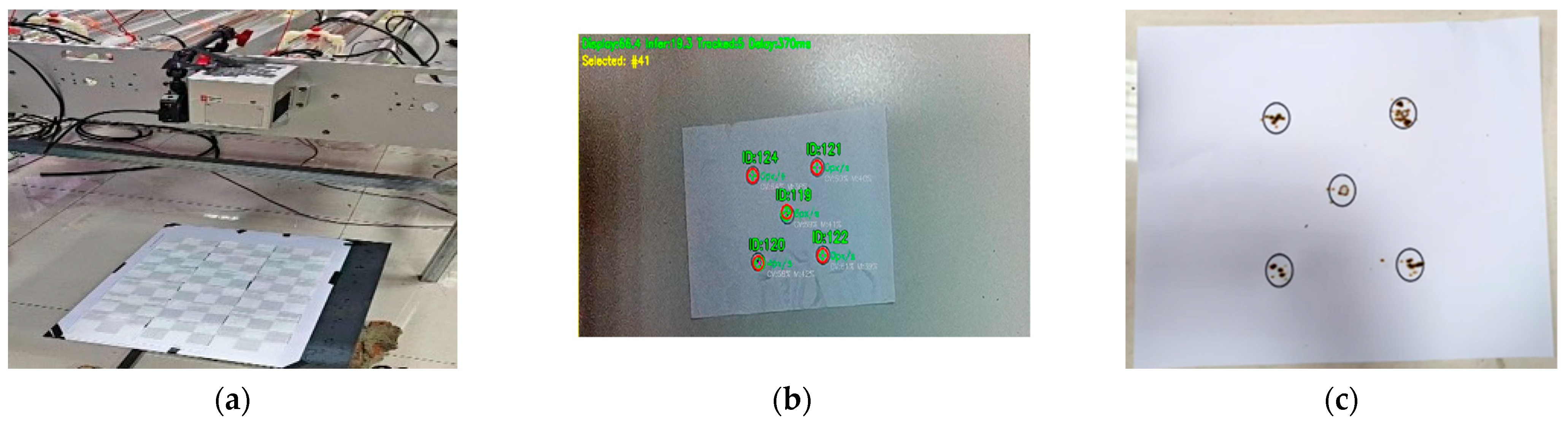
To quantitatively verify the coordinate calculation and coordinate transformation accuracy, five target points with known spatial coordinates were set for static localization experiments. The experimental process is shown in Figure 15, and the target point localization results are shown in

Table 11. Target point localization experimental results.

True Coordinate (mm)	Measured Coordinate (mm)	Coordinate Error (Δx, Δy, Δz)	3D Error (mm)
(150, 150, 492)	(152, 148, 495)	(2, −2, 3)	4.1
(150, 650, 497)	(148, 648, 500)	(−2, −2, 3)	4.1
(400, 400, 503)	(403, 404, 506)	(3, 4, 3)	5.8
(650, 150, 498)	(652, 152, 494)	(2, 2, −4)	4.9
(650, 650, 495)	(648, 653, 498)	(−2, 3, 3)	4.7

.

It can be seen from Table 11 that in the static target localization experiment, the proposed pipeline could estimate the 3D coordinates of the target points with relatively small errors under indoor controlled conditions. According to the localization results, the mean absolute errors in the X, Y, and Z directions were 2.2 mm, 2.6 mm, and 3.2 mm, respectively. The average 3D Euclidean error was about 4.7 mm, and the maximum 3D error was 5.8 mm. These results indicate that the binocular localization pipeline achieved millimeter-level localization accuracy for known static target points in the current indoor experimental setting, providing a basis for subsequent weed target localization and laser pointing verification.

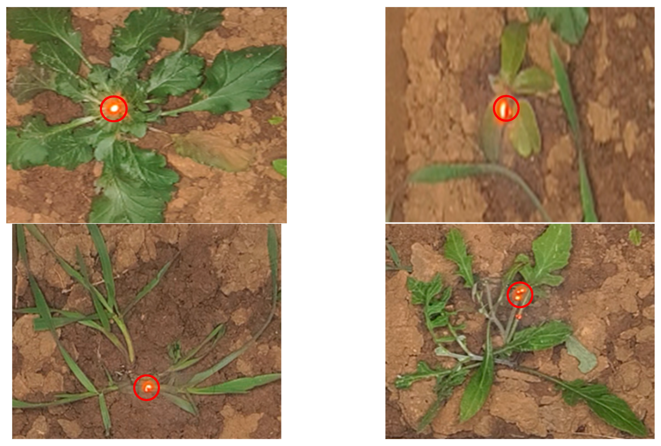
To further provide a visual verification of weed target localization, several representative weed samples were selected as qualitative examples. In these examples, MCS-YOLOv8 first detects the weed target region, RAFT-Stereo and detection-guided adaptive WLS are then used to estimate the target depth, and the target center is finally mapped into the execution-end coordinate system using the hand-eye calibration matrix. As shown in Figure 16, the proposed pipeline can generate target localization points for weed samples with different morphologies and soil backgrounds. However, these weed localization examples are mainly used as qualitative visual evidence. The quantitative localization accuracy is primarily supported by the static target point experiments in Table 11, and further outdoor validation is still required to verify the robustness of the method under more complex field conditions.

4.4.4. Dynamic Target Localization and Laser Pointing Verification Experiments

The aforementioned target and weed localization experiments mainly verified the 3D coordinate calculation ability under static conditions. To further evaluate whether the localization results could support execution-end pointing when the target position changes, dynamic target localization and laser pointing verification experiments were conducted. Different from the static target experiment, the target point in this experiment changes its position by target switching or continuous movement. The system needs to complete image acquisition, target detection, disparity estimation, WLS depth refinement, 3D coordinate calculation, coordinate transformation, and laser pointing response in sequence.

The specific process is as follows. First, the binocular camera synchronously acquires the current target image, and MCS-YOLOv8 detects the target region. Then, the rectified left and right images are input into RAFT-Stereo for initial disparity estimation, and the target-region depth is refined using detection-guided adaptive WLS optimization. The 3D coordinates of the target are calculated according to the optimized disparity, camera focal length, and binocular baseline. Finally, the target position is transformed from the camera coordinate system to the execution-end coordinate system through the hand-eye calibration matrix, and the laser execution end is driven to point to the target center.

In the dynamic pointing experiment, 30 tests were conducted for each dynamic condition. A trial is regarded as successful when the target is correctly detected, the 3D coordinate is updated, and the laser pointing position falls within the preset allowable error range around the target center. Specifically, the pointing error is defined as the planar distance between the laser spot center and the target center on the calibrated target plane. In this study, a trial is considered successful when this distance does not exceed 20 mm. Therefore, the success criterion is based on the distance threshold from the target center rather than simply whether the laser spot falls within the detection bounding box. The target plane is calibrated using a millimeter-scale calibration board, and the image-coordinate distance between the laser spot center and the target center is converted into physical distance in millimeters. Success rate (SR), mean pointing error (MPE), maximum pointing error (MaxE), and average response time (ART) were used to evaluate the dynamic pointing performance. The experimental results are shown in

Table 12. Dynamic target pointing experimental results.

Test Condition	N	Success (%)	Mean Err. (mm)	Max Err (mm)	Resp. (ms)
Target switching	30	96.7	6.8	11.5	185
Target moving	30	93.3	9.4	16.8	236

Note: Success indicates that the target is correctly detected, the 3D coordinate is updated, and the planar distance between the laser spot center and the target center does not exceed 20 mm. MPE and MaxE are calculated based on the laser spot-to-target center distance on the calibrated target plane.

.

It can be seen from Table 12 that under the dynamic target switching condition, 29 out of the 30 tests were successful, corresponding to a success rate of 96.7%. The mean pointing error was 6.8 mm, the maximum pointing error was 11.5 mm, and the average response time was 185 ms. Compared with the static target localization experiment, the pointing error increases because target switching requires the system to update target detection, depth estimation, coordinate transformation, and execution-end pointing after the target position changes.

Under the dynamic target movement condition, 28 out of the 30 tests were successful, corresponding to a success rate of 93.3%. The mean pointing error increased to 9.4 mm, the maximum pointing error reached 16.8 mm, and the average response time increased to 236 ms. This indicates that continuously moving targets introduce higher requirements for visual perception, coordinate update, and execution-end response than target switching. The increase in error and response time is consistent with the higher difficulty of continuous target movement.

The failed or larger-error cases mainly occurred under the dynamic target movement condition. Possible reasons include motion-induced target position changes during image acquisition and processing, local disparity fluctuations around target edges, slight detection-box shifts, and the accumulated delay caused by RAFT-Stereo disparity estimation and execution-end response. In addition, when the target is close to the edge of the field of view or partially occluded by the simulated soil background, the estimated target center and depth may fluctuate, leading to pointing deviation. These results indicate that the proposed pipeline can support indoor dynamic pointing verification, but its robustness still needs to be improved for high-speed field operation and mobile agricultural robot platforms.

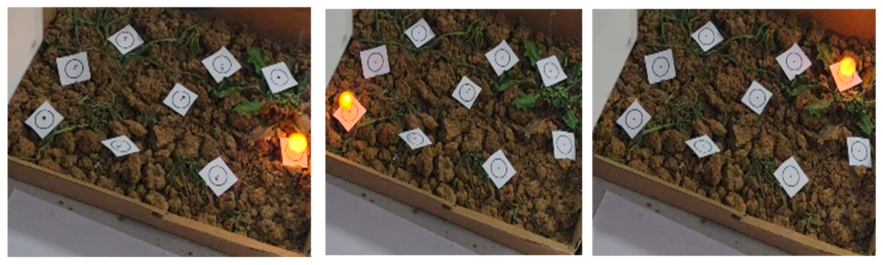
To further intuitively demonstrate the process of dynamic target localization and laser pointing, this paper selected two typical experimental scenarios, dynamic target switching and dynamic target movement, for visual display. The dynamic target switching result is shown in Figure 17. The yellow bright spot in the figure represents the actual pointing position of the laser execution end at the current moment, which is used to reflect the results of the system completing target recognition, 3D coordinate update, and execution end pointing after the target position changes, and to visually assist in explaining the effectiveness of the dynamic experimental results in Table 12.

It can be seen from Figure 17 that during the dynamic target switching process, as the position of the target point changes, the system can re-identify the current target position and drive the laser execution end to point to the corresponding target region. The appearance of yellow bright spots near different target points indicates that the system completes coordinate update and execution end response according to the target switching results. Combined with the quantitative results in Table 12, it can be seen that the proposed method has certain dynamic localization and laser pointing capabilities under indoor dynamic pointing conditions. The visualization results are used as qualitative evidence, while the dynamic pointing performance is mainly supported by the quantitative results in Table 12.

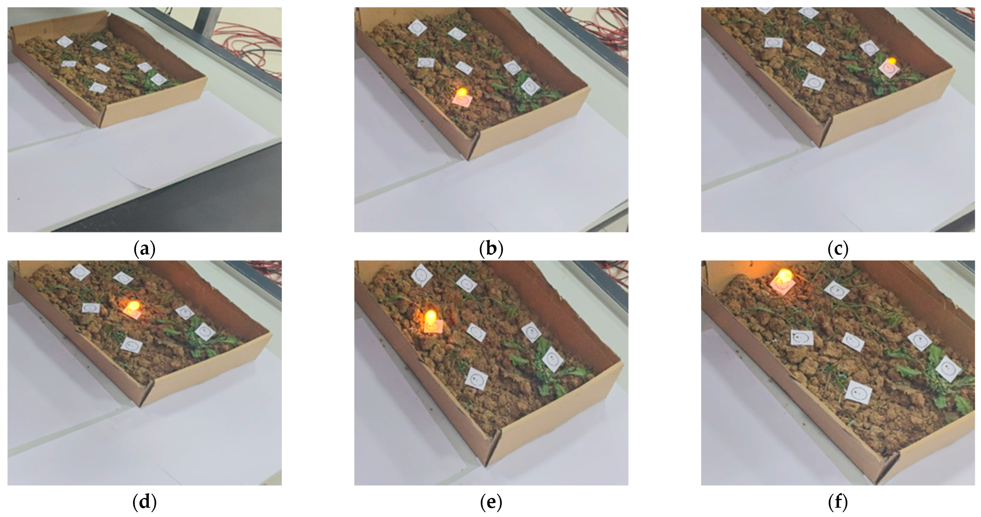
To further simulate the movement of the agricultural robot during operation with the movement of the platform or the movement of the conveying mechanism on its operating area, this paper built a conveyor belt-type dynamic target movement experiment. In this experiment, multiple target points are fixed on the conveyor belt and enter the field of view of the binocular camera sequentially according to the movement of the conveyor belt. The system needs to complete target detection, disparity estimation, 3D coordinate update, hand-eye coordinate transformation and laser execution end pointing under the condition that the position of each target point is constantly changing. Different from the dynamic target switching experiment, this experiment investigates how to locate and point to different target points during continuous conveying.

The experimental process is shown in Figure 18.

It can be seen from Figure 18 that under the condition of conveyor belt-driven dynamic target movement, multiple target points can enter the operating area sequentially with the movement of the conveyor belt. Figure 18a shows the initial movement of the conveyor belt at the beginning of the experiment, and Figure 18b–f sequentially presents the results of the system completing laser pointing on different target points during the movement of the conveyor belt. It can be seen that as the position of the target point changes, the system can timely identify and update the 3D coordinates and point the laser execution end. The yellow laser striking bright spots in the figure all appeared near the corresponding target points, indicating that the system can make continuous responses according to the dynamically changing target positions. Compared with the dynamic target switching experiment, the target position in the conveyor-based dynamic movement experiment changes continuously in the image, which places higher requirements on the response speed of visual perception, coordinate update, and the execution end.

Therefore, it can be seen from Table 12 that the mean pointing error and average response time of the system under dynamic target movement conditions are higher than those under dynamic target switching conditions, which is consistent with the experimental law. From the visual results, although certain dynamic errors occurred during the continuous movement of the target, the system could still complete pointing responses to different target points in the indoor conveyor-based scenario. This indicates that the visual localization pipeline composed of MCS-YOLOv8, RAFT-Stereo, and detection-guided adaptive WLS has a certain dynamic execution capability under controlled indoor conditions.

The experiments in this section mainly verify the feasibility of localization and laser pointing under indoor dynamic target conditions, and they cannot be regarded as equivalent to real field operation on mobile agricultural robot platforms. In practical field operation, platform vibration, natural illumination variation, plant occlusion, irregular terrain, and complex soil background changes may further affect localization and pointing accuracy. Therefore, future work should conduct field dynamic verification on mobile agricultural robot platforms to evaluate the robustness of the complete visual perception and execution pipeline.

5. Conclusions

To meet the requirements of weed recognition, short-range 3D localization, and execution-end pointing verification in controlled precision weeding scenarios, this paper proposed a sequential visual perception pipeline integrating lightweight weed detection, binocular disparity estimation, and detection-guided adaptive WLS depth optimization [32,33]. Considering the irregular morphology of weed targets, soil background interference, and the need for a compact detection model, YOLOv8n was used as the baseline to construct the MCS-YOLOv8 weed detection model. In this model, MobileNetV3 was introduced to reduce the number of parameters and computational complexity, CBAM was used to enhance weed-related feature responses, and Shape-IoU was adopted to improve the bounding-box regression performance for irregular weed targets [34].

For 3D localization, RAFT-Stereo was used as the initial disparity estimation module to obtain a relatively continuous dense disparity map. On this basis, the detection boxes and confidence scores generated by MCS-YOLOv8 were introduced as semantic guidance for adaptive WLS depth optimization. The refined disparity information was then used to calculate the target depth according to the camera focal length and binocular baseline. Finally, the 3D coordinates of the target were obtained in the camera coordinate system and transformed into the execution-end coordinate system through the hand-eye calibration matrix for laser pointing verification [35].

The experimental results show that MCS-YOLOv8 achieved a better trade-off between detection accuracy and model compactness under the current dataset. Compared with the YOLOv8n baseline, mAP@0.5 increased from 92.1% to 94.1%, and mAP@0.5:0.95 increased from 62.3% to 65.0%. Meanwhile, the number of parameters decreased from 3.0 M to 1.6 M, and FLOPs decreased from 8.1 G to 4.3 G, corresponding to reductions of about 46.7% and 46.9%, respectively. Compared with YOLOv9-tiny, YOLOv10n, YOLOv8m, and RT-DETR-L, MCS-YOLOv8 was not the model with the highest FPS or the highest detection accuracy, but it maintained relatively high detection accuracy with a smaller model scale and lower computational cost, showing deployment potential for edge-side weed detection modules.

In the depth measurement experiment, detection-guided adaptive WLS optimization reduced the depth measurement errors at different close-range distances. At the measurement distances of 300 mm, 500 mm, and 800 mm, the depth MAE values decreased from 12.0 mm, 25.0 mm, and 50.0 mm before optimization to 3.0 mm, 5.0 mm, and 8.0 mm after optimization, respectively. The corresponding error reduction rates were 75.0%, 80.0%, and 84.0%. In the static target localization experiment, the mean absolute errors in the X, Y, and Z directions were 2.2 mm, 2.6 mm, and 3.2 mm, respectively. The average 3D Euclidean error was about 4.7 mm, and the maximum 3D error was about 5.8 mm, indicating that the proposed pipeline can achieve millimeter-level localization accuracy for known static target points under indoor controlled conditions [36].

The dynamic target pointing experiments further verified the feasibility of the proposed pipeline under indoor dynamic target conditions. Under the dynamic target switching condition, the success rate reached 96.7%, with a mean pointing error of 6.8 mm, a maximum pointing error of 11.5 mm, and an average response time of 185 ms. Under the conveyor-based dynamic target movement condition, the success rate was 93.3%, with a mean pointing error of 9.4 mm, a maximum pointing error of 16.8 mm, and an average response time of 236 ms. These results indicate that the proposed visual localization pipeline can complete target recognition, 3D coordinate update, and laser pointing response under controlled indoor dynamic conditions. However, larger errors may occur when the target is continuously moving, near the edge of the field of view, or affected by detection-box shift and disparity fluctuation.

Overall, the proposed method provides a feasible visual perception scheme for close-range weed detection, short-range 3D localization, and execution-end pointing verification under controlled or semi-controlled indoor environments. Therefore, the applicability of the proposed method should be interpreted within controlled or semi-controlled close-range indoor scenarios, rather than being directly generalized to open-field precision weeding applications. The current experiments were mainly conducted under indoor or semi-controlled conditions and cannot be regarded as full validation under real field mobile-platform conditions.

In addition, although the MCS-YOLOv8 detection module maintained relatively high inference speed on both the RTX 4060 and EAT230 platforms, the complete stereo-based localization pipeline is still limited by the computational cost of RAFT-Stereo and has not yet achieved high-speed real-time field deployment, especially on edge platforms. In actual farmland environments, platform vibration, natural illumination variation, plant occlusion, irregular terrain, complex soil background changes, and dense weed overlap may further affect detection, disparity estimation, localization, and pointing accuracy. Future work will focus on field dynamic verification using mobile agricultural robot platforms, lightweight stereo matching, edge-side acceleration of the complete pipeline, multi-target continuous tracking, and the integration of visual perception with motion control to improve the robustness and practical applicability of the system.