Development of an Expert Experience Simulator and Hybrid Prediction Model for MPC-Oriented Temperature Regulation in Solar Greenhouses

Abstract

To meet the requirements of precise temperature regulation in solar greenhouses, traditional machine learning algorithms often suffer from poor adaptability, high energy consumption, and difficulties in integrating agronomic expertise. This study developed an intelligent greenhouse temperature regulation framework based on Model Predictive Control (MPC). The core components of the framework include: (1) an expert-experience-based simulator using a Sparrow Search Algorithm-optimized Random Forest (SSA-RF) model to digitize the temperature management strategies of high-yield farmers into dynamic reference trajectories and (2) a hybrid prediction model (CNN-BiLSTM-Attention) combining Complete Ensemble Empirical Mode Decomposition with Adaptive Noise-Permutation Entropy (CEEMDAN-PE) denoising with a Convolutional Neural Network (CNN), Bidirectional Long Short-Term Memory (BiLSTM), and Attention mechanism to achieve high-precision multi-step temperature forecasting. Validation in a cucumber solar greenhouse demonstrated that the SSA-RF model achieved an R² of 0.976 on the test set, showing a significant improvement over the traditional RF model. Compared to the conventional LSTM model, the hybrid prediction model reduced the RMSE to 0.642 and 0.947 for 15 min and 30 min predictions, respectively, with a maximum R² of 0.994 and excellent generalization capabilities. Finally, these two components were theoretically integrated into an MPC-oriented decision framework. The framework describes how expert reference trajectories, multi-step predictions, actuator constraints, and control increments can be combined in a receding-horizon optimization problem. Since online actuator control data were not available, the MPC module was formulated as a theoretical decision framework rather than a fully validated closed-loop controller. This study provides a modelling basis and technical path for future real-time greenhouse temperature control.

1. Introduction

Protected agriculture, as a modern agricultural paradigm, enables high-yield and high-quality production beyond seasonal constraints by constructing controllable crop growth environments [1]. Among various structures, the solar greenhouse is widely adopted in Northern China due to its exceptional energy-saving performance and year-round production capacity, playing a vital role in ensuring vegetable supply [2]. Precise management of the greenhouse microclimate, particularly temperature, is paramount, as it directly regulates core physiological processes such as photosynthesis, respiration, and transpiration, thereby determining crop yield and quality [3].

However, the greenhouse environment is a typically complex system [4], characterized by non-linearity, strong coupling of multiple variables, such as temperature, relative humidity, CO₂ concentration, and vapor pressure deficit (VPD), and high sensitivity to external meteorological disturbances such as solar radiation [5]. This complexity poses significant challenges to maintaining a stable and suitable thermal environment. Traditional control methods rely heavily on grower experience or simple on–off logic, which lack adaptability and precision, often leading to low energy efficiency and suboptimal growing conditions [6].

Previous studies have employed deep learning methods, such as Long Short-Term Memory (LSTM) [7] and Convolutional Neural Networks (CNNs) [8], to predict greenhouse environmental variables. Nevertheless, two major limitations remain when such algorithms are directly applied to control [9]. First, standalone prediction models may lack robustness under extreme or highly variable conditions. Second, purely data-driven models may generate control trajectories that are mathematically optimal but agronomically irrational, as they fail to integrate the valuable management strategies accumulated by experienced growers [10].

To bridge this gap, current research trends are shifting towards the integration of hybrid modelling and optimization algorithms. For instance, signal decomposition techniques such as Complete Ensemble Empirical Mode Decomposition with Adaptive Noise (CEEMDAN) have been utilized to handle noise in non-stationary environmental data [11], while hybrid architectures like CNN-BiLSTM have enhanced the extraction of spatio-temporal features [12,13]. Furthermore, intelligent optimization algorithms, such as the Sparrow Search Algorithm (SSA), have been used to optimize model parameters, improving simulation fidelity [14]. However, a comprehensive theoretical framework capable of systematically integrating high-precision predictors with the digital representation of expert knowledge—and designing explicit control laws for it—remains to be fully explored. Model Predictive Control (MPC) has demonstrated great potential in handling such slow-response, multivariable systems. Its core advantage lies in its ability to linearly handle constraints and optimize control actions within a future time horizon based on dynamic models [15].

Therefore, this study aims to construct a comprehensive theoretical framework for the intelligent temperature regulation of solar greenhouses [16]. The core innovations involve achieving the following objectives stepwise:

(1)

Developing a high-precision multi-step temperature predictor based on a CEEMDAN-PE-CNN-BiLSTM-Attention hybrid model. This model integrates signal decomposition for denoising [17], a CNN for spatial feature extraction [18], BiLSTM for capturing bidirectional temporal dependencies [19], and an Attention mechanism [20] to focus on key time steps.

(2)

Establishing an SSA-optimized Random Forest expert experience simulator. This component digitizes the management patterns of high-yield greenhouses to form ideal temperature reference trajectories reflecting best agronomic practices.

(3)

Formulating an MPC-oriented decision framework by integrating the validated predictor and the expert experience simulator. The framework aims to link expert reference trajectories with multi-step temperature prediction under actuator constraints. It provides a mathematical basis for future closed-loop greenhouse temperature control, which was not formulated as a fully implemented online controller in the present study.

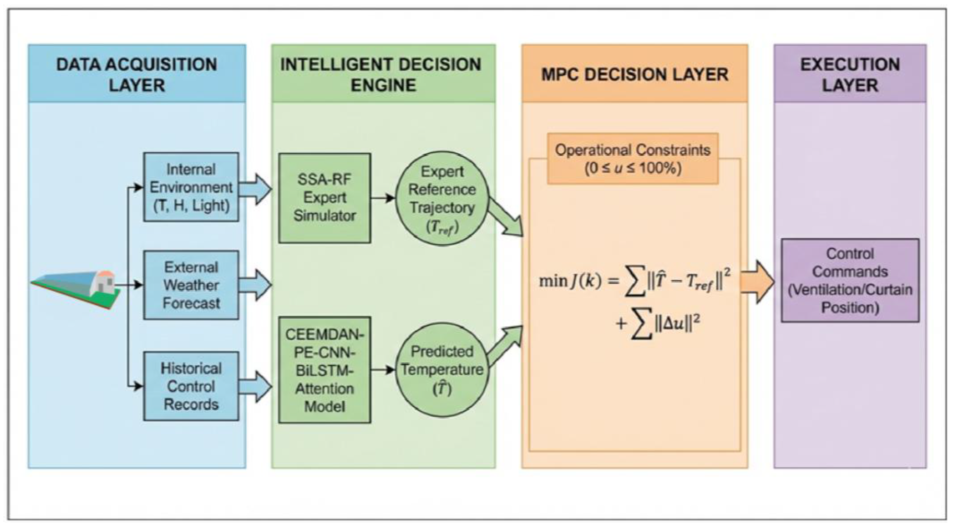
Using experimental data from a cucumber-producing solar greenhouse in Lingyuan, Liaoning Province, China, the two core components—the predictor and the simulator—were fully constructed and validated. Additionally, a receding horizon optimization for the MPC framework was proposed. This framework (Figure 1) not only provides a complete technical path from “perception and prediction” to “decision-making design” for the intelligent upgrading of protected agriculture but also defines the theoretical foundation and core algorithms required for future real-time closed-loop control. It should be noted that this study focuses on the construction and validation of the prediction and expert-reference modules. The MPC part is presented as a theoretical decision-making framework because real-time actuator operation data were not included in the current dataset.

2. Materials and Methods

2.1. Experimental Site and Data Sources

2.1.1. Greenhouse Specifications

Environmental data for cucumber growth were collected from three privately operated, high-yield solar greenhouses located in Siguanyingzi Town (119.58° E, 41.04° N), Dawangzhangzi Town (119.24° E, 41.17° N) and Songzhangzi Town (119.31° E, 41.20° N) in Lingyuan City, Liaoning Province, China. All three greenhouses were of a modern solar design, featuring brick walls reinforced with concrete. The dimensions of the greenhouses were 120 m in length (east–west) and 10 m in width, with a rear wall height of 3.8 m and a ridge height of 5 m. The average annual cucumber yield in these facilities typically reaches 35,000 kg. The common indoor and outdoor environmental variables are presented in

Table 1. Characteristic variables.

Feature Category	Characteristic Variables and Symbolic Representation	Unit
Environmental variables in greenhouse	Air Temperature (Ta)	°C
	Air Humidity (RH)	%
	Soil Temperature (Ts)	°C
	Soil Moisture (RHs)	%
	Carbon Dioxide Concentration (C)	ppm
	Light Intensity (LI)	Lux
Environmental variables outside greenhouse	Daily Mean Temperature (TDa)	°C
	Wind Power/Speed (Wp)	/
	Wind Direction (Wd)	Deg
	Weather Condition (We)	/

.

2.1.2. Data Acquisition System

Outdoor meteorological data, including wind direction, wind speed, weather conditions, and daily average outdoor temperature, were obtained via the Weather API. The indoor environmental data were collected using the MD6A facility intelligent management and control data acquisition system, developed by the Facility Environmental Control Laboratory of Shenyang Agricultural University. The system consists of a device collection terminal and a cloud platform that monitor six categories of indoor environmental data: temperature, humidity, ${\mathrm{CO}}_2$ concentration, light intensity, soil temperature, and soil moisture. The air temperature and humidity sensors were positioned 1.2 m above the ground, while the light intensity and ${\mathrm{CO}}_2$ sensors were placed at a height of 1.5 m. The soil temperature and moisture sensors were installed at a depth of 15 cm in the plant root zone. The data acquisition period spanned from December 2022 to December 2024, yielding a total of 212,637 data points. The sampling frequency was set at 5 min intervals.

2.1.3. Data Analysis and Modelling Environment

The data analysis and model construction in this study were conducted within the PyCharm integrated development environment (IDE) using the Python programming language. Open-source libraries, including NumPy and Pandas, were employed for data processing, while Matplotlib 3.7.2 was used for visualization. The machine learning and neural network architectures were implemented using the Scikit-learn (Sklearn) and Keras libraries, operating on the TensorFlow framework. The specific configuration of the development environment is detailed in

Table 2. The test environment of Python.

Name	Version
CPU	Intel Xeon 4215R
GPU	GeForce RTX4080 16 G
memory	4 × 32 GB DDR4
Operating system	Windows 10 Pro version
Python version	Python 3.9.11
Python library	Sklearn, TensorFlow

.

2.2. Data Preprocessing

Considering the non-linear, strongly coupled, and unstable nature of the greenhouse environment, the raw meteorological data were preprocessed to enhance model training efficiency and prediction accuracy. Outliers were identified and removed using Pau Ta’s criterion (the $3\mathsf{\sigma }$ rule), and missing values were filled via linear interpolation using the Pandas library in Python to ensure data integrity and reliability. Categorical variables, such as wind direction and weather conditions, were numerically recoded to facilitate computational identification. Furthermore, to eliminate the influence of differing scales and numerical ranges among feature variables on the model convergence rate, Min-Max Normalization was applied. This process linearly mapped the data into the [0, 1] interval (

Table 3. Classification table of weather condition variables.

Coded Value	Variable Value	One-Hot Coding
0	Sunny	100
1	Cloudy, cloudy ~cloudy, cloudy ~sunny, fog ~cloudy, cloudy ~cloudy, cloudy, cloudy ~light ~snowy, cloudy ~sunny	010
2	Sleet, cloudy ~ light rain, light rain, light rain ~ cloudy, heavy rain ~ sunny, light rain ~ cloudy, light rain ~ thunderstorm	001

), completing the data normalization. The transformation process is expressed by Equation (1):

$$x_{norm} = {\displaystyle \frac{x - X_{min}}{X_{max} - X_{min}}}$$

(1)

where ${\mathrm{X}}_{\max } \mathrm{and} {\mathrm{X}}_{\min }$ are the maximum and minimum values of the eigenvariable. $x$ is the data in the current sample set. ${\mathrm{x}}_{\mathrm{norm}}$ is the value normalized by x.

The model was built according to the time series, and all data were divided into training sets and test sets according to an 8:2 ratio.

2.3. Feature Selection

To avoid redundancy in the feature selection process, Pearson correlation analysis and RF feature importance ranking were assigned different roles in this study. Pearson correlation analysis was used only as a preliminary and auxiliary method to examine the linear association between each environmental variable and greenhouse air temperature. In contrast, RF feature importance ranking was used as the primary criterion for final input variable selection because it can capture non-linear relationships and interactions among variables. In addition, considering the thermal inertia of solar greenhouses, the selected variables were further organized into temporal input windows to incorporate possible time-lag effects.

2.3.1. Pearson Correlation Analysis

The Pearson correlation coefficient $r$ ranges from −1 to 1. $r > 0$ indicates a positive correlation between two variables, while $r < 0$ signifies a negative correlation. The strength of the correlation increases with the absolute value of $r$. The mathematical expression is given by Equation (2):

$$r = {\displaystyle \frac{{{\displaystyle \sum }}_{i=1}^n\left(x_i - \overline{x}\right)\left(y_i -\overline{y}\right)}{\sqrt{{{\displaystyle \sum }}_{i=1}^n{\left(x_i - \overline{x}\right)}^2}\sqrt{{{\displaystyle \sum }}_{i=1}^n{\left(y_i - \overline{y}\right)}^2}}}$$

(2)

where $\overline{x}$ and $\overline{y}$ represent the mean values of the variables x and y, respectively. The interpretation of the correlation coefficient ranges is summarized in

Table 4. Relationship between the correlation coefficient and correlation.

Correlation Coefficient	Degree of Correlation
$0 \le \left|\mathrm{r}\right| < 0.2$	Extremely weak correlation
$0.2 \le \left|\mathrm{r}\right| < 0.4$	Weak correlation
$0.4 \le \left|\mathrm{r}\right| < 0.6$	Moderately correlated
$0.6 \le \left|\mathrm{r}\right| < 0.8$	Strongly correlated
$0.8 \le \left|\mathrm{r}\right| \le 1$	Extremely strongly correlated

.

In this study, Pearson correlation analysis was not used as the sole basis for feature selection. Its purpose was to provide an intuitive preliminary screening of variables with obvious linear relationships with greenhouse air temperature. The final selection of input variables was determined mainly based on RF feature importance ranking, which is more suitable for describing the non-linear and coupled characteristics of greenhouse microclimate systems.

2.3.2. RF Feature Importance Ranking

Feature selection [21] is critical for enhancing the efficiency of data-driven models. In this study, a Random Forest (RF) model was constructed to calculate and rank the importance of various features. The specific implementation steps were as follows: First, n samples were randomly drawn from the original dataset using the bootstrap method with replacement to construct the training set. Second, decision trees were generated based on these sampled sets; during the construction of each node, d features were selected randomly without replacement, and the optimal splitting feature was chosen based on specific criteria to execute node division. Subsequently, this process was repeated k times to generate a Random Forest comprising k decision trees. Finally, the trained RF was used to predict test samples, with the final prediction determined through majority voting (for classification) or averaging (for regression). This approach enabled the evaluation of the influence weights of different environmental features on greenhouse temperature.

Therefore, RF feature importance ranking was adopted as the main feature selection method in this study, while the Pearson correlation results were used as auxiliary evidence to verify whether the selected variables had reasonable physical and statistical relevance to greenhouse air temperature.

2.3.3. Lag Effect Consideration and Temporal Window Construction

Solar greenhouses have significant thermal inertia, and the response of indoor air temperature to external meteorological conditions and internal environmental variables is usually delayed. For example, changes in light intensity and outdoor temperature do not immediately cause synchronous changes in indoor air temperature because of the heat storage and release processes of the wall, soil, and covering materials. Therefore, the time-lag effect of environmental variables should be considered when constructing temperature prediction samples.

In this study, after the final input variables were selected mainly based on RF feature importance ranking, they were further organized as time-series input samples using a sliding window strategy. Specifically, for the prediction at time t, the model input included not only the current environmental variables at time t but also the historical observations of these variables within a previous time window. In other words, the input sample consisted of a sequence of environmental states from previous moments to the current moment, such as x(t − L + 1), x(t − L + 2), …, and x(t), where x represents the selected environmental variable vector and L represents the length of the historical time window.

This temporal window structure allows the CNN-BiLSTM-Attention model to learn both the current environmental state and the delayed response of greenhouse temperature to previous environmental changes. Typical lagged information may include previous values of the selected environmental variables, such as LI(t − 1), LI(t − 2), TDa(t − 1), and RH(t − 1), as well as historical indoor air temperature terms, such as Ta(t − 1) and Ta(t − 2), when autoregressive temperature information is included. Considering that the data acquisition interval was 5 min, the 3-step and 6-step prediction tasks corresponded to 15-min and 30 min forecasting horizons, respectively. The temporal window input structure was used to provide historical environmental information for these forecasting tasks. However, the prediction horizon and the optimal lag window length are two different issues; the latter was not independently optimized in this study.

Although the present study incorporated lag information through temporal window modelling, a systematic comparison of different lag window lengths and variable-specific lag structures was not the main focus of this work. Future studies will further optimize the lag length of different environmental variables, such as light intensity, outdoor temperature, indoor humidity, and historical indoor temperature, to improve prediction accuracy and model interpretability.

2.4. Experimental Design of the Solar Greenhouse Temperature Simulation Model (SSA-RF)

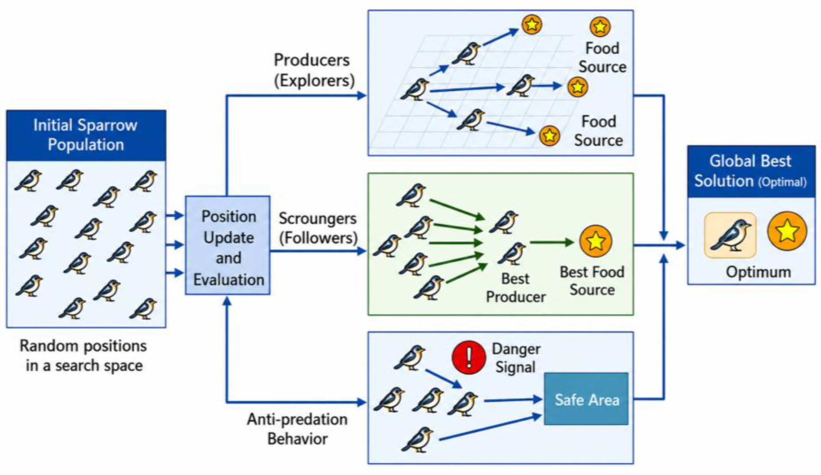
Random Forest (RF) is an ensemble learning algorithm that constructs multiple decision trees via bagging and random subspace methods [22]. By averaging predictions across diverse base learners, RF achieves robust performance in complex regression tasks. To optimize the model’s hyperparameters, the Sparrow Search Algorithm (SSA) was employed. The SSA is a swarm intelligence optimizer inspired by sparrow foraging and anti-predatory behaviors, known for its strong global search capabilities [23]. In this study, the SSA was introduced to perform secondary optimization on the RF hyperparameters, which had been pre-screened via grid search. This aimed to identify the optimal parameter combination capable of characterizing the temperature management features throughout the cucumber cultivation cycle in solar greenhouses in the Lingyuan region. A flowchart for the SSA-optimized temperature simulation model is illustrated in Figure 2. First, the preliminary ranges of hyperparameters were determined through grid search. Subsequently, the iterative mechanism of the SSA was utilized to perform a global search within the parameter space, with the objective of minimizing the simulation error, ultimately determining the optimal RF model configuration for expert experience simulation.

2.5. Construction of the Temperature Prediction Model

2.5.1. Data Denoising and Decomposition Based on CEEMDAN-PE

Greenhouse environmental data often exhibit non-stationarity and high-frequency noise due to abrupt changes in light, external weather disturbances, and sensor measurement errors, which can directly affect the stability and accuracy of predictive models. To effectively extract meaningful signals while suppressing random noise, this study employed CEEMDAN for adaptive multi-scale decomposition of the raw temperature series, combined with Permutation Entropy (PE), to evaluate the complexity of each Intrinsic Mode Function (IMF) and distinguish noise from trend signals. Compared with conventional filtering or simple smoothing methods, this approach retains low-frequency trend information while removing high-frequency stochastic disturbances, thereby improving the learning efficiency and prediction accuracy of the model. This noise processing strategy is a key component enabling the CNN-BiLSTM-Attention model to achieve high-precision, multi-step greenhouse temperature prediction.

To address non-stationarity and extract multi-scale features, a three-stage decomposition-optimization approach was implemented:

(1)

Adaptive Decomposition (CEEMDAN): The raw temperature sequence was decomposed into Intrinsic Mode Functions (IMFs) and a residual (RES) component. CEEMDAN was utilized to mitigate mode mixing by incorporating adaptive white noise, effectively deconstructing the signal into various characteristic scales [24].

(2)

Complexity Evaluation (PE): Permutation Entropy (PE) quantitatively assessed the randomness of each IMF [25]. High PE values indicated stochastic noise, while low PE values indicated distinct physical patterns and structural trends, providing a numerical basis for reconstruction.

(3)

Denoising and Reconstruction: A PE threshold of 0.6 was applied to categorize IMFs into noise, fluctuation, and trend terms. Noise components were removed, and the remaining IMFs were superimposed with the RES term to form the denoised sequence. Merging components with similar scales provided stable, high-quality input features for the neural network (Section 2.5.2).

2.5.2. Architecture of the Hybrid Prediction Model

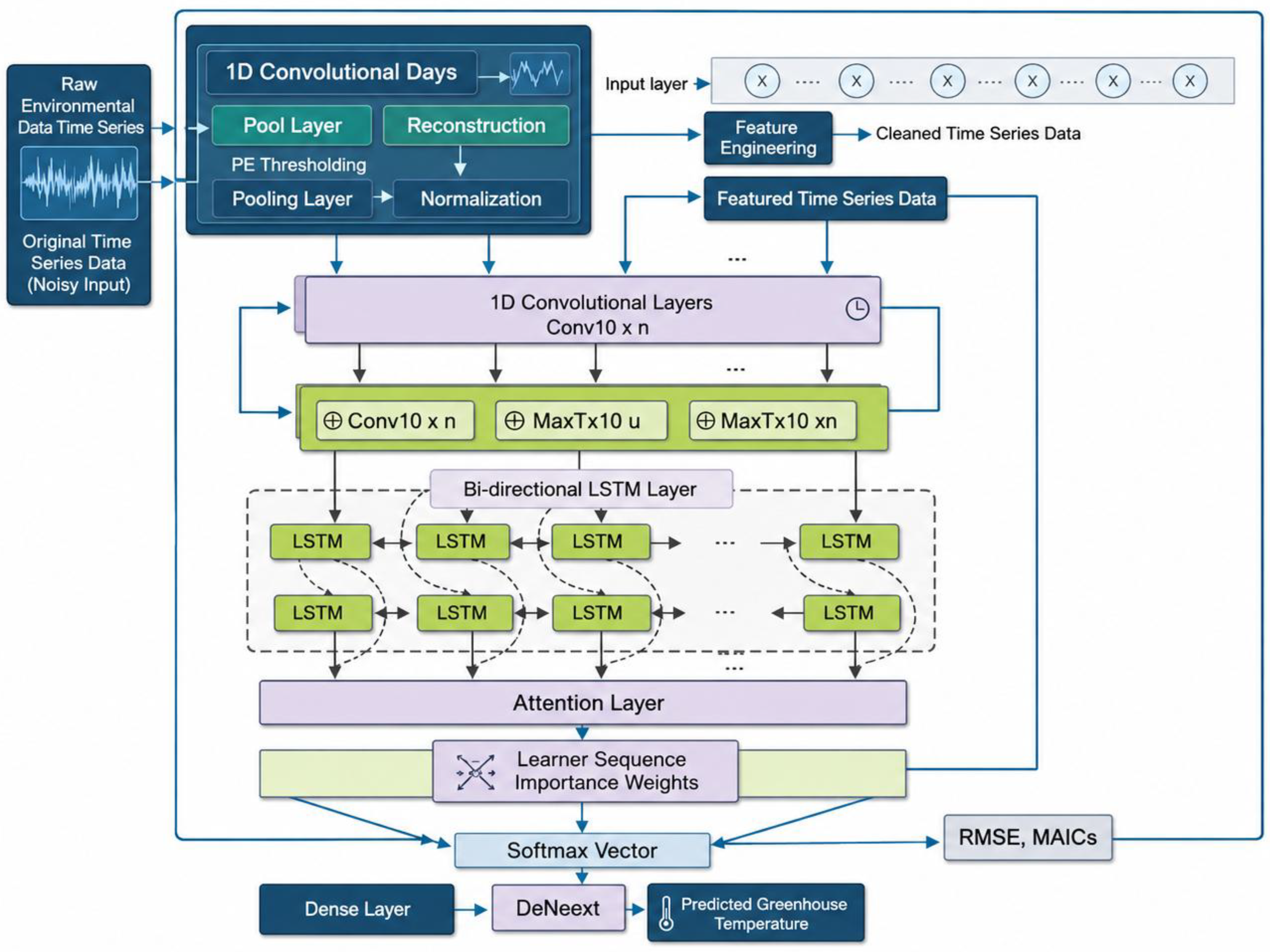
The hybrid prediction model developed in this study (Figure 3) was constructed by vertically stacking a CNN spatial feature extraction layer, a BiLSTM temporal feature learning layer, and an Attention weight allocation layer. The model achieves high-precision prediction of the reconstructed sequences from Section 2.5.1 through the following design logic:

(1)

CNN Spatial Transformation: Unlike conventional inputs, the CEEMDAN-decomposed multi-component matrix is processed via 1D-CNN kernels. This layer performs local perception across IMF components, extracting implicit spatial correlations and compressing high-dimensional data into dense feature vectors.

(2)

BiLSTM Bidirectional Recurrence: To overcome the limitations of unidirectional LSTM, a bidirectional mechanism captures temperature patterns via forward hidden layers and environmental fluctuation compensation via backward layers [26]. Concatenating these states enables the model to learn complex temporal dependencies within high-lag greenhouse environments.

(3)

Attention-based Weighted Integration: An Attention mechanism [27] serves as a feature filter to assign weights to BiLSTM outputs. During abrupt transitions (e.g., sunrise/sunset), it prioritizes critical time nodes and specific IMFs, allowing the model to capture non-linear disturbances rather than simple historical averaging.

2.5.3. Ablation Study Design for the Hybrid Prediction Model

An ablation study is a standard experimental method in the field of machine learning and hybrid modelling, aimed at analyzing the impact of specific components on overall performance by systematically removing or modifying parts of the model. This approach facilitates a deeper understanding of the function and significance of each component, thereby enabling the optimization of the model structure [28]. To further verify the effectiveness and necessity of each component in the proposed CNN-BiLSTM-Attention hybrid model for greenhouse temperature prediction, the following ablation experiments were designed:

(1)

Validation of CEEMDAN-PE denoising effect: The model (a standalone CNN-BiLSTM-Attention model) was constructed using the raw, un-decomposed sequences as input. By comparing this with the full model, the role of multi-scale feature extraction (described in Section 2.5.1) in mitigating signal non-stationarity was evaluated.

(2)

Validation of CNN spatial extraction capability: The model was developed by removing the CNN layer and directly inputting the components into BiLSTM. This was used to verify the necessity of convolutional operations for feature fusion and dimensionality reduction of multi-dimensional IMF components.

(3)

Validation of BiLSTM bidirectional learning advantages: The model was constructed by replacing BiLSTM with unidirectional LSTM. This comparison aimed to validate the capability of the “concatenating forward and backward hidden states” (described in Section 2.5.2) in capturing temperature responses in high-lag greenhouse environments.

(4)

Validation of the Attention weight allocation mechanism: The model was developed by removing the Attention mechanism layer. By comparing the error variations during periods of drastic temperature changes (e.g., after sunrise), the improvement effect of adaptive weight adjustment in capturing instantaneous environmental disturbances was verified.

2.6. Model Evaluation Indices

Root mean square error (RMSE), mean absolute percentage error (MAE), and the coefficient of determination (${\mathrm{R}}^2$) were selected as performance indices. Lower RMSE and MAPE values indicate superior prediction performance, while an ${\mathrm{R}}^2$ value closer to 1 signifies a better fit of the model. The specific calculation formulae are given by Equations (3)–(5):

$$RMSE = \sqrt{{\displaystyle \frac{{{\displaystyle \sum }}_{i=1}^n{\left(y_i - f\left(x_i\right)\right)}^2}{n}}}$$

(3)

$$MAE={\displaystyle \frac{1}{n}}{\displaystyle \sum }_{i=1}^n\left|y_i-f\left(x_i\right)\right|$$

(4)

$$R^2=1-{\displaystyle \frac{{{\displaystyle \sum }}_{i=1}^n{\left(y_i-\overline{y}\right)}^2}{{{\displaystyle \sum }}_{i=1}^n\left(y_i-\overline{y}\right)}}$$

(5)

where $\mathit{n}$ represents the number of samples that the model simulates or predicts, ${\mathit{x}}_{\mathit{i}}$ represents the measured value of the ambient temperature in the greenhouse, $y_i$ represents the model’s simulated or predicted values, and $\overline{\mathrm{y}}$ represents the mean of the measured values.

2.7. Formulation of the MPC-Oriented Theoretical Decision Framework

2.7.1. Mathematical Formulation and Logic

In this study, the MPC module was formulated as a theoretical decision framework rather than an online controller. The available dataset mainly contained environmental measurements, including indoor and outdoor climate variables, but did not include continuous actuator operation records, such as ventilation window opening, thermal curtain position, or heating power. Therefore, this section focuses on the mathematical coupling between the expert reference trajectory and the multi-step prediction model.

In addition, greenhouse air temperature is strongly coupled with other microclimate variables, particularly relative humidity and vapor pressure deficit (VPD). In the present study, relative humidity, CO₂ concentration, light intensity, soil temperature, soil moisture, and outdoor meteorological variables were included as input variables of the prediction model to characterize the coupled greenhouse environment. However, the current MPC-oriented framework uses air temperature as the main controlled output. Simultaneous temperature–humidity–VPD control was not experimentally implemented because continuous actuator operation data for ventilation, heating, humidification, or dehumidification were not available. Therefore, the proposed framework should be regarded as a temperature-oriented MPC decision framework with potential extension to multivariable microclimate control.

Model Predictive Control (MPC) is an advanced control strategy based on receding horizon optimization and feedback correction. It is capable of explicitly handling optimization problems in multivariable, non-linear, and constrained dynamic systems, making it highly suitable for control objects such as solar greenhouses, which are characterized by a slow time-varying nature, strong coupling, and environmental disturbances.

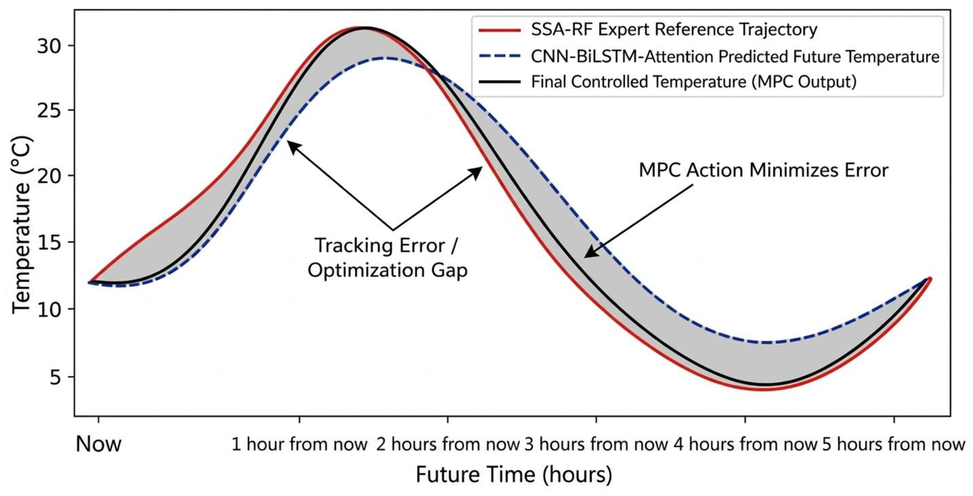
In this study, the core principle involves utilizing the prediction model to perform multi-step forecasting of future system behavior and generating optimal control commands for the current time step by solving an optimization problem within a finite time horizon [29]. The previously constructed high-precision temperature prediction model (CEEMDAN-PE-CNN-BiLSTM-Attention) and the expert-experience-based simulator (SSA-RF) were organically integrated and embedded into the MPC framework. The objective was to establish a theoretical decision-making basis for future closed-loop greenhouse temperature regulation, with emphasis on proactive prediction and control smoothness (Figure 4).

The optimization objective function $J$ considers temperature tracking accuracy and the smoothness of actuator actions. The second term penalizes the control increment rather than direct energy consumption. The control increment $\mathsf{\Delta }u$ represents the change in actuator commands between two adjacent control moments. Penalizing $\mathsf{\Delta }u$ can reduce frequent actuator switching and mechanical wear. However, direct energy consumption was not measured in this study.

To clarify the practical implications of $\mathsf{\Delta }u$ in the cost function, the following explanation and optional energy conversion formula are provided, highlighting its relationship to actual actuator operation and energy consumption.

In the proposed MPC cost function, $\mathsf{\Delta }u$ represents the incremental change of each actuator command between consecutive time steps. Physically, $\mathsf{\Delta }u$ corresponds to the additional energy consumption or mechanical effort required to adjust actuator states, such as heating power changes, ventilation window movements, or shading ratio adjustments. Penalizing $\mathsf{\Delta }u$ in the cost function does not imply maintaining the control input u constant. Instead, it aims to limit abrupt fluctuations in actuator commands, reducing energy spikes and mechanical wear while still allowing the system to track the expert reference temperature trajectory accurately.

This design is expected to support smoother actuator operation, reduce unnecessary control fluctuations, and provide a basis for improving energy efficiency and prolonging the service life of mechanical components in future implementation. Optionally, the relationship between $\Delta u$ and energy consumption can be quantified as:

$$E_{step} = \eta \cdot \mid \mathsf{\Delta }u\mid$$

(6)

where $E_{\mathrm{step}}$ is the energy associated with the incremental change and $\eta$ is a conversion factor representing actuator power-to-energy mapping. This explicit physical interpretation clarifies the engineering significance of minimizing $\mathsf{\Delta }u$ in the MPC formulation.

$$\underset{u}{\min }J=J_{error}+J_{energy}$$

(7)

The temperature tracking item measures the deviation from the predicted value and the expert reference value:

$$J_{error} ={\displaystyle \sum }_{i=1}^{ N_p}Q\cdot {\left[\widehat{T}(k + i|k) - T_{ref}\left(k + i\right)\right]}^2$$

(8)

The range of action of the incremental term is controlled to constrain the actuator: ${\mathrm{J}}_{\mathrm{energy}}$

$$J_{energy}={\displaystyle \sum }_{j=0}^{N_c-1}R\cdot {\left[\mathsf{\Delta }\mathrm{u}(k+j|k)\right]}^2$$

(9)

where k is the current discrete moment; $N_p$ is the length of the predicted time series (prediction horizon); $N_c$ is the control timing length; i is a subscript for predicting step length, which represents the ith point in time within the prediction horizon; $J$ (control step subscript) represents the jth action point in the control horizon; and u is a control variable/control input.

$\widehat{T}(k+i|k)$ is the predicted value of greenhouse temperature in the future from the hybrid prediction model (Section 2.5).

$T_{ref}\left(k+i\right)$ is the reference track of expert experience generated by the SSA-RF simulator (Section 2.4).

$\mathsf{\Delta }u(k+j|k)$ is the control increment, that is, the difference between the action instructions of the actuator (such as roller shutters and vents) at the two moments before and after.

Q and R are the error weight matrix and the control weight matrix, respectively, which are used to balance “temperature control accuracy” and “mechanical loss”.

The balance between temperature control accuracy and actuator protection is determined by the relative magnitudes of Q and R. A larger Q increases the penalty for the deviation between the predicted temperature and the expert reference trajectory, leading to more aggressive control actions and higher tracking accuracy. However, this may also cause frequent actuator adjustments. In contrast, a larger R increases the penalty on the control increment $\mathsf{\Delta }u$, thereby suppressing abrupt changes in actuator commands and reducing frequent start–stop operations, but it may also slow down the response to temperature deviations. Therefore, Q and R should not be interpreted independently. Instead, their relative ratio determines whether the controller prioritizes temperature tracking or actuator smoothness. In practical implementation, the weighting coefficients should be selected according to crop temperature tolerance, actuator specifications, and the acceptable trade-off between regulation accuracy and mechanical wear.

2.7.2. Constraint Design

When optimizing the objective function in Section 2.7.1, the physical limits and operational stability of the greenhouse actuator (e.g., ventilation window opening, shading net ratio) must be considered [30]. We set the following constraint equation.

$$u_{min} \le u\left(k+j\right) \le u_{max}$$

(10)

$${\mathsf{\Delta }\mathrm{u}}_{\min } \le \mathsf{\Delta }\mathrm{u}\left(\mathrm{k} + \mathrm{j}\right) \le {\mathsf{\Delta }\mathrm{u}}_{\max }$$

(11)

Variable Explanation and Physical Significance: Actuator amplitude constraints $\left(u\right)$ ${\mathrm{u}}_{\min } \mathrm{and} {\mathrm{u}}_{\max }$ represent the minimum and maximum control boundaries of the actuator, respectively. For example, the ventilation window opening is limited to between 0 (fully closed) and 100% (fully open). Action incremental constraints $\left(\mathsf{\Delta }u\right)$ $\mathsf{\Delta }{u}_{min} \mathrm{and} \mathsf{\Delta }{u}_{max}$ represent the maximum allowable change in the actuator per unit of time. These constraint are set to prevent the stepper motor from making frequent and large movements, thereby reducing mechanical losses and suppressing system overshoot. Time domain range: The above constraints must be satisfied in the entire control time domain to ensure that each control sequence calculated by optimization is executable in engineering, $J\in \left[0,{\mathrm{N}}_{\mathrm{c}}-1\right]$. These constraints were introduced to describe the feasible operating range of greenhouse actuators in future MPC implementation. They were not used to claim experimentally verified actuator control performance in this study.

From the perspective of actuator protection, the constraint design follows a three-level logic. First, the amplitude constraint limits the actuator command within its physical operating range, preventing infeasible commands such as excessive ventilation window opening or heating power. Second, the rate-of-change constraint limits the maximum variation in actuator commands between two adjacent control moments, thereby reducing abrupt motor movement, frequent switching, and mechanical wear. Third, in future online implementation, a dead-band or minimum switching interval can be introduced to further avoid unnecessary actuator start–stop operations when the temperature deviation is within an acceptable agronomic tolerance range. In this study, the first two types of constraints were mathematically formulated, while the third type is discussed as a future engineering extension because continuous actuator operation records were not available.

2.7.3. Rolling Optimization and Feedback Correction Mechanism

In the proposed MPC-oriented framework, the optimal control sequence is designed to be solved through rolling optimization in future online implementation [31]. Different from traditional global optimization, MPC only solves optimal control instructions in the future period at the current moment. The specific implementation steps are as follows:

Step 1: Real-time state acquisition and error compensation (feedback correction). In future online implementation, at the k-th moment, the actual greenhouse temperature can be obtained through sensors ${\mathrm{T}}_{\mathrm{act}}\left(\mathrm{k}\right)$. The actual value is used to feedback and correct the output of the hybrid prediction model in Section 2.5, and the current prediction error is calculated as $e \left(k\right)=T_{act}\left(k\right)-\widehat{T}(k|k-1)$. By compensating for errors, deviations caused by model mismatch or random environmental disturbances, such as instantaneous winds or personnel entry and exit, can be reduced, thereby providing a more accurate starting state for the optimization of the next period.

Step 2: Based on the corrected current system state and subject to the physical constraints described in Section 2.7.2, the quadratic programming (QP) algorithm can be adopted to solve the objective function in real time in future online implementation, thereby obtaining the optimal control sequence.

$$U^{*}\left(k\right)=[\mathsf{\Delta }{u}^{*}(k|k),\mathsf{\Delta }{u}^{*}(k+1|k),\dots ,\mathsf{\Delta }{u}^{*}(k+N_c-1|k){]}^T$$

(12)

where each $\mathsf{\Delta }{u}^{*}$ represents the optimal action increment of actuators (e.g., roller shutters, vents) at different moments in the future.

Step 3: Control the command issuance and time domain scrolling. According to the basic principle of MPC, the system would apply only the first control $\mathsf{\Delta }{u}^{*}(k|k)$ increment in the optimal sequence to the greenhouse actuator in future online implementation. At the next sampling moment $k+1$, the predicted time domain would be shifted forward by one step, and the system would re-acquire the environmental state and repeat the optimization process. This receding-horizon mechanism provides the controller with robustness against disturbances and flexibility for dynamic adjustment.

3. Results and Analysis

3.1. Correlation Analysis and Feature Selection of Environmental Variables

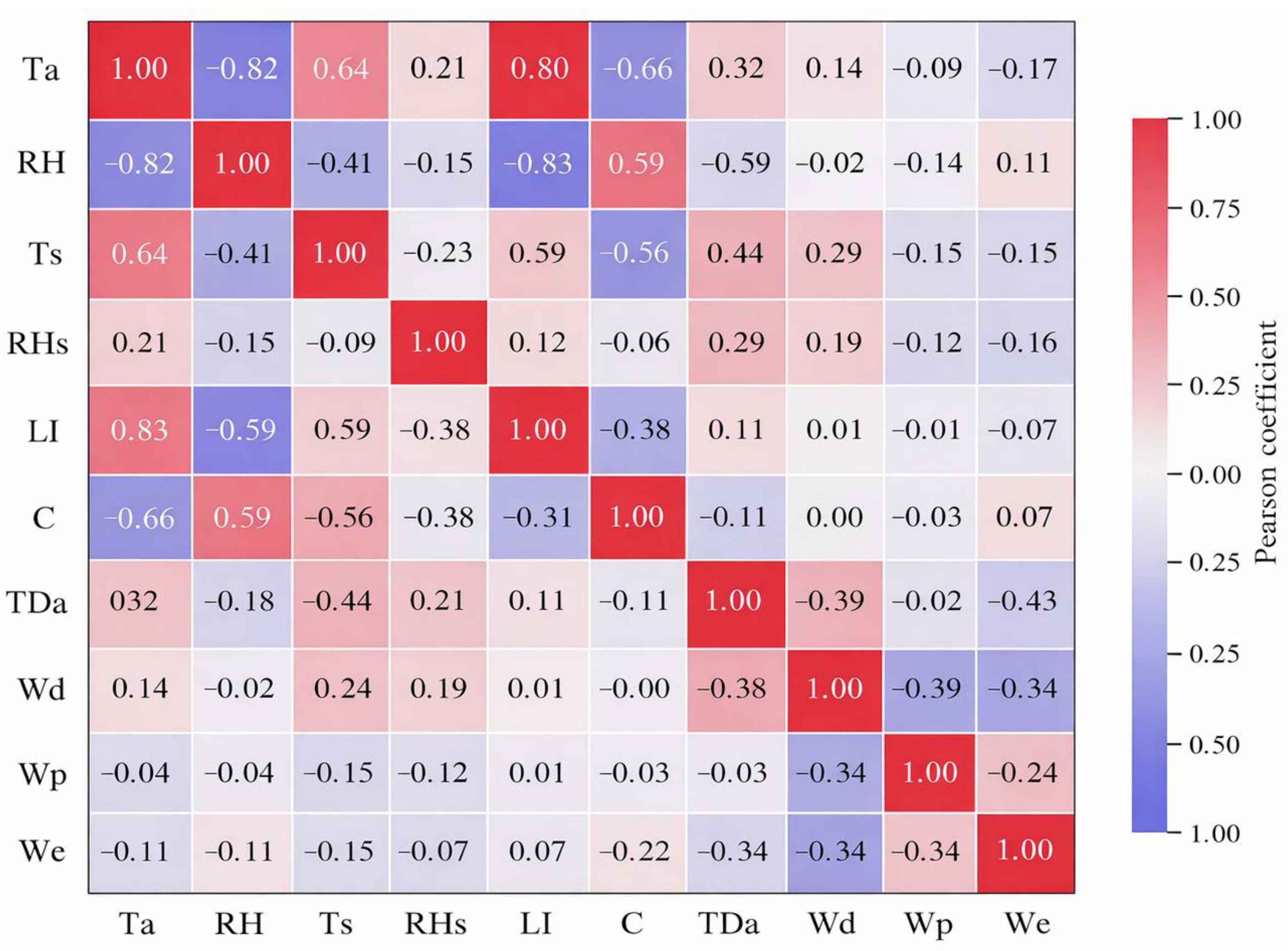
To construct an efficient and interpretable prediction model, environmental variables related to greenhouse air temperature were first analyzed. Pearson correlation analysis was used as an auxiliary method to provide an intuitive understanding of the linear relationships between environmental variables and greenhouse air temperature. It should be noted that Pearson correlation analysis was not used as the sole basis for final feature selection because greenhouse microclimate variables usually exhibit non-linear and coupled relationships. Therefore, RF feature importance ranking was further adopted as the primary criterion for determining the final input variables.

As shown in Figure 5, Pearson correlation analysis provided a preliminary linear correlation pattern among the environmental variables. Greenhouse air temperature showed relatively strong correlations with air humidity, light intensity, CO₂ concentration, and soil temperature, with most correlation coefficients exceeding 0.6. The absolute correlation coefficient between greenhouse air temperature and relative humidity was the highest, reaching −0.82. Moderate correlations were also observed between greenhouse air temperature and daily average outdoor temperature and soil moisture. In contrast, weather conditions, wind speed, and wind direction showed relatively weak linear correlations with greenhouse air temperature.

These results indicate that Pearson correlation analysis can provide useful preliminary evidence for identifying variables related to greenhouse air temperature. However, because Pearson analysis only reflects linear relationships, it may not fully describe the non-linear interactions and coupling effects among greenhouse environmental variables.

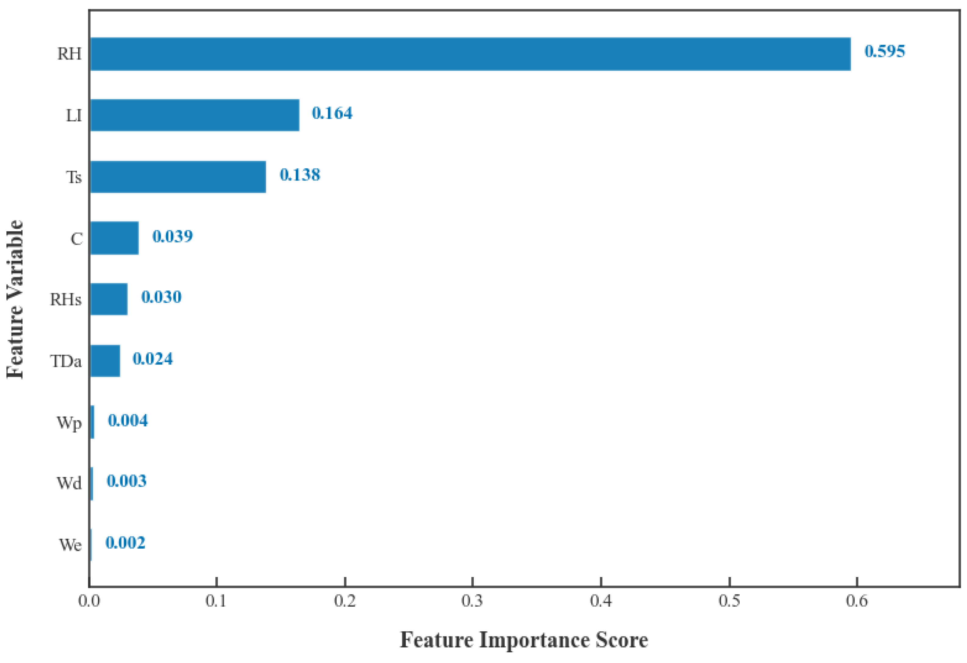
To further overcome the limitations of Pearson correlation analysis, RF feature importance ranking was used as the main basis for final feature selection. As shown in Figure 6, air humidity, light intensity, and soil temperature received relatively high importance scores. Although the importance scores of CO₂ concentration, soil moisture, and daily average outdoor temperature were lower, these variables still contributed to the prediction of greenhouse air temperature. In contrast, wind direction, wind speed, and weather conditions contributed less than 1% to the prediction task.

Therefore, based mainly on the RF feature importance ranking and supported by the Pearson correlation results, indoor humidity, light intensity, soil temperature, CO₂ concentration, soil moisture, and daily average outdoor temperature were selected as the input variables for the subsequent prediction models.

In addition, considering the thermal inertia of solar greenhouses, the selected variables were not used only as current time inputs. Instead, they were organized into temporal input windows before being introduced into the prediction model. This design allowed the model to learn the delayed response of greenhouse air temperature to previous changes in light intensity, outdoor temperature, humidity, and other environmental factors. Therefore, the final input design considered both feature importance and temporal dependence.

3.2. Performance of the SSA-RF Expert-Experience-Based Simulator

To digitize high-yield management expertise, the performance of the baseline Random Forest (RF) model was compared with that of the SSA-optimized RF model. As summarized in

Table 5. Test and verification error of the SSA-RF optimization model.

Data Set	Model	RMSE	MAE	R2
Test set	RF model	1.236	0.781	0.969
	SSA-RF model	1.081	0.586	0.976
Validation set	RF model	3.438	2.258	0.734
	SSA-RF model	1.554	1.029	0.946

, the RMSE and MAE of the SSA-RF model on the test set were reduced by 12.5% and 25.0%, respectively, compared to the baseline RF, while the ${\mathrm{R}}^2$ improved to 0.976. On the independent validation set, which represents the generalization capability of the model, the advantages were even more pronounced: the RMSE and MAE decreased by more than 54%, and the ${\mathrm{R}}^2$ increased from 0.734 to 0.946.

The SSA identified the optimal parameters to maximize the RF model’s generalization, ensuring precise temperature trend tracking. These results indicate that the SSA-RF model successfully quantified the “timely and moderate” environmental regulation logic inherent in high-yield farming data. The generated temperature sequence provides an agronomic reference trajectory for subsequent optimal control.

3.3. Performance of the Hybrid Prediction Model

3.3.1. Effects of Denoising and Decomposition

The raw temperature sequence was decomposed into 14 IMF components and one residual term using CEEMDAN. By calculating the Permutation Entropy (PE), it was observed that the high-frequency components IMF1–2 (PE > 2.3) contained significant random noise, while the low-frequency components IMF6–14 (PE < 1.25) carried the primary trend information. Based on the PE values, IMFs with similar complexity were reconstructed into four sub-sequences: high-frequency, intermediate-frequency, low-frequency, and trend terms (

Table 6. Arrange entropy of each eigenmode function.

Frequency	IMF	PE
	IMF1	2.573
High Frequency	IMF2	2.385
	IMF3	1.989
	IMF4	1.611
Intermediate Frequency	IMF5	1.364
	IMF6	1.250
	IMF7	1.162
	IMF8	1.093
	IMF9	1.057
Low Frequency	IMF10	1.032
	IMF11	1 014
	IMF12	1.005
	IMF13	1.002
	IMF14	0.999
	Res	0.003

).

The reconstruction process achieved signal–noise separation and data dimensionality reduction. High-frequency components were removed to minimize interference during model training, while low-frequency trends were preserved to ensure the stability of long-term predictions. This provided a cleaner and more structured input for the subsequent prediction model to handle non-stationary and noisy greenhouse time-series data.

To quantify the contribution of CEEMDAN-PE denoising to model performance, we compared the predictive results of the LSTM models with and without CEEMDAN-PE preprocessing (

Table 7. Quantitative evaluation of LSTM models with and without CEEMDAN-PE denoising. CEEMDAN-PE improves prediction accuracy by reducing RMSE and MAE and increasing R².

Model	Prediction Step Size/Time	RMSE	MAE	R2
LSTM	3/15 min	1.770	1.328	0.951
	6/30 min	2.036	1.532	0.935
CEEMDAN-PE-LSTM	3/15 min	1.748	1.308	0.952
	6/30 min	2.014	1.412	0.936

). The results show that after CEEMDAN-PE denoising, the 15 min prediction RMSE decreased from 1.770 to 1.748 (1.2% reduction), MAE decreased from 1.328 to 1.308, and R² increased from 0.951 to 0.952. For the 30 min prediction, RMSE decreased from 2.036 to 2.014 (1.1% reduction), MAE decreased from 1.532 to 1.412, and R² increased from 0.935 to 0.936. These results demonstrate that noise processing significantly improves the model’s predictive accuracy under non-stationary conditions, particularly during rapid changes in light and temperature. The denoised input provides higher-quality features for the CNN-BiLSTM-Attention model, enabling more accurate multi-step temperature forecasting.

3.3.2. Ablation Study and Model Comparison

Prior to input into the CNN-BiLSTM-Attention hybrid architecture, the raw temperature series undergoes CEEMDAN-PE denoising and decomposition (Section 2.5.1). This step separates high-frequency stochastic noise from low-frequency trend components, effectively reducing random fluctuations while retaining meaningful temporal patterns. By providing the hybrid model with clean, structured inputs, CEEMDAN-PE ensures that both the CNN spatial extraction and BiLSTM temporal learning layers can capture relevant environmental dynamics with higher fidelity. This preprocessing step is crucial for enhancing the model’s predictive accuracy, especially under non-stationary greenhouse conditions where abrupt environmental changes occur.

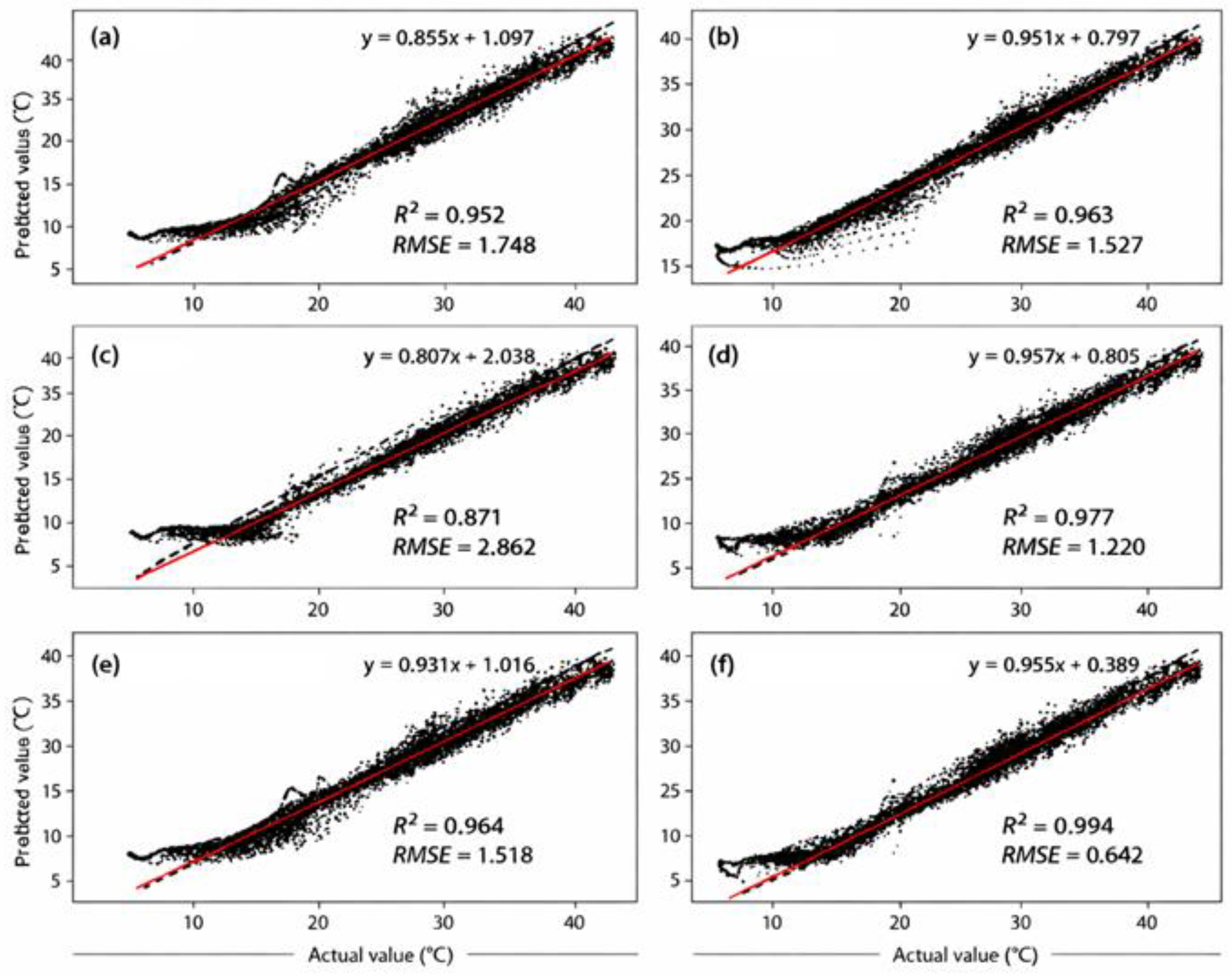
For a prediction horizon of three steps (representing a 15 min temperature forecast), the scatter plots of predicted versus actual values are shown in Figure 7. Following multiple rounds of testing, the various models in the ablation study exhibited distinct predictive performances. The hybrid CNN-BiLSTM-Attention model, established after temporal denoising, demonstrated a significantly lower RMSE compared to the other models. Furthermore, it achieved the highest coefficient of determination $\left(R^2=0.994\right)$, indicating that its explanatory power and fitting degree were superior to those of the alternative models.

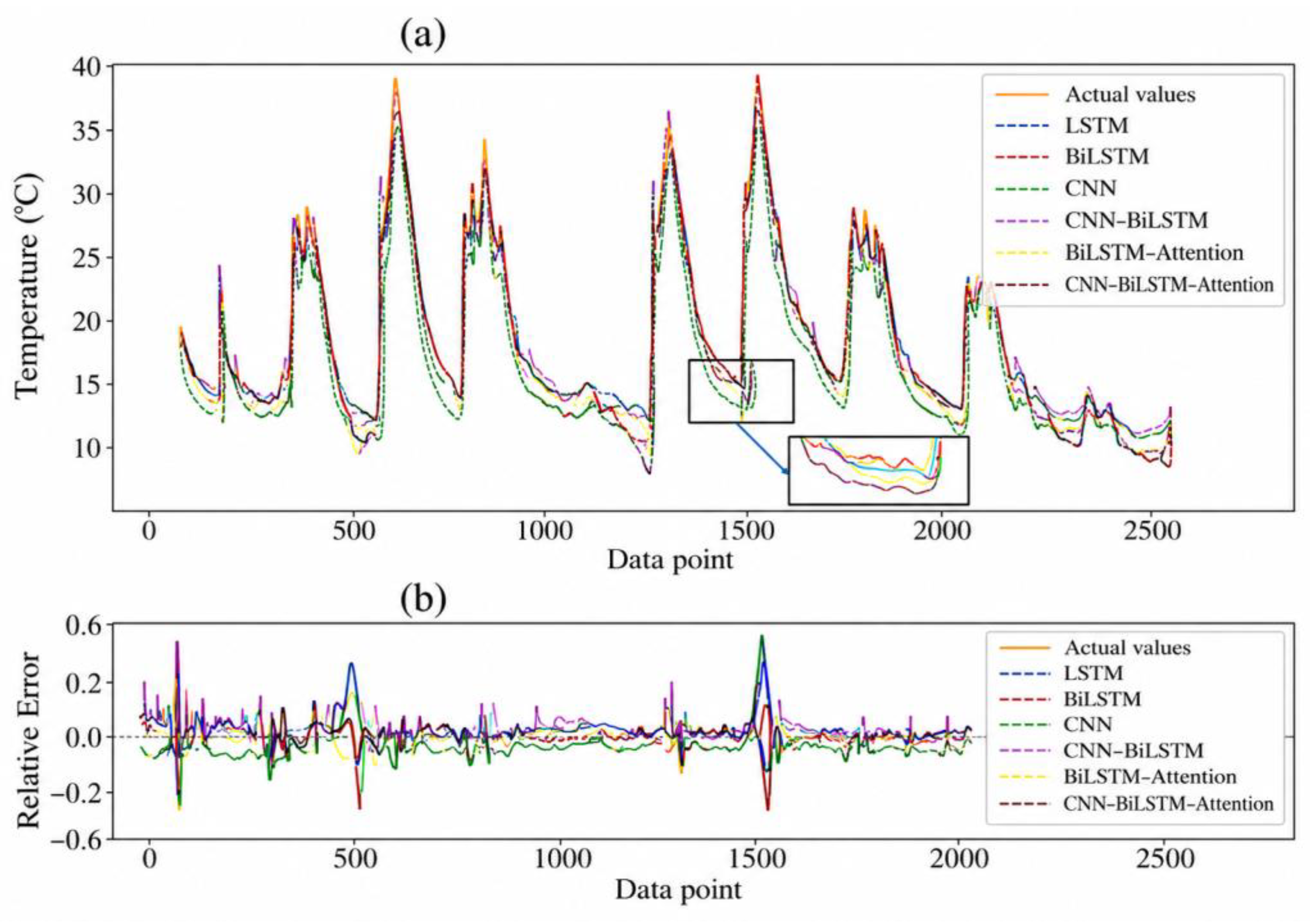
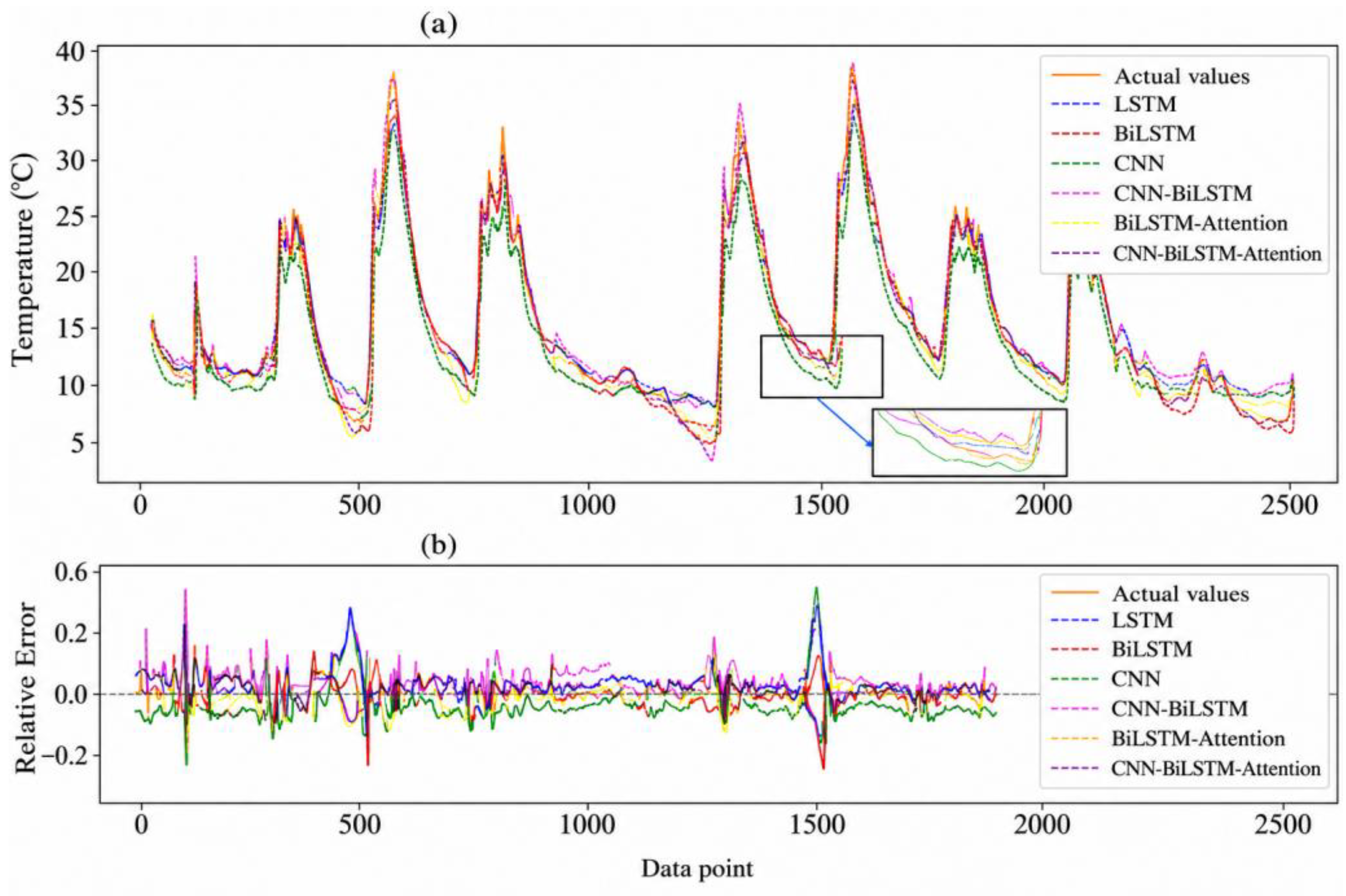
The comparison of predictive performance and relative error distributions for the 15 min forecast across all models is illustrated in Figure 8. The standalone models generally exhibited larger errors and poor fitting degrees. In contrast, the CNN-BiLSTM-Attention model developed in this study demonstrated superior fitting performance, aligning most closely with the actual values. Furthermore, its relative error distribution remained remarkably smooth and stable, indicating robust predictive performance.

Table 8. Prediction performance metrics (RMSE, MAE, R²) of ablation component models for the 3-step (15 min) forecast.

Model	RMSE	MAE	R2
LSTM	1.748	1.308	0.952
BiLSTM	1.662	1.284	0.956
CNN	2.862	2.580	0.871
CNN-BiLSTM	1.220	0.815	0.977
BiLSTM-Attention	1.518	1.176	0.964
CNN-BiLSTM-Attention	0.642	0.460	0.994

summarizes the RMSE, MAE, and R² values for all ablation component models in the three-step (15 min) prediction. The full CNN-BiLSTM-Attention model achieves the lowest errors and highest R², while removing CNN, BiLSTM, or Attention reduces accuracy, demonstrating the contribution of each module.

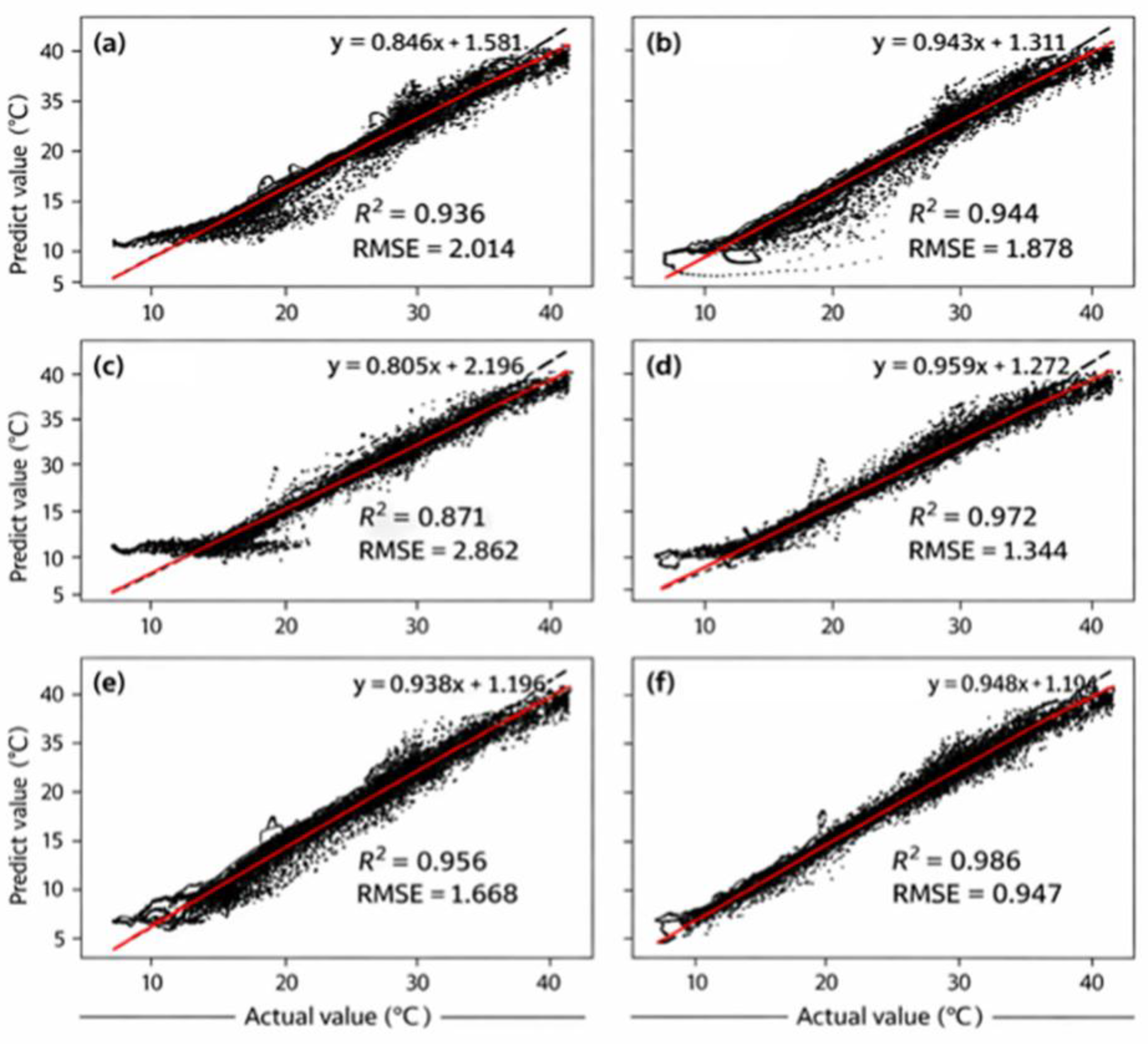
For a prediction horizon of six steps (representing a 30 min temperature forecast), a longer-term prediction experiment was conducted to align with the practical requirements of solar greenhouse production. According to the scatter distributions presented in Figure 9, the hybrid CNN-BiLSTM-Attention model consistently exhibited superior predictive performance. Its RMSE was significantly lower than those of the baseline models, achieving a maximum ${\mathrm{R}}^2$ of 0.947.

The performance comparison and relative error distributions for the 30 min forecast across all models are illustrated in Figure 10. The results indicate that the developed model maintains high predictive precision for the subsequent 30 min horizon, both during the stable nocturnal phase and under conditions of drastic temperature fluctuations during the daytime.

Table 9. Prediction performance metrics (RMSE, MAE, R²) of ablation component models for the 6-step (30 min) forecast.

Model	RMSE	MAE	R2
LSTM	2.014	1.412	0.936
BiLSTM	1.933	1.379	0.941
CNN	2.862	2.501	0.871
CNN-LSTM	1.344	0.926	0.972
BiLSTM-Attention	1.668	1.282	0.956
CNN-BiLSTM-Attention	0.947	0.678	0.986

summarizes the RMSE, MAE, and R² values for all ablation component models in the six-step (30 min) prediction. The full CNN-BiLSTM-Attention model maintains superior performance. The ablated models show larger errors, especially the CNN-only and BiLSTM-only variants, highlighting the importance of all components for multi-step forecasting.

Generalization capability validation: The fully trained hybrid model was applied to an entirely new control greenhouse that was not included in the training dataset (

Table 10. Verification of the mixed model in the experimental greenhouse and the control greenhouse.

Greenhouse	Prediction Step Size/Time	RMSE	MAE	R2
Experiment with greenhouse 1	3/15 min	1.281	0.687	0.949
Experiment with greenhouse 2		1.774	0.940	0.920
Control greenhouse		1.700	0.903	0.932
Experiment with greenhouse 1	6/30 min	1.646	0.941	0.915
Experiment with greenhouse 2		2.164	1.222	0.881
Control greenhouse		2.007	1.402	0.892

). In the 15 min prediction task, the model achieved an RMSE of 1.700, an MAE of 0.903, and an ${\mathrm{R}}^2$ of 0.932. Although there was a slight decline in performance compared to the training greenhouse, the results remained within the high-precision range. This effectively demonstrates that the CNN-BiLSTM-Attention model has captured the universal physical dynamics of the greenhouse environment rather than noise specific to a single site, thereby exhibiting excellent transferability.

3.3.3. Relative Error Analysis

To quantitatively evaluate the predictive accuracy of the proposed models, the relative error (RE) was computed as follows:

$$RE\left(t\right) = {\displaystyle \frac{\left|T_{pred}\left(t\right) - T_{meas}\left(t\right)\right|}{T_{meas}\left(t\right)}}\times 100\%$$

(13)

where $Tpred\left(t\right)$ and $Tmeas\left(t\right)$ denote the predicted and measured greenhouse temperatures at time step t, respectively.

Quantitative Results: The mean relative error (Mean RE) and maximum relative error (Max RE) for the 15 min and 30 min prediction horizons are summarized in

Table 11. Relative error of different prediction models at 15 min and 30 min horizons.

Model	Prediction Horizon	Mean RE (%)	Max RE (%)
LSTM	15 min	1.36	4.12
BiLSTM	15 min	1.21	3.85
CNN-BiLSTM-Attention	15 min	0.63	1.98
LSTM	30 min	1.72	5.03
BiLSTM	30 min	1.48	4.55
CNN-BiLSTM-Attention	30 min	0.95	2.47

.

The maximum and mean relative errors were calculated as:

$$\mathrm{Max} \mathrm{RE} = \max \left(RE\left(t\right)\right)$$

(14)

$$\mathrm{Mean} \mathrm{RE} ={\displaystyle \frac{1}{N}}{\displaystyle \sum }_{t=1}^{N}RE\left(t\right)$$

(15)

where N is the total number of prediction samples.

Engineering Implications:

(1)

For the 15 min prediction, the CNN-BiLSTM-Attention model achieved a mean RE of 0.63% and a maximum RE below 2%, indicating high short-term prediction accuracy suitable for providing reliable input to MPC-based control.

(2)

For the 30 min prediction, the mean RE remained below 1%, demonstrating stable mid-term predictive performance.

(3)

In practical greenhouse operations, such low prediction errors indicate that the proposed prediction model can provide reliable information for future temperature-control decisions, potentially helping to maintain crop environments within target ranges and reduce unnecessary actuator adjustments.

(4)

Theoretical analysis suggests that prediction errors at this level may provide a reliable basis for future tracking of expert reference trajectories and for maintaining actuator increments (Δu) within feasible boundaries.

3.3.4. Computational Efficiency and Deployment Feasibility

Although the proposed hybrid model was trained on a workstation equipped with an RTX4080 GPU, practical greenhouse deployment only requires the inference stage rather than repeated model training. The online prediction task in this study was conducted at a 5 min sampling interval, and the forecasting horizons were 15 min and 30 min. Therefore, the real-time requirement of the proposed framework is relatively relaxed compared with millisecond-level industrial control systems.

In practical deployment, the trained model can be executed on an edge-computing gateway, an industrial PC, or a local greenhouse control terminal. The cloud or workstation can be used for offline model training and periodic model updating, whereas the local edge device only needs to perform data normalization, input window construction, and forward inference. This “offline training–edge inference” strategy can reduce the computational burden of the on-site controller while maintaining timely temperature prediction for MPC-oriented decision support.

Therefore, the present analysis demonstrates the feasibility of the deployment strategy at the framework level but does not replace hardware-level benchmarking. Future work will further evaluate inference latency, memory consumption, and model size on edge devices and apply model compression, pruning, quantization, or knowledge distillation to improve the applicability of the model in low-cost greenhouse controllers.

3.4. Illustrative Analysis of Input Constraints in the MPC-Oriented Framework

To further clarify the input constraint mechanism in the proposed MPC-oriented framework, this section describes how the control input u and its incremental change Δu can be constrained during future MPC implementation. It should be noted that the present dataset mainly contains greenhouse environmental measurements and does not include continuous actuator operation records, such as ventilation window opening, thermal curtain position, shading ratio, or heating power. Therefore, this section is intended to illustrate the constraint-handling logic of the proposed framework rather than to provide experimental validation of an online MPC controller.

In the proposed formulation, u represents the actuator command and Δu represents the change in actuator command between two adjacent control moments, as expressed by:

$$\Delta u\left(k\right) = u\left(k\right) - u\left(k - 1\right)$$

(16)

The amplitude constraint of u ensures that the calculated control command remains within the physical operating range of the actuator. The rate-of-change constraint of Δu is introduced to avoid abrupt actuator movement, frequent switching, and excessive mechanical wear. These constraints can be expressed as:

$$u_{min} \le u\left(k\right) \le u_{max}$$

(17)

$$\mid \Delta u\left(k\right)\mid \le \Delta u_{max}$$

(18)

Representative actuator constraints are given in

Table 12. Representative actuator constraints for illustrative MPC-oriented framework.

Actuator	umin	umax	Δumax
Ventilation window	0%	100%	10%/step
Heater	0 kW	5 kW	0.5 kW/step

. For example, the ventilation window opening can be constrained within 0–100%, and its maximum change can be limited to 10% per control step. Similarly, heater power can be constrained within 0–5 kW, with a maximum change of 0.5 kW per control step. These values are used to illustrate the engineering meaning of the constraint formulation and can be adjusted according to the specifications of actual greenhouse actuators.

To further clarify the trade-off between temperature control accuracy and actuator protection, the role of the weighting coefficients Q and R should be interpreted together with the actuator constraints. In the MPC-oriented objective function, Q penalizes the deviation between the predicted greenhouse temperature and the expert reference trajectory, whereas R penalizes the control increment Δu. Therefore, a larger Q tends to improve temperature tracking accuracy by allowing more active actuator adjustments, but it may also increase the switching frequency and mechanical burden of actuators. In contrast, a larger R suppresses abrupt changes in actuator commands and helps protect mechanical devices, but an excessively large R may slow down the response to temperature deviations. Thus, the proposed framework does not pursue temperature accuracy at all costs; instead, it aims to achieve a compromise between accurate temperature tracking and smooth actuator operation.

From the perspective of actuator protection, the constraint design follows a hierarchical logic. First, the amplitude constraint $u_{min} \le u \le u_{max}$ ensures that the calculated actuator command remains within the physical operating range of the device. Second, the rate-of-change constraint $\mid \mathsf{\Delta }u\mid \le \mathsf{\Delta }{u}_{max}$ limits the maximum adjustment between two adjacent control steps, thereby reducing abrupt motor movement and frequent start–stop operations. Third, in future online implementation, a dead-band or minimum switching interval can be further introduced when the temperature deviation remains within an acceptable agronomic tolerance range. This can prevent unnecessary actuator activation caused by small prediction fluctuations. In the present study, the first two constraint types were mathematically formulated, while the dead-band and minimum switching interval are discussed as future engineering extensions because continuous actuator operation records were not available.

As shown in

Table 13. Conceptual comparison of different weighting strategies in the MPC-oriented framework.

Strategy	Weight Setting	Expected Control Behavior	Temperature Tracking Accuracy	Actuator Protection
Aggressive tracking	High Q, low R	Rapid response to temperature deviations, with frequent actuator adjustments	High	Low
Balanced regulation	Moderate Q, moderate R	Compromise between temperature tracking and actuator smoothness	Moderate to high	Moderate to high
Conservative protection	Low Q, high R	Smooth actuator movement and reduced start–stop frequency, but slower response	Moderate or low	High

, different Q/R settings lead to different control tendencies. The balanced regulation strategy was adopted as the theoretical design principle of the proposed MPC-oriented framework. Under this strategy, the controller is expected to track the expert reference temperature trajectory while avoiding excessive actuator increments. However, because the present dataset did not include real actuator operation records, the optimal Q/R ratio and the actual reduction in actuator wear were not experimentally validated. Future studies will compare different Q/R settings using real actuator data and evaluate both temperature tracking error and actuator operation indicators, such as switching frequency, cumulative control variation, actuator running time, and energy consumption.

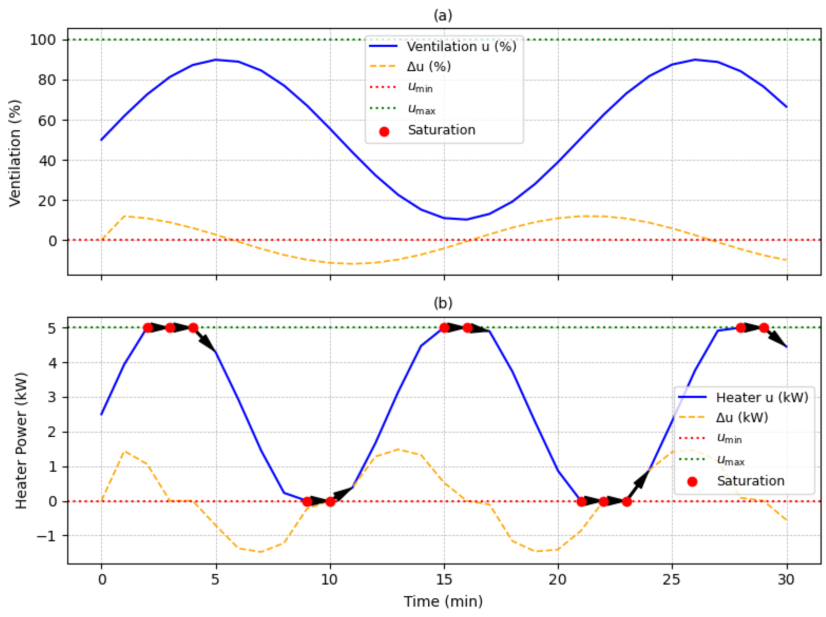
Based on the above constraint and weighting logic, Figure 11 provides a schematic illustration of the constrained control input and its incremental change. The upper and lower bounds define the feasible operating range of the actuator, while the Δu_max boundary limits the maximum change between adjacent control moments. When the actuator command approaches the upper or lower boundary, the amplitude constraint prevents physically infeasible commands. Meanwhile, the incremental constraint smooths the control trajectory and reduces abrupt fluctuations. Therefore, the proposed constraint design provides a physically executable basis for future MPC-based greenhouse temperature regulation.

It should be emphasized that Figure 11 and Table 13 are conceptual analyses rather than closed-loop control experiments or complete dynamic simulations. The actual saturation behavior, temperature tracking performance, actuator switching frequency, control energy consumption, and mechanical wear should be further verified using real actuator-operation data and greenhouse thermal dynamic models. Future work will integrate ventilation window opening, thermal curtain position, heating power, fan operation, and other actuator signals into a closed-loop MPC platform to quantitatively compare different Q/R weighting strategies and evaluate the control performance under practical production conditions.

4. Discussion

4.1. Analysis of Integrated Advantages

(1)

Necessity of the SSA optimization algorithm in the expert experience simulator. In constructing the expert experience simulator, the SSA was introduced to optimize the Random Forest (RF) model. Compared to traditional grid search [32] or random search methods, the swarm intelligence evolutionary mechanism of the SSA exhibits superior global search capabilities when navigating the high-dimensional, non-linear parameter spaces characteristic of greenhouse environments. In contrast to prior studies that relied on standalone machine learning models (e.g., BP neural networks, SVM) to simulate farmer interventions, which often fall into local optima and suffer significant precision loss under edge conditions like seasonal transitions, the SSA-RF demonstrated high robustness (${\mathrm{R}}^2 = 0.946$). This advantage stems from the SSA’s precise balancing of RF tree depth and feature subsets, effectively mitigating the “prediction smoothing” phenomenon at extreme values commonly observed in conventional RF models.

(2)

Mechanism of the hybrid prediction model in capturing multi-scale temporal features. Given the non-stationary nature of solar greenhouse temperature sequences, the CEEMDAN-PE decomposition scheme is critical for enhancing predictive precision. Unlike direct single-dimensional forecasting using LSTM or CNNs, this algorithm deconstructs the raw sequence into Intrinsic Mode Functions (IMFs) of varying frequencies. Physically, these correspond to “slow trends” (influenced by seasons and meteorology) and “rapid fluctuations” (driven by thermal blankets and ventilation fans). As evidenced in the ablation study (Section 3.3.2), models without PE-based restructuring exhibited significant lag when processing high-frequency noise. Compared to the EMD decomposition frequently used in similar research [33], the proposed scheme effectively circumvents the mode mixing problem.

(3)

Proactive nature and practicality of the MPC-oriented regulation framework. From a control-design perspective, integrating expert experience and prediction models within an MPC-oriented framework may help reduce the lag of traditional feedback control in future implementation [34]. While traditional greenhouse control relies primarily on “instantaneous error” adjustments, this study leverages the prediction model to provide a 30 min forecast. This logic mirrors the proactive behavior of experienced farmers, such as lowering thermal blankets ahead of a cold wave. Furthermore, compared to current Reinforcement Learning (RL)-based regulation schemes, the advantage of this framework lies in its constraint mechanism. While RL models often generate irrational control commands (e.g., frequent window toggling) during early training phases, this study incorporates control increment penalties into the MPC objective function. This is expected to improve temperature control precision while reducing unnecessary mechanical wear in future implementation.

4.2. Engineering-Oriented Modelling of Constraints and the Q/R Weighting Trade-Off

In the design of the integrated regulation framework, the introduction of constraints serves not only to ensure system safety but also to seek the optimal equilibrium between “temperature control precision” and “actuation efficiency.” By incorporating these hard constraints during the receding-horizon optimization stage, the generation of unreachable control commands under drastic weather fluctuations can be avoided in future implementation, thereby improving the physical compatibility between the regulation instructions and the underlying actuators [35]. Furthermore, the weight-based trade-off between Q and R provides a flexible configuration scheme for greenhouse management across different crop stages and climatic conditions. When crops are highly sensitive to temperature fluctuations, such as during the seedling stage or under extreme cold conditions, Q can be increased to improve temperature tracking accuracy. In contrast, when the crop has a wider temperature tolerance range or when the actuator is frequently switched under fluctuating weather conditions, R can be increased to suppress excessive control increments and protect mechanical devices. Therefore, the proposed MPC-oriented framework does not pursue temperature accuracy at all costs. Instead, it seeks a compromise between tracking the expert reference trajectory and maintaining smooth, physically feasible actuator operation. This provides a theoretical rationale for the weighting coefficient settings in Equations (8) and (9) [36].

4.3. Limitations and Future Work

While the developed MPC framework establishes a theoretical basis for intelligent solar greenhouse management, large-scale application requires further research in:

(1)

Computational Efficiency and Edge Deployment: Although the proposed model was trained on a high-performance workstation, practical greenhouse application mainly requires online inference. An “offline training–edge inference” strategy can be adopted in future deployment, where model training and updating are performed on a workstation or cloud server and the trained model is deployed on an edge-computing gateway, industrial PC, or local greenhouse control terminal. Future work will evaluate inference latency, memory consumption, and model size on low-power devices and apply model compression, pruning, quantization, and knowledge distillation to improve deployment feasibility [37].

(2)

Lag window Optimization: Although historical information was included through temporal window inputs, variable-specific lag lengths were not independently optimized. Future work will compare different lag structures to further improve prediction accuracy and interpretability.

(3)

Robustness and Adaptation: Integrate Recursive Least Squares (RLS) or online learning can be used to create a closed-loop feedback compensation, enhancing adaptability across diverse climates and structures [38].

(4)

Multivariable Control: The present study focused on temperature-oriented prediction and MPC formulation. However, greenhouse air temperature is closely coupled with relative humidity, crop transpiration, and VPD. A temperature-only control strategy may cause undesirable side effects, such as excessive humidity accumulation during low-temperature periods or excessively high VPD under strong solar radiation. Therefore, future work will extend the current framework from single-variable temperature regulation to coordinated temperature–humidity–VPD control by incorporating humidity-related actuator data, crop transpiration information, and water–heat coupling models. In this way, the MPC framework can further balance temperature tracking, humidity stability, crop physiological demand, and actuator smoothness.

This study has several limitations. First, the MPC framework was mathematically formulated but was not validated through an online closed-loop control experiment. This is because the current dataset did not include real-time actuator data, such as ventilation window opening, thermal curtain position, shading ratio, or heating power. Second, the objective function mainly penalizes temperature tracking error and control increments. Therefore, the current formulation reflects control smoothness and actuator stability rather than directly measured energy consumption. Third, this study focused on temperature prediction and expert reference trajectory generation. Future work should integrate actuator data, greenhouse thermal dynamics, and real-time control platforms to verify the proposed MPC-oriented framework under actual production conditions.

In addition, although the proposed framework theoretically balances temperature tracking accuracy and actuator protection through Q/R weighting and Δu constraints, the actual trade-off among tracking error, switching frequency, actuator wear, and energy consumption was not experimentally validated because continuous actuator operation data were unavailable.

5. Conclusions

This study developed an MPC-oriented temperature regulation framework for solar greenhouses by integrating an expert experience simulator and a hybrid multi-step temperature prediction model. The work was designed to address three key issues in greenhouse temperature management: the difficulty of digitizing experienced growers’ regulation strategies, the limited robustness of conventional prediction models under non-stationary greenhouse environments, and the lack of an explicit decision-making framework linking prediction results with future constrained control.

First, the SSA-RF expert experience simulator successfully transformed the temperature management logic of high-yield farmers into dynamic reference trajectories. Compared with the traditional RF model, the SSA-RF model achieved better simulation accuracy and generalization performance. On the test set, the SSA-RF model reduced the RMSE and MAE by 12.5% and 25.0%, respectively, and improved the R² to 0.976. On the independent validation set, the RMSE and MAE decreased by more than 54%, and the R² increased from 0.734 to 0.946. These results indicate that the SSA optimization strategy improved the ability of the RF model to capture non-linear expert regulation patterns and provided a reliable agronomic reference trajectory for subsequent MPC-oriented decision-making.

Second, the CEEMDAN-PE-CNN-BiLSTM-Attention hybrid prediction model showed clear advantages over conventional and ablated models. For the 15 min prediction horizon, the full hybrid model achieved an RMSE of 0.642, an MAE of 0.460, and an R² of 0.994, outperforming the LSTM, BiLSTM, CNN, CNN-BiLSTM, and BiLSTM-Attention models. For the 30 min prediction horizon, the model maintained high prediction accuracy, with an RMSE of 0.947, an MAE of 0.678, and an R² of 0.986. The ablation results confirmed that CEEMDAN-PE preprocessing, CNN spatial feature extraction, BiLSTM temporal learning, and the Attention mechanism each contributed to improving prediction performance. The relative error analysis further showed that the proposed model achieved mean relative errors of 0.63% for 15 min prediction and 0.95% for 30 min prediction, with maximum relative errors of 1.98% and 2.47%, respectively. These results demonstrate that the hybrid model can provide accurate and stable multi-step temperature forecasts for MPC-oriented regulation.

Third, the validated expert reference trajectory and prediction model were theoretically integrated into an MPC-oriented decision framework. The framework established a mathematical connection among expert reference temperature trajectories, multi-step prediction results, actuator constraints, and control increments. In addition, the roles of Q, R, and Δu were clarified to explain the trade-off between temperature tracking accuracy and actuator protection. The proposed constraint design provides a theoretical basis for avoiding physically infeasible actuator commands and reducing unnecessary control fluctuations in future online implementation.

Overall, this study contributes a complete technical path from expert knowledge digitization and high-precision temperature prediction to MPC-oriented decision formulation. The proposed framework has potential engineering value for intelligent greenhouse management because it combines agronomic experience, data-driven prediction, and constraint-aware control logic. It can support future development of real-time temperature regulation systems that are more proactive, interpretable, and compatible with actuator limitations than conventional rule-based control strategies.

However, the present study still has several limitations. The MPC module was formulated as a theoretical decision-making framework rather than a fully validated online closed-loop controller because continuous actuator-operation data were not available. Therefore, the actual control performance, actuator switching frequency, energy consumption, and mechanical wear reduction were not experimentally verified. In addition, the current framework focused mainly on temperature-oriented regulation, while coordinated temperature–humidity–VPD control remains to be further developed. Future studies should integrate real actuator data, greenhouse thermal dynamic models, humidity-related variables, and edge deployment tests to verify the proposed framework under practical production conditions and compare it with rule-based, PID, and other control strategies.

References

1. Parra-Lopez, C.; Ben Abdallah, S.; Garcia-Garcia, G.; Hassoun, A.; Sanchez-Zamora, P.; Trollman, H.; Jagtap, S.; Carmona-Torres, C. Integrating Digital Technologies in Agriculture for Climate Change Adaptation and Mitigation: State of the Art and Future Perspectives. Comput. Electron. Agric. 2024, 226, 109412. [Google Scholar] [CrossRef]
2. He, M.; Wan, X.; Liu, H.; Xia, T.; Gong, Z.; Li, Y.; Liu, X.; Li, T. Theory and Application of Sustainable Energy-Efficient Solar Greenhouse in China. Energy Convers. Manag. 2025, 325, 119394. [Google Scholar] [CrossRef]
3. Bezari, S.; Adda, A.; Merabti, S.; Oztekin, G. Artificial Neural Network Model for Microclimate Performance of Solar Greenhouse with Thermal Storage. Therm. Sci. 2025, 29, 3603–3614. [Google Scholar] [CrossRef]
4. Li, K.; Shi, J.; Hu, C.; Xue, W. The Intelligentization Process of Agricultural Greenhouse: A Review of Control Strategies and Modeling Techniques. Agriculture 2025, 15, 2135. [Google Scholar] [CrossRef]
5. Zhang, Y.; Xu, L.; Zhu, X.; He, B.; Chen, Y. Thermal Environment Model Construction of Chinese Solar Greenhouse Based on Temperature–Wave Interaction Theory. Energy Build. 2023, 279, 112648. [Google Scholar] [CrossRef]
6. Chen, S.; Liu, A.; Tang, F.; Hou, P.; Lu, Y.; Yuan, P. A Review of Environmental Control Strategies and Models for Modern Agricultural Greenhouses. Sensors 2025, 25, 1388. [Google Scholar] [CrossRef]
7. Mayne, D.Q.; Rawlings, J.B.; Rao, C.V.; Scokaert, P.O.M. Constrained Model Predictive Control: Stability and Optimality. Automatica 2000, 36, 789–814. [Google Scholar] [CrossRef]
8. Ghahremani, Y.; Maihami, V. Face Recognition Based on Deep Learning Convolutional Neural Network in Cloud Internet of Things Environment. SN Comput. Sci. 2025, 7, 48. [Google Scholar] [CrossRef]
9. Liu, W.; Han, T.; Wang, C.; Zhang, F.; Xu, Z. Predicting Indoor Temperature of Solar Green House by Machine Learning Algorithms: A Comparative Analysis and a Practical Approach. Smart Agric. Technol. 2025, 12, 101096. [Google Scholar] [CrossRef]
10. Morcego, B.; Yin, W.; Boersma, S.; Van Henten, E.; Puig, V.; Sun, C. Reinforcement Learning versus Model Predictive Control on Greenhouse Climate Control. Comput. Electron. Agric. 2023, 215, 108372. [Google Scholar] [CrossRef]
11. Jiang, S.Y.; Zhang, X.X.; Mo, Y.; Huang, Y.J. Research on Noise Reduction Method of Underwater Acoustic Signal Based on CEEMDAN Decomposition-Improved Wavelet Threshold. J. Phys. Conf. Ser. 2024, 2718, 012078. [Google Scholar] [CrossRef]
12. Zhang, D.; Du, W.; Yu, S.; Hong, Z.; Avirmed, D.; Li, M.; He, Y. Prediction of Sandstorm Moving Path in Mongolian Plateau Based on CNN-BiLSTM. Remote Sens. 2025, 17, 3006. [Google Scholar] [CrossRef]
13. Bai, X.; Zhang, L.; Feng, Y.; Yan, H.; Mi, Q. Multivariate Temperature Prediction Model Based on CNN-BiLSTM and RandomForest. J. Supercomput. 2025, 81, 162. [Google Scholar] [CrossRef]
14. Shi, P.; Tang, M.; Wang, Q.; Ma, X. Optimization of TCN-BiLSTM for Dissolved Oxygen Prediction Based on Improved Sparrow Search Algorithm. Sci. Rep. 2025, 15, 30790. [Google Scholar] [CrossRef]
15. Iddio, E.; Wang, L.; Thomas, Y.; McMorrow, G.; Denzer, A. Energy Efficient Operation and Modeling for Greenhouses: A Literature Review. Renew. Sustain. Energy Rev. 2020, 117, 109480. [Google Scholar] [CrossRef]
16. Bersani, C.; Fossa, M.; Priarone, A.; Sacile, R.; Zero, E. Model Predictive Control versus Traditional Relay Control in a High Energy Efficiency Greenhouse. Energies 2021, 14, 3353. [Google Scholar] [CrossRef]
17. Wang, B.; Wang, L.; Ma, Y.; Hou, D.; Sun, W.; Li, S. A Short-Term Load Forecasting Method Considering Multiple Factors Based on VAR and CEEMDAN-CNN-BILSTM. Energies 2025, 18, 1855. [Google Scholar] [CrossRef]
18. Quamer, A.; Asgari, N.; Pearce, J.M. Two-Stage Deep Learning Model for Non-Destructive Leaf Counting in Tomato Crops. Comput. Electron. Agric. 2026, 247, 111717. [Google Scholar] [CrossRef]
19. Yuan, Y.; Tang, X.; Li, H.; Lang, X.; Song, Y.; Yang, Y.; Zhou, Z. BiLSTM- and CNN-Based m6A Modification Prediction Model for circRNAs. Molecules 2024, 29, 2429. [Google Scholar] [CrossRef] [PubMed]
20. Lin, Z.; Wang, Y.; Fu, X.; Zou, Z.; Feng, L.; Fang, L.; Qing, X. Defect Localization and Quantification of Energy Transportation Pipeline Based on Multiscale 1DCNN and BiLSTM with Multidimensional Attention Mechanism. Energy 2026, 344, 139879. [Google Scholar] [CrossRef]
21. Lin, J.; Chen, Q.; Xue, B.; Rooney, J.S.; Zhang, M.; Lagutin, K.; MacKenzie, A.; Gordon, K.C.; Killeen, D.P. Evolutionary Multitasking for Multi-Objective Feature Selection in Fish Chemical Analysis. Appl. Soft Comput. 2026, 189, 114511. [Google Scholar] [CrossRef]
22. Alkharisi, M.K.; Dahish, H.A. Evaluation of Mechanical Properties of Concrete with Plastic Waste Using Random Forest and XGBoost Algorithms. Sustainability 2025, 17, 10941. [Google Scholar] [CrossRef]
23. Duan, C.; Liang, X.; Dai, F. Optimization of Video Heart Rate Detection Based on Improved SSA Algorithm. Sensors 2025, 25, 501. [Google Scholar] [CrossRef] [PubMed]
24. Yang, Y.; Li, S.; Li, C.; He, H.; Zhang, Q. Research on Ultrasonic Signal Processing Algorithm Based on CEEMDAN Joint Wavelet Packet Thresholding. Measurement 2022, 201, 111751. [Google Scholar] [CrossRef]
25. Liu, X.; Tang, Z.; Cui, H.; Wang, C. MMC-HVDC Grids Transmission Line Protection Method: Based on Permutation Entropy Algorithm. Int. J. Electr. Power Energy Syst. 2024, 162, 110296. [Google Scholar] [CrossRef]
26. Arnaud, S.E.; Calisti, M.; Polydoros, A. Data-Driven Greenhouse Climate Regulation in Lettuce Cultivation Using BiLSTM and GRU Predictive Control. Comput. Electron. Agric. 2026, 247, 111719. [Google Scholar] [CrossRef]
27. Yang, Y.; Gao, P.; Sun, Z.; Wang, H.; Lu, M.; Liu, Y.; Hu, J. Multistep Ahead Prediction of Temperature and Humidity in Solar Greenhouse Based on FAM-LSTM Model. Comput. Electron. Agric. 2023, 213, 108261. [Google Scholar] [CrossRef]
28. Abate, A.F.; Cimmino, L.; Lorenzo-Navarro, J. An ablation study on part-based face analysis using a multi-input convolutional neural network and semantic segmentation. Pattern Recognit. Lett. 2023, 173, 45–49. [Google Scholar] [CrossRef]
29. Meng, Q.; Qian, C.; Chen, K.; Sun, Z.-Y.; Liu, R.; Kang, Z. Variable Step MPC Trajectory Tracking Control Method for Intelligent Vehicle. Nonlinear Dyn. 2024, 112, 19223–19241. [Google Scholar] [CrossRef]
30. Ghanbarpour, K.; Bayat, F.; Jalilvand, A. An MPC-Based Fault Tolerant Control of Wind Turbines in the Presence of Simultaneous Sensor and Actuator Faults. Comput. Electr. Eng. 2025, 122, 109931. [Google Scholar] [CrossRef]
31. Zhang, L.; Dai, W.; Zhao, B.; Zhang, X.; Liu, M.; Wu, Q.; Chen, J. Multi-Time-Scale Economic Scheduling Method for Electro-Hydrogen Integrated Energy System Based on Day-Ahead Long-Time-Scale and Intra-Day MPC Hierarchical Rolling Optimization. Front. Energy Res. 2023, 11, 1132005. [Google Scholar] [CrossRef]
32. Wang, L.; Zhu, J.; Wang, Z. Application Research of SSA-RF Model in Predicting the Height of Water-Conducting Fracture Zone in Deep and Thick Coal Seams. Artif. Intell. Geosci. 2025, 6, 100154. [Google Scholar] [CrossRef]
33. Liang, J.; Yin, L.; Xin, Y.; Li, S.; Zhao, Y.; Song, T. Short-Term Photovoltaic Power Prediction Based on CEEMDAN-PE and BiLSTM Neural Network. Electr. Power Syst. Res. 2025, 246, 111706. [Google Scholar] [CrossRef]
34. Lee, D.; Lee, S.J.; Yim, S.C. Reinforcement Learning-Based Adaptive PID Controller for DPS. Ocean Eng. 2020, 216, 108053. [Google Scholar] [CrossRef]
35. Nouwens, S.A.N.; Paulides, M.M.; Heemels, M. Constraint-Adaptive MPC for Linear Systems: A System-Theoretic Framework for Speeding up MPC through Online Constraint Removal. Automatica 2023, 157, 111243. [Google Scholar] [CrossRef]
36. Taherian, S.; Halder, K.; Dixit, S.; Fallah, S. Autonomous Collision Avoidance Using MPC with LQR-Based Weight Transformation. Sensors 2021, 21, 4296. [Google Scholar] [CrossRef]
37. Tang, W.; Dai, J.; Huang, Z.; Hao, B.; Xie, W. 4D Trajectory Lightweight Prediction Algorithm Based on Knowledge Distillation Technique. Front. Neurorobot. 2025, 19, 1643919. [Google Scholar] [CrossRef]
38. Yadav, A.; Jayaprakash, B.; Jasim, L.H.; Kundlas, M.; Anad, M.Y.; Srivastava, A.; Ramudu, M.J.; Bharathi, B.; Sahu, P.K. Implementing Partial Least Squares and Machine Learning Regressive Models for Prediction of Drug Release in Targeted Drug Delivery Application. Sci. Rep. 2025, 15, 22461. [Google Scholar] [CrossRef]
Figure 1. Technology roadmap.
Agriculture 16 01191 g001
Figure 2. SSA optimization process.
Agriculture 16 01191 g002
Figure 3. CEEMDAN-PE-CNN-BiLSTM-Attention forecasting process.
Agriculture 16 01191 g003
Figure 4. Theoretical coupling logic of expert reference and spatio-temporal prediction models in the MPC-oriented framework.
Agriculture 16 01191 g004
Figure 5. Pearson correlation analysis: air temperature (Ta); air humidity (RH); soil temperature (Ts); soil moisture (RHs); carbon dioxide concentration (C); light intensity (LI); temperature (TDa); wind power/speed (Wp); wind direction (Wd); weather condition (We).
Agriculture 16 01191 g005
Figure 6. Ranking of the importance of Random Forest features: air humidity (RH); soil temperature (Ts); carbon dioxide concentration (C); light intensity (LI); soil moisture (RHs); temperature (TDa); wind power/speed (Wp); wind direction (Wd); weather condition (We).
Agriculture 16 01191 g006
Figure 7. Scatter chart of actual values and predicted values of four forecasting models. (a) LSTM; (b) BiLSTM; (c) CNN; (d) CNN-BiLSTM; (e) BiLSTM-Attention; (f) CNN-BiLSTM-Attention.
Agriculture 16 01191 g007
Figure 8. Comparison of predictions of each model under the three-step prediction of the ablation test. (a) Temperature forecasting results; (b) relative error of forecasting models.
Agriculture 16 01191 g008
Figure 9. Six-step prediction scatter plot of each model under the ablation test. (a) LSTM; (b) BiLSTM; (c) CNN; (d) CNN-BiLSTM; (e) BiLSTM-Attention; (f) CNN-BiLSTM-Attention.
Agriculture 16 01191 g009
Figure 10. Comparison of predictions of each model under the six-step prediction of the ablation test. (a) Temperature forecasting results; (b) relative error of forecasting models.
Agriculture 16 01191 g010
Figure 11. Illustrative control input boundaries and incremental changes Δu for the (a) ventilation window and (b) heater in the MPC-oriented framework.
Agriculture 16 01191 g011