Effects of Vertical-Hole Treatment on Water and Salt Transport in Heterogeneous Layered Soils

Abstract

Layered saline soils containing weakly permeable interlayers exhibit restricted infiltration, surface salt accumulation, and limited deep salt discharge. This study investigated how weakly permeable interlayer thickness, hydraulic-parameter scenario, hole diameter, hole spacing, and irrigation salinity affect soil water redistribution, salt leaching, and profile desalination under vertical-hole treatment. Pilot-scale soil-box experiments were used for model calibration and validation, and HYDRUS-3D simulations were then used for controlled-condition scenario analysis and preliminary layout screening. The weakly permeable interlayer reduced hydraulic connectivity, increased water retention above the interface, and intensified surface salt enrichment, with stronger effects at greater thickness. Vertical holes improved hydraulic continuity and promoted downward percolation and salt leaching, but their effectiveness depended on layout. At a spacing of 30 cm, increasing hole diameter from 5 to 10 cm increased the mean desalination rate from 7.07% to 13.44% in the surface layer and from 4.06% to 18.61% in the deep layer. Irrigation salinity had little effect on water content but increased soil salt accumulation. Under the assumed conceptual cost–performance framework, the 10 cm diameter and 30 cm spacing combination showed the highest composite performance within the tested parameter range. These findings provide a mechanistic basis and preliminary layout-screening reference for vertical-hole treatment in layered saline soils with weakly permeable interlayers.

1. Introduction

Soil salinization is a global ecological and environmental problem that continues to threaten the sustainable use of land resources and agricultural development. The latest global assessment indicates that salt-affected soils now cover more than 1.381 billion ha, accounting for approximately 10.7% of the global land area. Salt-affected cropland is widespread in both irrigated and rainfed agricultural regions and continues to expand under climate warming and inappropriate water-soil management [1,2,3,4,5]. In China, saline soils are widely distributed, mainly in the arid and semi-arid regions of northwestern China and in coastal zones, where they substantially constrain cultivated land quality, crop productivity, and regional ecological security [3,6]. Therefore, clarifying water–salt transport processes in saline soils and developing effective desalinization strategies are both scientifically important and urgently needed for sustainable agriculture in arid regions [7]. Although this study was motivated by layered saline soils in arid northwestern China, the underlying problem is not region-specific. Restrictive layers, compacted horizons, plow pans, and weakly permeable interlayers are also common in many salt-affected agricultural regions, where they limit infiltration, reduce leaching efficiency, and promote near-surface salt accumulation. Therefore, the findings of this study are expected to be transferable mainly at the mechanistic level, whereas specific layout parameters should be recalibrated under different climatic, soil hydraulic, irrigation, evaporation, and groundwater conditions.

In the arid and semi-arid irrigation districts of northwestern China, shortages of freshwater resources have made saline and brackish water irrigation an important supplementary water source for agriculture. However, the combined effects of elevated irrigation water salinity, insufficient rainfall leaching, and strong evaporation readily induce salt accumulation in the vadose zone and may trigger or aggravate secondary salinization [8,9,10,11]. Previous studies have shown that long-term saline irrigation can markedly alter soil salt distribution, physicochemical properties, and crop yield, and that its impacts are jointly controlled by irrigation method, soil-profile structure, groundwater depth, and drainage conditions [9,10,11,12]. Traditional management strategies that rely primarily on leaching irrigation often fail to deliver stable desalinization where drainage is poor or where water-blocking layers are present, and they may even cause local salt re-accumulation within the soil profile [3,11,13,14].

Under natural conditions, heterogeneous layered soils are widely distributed in alluvial-diluvial plains, oasis irrigation areas, and long-cultivated farmland. Moreover, mechanical compaction, long-term irrigation, and tillage activities may create dense plow pans or weakly permeable interlayers beneath the cultivated layer. Such layered structures alter pore connectivity and hydraulic conductivity, create pronounced hydraulic discontinuities at soil interfaces, and consequently lead to water stagnation, lateral spreading, suppression of preferential flow, and reduced leaching efficiency [15,16,17,18]. It has also been reported that both the thickness and burial depth of a weakly permeable interlayer significantly affect infiltration in saline–alkali soils [19]. Furthermore, field and numerical studies have demonstrated that low-permeability interlayers strongly influence the desalinization efficiency of subsurface drainage systems, whereas conventional drainage design often neglects structural differences within the interlayer [20]. More broadly, reviews of preferential flow and macropore hydrology indicate that high-conductivity pathways can bypass low-permeability matrix domains, accelerate water transmission, and reshape solute redistribution [21,22,23]. Recent studies in layered soils under shallow groundwater or compaction conditions likewise show that soil layering can substantially modify root-zone water–salt budgets and crop response [24,25,26]. Field observations in Xinjiang drip-irrigated cotton fields further confirm that preferential flow characteristics are sensitive to local hydraulic configuration and irrigation management [27]. Thus, layered heterogeneity is not merely a background condition; it is a key control on agricultural water–salt dynamics and soil reclamation efficiency. In such profiles, the key limitation is not only low overall permeability, but also the hydraulic discontinuity between layers. Measures that simply increase surface infiltration may be insufficient if water and salts cannot pass through the restrictive interlayer and enter the deeper drainage zone.

Extensive research has been conducted worldwide on the remediation of salinized farmland, leading to multiple technical pathways, including irrigation-drainage regulation, subsurface pipe drainage, evaporation suppression by mulching, chemical amendment, biological amendment, and engineered drainage systems [5,11,28,29,30,31,32]. Among these, subsurface drainage is widely used because it can lower the groundwater table and enhance salt export. In recent years, combined systems such as subsurface drains with vertical wells and bio-vertical-shaft-ditch systems have also shown strong potential for desalinization and alkalinity reduction [28,29]. In addition, artificial macropores and vertical holes with sand filling, which create vertically conductive pathways to enhance infiltration and salt leaching, have been shown to improve soil water movement and crop growth in saline soils [33]. Recent studies on deep vertical rotary tillage, biochar interlayers, and long-term mulched drip irrigation also indicate that reconstructing downward flow paths and suppressing upward evaporation can alleviate root-zone salinity [34,35,36,37]. Field-scale evidence further suggests that subsurface drainage combined with year-round water management can reduce crop water–salt stress under arid conditions [38]. Together, these studies suggest that constructing vertical preferential pathways is an effective means of overcoming the barrier effect of low-permeability layers and improving desalinization efficiency. However, existing studies on artificial macropores, vertical wells, and drainage systems have mainly focused on overall drainage or crop-response performance. Less attention has been paid to short sand-filled vertical holes that specifically penetrate a weakly permeable interlayer and reconnect the upper and lower hydraulic domains. In this situation, the scientific question is not only whether drainage increases, but how the vertical hole changes local preferential flow, salt redistribution, and residual salt storage across the interlayer.

Despite these advances, three major gaps remain. First, most existing studies focus on homogeneous soils or conventional subsurface drainage systems, while the water–salt regulation mechanism of vertical-hole treatment in heterogeneous layered soils has received limited attention [20,30]. Second, studies on vertical-hole treatment, artificial macropores, or vertical-shaft measures have mainly emphasized engineering performance, whereas the mechanisms by which vertical holes penetrating a weakly permeable interlayer reconstruct flow pathways, alter the spatiotemporal distribution of salt, and enhance deep desalinization remain insufficiently understood [19,28,29,33]. Third, relatively few studies have examined the coupled effects of hole diameter, hole spacing, and interlayer thickness. This makes it difficult to establish a controlled-condition framework for comparing vertical-hole layouts and identifying parameter combinations that may be suitable for further field testing [20,39,40]. In addition, although HYDRUS-based simulations are widely used in water–salt transport studies, their predictions are sensitive to soil hydraulic parameters, initial conditions, and boundary assumptions. Moreover, natural macropores, soil structural evolution, lateral heterogeneity, root water uptake, and groundwater interactions are often simplified. Therefore, HYDRUS-3D should be used as a calibrated scenario-analysis tool rather than as a substitute for independent field validation [41,42,43]. Thus, a systematic investigation is needed to clarify water–salt transport processes and their responses to vertical-hole treatment in heterogeneous layered soils.

Accordingly, this study focused on reconstructed heterogeneous layered saline soils containing a weakly permeable interlayer and combined pilot-scale soil-box experiments with HYDRUS-3D simulations. The objectives were to: (1) analyze how vertical-hole treatment affects soil water redistribution, salt leaching, and profile desalination; (2) clarify how interlayer thickness, hole diameter, hole spacing, irrigation salinity, and hydraulic-parameter scenario regulate water–salt migration; and (3) provide a controlled-condition, simulation-supported framework for preliminary vertical-hole layout screening. The results are intended to improve mechanistic understanding of vertical-hole treatment in layered saline soils, while field-scale application requires site-specific validation and recalibration.

2. Materials and Methods

2.1. Pilot-Scale Soil-Box Experiments

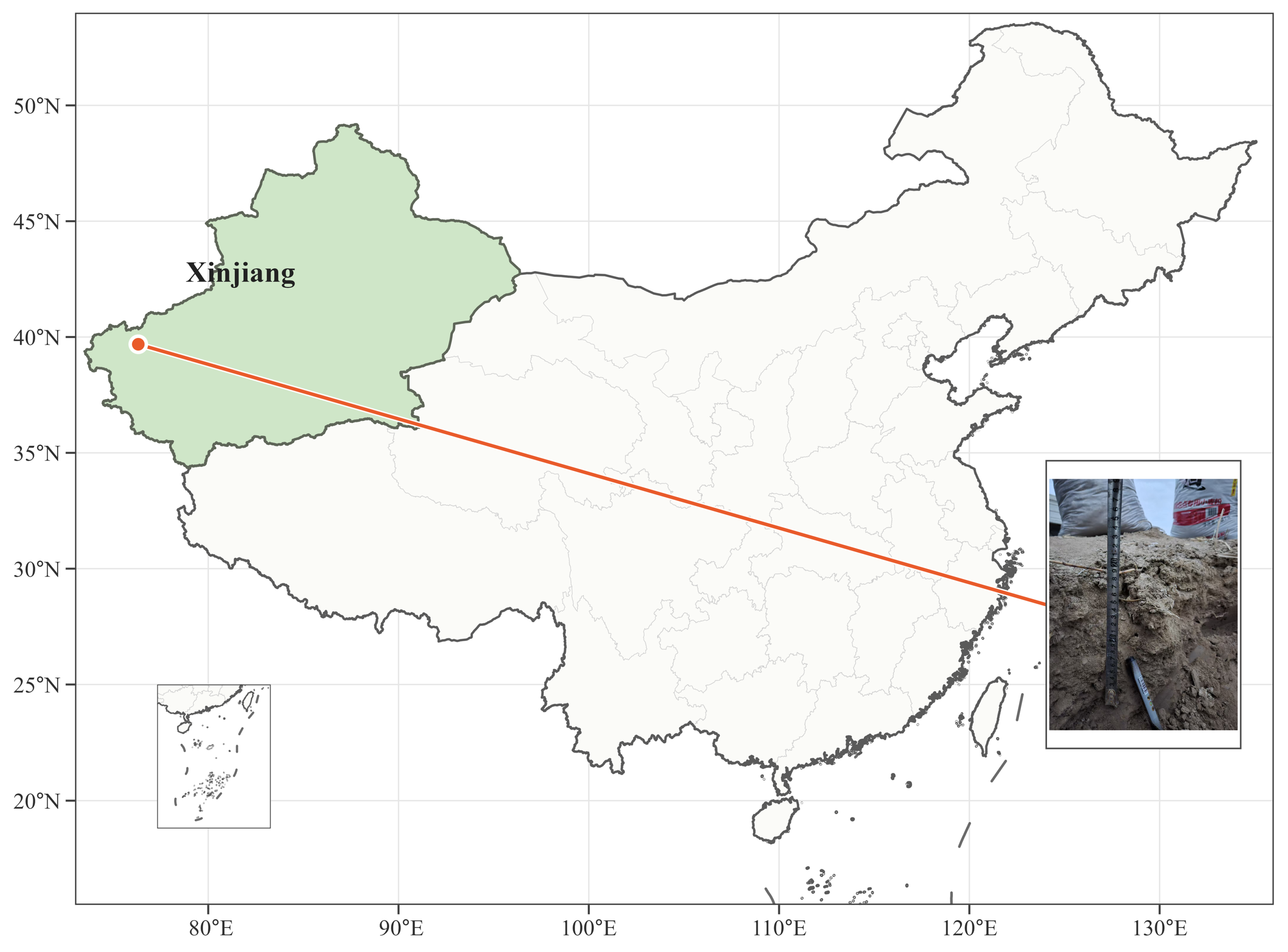
To simulate saline soils in arid regions containing a low-permeability interlayer, soil-box infiltration experiments were conducted in the Key Laboratory of Hydrology and Water Resources at Xinjiang University. The tested soils were collected from saline-alkali land in northeastern Shalatala Village, Gedaliang Township, Artux City, Xinjiang Uyghur Autonomous Region, China (39°41′14″ N, 76°19′25″ E), as shown in Figure 1. Saline soils are widely distributed in the study area, and the soil profile exhibits clear layered differentiation, with alternating layers of different textures. Local fine-particle-enriched or compacted layers readily form weakly permeable interlayers, thereby causing restricted infiltration, interface water stagnation, and surface salt accumulation. Based on field profile observations, samples were collected from the permeable layer and the weakly permeable interlayer of a typical layered saline soil profile. The representativeness of the samples in this study refers to their ability to reflect the typical layered structure observed at the sampling site, rather than statistical representativeness of all saline soils in the region. Therefore, the collected soils were used to support controlled process analysis and model calibration under reconstructed laboratory conditions.

Soil samples were taken from a depth of 40 cm. The filling materials for the soil boxes consisted of a permeable layer (0–20 cm) and a low-permeability layer (>20–40 cm). After transport to the laboratory, both materials were air-dried naturally, cleared of plant residues and roots, crushed, ground, passed through a 1 mm sieve, and thoroughly mixed before use. The 1 mm sieve was used to remove coarse fragments, roots, plant residues, and large aggregates and to reduce random heterogeneity during repacking [44,45,46]. Bulk density was measured by the ring-knife method and was 1.239 g/cm³ for the permeable layer and 1.654 g/cm³ for the low-permeability layer. Particle-size analysis was conducted according to the Standard for Geotechnical Testing Method (GB/T 50123-2019) [47], and the results are listed in

Table 1. Particle-size composition of the tested soils.

Soil Type	Coarse Sand 2–1 (mm)	Coarse Sand 1.0–0.5 (mm)	Medium Sand 0.5–0.25 (mm)	Fine Sand 0.25–0.075 (mm)	Very Fine Sand <0.075 (mm)	Curvature Coefficient Cc	Uniformity Coefficient Cu
Permeable-layer soil	0.0	0.9	4.4	36.2	58.5	0.875	5.200
Low-permeability-layer soil	0.0	0.0	3.8	34.8	61.4	1.504	5.980

. The initial salt content of the permeable-layer soil was 4.04 g/kg, whereas that of the weakly permeable interlayer was 6.65 g/kg. Therefore, the weakly permeable interlayer acted not only as a hydraulic barrier but also as a relatively salt-rich layer in the reconstructed profile. Although both materials were classified as silt according to particle-size distribution, the weakly permeable interlayer was defined based on hydraulic contrast rather than textural class alone. The interlayer soil had a higher bulk density than the permeable-layer soil and was parameterized with lower hydraulic conductivity in the HYDRUS-3D (Program version: 2.05.0250) model. Field profile observations also indicated that this layer acted as a restrictive horizon for downward infiltration. Therefore, the term weakly permeable interlayer refers to its hydraulic role in the layered profile rather than to a distinct textural class.

Six groups of indoor experiments were performed in the Key Laboratory of Hydrology and Water Resources at Xinjiang University. The experimental design is presented in

Table 2. Experimental design.

Experiment ID	Weakly Permeable Interlayer Thickness (cm)	Hole Diameter (cm)	Hole Spacing (cm)
A1	7.5	/	/
A2	15	/	/
A3	22.5	/	/
B1	7.5	5	30
B2	7.5	5	50
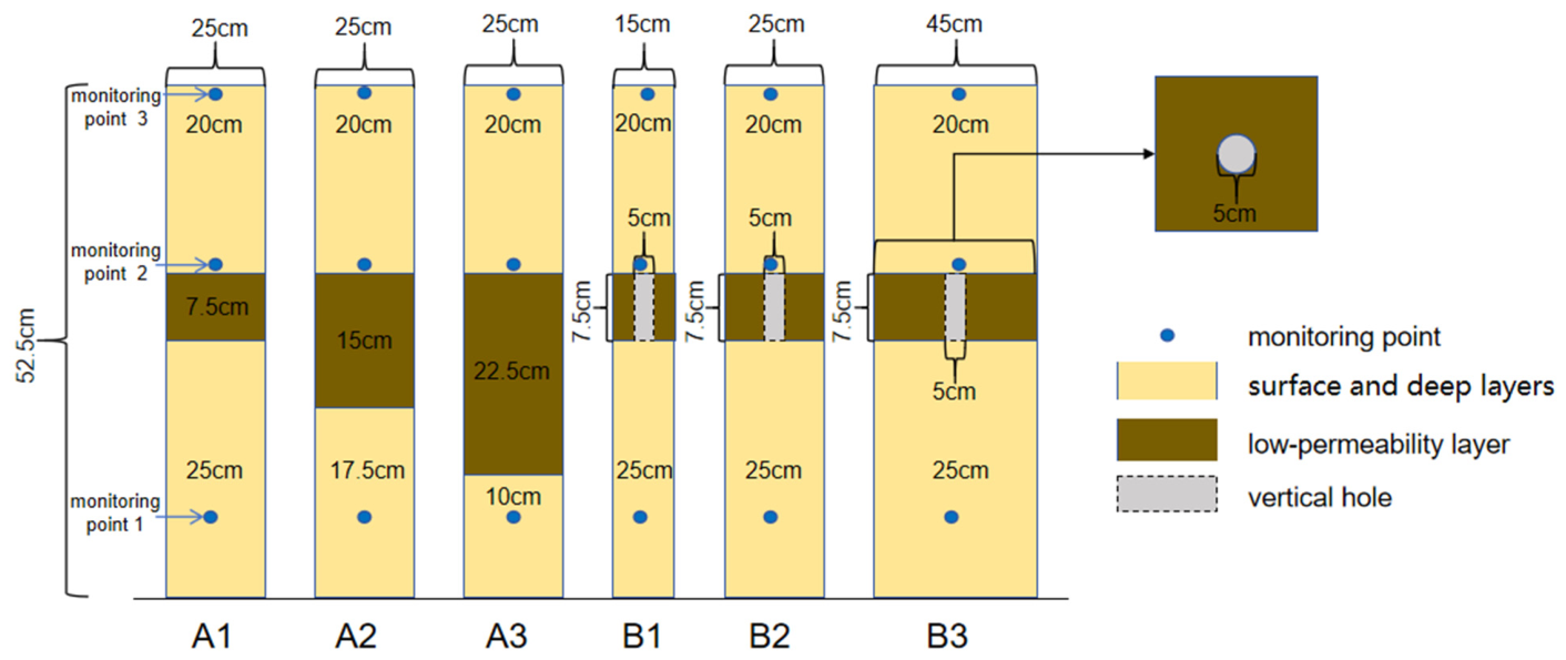
B3	7.5	5	90

. The soil-box experiments were designed as pilot-scale demonstrations for process observation and HYDRUS-3D model calibration/validation rather than as replicated experiments for statistical inference. Each treatment was conducted using one soil box. Therefore, standard deviations, standard errors, and confidence intervals were not calculated from the laboratory data. Quantitative comparisons among extended parameter scenarios were mainly based on the calibrated HYDRUS-3D simulations. Rectangular acrylic soil boxes (Urumqi, China) were used as the outer walls of the seepage apparatus. The experiments were conducted in boxes with length and width dimensions of 15 cm, 25 cm, and 45 cm, and a height of 80 cm. The bottom 5 cm was filled with quartz sand, and a 2 cm filter screen was placed at the interface between the upper 71 cm and the lower quartz-sand layer. A 2 cm base was installed at the bottom, and a valve was placed in the center of the 5 cm quartz-sand layer for venting. Six treatments were designed in total. In three treatments, low-permeability soil layers with thicknesses of 7.5, 15, and 22.5 cm were placed at a burial depth of 20 cm in 25 cm × 25 cm soil boxes and labeled A1, A2, and A3, respectively. In the other three treatments, a 7.5 cm thick low-permeability layer was placed at a burial depth of 20 cm in soil boxes with side lengths of 15, 25, and 45 cm; a cylindrical hole with a diameter of 5 cm was excavated through the center of the low-permeability layer and backfilled with quartz sand. These treatments were labeled B1, B2, and B3. Schematic profiles of the different treatments are shown in Figure 2.

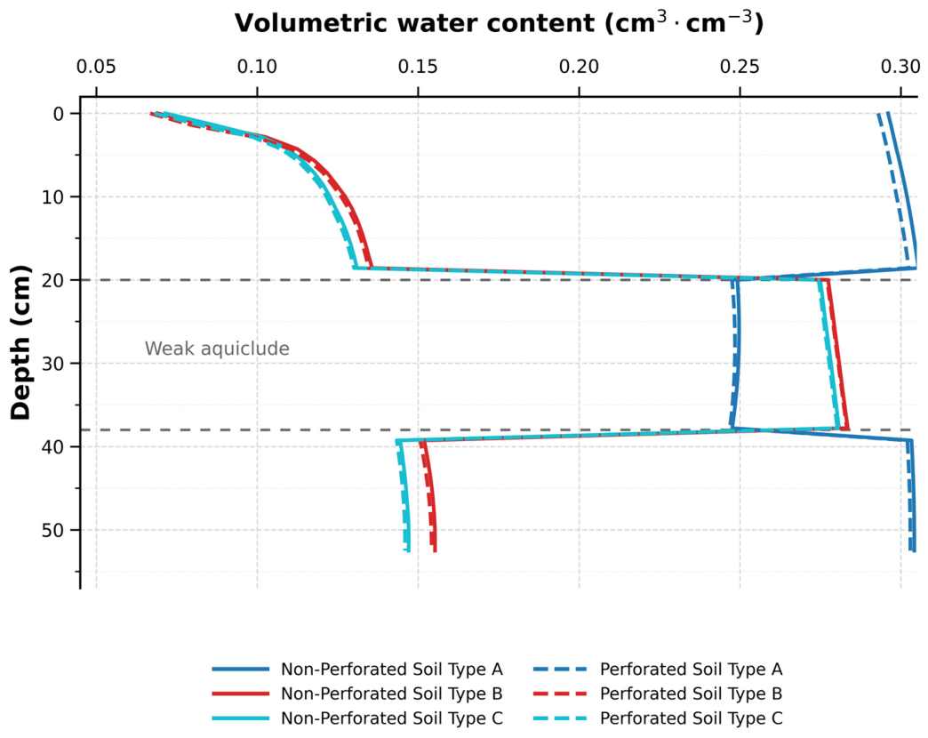
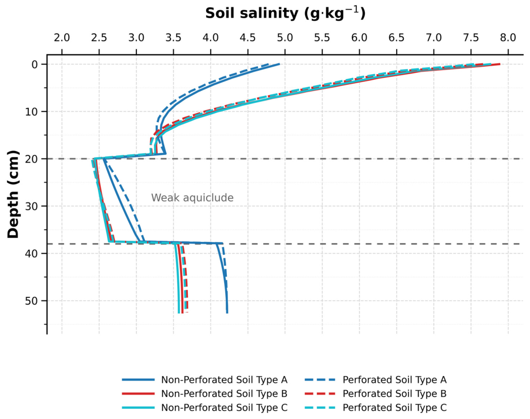
A free space of 18.5 cm was left at the top of each soil box, and the remaining 52.5 cm was filled with soil. The mass of soil corresponding to each 5 cm layer was weighed according to bulk densities of 1.239 g/cm³ and 1.654 g/cm³ for the permeable and low-permeability layers, respectively. The soil was packed layer by layer, with each layer leveled before the next one was added. Soil sensors (MTD15) (Shanghai, China) were installed at depths of 1.0, 19.5, and 45 cm in the center of the soil profile and connected to a data logger (EM50) (Washington, DC, USA) to record temporal changes in volumetric water content and electrical conductivity. The three monitoring depths were selected to represent the surface evaporation-affected layer, the interlayer-interface zone, and the deep drainage-response layer, respectively. These sensors were used mainly to record temporal dynamics for model calibration and validation. They were not intended to provide a high-resolution continuous profile, especially near the upper and lower boundaries of the weakly permeable interlayer, where strong gradients may occur. After the boxes were packed, they were left to equilibrate for 48 h before irrigation. A predesigned volume of water was then applied at the soil surface in a single event. The irrigation water salinity was 3.0 g/L, and the irrigation depth was 120 mm.

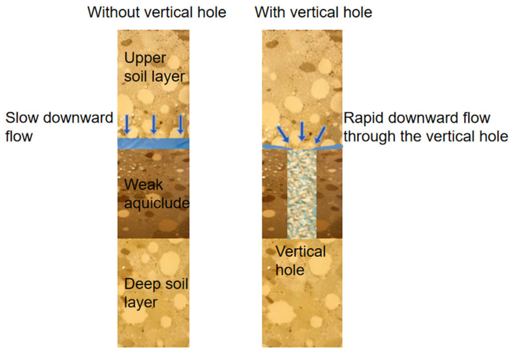
The drainage mechanism of the vertical-hole treatment is illustrated in Figure 3. In heterogeneous layered soils containing a weakly permeable interlayer, infiltrating water in the profile without vertical holes is impeded once it reaches the top boundary of the weakly permeable interlayer, resulting in a pronounced reduction in vertical flux. Water therefore tends to stagnate above the interlayer, which is unfavorable for profile drainage and salt leaching. In contrast, when vertical holes are installed, water that would otherwise be blocked at the interlayer interface converges toward the holes under the hydraulic gradient and rapidly passes through the weakly permeable interlayer via the highly conductive pathway inside the hole. This substantially enhances hydraulic connectivity between the upper and lower layers, promotes deep percolation and downward salt migration, mitigates salt accumulation above the interlayer, and ultimately improves the overall desalinization of layered saline soils.

2.2. Numerical Simulation

Indoor experiments can directly reflect water–salt migration in soils containing a low-permeability layer under vertical-hole treatment, but they are limited by experimental duration, labor intensity, monitoring cost, and the number of feasible scenarios. It is therefore difficult to systematically analyze multifactor combinations involving interlayer thickness, hole diameter, hole spacing, irrigation salinity, and hydraulic-parameter scenarios. To overcome these limitations, a numerical model was developed on the basis of the indoor experiments. After calibration and validation against the pilot-scale observations, the model was used for controlled-condition scenario analysis to compare the relative effects of interlayer thickness, hole geometry, irrigation salinity, and hydraulic-parameter scenario.

HYDRUS-3D was used to simulate the dynamic changes in soil water and salt under different low-permeability interlayer thicknesses and vertical-drainage conditions.

Water flow in the soil was described by the Richards equation [48]:

$${\displaystyle \frac{\partial \mathrm{\theta }}{\partial \mathrm{t}}}={\displaystyle \frac{\partial }{\partial \mathrm{x}}}[\mathrm{K}(\mathrm{\theta }){\displaystyle \frac{\partial \mathrm{\theta }}{\partial \mathrm{x}}}]+{\displaystyle \frac{\partial }{\partial \mathrm{y}}}[\mathrm{K}(\mathrm{\theta }){\displaystyle \frac{\partial \mathrm{\theta }}{\partial \mathrm{y}}}]+{\displaystyle \frac{\partial }{\partial \mathrm{z}}}[\mathrm{K}(\mathrm{\theta }){\displaystyle \frac{\partial \mathrm{\theta }}{\partial \mathrm{z}}}]+{\displaystyle \frac{\partial \mathrm{K}(\mathrm{\theta })}{\partial \mathrm{z}}}-\mathrm{S}$$

(1)

where θ is volumetric water content (cm³/cm³), t is time (d), x is the horizontal coordinate (cm), y is the longitudinal coordinate (cm), z is the vertical coordinate (cm), K(θ) is the unsaturated hydraulic conductivity (cm/d), and S is the soil-surface evaporation term (cm/d).

Solute transport was described by the convection–dispersion equation:

$${\displaystyle \frac{\partial (\mathrm{\theta }\mathrm{c})}{\partial \mathrm{t}}}={\displaystyle \frac{\partial }{\partial \mathrm{x}}}({\mathrm{D}}_{\mathrm{x}}{\displaystyle \frac{\partial \mathrm{c}}{\partial \mathrm{x}}})+{\displaystyle \frac{\partial }{\partial \mathrm{y}}}({\mathrm{D}}_{\mathrm{y}}{\displaystyle \frac{\partial \mathrm{c}}{\partial \mathrm{y}}})+{\displaystyle \frac{\partial }{\partial \mathrm{z}}}({\mathrm{D}}_{\mathrm{z}}{\displaystyle \frac{\partial \mathrm{c}}{\partial \mathrm{z}}})-{\displaystyle \frac{\partial ({\mathrm{q}}_{\mathrm{x}}\mathrm{c})}{\partial \mathrm{x}}}-{\displaystyle \frac{\partial ({\mathrm{q}}_{\mathrm{y}}\mathrm{c})}{\partial \mathrm{y}}}-{\displaystyle \frac{\partial ({\mathrm{q}}_{\mathrm{z}}\mathrm{c})}{\partial \mathrm{z}}}$$

(2)

where θ is volumetric water content (cm³/cm³), c is soil salt concentration (g/cm³), t is time (d), Dx, Dy, and Dz are the hydrodynamic dispersion coefficients (cm²/d), and q is the soil water flux (cm/d). In this study, soil salinity was treated as an apparent conservative total salt variable. This simplification was adopted because the main objective was to compare the effects of weakly permeable interlayers and vertical holes on physical water-flow pathways and total salt redistribution, rather than to resolve ion-specific geochemical reactions. Therefore, the results should be interpreted as total-salinity redistribution rather than multicomponent reactive transport.

The van Genuchten model was used to describe the soil water retention curve [49,50]:

$$\mathrm{\theta }(\mathrm{h})=\left\{\begin{array}{c}{\mathrm{\theta }}_{\mathrm{r}}+{\displaystyle \frac{{\mathrm{\theta }}_{\mathrm{s}}-{\mathrm{\theta }}_{\mathrm{r}}}{[1+{|{\mathrm{\alpha }\mathrm{h}|}^{\mathrm{n}}]}^{\mathrm{m}}}} \mathrm{h}<0\\ {\mathrm{\theta }}_{\mathrm{s}} \mathrm{h}\ge 0\end{array}\right.$$

(3)

$$\mathrm{K}(\mathrm{h})={\mathrm{K}}_{\mathrm{s}}·{\mathrm{S}}_{\mathrm{e}}^{\mathrm{l}}{\left[1-{\left(1-{\mathrm{S}}_{\mathrm{e}}^{{\displaystyle \frac{1}{\mathrm{m}}}}\right)}^{\mathrm{m}}\right]}^2$$

(4)

where θ_s is saturated water content (cm³/cm³), θ_r is residual water content (cm³/cm³), Ks is saturated hydraulic conductivity (cm/d), α (cm⁻¹), n (-), and m (-) are shape parameters of the soil water retention curve, Se is effective saturation (-), and l is the pore-connectivity parameter (-), $\mathrm{m}=1-{\displaystyle \frac{1}{\mathrm{n}}}{;\mathrm{S}}_{\mathrm{e}}={\displaystyle \frac{\mathrm{\theta }-{\mathrm{\theta }}_{\mathrm{r}}}{{\mathrm{\theta }}_{\mathrm{s}}-{\mathrm{\theta }}_{\mathrm{r}}}}$.

According to the soil-box experimental design, the upper boundary was set as an atmospheric boundary to represent irrigation infiltration and post-irrigation evaporation. The irrigation depth was 120 mm, the irrigation intensity was 6 cm/d, and the irrigation duration was 2 d. In the baseline simulation, the potential evaporation rate was set to 0.05 cm/d.

To assess the uncertainty associated with evaporation-boundary representation, an additional evaporation-attenuation scenario was introduced. This scenario was used to approximate the reduction in actual evaporation caused by post-irrigation surface drying, crusting, cracking, or salt crust formation. In this scenario, the evaporation rate was kept at 0.05 cm/d during the early post-irrigation stage and then reduced to 0.035 cm/d and 0.025 cm/d during the later redistribution period. All other parameters and boundary conditions were kept unchanged.

The lower boundary was set as a free-drainage boundary to remain consistent with the laboratory drainage condition. The side boundaries were set as zero-flux boundaries because the acrylic soil boxes were impermeable. These side boundaries help isolate the vertical-hole effect under controlled conditions, but they also restrict lateral redistribution and may enhance the apparent vertical drainage effect compared with field conditions. Therefore, field-scale application requires recalibration under more realistic lateral and groundwater boundary conditions.

To systematically reveal the effects of vertical-hole treatment on water–salt transport in heterogeneous layered soils and to distinguish the individual and coupled roles of interlayer thickness, hole geometry, irrigation salinity, and hydraulic-parameter scenario, 20 simulation scenarios (SA1–SE4) were designed, as listed in

Table 3. Design of simulation scenarios.

Scenario ID	Weakly Permeable Interlayer Thickness (cm)	Hole Diameter (cm)	Hole Spacing (cm)	Irrigation Salinity (g/L)	Hydraulic-Parameter Scenario
SA1	0	/	/	3	A
SA2	7.5	/	/	3	A
SA3	12.5	/	/	3	A
SA4	15	/	/	3	A
SA5	17.5	/	/	3	A
SA6	22.5	/	/	3	A
SB1	17.5	5	50	3	A
SB2	17.5	7.5	50	3	A
SB3	17.5	10	50	3	A
SC1	17.5	5	30	3	A
SC2	17.5	5	70	3	A
SC3	17.5	5	90	3	A
SD1	17.5	/	/	0	A
SD2	17.5	/	/	1.5	A
SD3	17.5	5	50	0	A
SD4	17.5	5	50	1.5	A
SE1	17.5	5	50	3	B
SE2	17.5	5	50	3	C
SE3	17.5	/	/	3	B
SE4	17.5	/	/	3	C

. These scenarios were used to compare the effects of weakly permeable interlayer thickness, hole diameter, hole spacing, irrigation salinity, and hydraulic-parameter scenario.

The SA group represented variations in weakly permeable interlayer thickness and was used to identify the control exerted by the low-permeability layer on soil water–salt redistribution. Under an irrigation salinity of 3 g/L and hydraulic-parameter scenario A, the interlayer thickness was set to 0, 7.5, 12.5, 15, 17.5, and 22.5 cm. SA1 served as the control without a weakly permeable interlayer, whereas the remaining scenarios were used to characterize the effects of different interlayer thicknesses on infiltration, water stagnation, and salt migration.

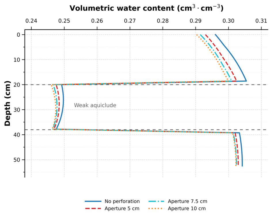
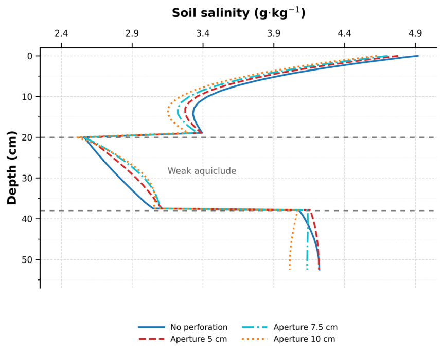
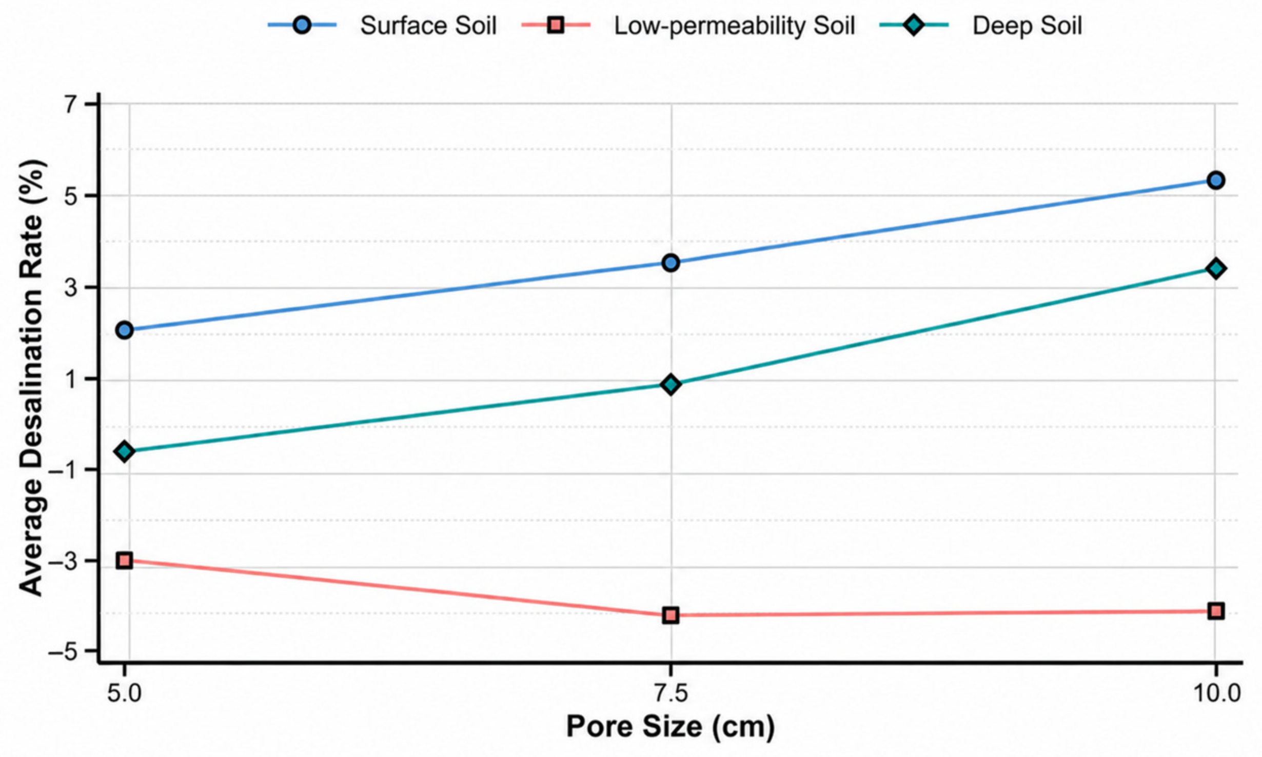
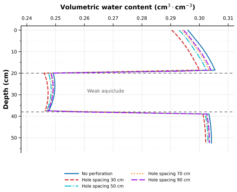
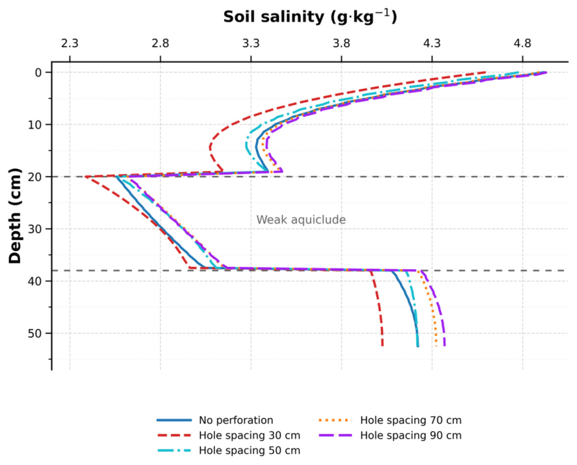
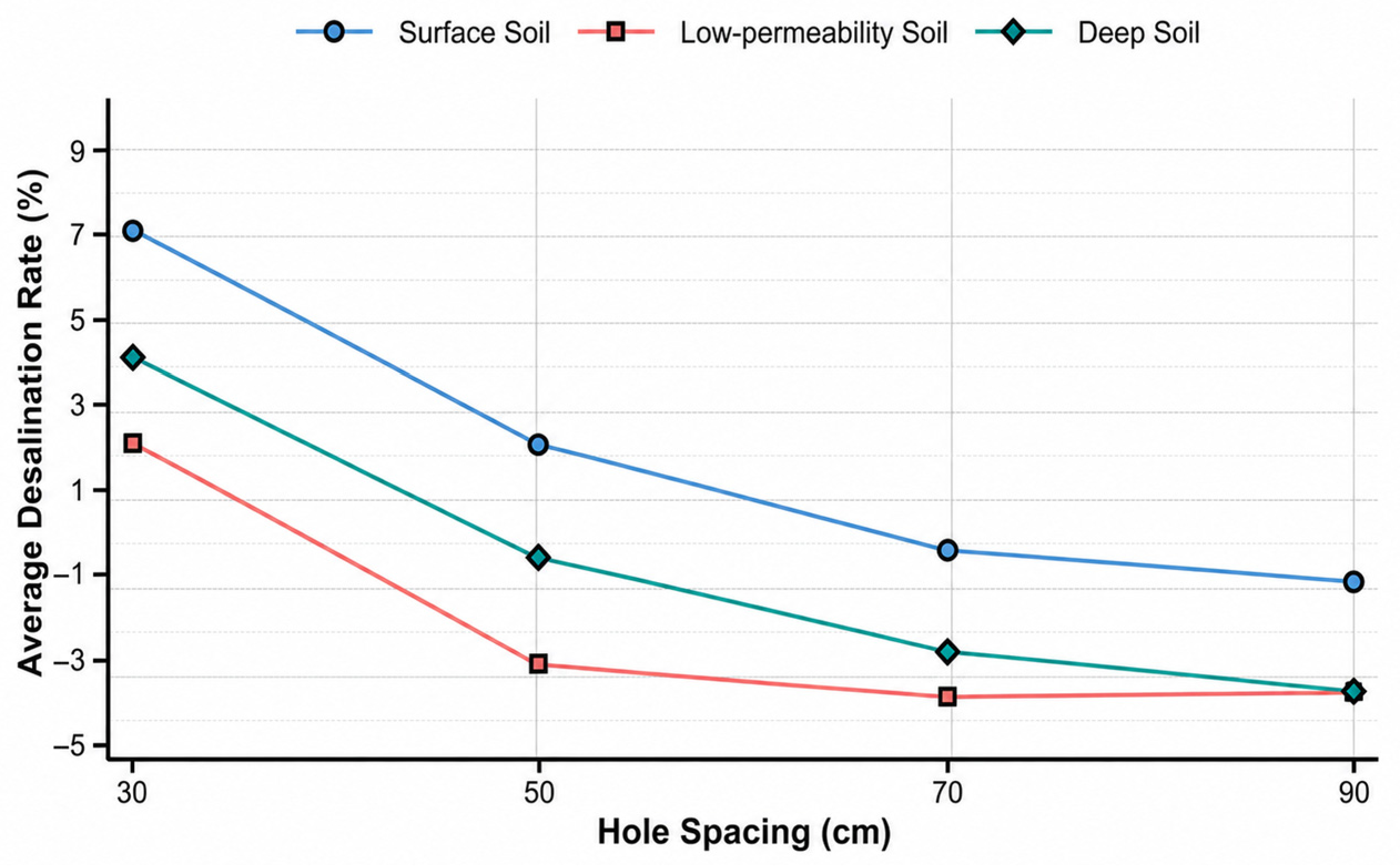
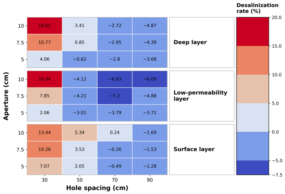
The SB and SC groups represented variations in vertical-hole parameters and were used to analyze the extent to which hole geometry weakened the barrier effect of the weakly permeable interlayer. In both groups, the interlayer thickness was fixed at 17.5 cm, irrigation salinity at 3 g/L, and hydraulic-parameter scenario at A. In group SB, hole spacing was fixed at 50 cm, and hole diameter was set to 5, 7.5, and 10 cm to examine the effect of diameter on preferential flow and salt removal. In group SC, hole diameter was fixed at 5 cm, and hole spacing was set to 30, 70, and 90 cm to compare water–salt transport under different hole densities.

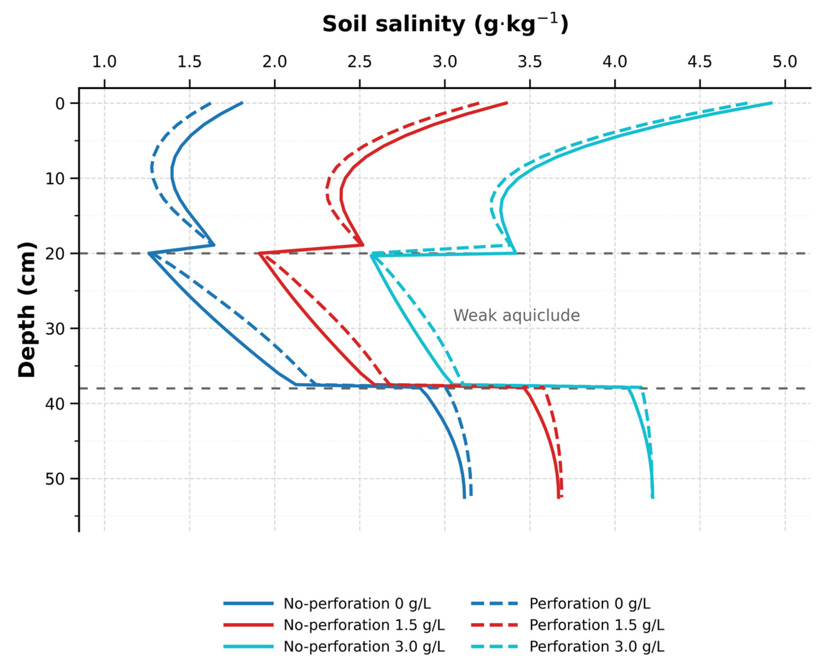
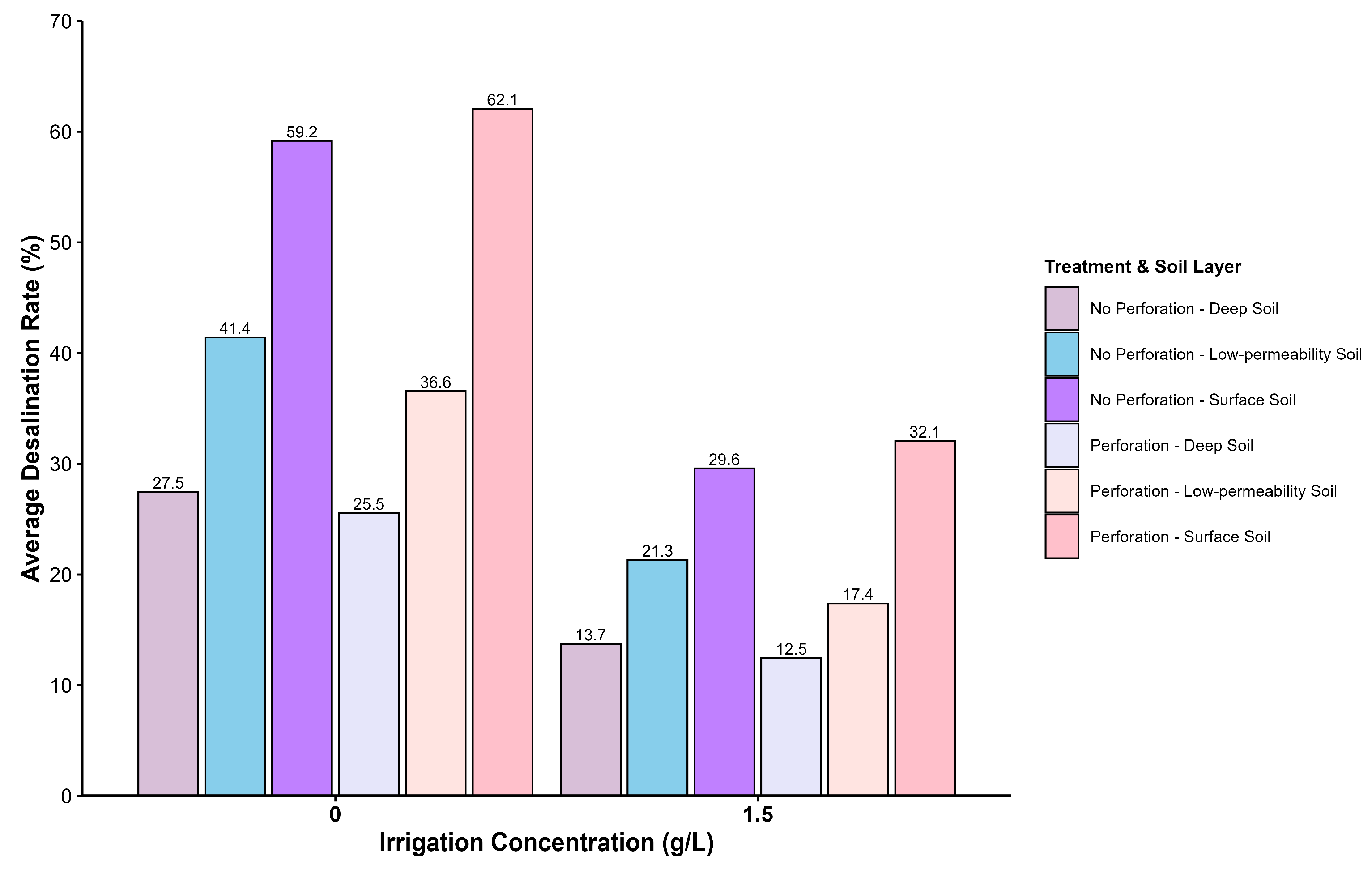
The SD group represented variations in irrigation salinity and was used to analyze how exogenous salt input affected the regulatory effect of the vertical-hole treatment. With an interlayer thickness of 17.5 cm and hydraulic-parameter scenario A, irrigation salinity was set to 0, 1.5, and 3 g/L. SD1 and SD2 were scenarios without vertical holes, whereas SD3 and SD4 included vertical holes (5 cm diameter and 50 cm spacing), allowing comparison of salt leaching and transport pathways under different irrigation salinity levels.

The SE group represented hydraulic-parameter scenarios and was used to explore the sensitivity of water–salt redistribution to permeable-layer hydraulic conductivity. With an interlayer thickness of 17.5 cm and irrigation salinity of 3 g/L, parameter sets B and C were considered. Set B was established using typical empirical hydraulic parameters available in HYDRUS, whereas set C was derived from set B by increasing the saturated hydraulic conductivity of the permeable layer. SE1 and SE2 included vertical holes, whereas SE3 and SE4 were the corresponding no-hole scenarios. These scenarios were used for sensitivity analysis rather than as independently measured soil types.

Overall, this study adopted a one-factor-at-a-time grouping strategy with progressive variation of local parameters. Under otherwise identical conditions, each key factor was examined stepwise so as to provide a controlled-condition basis for comparing the relative effects of key factors and for preliminary layout screening.

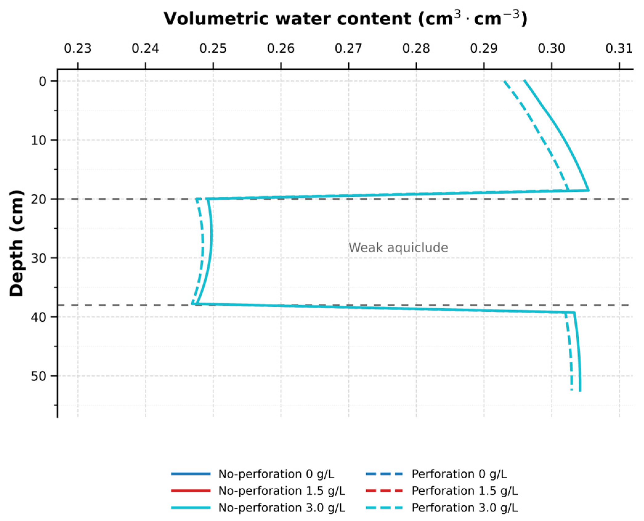
To quantify the local conductive effect of vertical holes, velocity and water-content cross-sections were extracted from HYDRUS-3D at the lower boundary of the weakly permeable interlayer, i.e., at a depth of 37.5 cm, at day 20. The cross-section was divided into the sand-filled hole region and the surrounding matrix region according to the geometric hole diameter. The hole-to-matrix velocity ratio was calculated using the mean velocity in the two regions. In addition, the line-integrated velocity contribution of the hole region was calculated as:

$$R_{\mathrm{v}}={\displaystyle \frac{{\int }_{{\mathrm{\Omega }}_{\mathrm{h}}}{\mathrm{v}}_{\mathrm{z}}\left(\mathrm{x}\right)\hspace{0.17em}\mathrm{d}\mathrm{x}}{{\int }_{{\mathrm{\Omega }}_{\mathrm{t}}}{\mathrm{v}}_{\mathrm{z}}\left(\mathrm{x}\right)\hspace{0.17em}\mathrm{d}\mathrm{x}}}$$

(5)

where Ω_h denotes the sand-filled hole region, Ω_t denotes the entire horizontal cross-section, and v_z(x) is the vertical water velocity at position x.

A water-content-weighted velocity contribution was further calculated as:

$$R_{\mathrm{\theta }\mathrm{v}}={\displaystyle \frac{{\int }_{{\mathrm{\Omega }}_{\mathrm{h}}}{\mathrm{\theta }(\mathrm{x})\mathrm{v}}_{\mathrm{z}}\left(\mathrm{x}\right)\hspace{0.17em}\mathrm{d}\mathrm{x}}{{\int }_{{\mathrm{\Omega }}_{\mathrm{t}}}{\mathrm{\theta }(\mathrm{x})\mathrm{v}}_{\mathrm{z}}\left(\mathrm{x}\right)\hspace{0.17em}\mathrm{d}\mathrm{x}}}$$

(6)

where θ(x) is the volumetric water content. This indicator was used to approximate the relative contribution of the hole region to water transmission across the weakly permeable interlayer.

2.3. Simulation-Derived Empirical Drainage–Desalination Relationship for Preliminary Layout Screening

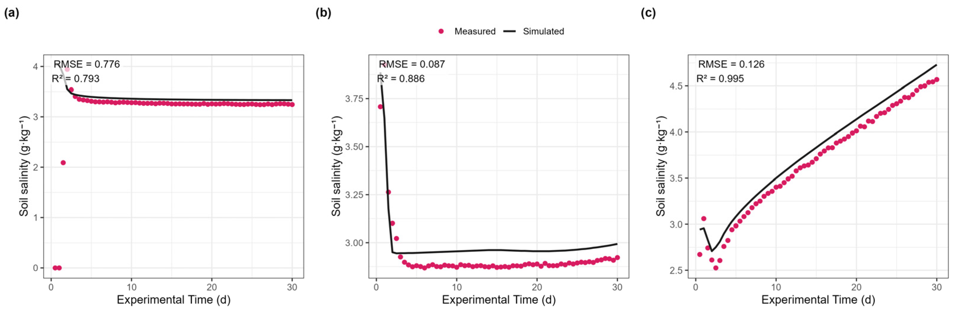
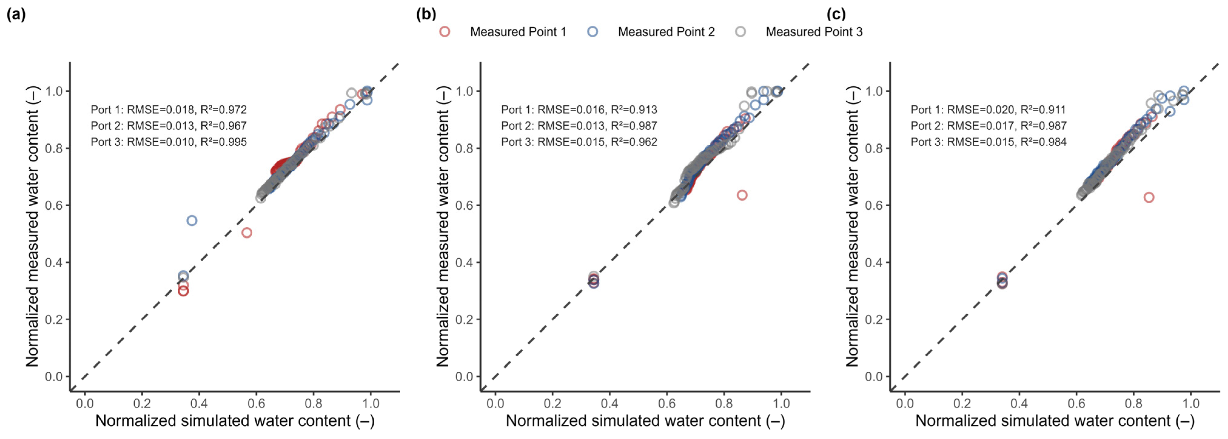
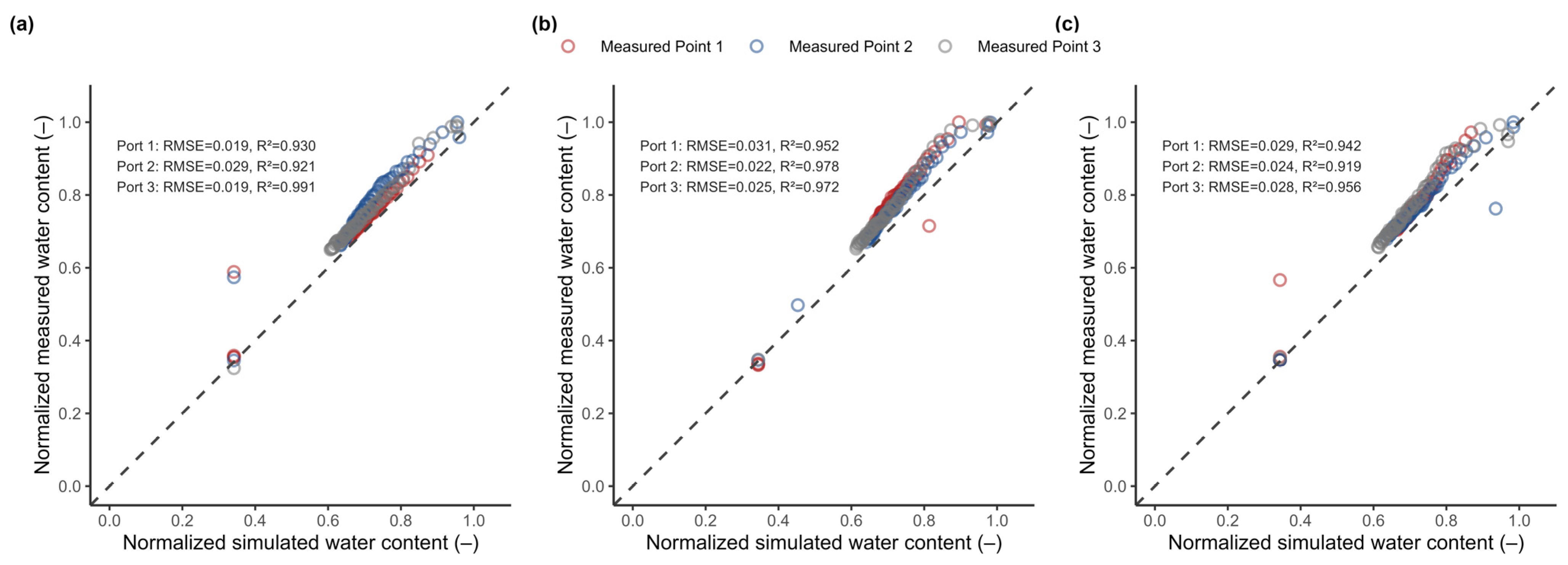
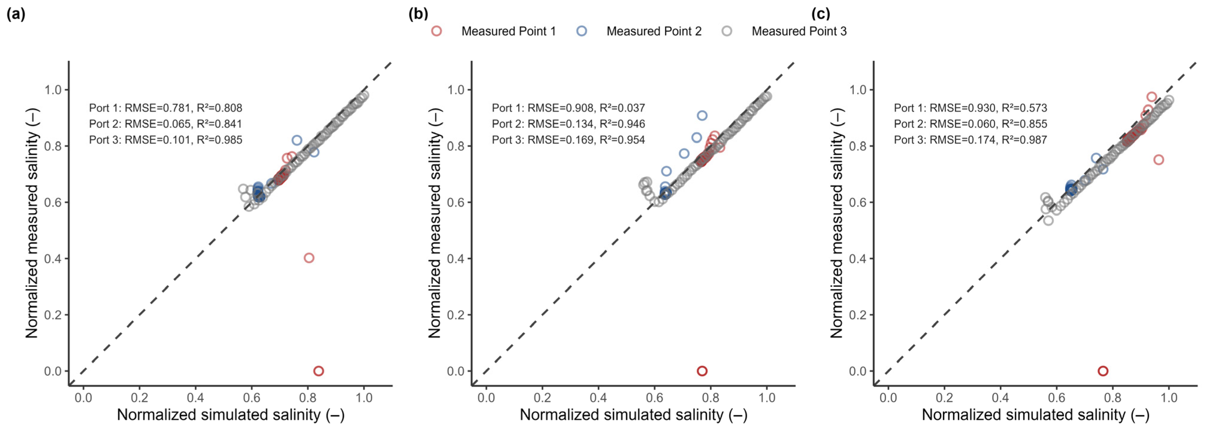
On the basis of the above indoor experiments and numerical simulations, the model was shown to adequately reproduce water–salt transport in soils containing a low-permeability layer under different conditions. The simulations not only provided profile distributions of water and salt under different interlayer thicknesses, hole diameters, hole spacings, irrigation salinities, and hydraulic-parameter scenarios but also allowed extraction of salt-removal indicators for systematic comparison of desalinization performance among parameter combinations. Based on the calibrated HYDRUS-3D simulations, a simulation-derived empirical relationship was established to summarize the combined effects of hole diameter and hole spacing on short-term desalination response. This relationship was intended for preliminary comparison of vertical-hole layouts under the controlled profile structure and boundary conditions considered in this study. It should not be interpreted as an independently validated engineering design model.

To compare the effects of vertical-hole layout parameters under the controlled conditions considered in this study, an empirical relationship was established based on the soil desalination rate. This model was designed to describe the combined regulation of profile desalinization by hole diameter and hole spacing and to provide a methodological basis for subsequent empirical fitting and identification of critical hole spacing.

The desalinization rate was selected as the basic evaluation index. It was defined as the percentage reduction in soil salt content relative to a reference treatment and was used to characterize the extent to which the vertical-hole treatment reduced soil salinity. Because this study focused on the improvement achieved by the vertical-hole treatment relative to the no-hole condition, the mean soil salt content under the treatment with a low-permeability layer thickness of 17.5 cm and without holes was taken as the reference. The desalinization rate was calculated as follows:

$$\mathrm{\eta }={\displaystyle \frac{{\mathrm{S}}_1-{\mathrm{S}}_2}{{\mathrm{S}}_1}}$$

(7)

where η is the soil desalinization rate (%), S₁ is the mean soil salt content (g/kg) under the reference treatment with a 17.5 cm low-permeability layer and no holes, and S₂ is the mean soil salt content (g/kg) in the corresponding layer under the vertical-hole treatment. A larger η indicates a better salt-removal effect, whereas η < 0 indicates salt accumulation relative to the reference treatment.

All indoor experiments lasted 30 d and consisted of an irrigation stage followed by an evolution stage dominated by water redistribution, evaporative consumption, and salt migration. Because water–salt transport during the early stage was strongly controlled by irrigation input and inter-treatment differences had not yet fully developed, whereas the late stage could be affected by boundary effects and end-state convergence, day 20 was selected as the representative analysis time for the simulation scenarios. This time point falls in the middle-to-late period after irrigation, when the effects of weakly permeable interlayer blockage, hole-induced drainage, and evaporative concentration are all well expressed, and differences among treatments in profile water–salt distribution and desalinization become clear. Day 20 was used only as a representative analysis time within the 30 d transient post-irrigation redistribution period. It should not be interpreted as a steady-state, seasonal, or long-term engineering evaluation time. Therefore, all day-20 desalination indicators and empirical relationships represent short-term responses under a single-irrigation event and controlled laboratory boundary conditions.

To summarize the short-term desalination response under different hole diameters and spacings, an empirical expression was further established based on the simulation results. for different hole diameters and spacings. Because the primary management goals in irrigation districts are to reduce salt stress in the crop root zone and to promote downward migration and discharge of salts for long-term desalinization, the surface and deep layers were selected as the two key evaluation layers. The surface-layer desalinization rate was used to characterize improvement in the root-zone salt environment, whereas the deep-layer desalinization rate was used to characterize whether salts were continuously displaced downward and discharged from the profile. The low-permeability layer mainly reflects interlayer blockage and transient salt retention and was therefore not used as a core engineering evaluation item in this section. To obtain a composite indicator that accounts for both root-zone improvement and long-term desalinization, the root zone-deep layer mean desalinization rate was defined as:

$${\mathrm{\eta }}_{20}^{(\mathrm{R}-\mathrm{D})}={\displaystyle \frac{{\mathrm{\eta }}_{\mathrm{s}\mathrm{u}\mathrm{r}\mathrm{f}\mathrm{a}\mathrm{c}\mathrm{e},20}+{\mathrm{\eta }}_{\mathrm{d}\mathrm{e}\mathrm{e}\mathrm{p},20}}{2}}$$

(8)

where ${\mathrm{\eta }}_{20}^{(\mathrm{R}-\mathrm{D})}$ is the root zone-deep layer mean desalinization rate on day 20 (%), and η_surface,20 and η_deep,20 are the desalinization rates (%) of the surface and deep layers on day 20, respectively. A larger value indicates that the vertical-hole treatment is more favorable for improving the root-zone salt environment and promoting downward salt migration and discharge.

Simulation results for different diameter–spacing combinations presented in later sections show that this composite index decreases with increasing hole spacing and increases with increasing hole diameter, with a clear interaction between the two variables. Because hole density can be represented by 1/S, the following empirical form was selected to describe the relationship between the day-20 root zone-deep layer mean desalinization rate and hole diameter and spacing while maintaining both physical interpretability and model simplicity:

$${\mathrm{\eta }}_{20}^{(\mathrm{R}-\mathrm{D})}={\mathrm{\beta }}_0+{\mathrm{\beta }}_1\mathrm{D}+{\displaystyle \frac{{\mathrm{\beta }}_2+{\mathrm{\beta }}_3\mathrm{D}}{\mathrm{S}}}$$

(9)

where D is hole diameter (cm), S is hole spacing (cm), and β₀, β₁, β₂, and β₃ are fitted parameters. The term β₁D represents the direct effect of hole diameter on desalinization, β₂/S represents the contribution of hole density, and β₃D/S characterizes the coupling between hole diameter and hole density. Model parameters were estimated by least squares using simulation results obtained under a low-permeability interlayer thickness of 17.5 cm for multiple combinations of hole diameter and hole spacing.

To identify the threshold at which the system shifts from net desalinization to net salt accumulation under different hole diameters, the root zone-deep layer mean desalinization rate was set equal to zero, yielding the critical hole-spacing function S*(D). When actual hole spacing is smaller than this critical value, the system tends to exhibit net desalinization; when spacing exceeds the critical value, there is a risk of net salt accumulation. This criterion can be used for preliminary comparison of vertical-hole layouts and for determining reasonable hole spacing under different hole diameters.

The empirical drainage–desalination model developed in this study is intended for preliminary comparison of vertical-hole layout parameters under controlled boundary conditions. The model was established on the basis of the initial conditions and profile structure defined here and is therefore applicable within the diameter and spacing ranges investigated in this study. If the profile structure, interlayer thickness, soil hydraulic parameters, evaporation intensity, or irrigation salinity change substantially, the model parameters should be recalibrated while retaining the same functional form in order to improve applicability and extrapolation reliability in other engineering contexts.

3. Results

3.1. Temporal Evolution Characteristics of Water and Salt Transport

To illustrate the typical temporal water–salt response used for model calibration, the pilot-scale soil-box experiment with a hole spacing of 50 cm, a hole diameter of 5 cm, and a weakly permeable interlayer thickness of 7.5 cm was selected as a representative case. Because the laboratory treatments were not replicated, the experimental curves were used to characterize representative process dynamics and to support HYDRUS-3D calibration and validation, rather than to conduct statistical treatment comparisons. Investigation of this typical case helps reveal the basic features of water–salt migration under vertical-hole regulation and provides an experimental basis for subsequent model validation.

3.1.1. Temporal Variation in Soil Water Content

Figure 4 shows the temporal variation in soil water content at different monitoring depths under a hole spacing of 50 cm, a hole diameter of 5 cm, and an interlayer thickness of 7.5 cm. Panels a–c correspond to monitoring depths of 45, 19.5, and 1 cm, respectively. In general, water content increased rapidly after infiltration and then gradually declined and stabilized with time, reflecting progressive drying caused by gravitational drainage and evaporation after infiltration recharge. Overall, the simulated curves were slightly lower than the measured values, indicating a slight underestimation of water content. At 45 cm depth (Figure 4a), the change in water content was relatively small and decreased slowly after the infiltration peak, indicating that evaporative effects were weak at this depth. The model captured the overall trend but showed some deviation in decay rate and stable water-content level. At 19.5 cm depth (Figure 4b), the soil was located in a transition zone where evaporation began to exert influence. Water content at this depth was controlled simultaneously by upward evaporative demand and downward drainage, so minor errors in the evaporation boundary or soil water retention parameters could lead to underestimation during the intermediate stage or overly rapid decay. At 1 cm depth (Figure 4c), evaporation exerted the strongest control, and water content declined most markedly after the peak. Measured values were generally higher than simulated values because actual evaporation decreases as the soil surface dries or crusts, whereas the evaporation boundary in the model did not fully account for surface resistance, causing stronger simulated surface drying and therefore lower water content.

3.1.2. Temporal Variation in Soil Salt Concentration

Figure 5 shows the temporal variation in soil salt content at different monitoring depths under the same experimental conditions. In general, salt content differed among depths, with the deep layer remaining largely stable, the middle layer showing rapid leaching-induced decline, and the surface layer exhibiting continuous accumulation. This pattern reflects the coupled effects of infiltration-driven leaching and evaporation-induced surface salt enrichment. At 45 cm depth (Figure 5a), the deep-layer salt curve was generally stable with only small fluctuations, indicating that upward concentration driven by evaporation scarcely affected the deep layer. At a few early time points, some discrepancy existed between simulated and measured values. The deep-layer salt data showed lower R² and higher RMSE than the other monitoring points because the sensor could not detect soil salinity reliably when water content was very low, and no flow reached the probe; once water flowed into the soil, the sensor functioned normally, and later data were unaffected. This does not alter the conclusion that the deep layer responded weakly and remained overall stable. At 19.5 cm depth (Figure 5b), salt content declined rapidly at the beginning, indicating dominance of convective leaching, and then remained low with a slight late-stage rebound caused by weak return flux associated with evaporation-driven capillary supply and diffusion–dispersion. The overall fit was good. At 1 cm depth (Figure 5c), salt content first decreased briefly as water infiltrated and then rose continuously after infiltration, reflecting evaporation concentration and surface enrichment. The high R² indicates that the model reproduced the trend of surface salt accumulation well, although the simulated values were slightly higher than the observed values in the middle and late stages because surface processes such as evaporation attenuation, salt crusting, and salt precipitation were not fully represented.

3.2. Model Validation

Comparison Between Simulated and Experimental Results

Figure 6a–c compares measured and simulated soil water content under weakly permeable interlayer thicknesses of 7.5, 15, and 22.5 cm, respectively, and also presents scatter plots of normalized water content for the three treatments. In all cases, the scatter points were concentrated near the 1:1 line, indicating that the HYDRUS model reliably reproduced the magnitude and variation range of temporal water-content dynamics in layered heterogeneous soils and exhibited good transferability. With respect to monitoring depth, the scatter for Port1 (45 cm) and Port2 (19.5 cm) was more concentrated, suggesting that water processes dominated by gravitational drainage and interlayer redistribution in the middle and deep profile were more readily captured by equivalent parameters. By contrast, Port3 (1 cm) showed slight dispersion in the high-water-content range, indicating greater sensitivity of the surface layer to actual evaporation attenuation, surface resistance (e.g., crusting or cracking), and local preferential flow when an evaporation boundary is present. As the weakly permeable interlayer became thicker, local dispersion increased slightly, implying that stronger blockage made interlayer water retention and redistribution more complex, although overall model performance remained high.

Figure 7a–c shows the comparison between measured and simulated soil water content for hole spacings of 30, 50, and 90 cm, respectively, together with scatter plots of normalized water content. Under all three spacings, the scatter points were distributed mainly along the 1:1 line, indicating that the model adequately represented the effect of vertical-hole layout on soil water status. With increasing hole spacing, the dispersion of the scatter points increased slightly, especially at the surface Port3 (1 cm). This suggests that larger spacing created greater heterogeneity in infiltration recharge, so the surface layer exhibited greater local differences during repeated infiltration-evaporation cycles, such as co-occurrence of preferential infiltration near holes and insufficient recharge in non-hole zones, thereby increasing deviation of observations from simulations. Even so, the overall trends were consistent, indicating that the model is suitable for different hole-spacing conditions.

Figure 8a–c compares measured and simulated soil salt content for weakly permeable interlayer thicknesses of 7.5, 15, and 22.5 cm, respectively, and presents scatter plots of normalized salt content for the three treatments. Overall, most points were close to the 1:1 line, indicating that the model captured convective-dispersive salt transport associated with water movement and reproduced the overall intensity of salt leaching and redistribution observed in the experiments. Compared with water content, however, salt content scatter plots showed a few more outliers, and these deviations tended to occur in specific stages or ranges. On the one hand, the surface layer (Port3) was characterized by salt enrichment and steep concentration gradients under evaporation, making salt dynamics more sensitive to the evaporation boundary, dispersion parameters, and surface processes such as salt precipitation or crusting that affect effective evaporation. On the other hand, outliers in the deep layer Port1 (45 cm) were more likely under low-salt or abrupt-transition conditions because salt variation there was small, sensor noise became more important, and local heterogeneity produced short-term fluctuations in solute flux. Despite these few outliers, the overall fit indicates that the model is suitable for simulating salt transport under different weakly permeable interlayer thicknesses.

Figure 9a–c shows the comparison between measured and simulated soil salt content for hole spacings of 30, 50, and 90 cm, respectively, together with scatter plots of normalized salt content. Overall, the points still lie mainly along the 1:1 line, demonstrating that the model captured the effect of hole spacing on salt migration and leaching efficiency. As spacing increased, the degree of scatter also increased slightly, and the surface Port3 (1 cm) was particularly sensitive, indicating that larger spacing weakened the spatial uniformity of local leaching and made evaporation-driven surface salt accumulation more spatially heterogeneous (i.e., different between zones near holes and zones away from holes). Meanwhile, Port2 (19.5 cm) remained closely distributed around the 1:1 line, suggesting that salt processes in the middle layer were still controlled mainly by infiltration and redistribution. These results support use of the model for subsequent analysis across a broader parameter space.

Overall, the model reproduced the main temporal patterns of soil water redistribution and salt transport under the tested interlayer thickness and hole-spacing conditions. However, model performance was stronger for soil water content than for soil salinity. Salt simulations showed larger scatter, especially in the deep layer and during early low-water-content periods, when sensor-based salinity readings were less stable. Therefore, the subsequent simulations should be interpreted as controlled-condition scenario analysis rather than independently validated field-scale predictions.

To provide a clearer overview of model performance, the main validation metrics were further summarized by variable and monitoring depth (

Table 4. Summary of HYDRUS-3D model performance for soil water content and soil salinity at different monitoring depths.

Variable	Monitoring Depth	Time-Series Validation RMSE	Time-Series Validation R2	Normalized Validation RMSE Range	Normalized Validation R2 Range	Main Interpretation
Soil water content	45 cm	0.031	0.952	0.016–0.031	0.911–0.972	The model reproduced deep-layer water dynamics well, although slight deviations occurred during post-irrigation drainage.
Soil water content	19.5 cm	0.022	0.978	0.013–0.029	0.919–0.987	The model showed good agreement at the interlayer-interface zone, indicating reliable simulation of water redistribution near the weakly permeable layer.
Soil water content	1 cm	0.025	0.972	0.010–0.028	0.956–0.995	The model captured the surface water-content trend, but surface results were more sensitive to evaporation-boundary assumptions.
Soil salinity	45 cm	0.776	0.793	0.776–0.945	0.037–0.837	Deep-layer salinity showed the largest uncertainty, mainly due to early-stage sensor instability under very low water-content conditions.
Soil salinity	19.5 cm	0.087	0.886	0.060–0.134	0.841–0.946	The model captured salt leaching and redistribution near the interlayer with generally acceptable accuracy.
Soil salinity	1 cm	0.126	0.995	0.101–0.174	0.954–0.996	The model reproduced the surface salt-accumulation trend well, although the magnitude was sensitive to evaporation and surface resistance processes.

). This table combines the time-series validation metrics from Figure 4 and Figure 5, and the normalized validation ranges from Figure 6, Figure 7, Figure 8 and Figure 9, allowing direct comparison between water-content and salinity simulations.

The summary confirms that HYDRUS-3D reproduced soil water content more reliably than soil salinity. The water-content simulations showed consistently high agreement across depths, whereas salinity simulations exhibited greater uncertainty. In particular, the deep-layer salinity showed larger deviation because early-stage low water content reduced the stability of sensor-based salinity measurements. Therefore, salt transport predictions, especially in the deep layer and in extended unvalidated scenarios, should be interpreted more cautiously than water-content predictions.

To assess the influence of evaporation-boundary uncertainty, representative treatments were compared under the evaporation-attenuation scenario at day 20 (

Table 5. Comparison of representative treatments under the evaporation-attenuation scenario at day 20.

Treatment	Surface Water Content	Surface Salinity (g/kg)	Interlayer Water Content	Interlayer Salinity (g/kg)	Deep-Layer Water Content	Deep-Layer Salinity (g/kg)
No hole	0.3068	3.533	0.2518	2.776	0.3031	4.163
5 cm hole	0.3040	3.466	0.2506	2.855	0.3020	4.189
10 cm hole	0.3014	3.352	0.2495	2.885	0.3013	4.027

). This scenario was used to approximate the reduction in actual evaporation caused by post-irrigation surface drying, crusting, cracking, or salt crust formation.

Under the evaporation-attenuation scenario, the vertical-hole treatments still reduced surface salinity compared with the no-hole treatment. Surface salinity decreased from 3.533 g/kg in the no-hole treatment to 3.466 and 3.352 g/kg in the 5 and 10 cm hole treatments, corresponding to reductions of 1.90% and 5.12%, respectively. The 10 cm hole also reduced deep-layer salinity from 4.163 to 4.027 g/kg, whereas the 5 cm hole slightly increased deep-layer salinity. These results indicate that the evaporation-boundary assumption affected the magnitude of surface water–salt responses but did not reverse the main qualitative trend of vertical-hole treatment.

3.3. Factors Affecting Water and Salt Transport

3.3.1. Effect of Weakly Permeable Interlayer Thickness on Water and Salt Transport

Figure 10 shows the soil-profile water distribution under different weakly permeable interlayer thicknesses. Overall, increasing the thickness of the weakly permeable interlayer increased water retention in the upper profile and reduced downward redistribution. In the profile without a weakly permeable interlayer, the mean surface water content was 0.292 cm³/cm³. When the interlayer thickness increased to 22.5 cm, the mean surface water content increased to 0.304 cm³/cm³. This indicates that a thicker weakly permeable interlayer enhanced water storage above the interlayer. The deep layer showed an opposite water-content response. With increasing interlayer thickness, downward water movement was increasingly restricted, and the mean deep-layer water content decreased. The difference between the surface and deep layers became more evident when the weakly permeable interlayer was thicker, indicating that the interlayer changed the vertical redistribution pattern of water after irrigation. Additional layer-specific salinity results under different weakly permeable interlayer thicknesses are provided in Table S1.

Figure 11 shows the soil-profile salinity distribution under different weakly permeable interlayer thicknesses. Salinity redistribution varied clearly with interlayer thickness. As summarized in Figure 12, the mean surface salinity increased from 3.37 g/kg in the profile without a weakly permeable interlayer to 3.76 g/kg when the interlayer thickness increased to 22.5 cm. This shows that a thicker weakly permeable interlayer increased surface salt accumulation after irrigation. The increase in deep-layer salinity was more pronounced. The mean deep-layer salinity increased from 3.17 to 4.44 g/kg as the weakly permeable interlayer became thicker. In particular, the salinity increase became more evident when the interlayer thickness exceeded approximately 15 cm. Because this pattern was obtained from the tested simulation levels rather than from repeated simulations or formal change-point analysis, 15 cm should be interpreted only as a suggested transition point within the present parameter range, not as a statistically validated threshold.

The increase in deep-layer salinity should be considered together with the initial salinity of different soil layers. In this study, the initial salinity of the surface and deep soils was 4.04 g/kg, whereas that of the weakly permeable interlayer was 6.65 g/kg. Therefore, the weakly permeable interlayer acted not only as a hydraulic restrictive layer but also as a relatively salt-rich layer. As the interlayer became thicker, the amount of salt stored in this layer increased, and part of this salt could be redistributed downward during infiltration and retained in the deep layer under limited drainage.

Overall, increasing weakly permeable interlayer thickness increased surface water retention, enhanced surface salt accumulation, and promoted deep-layer salt retention. These results indicate that the interlayer thickness controlled water–salt redistribution mainly by changing the vertical hydraulic connection and the amount of salt stored within the weakly permeable layer.

3.3.2. Effect of Hydraulic-Parameter Scenario on Water and Salt Transport

The hydraulic parameters in

Table 6. Hydraulic-parameter scenarios.

Hydraulic-Parameter Scenario	Soil Parameter	Permeable Layer	Low-Permeability Layer	Replacement Soil
A	Qr	0.141	0.131	0.051
A	Qs	0.43	0.315	0.394
A	Alpha (1/cm)	0.02	0.016	0.034
A	n	1.41	1.37	1.72
A	Ks (cm/day)	30.8	3	126
A	l	0.5	0.5	0.5
B	Qr	0.065	0.1314	0.045
B	Qs	0.41	0.3147	0.43
B	Alpha (1/cm)	0.075	0.016	0.145
B	n	1.89	1.37	2.68
B	Ks (cm/day)	106.1	3	712.8
B	l	0.5	0.5	0.5
C	Qr	0.065	0.131	0.045
C	Qs	0.41	0.315	0.43
C	Alpha (1/cm)	0.075	0.016	0.145
C	n	1.89	1.37	2.68
C	Ks (cm/day)	156.1	3	712.8
C	l	0.5	0.5	0.5

are van Genuchten–Mualem parameters used in HYDRUS-3D. Parameter set A represents the reconstructed soil system used in the pilot-scale soil-box experiments. It was constrained by measured particle-size distribution and bulk density and further calibrated using observed water-content and salinity dynamics. Parameter sets B and C were not independently measured soil types. Set B was established using typical empirical hydraulic parameters available in HYDRUS, whereas set C was derived from set B by changing the saturated hydraulic conductivity of the permeable layer. Therefore, B and C should be interpreted as scenario-based hydraulic-parameter sets rather than independent soil structural types. In these scenarios, the weakly permeable interlayer thickness was fixed at 17.5 cm. Parameter settings for hydraulic-parameter scenarios A, B, and C are given in Table 6. Additional water-content and salinity results under different hydraulic-parameter scenarios are provided in Table S2.

Figure 13 shows the soil-profile water distribution under different hydraulic-parameter scenarios. Clear differences in water distribution were observed among scenarios A, B, and C. In the surface soil above the weakly permeable interlayer, the mean water contents under the no-hole treatment were 0.301, 0.120, and 0.117 cm³/cm³ for scenarios A, B, and C, respectively. Under the vertical-hole treatment, the corresponding values were 0.298, 0.118, and 0.115 cm³/cm³. These results indicate that the hydraulic-parameter scenario strongly affected surface water retention. Compared with scenario A, scenarios B and C had much lower surface water contents, suggesting weaker post-irrigation water storage in the upper profile. In the deep soil below the weakly permeable interlayer, the mean water contents under the no-hole treatment were 0.299, 0.165, and 0.157 cm³/cm³ for scenarios A, B, and C, respectively. Under the vertical-hole treatment, the corresponding values were 0.298, 0.164, and 0.156 cm³/cm³. The difference between scenarios A and B was larger than that between scenarios B and C. For example, under the no-hole treatment, the surface-layer water content decreased by 0.181 cm³/cm³ from scenario A to B, but only by 0.003 cm³/cm³ from scenario B to C. In the deep layer, the corresponding decreases were 0.134 and 0.008 cm³/cm³. This suggests that changing the overall hydraulic-parameter scenario had a stronger effect on water distribution than only increasing the saturated hydraulic conductivity of the permeable layer.

Figure 14 shows the soil-profile salinity distribution under different hydraulic-parameter scenarios. In the surface soil above the weakly permeable interlayer, the mean salinities under the no-hole treatment were 3.73, 4.66, and 4.64 g/kg for scenarios A, B, and C, respectively. Under the vertical-hole treatment, the corresponding values decreased to 3.65, 4.52, and 4.51 g/kg. Thus, vertical-hole treatment reduced mean surface salinity by 0.08, 0.14, and 0.13 g/kg under scenarios A, B, and C, respectively. The deep-layer salinity showed a different response. Under the no-hole treatment, the mean deep-layer salinities were 4.17, 3.60, and 3.56 g/kg for scenarios A, B, and C, respectively. Under the vertical-hole treatment, the corresponding values were 4.20, 3.66, and 3.64 g/kg. Compared with the no-hole treatment, vertical-hole treatment slightly increased mean deep-layer salinity by 0.03, 0.06, and 0.08 g/kg under scenarios A, B, and C, respectively. This indicates that vertical-hole treatment reduced surface salt accumulation but promoted partial salt redistribution toward the deep layer under the tested drainage condition.

Overall, hydraulic-parameter scenarios significantly changed the distribution of both water and salt. Scenario A maintained higher water contents in the surface and deep layers, whereas scenarios B and C showed lower water contents. For salinity, scenarios B and C had higher surface salinity but lower deep-layer salinity than scenario A. The vertical-hole treatment consistently reduced surface salinity, but slightly increased deep-layer salinity. These results indicate that the influence of vertical-hole treatment varied with the hydraulic-parameter scenario, and that the response of the profile depended on the hydraulic contrast among the permeable layer, the weakly permeable interlayer, and the sand-filled vertical hole.

3.3.3. Effect of Vertical-Hole Treatment on Water and Salt Transport

Figure 15 shows the soil-profile water distribution under different hole diameters. Overall, increasing hole diameter slightly reduced soil water content in the surface and deep layers, but the difference among vertical-hole treatments was limited. In the surface soil above the weakly permeable interlayer, the mean water content decreased from 0.301 cm³/cm³ in the no-hole treatment to 0.298, 0.296, and 0.295 cm³/cm³ under hole diameters of 5, 7.5, and 10 cm, respectively. In the deep soil below the weakly permeable interlayer, the corresponding values changed slightly from 0.299 cm³/cm³ in the no-hole treatment to 0.298–0.297 cm³/cm³ under the vertical-hole treatments. Additional layer-specific results under different hole diameters are provided in Table S3.

Figure 16 shows the soil-profile salinity distribution under different hole diameters. Surface salinity decreased as hole diameter increased. The mean surface salinity declined from 3.73 g/kg in the no-hole treatment to 3.65, 3.60, and 3.53 g/kg under hole diameters of 5, 7.5, and 10 cm, respectively. Thus, the 10 cm hole reduced mean surface salinity by 0.20 g/kg compared with the no-hole treatment. In the deep layer, mean salinity changed from 4.17 g/kg in the no-hole treatment to 4.20, 4.14, and 4.03 g/kg under the 5, 7.5, and 10 cm holes, respectively. This indicates that the 5 cm hole slightly increased deep-layer salinity, whereas the 10 cm hole reduced it by 0.14 g/kg.

To further quantify the local conductive effect of the vertical hole, velocity and water-content-weighted velocity were extracted at the lower boundary of the weakly permeable interlayer (

Table 7. Local velocity contrast between the sand-filled hole region and the surrounding matrix at the lower boundary of the weakly permeable interlayer.

Hole Diameter	Mean Velocity in Hole Region	Mean Velocity in Matrix Region	Hole/Matrix Velocity Ratio	Line-Integrated Velocity Contribution	θ × v Contribution
5 cm	0.0311 cm/d	0.0124 cm/d	2.51	38.6%	27.5%
7.5 cm	0.0283 cm/d	0.0116 cm/d	2.43	51.2%	39.1%
10 cm	0.0256 cm/d	0.0107 cm/d	2.39	61.6%	49.6%

). The mean velocity in the sand-filled hole region was approximately 2.39–2.51 times that in the surrounding matrix. As hole diameter increased from 5 to 10 cm, the line-integrated velocity contribution of the hole region increased from 38.6% to 61.6%, and the water-content-weighted velocity contribution increased from 27.5% to 49.6%. These results indicate that increasing hole diameter enlarged the effective conductive region across the weakly permeable interlayer.

As shown in Figure 17, the surface-layer desalinization rate increased with hole diameter. The deep layer showed a negative response under the 5 cm hole but a positive response under larger holes, which is consistent with the salinity pattern shown in Figure 16. Within the tested diameter range, the 10 cm hole produced the strongest reduction in both surface salinity and deep residual salinity.

Figure 18 shows the soil-profile water distribution under different hole spacings. Surface water content increased as hole spacing increased. The mean surface water content was 0.295 cm³/cm³ at 30 cm spacing and increased to 0.300 cm³/cm³ at 90 cm spacing, approaching the no-hole value of 0.301 cm³/cm³. In the deep layer, mean water content varied only slightly, ranging from 0.300 to 0.302 cm³/cm³ among the different spacing treatments. This indicates that hole spacing had a greater influence on surface water redistribution than on deep-layer water content. Additional layer-specific results under different hole spacings are provided in Table S4.

Figure 19 shows the soil-profile salinity distribution under different hole spacings. Surface salinity increased with increasing hole spacing. The mean surface salinity was 3.47 g/kg at 30 cm spacing and increased to 3.65, 3.75, and 3.78 g/kg at 50, 70, and 90 cm spacing, respectively, compared with 3.73 g/kg in the no-hole treatment. Thus, the 30 cm spacing reduced mean surface salinity by 0.26 g/kg, whereas the 70 and 90 cm spacings produced little reduction or even slight accumulation. The deep-layer salinity also showed a clear spacing-dependent response. Mean deep-layer salinity was 4.00 g/kg at 30 cm spacing, lower than the no-hole value of 4.17 g/kg. However, it increased to 4.20, 4.29, and 4.33 g/kg at 50, 70, and 90 cm spacing, respectively. Therefore, only the 30 cm spacing produced simultaneous salinity reduction in both the surface and deep layers under the tested conditions.

As shown in Figure 20, the mean desalinization rates of both the surface and deep layers decreased with increasing hole spacing. When spacing increased from 30 to 90 cm, the surface-layer desalinization rate declined from 7.07% to −1.28%, and the deep-layer desalinization rate decreased from 4.06% to −3.68%. These results indicate that small hole spacing was more effective in maintaining profile-scale desalinization.

3.3.4. Effect of Irrigation Water Salinity on Water and Salt Transport

Figure 21 shows the soil-profile water distribution under different irrigation salinity levels. Within the tested range of 0–3.0 g/L, irrigation salinity had little effect on simulated soil water content. In the surface soil above the weakly permeable interlayer, the mean water content remained 0.301 cm³/cm³ under the no-hole treatment at all three irrigation salinity levels, whereas it remained 0.298 cm³/cm³ under the vertical-hole treatment. In the deep soil below the weakly permeable interlayer, the mean water content was 0.299 cm³/cm³ under the no-hole treatment and 0.298 cm³/cm³ under the vertical-hole treatment. These results indicate that, under the present model setting, irrigation salinity mainly affected salt redistribution rather than water-content distribution. Additional water-content and salinity results under different irrigation salinity levels are provided in Table S5.

Figure 22 shows the soil-profile salinity distribution under different irrigation salinity levels. Surface salinity increased clearly with irrigation salinity. Under the no-hole treatment, the mean surface salinity increased from 1.52 g/kg at 0 g/L to 2.63 g/kg at 1.5 g/L and 3.73 g/kg at 3.0 g/L. Under the vertical-hole treatment, the corresponding values were 1.42, 2.53, and 3.65 g/kg, respectively. Thus, vertical-hole treatment reduced mean surface salinity by 0.10, 0.10, and 0.08 g/kg under irrigation salinities of 0, 1.5, and 3.0 g/L, respectively. The deep-layer salinity also increased with increasing irrigation salinity. Under the no-hole treatment, the mean deep-layer salinity increased from 3.03 g/kg at 0 g/L to 3.60 g/kg at 1.5 g/L and 4.17 g/kg at 3.0 g/L. Under the vertical-hole treatment, the corresponding values were 3.12, 3.65, and 4.20 g/kg, respectively. Compared with the no-hole treatment, the vertical-hole treatment slightly increased deep-layer salinity by 0.09, 0.05, and 0.03 g/kg under the three irrigation salinity levels. This indicates that vertical holes reduced surface salt accumulation but promoted part of the salt redistribution toward the deeper layer under the tested drainage condition.

Figure 23 shows the mean desalinization rates of different soil layers relative to the no-hole treatment under 3.0 g/L irrigation salinity. The desalinization rate decreased as irrigation salinity increased. At 1.5 g/L, the surface- and deep-layer desalinization rates were 29.6% and 13.7% under the no-hole treatment, and 32.1% and 12.5% under the vertical-hole treatment, respectively. At 0 g/L, the corresponding values were 59.2% and 27.5% under the no-hole treatment and 62.1% and 25.5% under the vertical-hole treatment. In all cases, the surface-layer desalinization rate was higher than that of the deep layer.

Overall, increasing irrigation salinity mainly increased the external salt input and reduced the apparent desalinization rate. The vertical-hole treatment consistently lowered surface salinity, but its effect on deep-layer salinity was limited and slightly positive under the tested conditions. These results show that irrigation salinity controlled the intensity of salt input, whereas vertical holes mainly changed the redistribution pathway of salts within the layered profile.

3.4. Conceptual Layout Screening Under Multifactor Regulation

3.4.1. Simulation-Derived Empirical Relationship

To summarize the combined effects of hole diameter and hole spacing under the controlled simulation conditions, a simulation-derived empirical relationship was fitted to the day-20 desalination responses of the surface and deep layers. This relationship was used for preliminary comparison of layout combinations within the tested parameter range, rather than for independent field-scale prediction. A comprehensive analysis was performed for day-20 desalinization in the surface and deep layers using simulation results obtained under a low-permeability interlayer thickness of 17.5 cm and different combinations of hole diameter and hole spacing. On this basis, an empirical model of mean desalinization controlled by hole diameter and hole spacing was first established, and then a combined evaluation based on heat maps and a normalized construction cost index was conducted to identify parameter combinations that balance desalinization performance and engineering cost.

Based on the 12 diameter–spacing combinations shown in Figure 24, η_surface,20 and η_deep,20 were first calculated and then used for parameter estimation by the least-squares method, yielding:

$${\mathrm{\eta }}_{20}^{(\mathrm{R}-\mathrm{D})}=-0.032-1.338\mathrm{D}+{\displaystyle \frac{-149.055+102.837\mathrm{D}}{\mathrm{S}}}$$

(10)

The empirical equation fitted the data in Figure 24 well, with R² = 0.998 and RMSE = 0.242%, indicating that it can stably characterize the combined control of hole diameter and hole spacing on mean desalinization at day 20 under the boundary conditions considered in this study. The high R² value indicates that the selected empirical function fitted the HYDRUS-3D simulation outputs well. However, this statistic should not be interpreted as independent validation of the empirical equation. The relationship was derived from simulation outputs under a fixed interlayer thickness, initial salinity, irrigation regime, evaporation boundary, and parameter range. Therefore, it should be used only for controlled-condition layout screening unless recalibrated and validated using independent field or larger-scale experimental data.

By further setting the mean desalinization rate equal to zero, i.e., the threshold between net desalinization and net salt accumulation, the critical hole spacing was obtained from the above equation as follows:

$${\mathrm{S}}^{*}(\mathrm{D})=-{\displaystyle \frac{{\mathrm{\beta }}_2+{\mathrm{\beta }}_3\mathrm{D}}{{\mathrm{\beta }}_0+{\mathrm{\beta }}_1\mathrm{D}}}$$

(11)

When S < S*(D), the system tends toward net desalinization; when S > S*(D), the risk of net salt accumulation becomes greater. Based on the calibrated coefficients, the following critical values were obtained:

D = 5 cm: S* ≈ 54.3 cm

D = 7.5 cm: S* ≈ 61.8 cm

D = 10 cm: S* ≈ 65.6 cm

These results indicate that larger hole diameters allow larger critical hole spacing. Under the same evaporation and irrigation conditions, if hole spacing exceeds the critical value, the system is more likely to experience net salt accumulation or insufficient desalinization.

This empirical equation can be used for preliminary comparison of vertical-hole layouts. Given D and S, the mean desalinization rate can be estimated directly, and S*(D) can be used to judge whether net salt accumulation is likely to occur at the 20-d timescale. It should be emphasized that this empirical relationship is a statistical model established under the uniform boundary conditions of this study (evaporation and irrigation regime and initial salinity level), and its recommended application range is:

D = 5–10 cm, S = 30–90 cm, t = 20 d

When soil parameters, low-permeability layer thickness, evaporation intensity, or irrigation salinity vary substantially, the same equation form should be retained, but the coefficients should be recalibrated, or correction factors should be introduced to improve extrapolation reliability.

The indicator developed in this section emphasizes engineering objectives. The surface-layer desalinization rate reflects the alleviation of salt stress in the root zone, while the deep-layer desalinization rate reflects whether salts are continuously displaced downward and discharged over the long term. By contrast, the response of the low-permeability layer mainly reflects interlayer blockage and transient salt retention and therefore provides a weaker direct indication of engineering performance; it was not included in the composite evaluation index.

3.4.2. Conceptual Cost–Performance Evaluation and Sensitivity Analysis

The heat map in Figure 24 shows that, under a low-permeability interlayer thickness of 17.5 cm, vertical-hole parameters exert a pronounced synergistic control on desalinization, and the dominant role of hole spacing is stronger than that of hole diameter. Overall, the mean desalinization rates of both the surface and deep layers decreased with increasing hole spacing, indicating that hole density is the key factor controlling profile hydraulic connectivity and sustained leaching capacity. For example, when the hole diameter was 10 cm, increasing hole spacing from 30 to 90 cm reduced the mean desalinization rate from 13.44% to −1.69% in the surface layer and from 18.61% to −4.87% in the deep layer. These results indicate that when hole spacing is relatively small (30–50 cm), vertical holes can effectively enhance hydraulic connectivity between the surface and deep layers so that salts continue to move downward with water and are discharged from the profile. In contrast, when spacing increases to 70–90 cm, preferential pathways become too sparse, the barrier effect of the low-permeability interlayer regains dominance, salts may move downward locally but cannot be sufficiently leached out, and deep salt retention or even negative whole-profile desalinization eventually occurs. Spacing strongly affects salt discharge in drainage systems [51], and desalinization efficiency increases markedly as drainage spacing decreases when low-permeability interlayers are present [29]. Our results are consistent with these findings and further indicate that hole spacing is the primary parameter determining whether the vertical-hole treatment can exceed the effective salt-removal threshold under multifactor coupling.

When hole spacing is small, increasing hole diameter can further enhance desalinization, and the mean desalinization rates of both the surface and deep layers are generally positively correlated with hole diameter. For example, at a spacing of 30 cm, increasing hole diameter from 5 to 10 cm increased the mean desalinization rate from 7.07% to 13.44% in the surface layer and from 4.06% to 18.61% in the deep layer, indicating that larger holes substantially enhance water-conducting capacity and vertical salt discharge. At a spacing of 50 cm, the diameter effect still existed, but its improvement was clearly weaker; among these combinations, a diameter of 10 cm was one of the few that maintained positive desalinization in all three layers, suggesting that when spacing reaches a moderate level, only a larger diameter can partly compensate for the adverse effect of lower hole density. By contrast, when spacing increased to 70 cm, increasing diameter from 5 to 10 cm only shifted the surface layer from slight salt accumulation to nearly zero desalinization, whereas the deep layer remained negative. When spacing further increased to 90 cm, enlarging hole diameter even failed to improve desalinization in the surface and deep layers, and larger diameters were associated with lower mean desalinization. This indicates that under excessively sparse hole networks, increasing hole diameter merely enhances local downward salt transfer but cannot establish a sustained vertical salt-removal process; salts are therefore retained in the deep layer and may partly return upward under evaporation. In other words, the positive role of larger diameter depends on sufficient hole density, and enlarging the hole alone cannot reverse the overall accumulation trend once spacing exceeds a threshold.

The heat-map analysis indicates that, under the conditions of this study, the combination of a 10-cm hole diameter and 30-cm hole spacing provided the best overall desalinization performance, achieving the highest or near-highest mean desalinization rates in the surface layer, low-permeability layer, and deep layer. This combination therefore simultaneously satisfies the need for rapid penetration of the interlayer and sustained deep salt discharge. The combinations of 7.5 cm with 30 cm and 10 cm with 50 cm can be regarded as suboptimal alternatives: the former already provides strong desalinization owing to high hole density, while the latter maintains overall positive desalinization with a moderate reduction in construction density. By contrast, when spacing reached 70 cm or larger, stable and effective whole-profile desalinization could not be achieved regardless of hole diameter. Previous optimization studies have likewise shown that drainage performance is not determined by a single parameter but by coupling among layout variables. A smaller drainage spacing is also more favorable for balancing salt removal and engineering benefits [52]. Thus, for layered saline soils containing a weakly permeable interlayer, the best-performing vertical-hole layout within the tested range should first ensure sufficient hole density and then improve water-conducting capacity by increasing hole diameter. Simply enlarging the hole while maintaining large spacing cannot establish an effective long-term drainage-desalinization system.

To ensure the practical applicability of the vertical-hole treatment, both construction cost and desalinization performance were considered together in the optimization. In vertical-hole engineering, construction cost is controlled mainly by hole density and hole diameter, which determine the number of holes, energy consumption, material demand, and equipment specifications. Because actual construction costs vary among locations, a normalized construction cost index was introduced to provide an evaluation framework applicable across sites. Because no site-specific construction cost data were available, the cost index was used only as a dimensionless conceptual indicator of relative construction intensity. It was not intended to represent actual engineering cost.

The normalized construction cost index C was defined as:

$$\mathrm{C}=\mathrm{\alpha }({\displaystyle \frac{{\mathrm{S}}_0}{\mathrm{S}}})+{\mathrm{\beta }({\displaystyle \frac{\mathrm{D}}{{\mathrm{D}}_0}})}^{\mathrm{m}}$$

(12)

where S (cm) is hole spacing, D (cm) is hole diameter, S₀ and D₀ are reference values for a typical conceptual layout screening, α and β are dimensionless weighting coefficients, and m is a scaling exponent describing the nonlinear increase in vertical-hole treatment difficulty with increasing hole diameter. The term α(S₀/S) represents the cost associated with hole density. Smaller spacing increases the number of holes per unit area and thus increases drilling time, labor demand, and equipment use. The term β(D/D₀)m represents the diameter-related cost, because larger holes require larger drilling tools, higher energy input, and more material, jointly leading to a nonlinear increase in construction workload. The power-law formulation captures this size-related nonlinearity in engineering optimization. In this study, m = 1.5 was adopted as a representative value so that excessive enlargement of hole diameter would be economically penalized. To avoid the influence of regional price differences and maintain dimensional consistency, S₀ = 50 cm and D₀ = 7.5 cm were used as reference scales, and the cost function was nondimensionalized. Accordingly, α = β = 0.5 were selected. This treatment emphasizes relative changes in construction cost rather than actual prices and is therefore useful for unified analysis of the trade-off between desalinization performance and construction cost under different engineering contexts.

On this basis, a desalinization efficiency index η was introduced to characterize the overall salt-removal effect of the vertical-hole treatment under a given condition. To comprehensively evaluate the desalinization obtained per unit construction cost, the following composite objective function was defined:

$$\mathrm{F}={\displaystyle \frac{\mathrm{\eta }}{\mathrm{C}}}$$

(13)

This objective function represents the salt-removal benefit obtained per unit construction cost. A larger value indicates better desalinization while accounting for economic feasibility. The function avoids unrealistic solutions that would pursue maximum desalinization by reducing spacing to extremely small values or enlarging hole diameter without limit, making the results more consistent with practical conceptual layout screening. By maximizing the objective function F, a balance can be found between improved desalinization and construction cost constraints, thereby identifying the best-performing within the tested range combination of hole spacing and hole diameter with engineering feasibility.

Because the coefficients α and β and the diameter-cost exponent m were assumed rather than derived from actual construction cost data, a sensitivity analysis was conducted to examine their influence on the composite index. The weighting coefficients were varied as α/β = 0.3/0.7, 0.5/0.5, and 0.7/0.3, and m was varied as 1.2, 1.5, and 2.0.

The absolute values of F changed with α, β, and m, confirming that the composite index was affected by the assumed cost parameters. However, within the tested parameter range, the ranking of the six effective diameter–spacing combinations remained unchanged. The 10 cm diameter and 30 cm spacing combination ranked first under all tested sensitivity scenarios. Nevertheless, because the cost index was not derived from actual construction cost data, this result should be interpreted as a conceptual cost–performance comparison rather than a quantitative engineering optimization outcome. The sensitivity analysis results are summarized in

Table 8. Sensitivity analysis of the conceptual cost–performance index under different α, β, and m values.

Hole Diameter D (cm)	Hole Spacing S (cm)	η (%)	C Range	F Range	Rank Range
10	30	16.03	1.489–1.744	9.19–10.77	1
7.5	30	10.52	1.200–1.467	7.17–8.77	2
5	30	5.57	0.811–1.351	4.12–6.87	3
10	50	4.38	1.124–1.544	2.84–3.90	4
7.5	50	2.19	1.000–1.000	2.19–2.19	5
5	50	0.72	0.611–0.884	0.81–1.18	6

.

Given the practical goals of irrigation districts, only the desalinization performance of the surface and deep layers was considered in the optimization, as these represent the root-zone environment and long-term desalinization, respectively. For each hole configuration, the desalinization efficiency index η was defined as the average of the desalinization rates of the surface and deep layers, while the construction cost index was normalized. The calculated construction cost and composite indices are listed in

Table 9. Construction cost index and composite index.

Hole Diameter D (cm)	Hole Spacing S (cm)	Surface-Layer Desalinization Rate (%)	Deep-Layer Desalinization Rate (%)	Desalinization Efficiency Index η (%)	Construction Cost Index C	Composite Index F
10	30	13.44	18.61	16.03	1.60	9.99
7.5	30	10.26	10.77	10.52	1.33	7.89
5	30	7.07	4.06	5.57	1.11	5.04
10	50	5.34	3.41	4.38	1.27	3.45
7.5	50	3.53	0.85	2.19	1.00	2.19
5	50	2.05	−0.62	0.72	0.77	0.93
10 ≥ D ≥ 5	≥70			≤0	≤1.13	≤0

.

The results in Table 9 show that decreasing hole spacing and increasing hole diameter both improve desalinization in the surface and deep layers. Among all tested configurations, under the assumed conceptual cost–performance framework, the 10 cm diameter and 30 cm spacing combination showed the highest composite performance within the tested parameter range, the 10 cm diameter and 30 cm spacing combination showed the highest composite performance within the tested parameter range. This result indicates a best-performing simulated layout under controlled conditions, but this configuration had a mean surface deep desalinization rate of 16.03%, and its composite index was 4.56 times that of the reference design (S = 50 cm, D = 7.5 cm). Although this configuration requires a higher construction cost, the gain in desalinization benefit clearly exceeds the increase in cost, resulting in the best overall cost-effectiveness.

By contrast, configurations with larger spacing (≥70 cm) have lower construction cost but produce negligible or even negative desalinization in the two target layers, indicating that minimizing cost alone cannot ensure effective salinity management. These findings demonstrate that a combined assessment of relative construction intensity and desalinization response can support preliminary layout screening under controlled conditions. Within the investigated parameter range, the composite index increased monotonically with increasing hole diameter and decreasing hole spacing. This indicates that, under the current design constraints, the marginal gain in desalinization exceeded the associated increase in construction cost. However, this monotonic trend should not be regarded as universal. Beyond the tested range, further enlargement of hole diameter or reduction in hole spacing would likely cause construction cost to increase rapidly, leading to an inflection point in the composite index and eventually to an internal optimum.

4. Discussion

4.1. Mechanism of Interlayer-Controlled Water–Salt Redistribution

The weakly permeable interlayer played a dual role in the reconstructed layered saline soil: it acted as a hydraulic barrier that restricted downward flow and also as a relatively salt-rich storage layer. The increase in surface-layer water content with increasing interlayer thickness can be explained by the hydraulic discontinuity between the permeable layer and the weakly permeable interlayer. In layered soils, a sharp reduction in hydraulic conductivity at the interface reduces downward flux, delays wetting-front movement, and promotes water retention above the restrictive layer [15,16,17,18,19,20]. This behavior is consistent with unsaturated flow theory and the Richards-equation-based description of water movement in heterogeneous porous media [48,49,50]. Therefore, the higher water content in the upper profile should be interpreted as an interface-controlled redistribution process rather than as an abnormal simulation result.

The salinity response was more complex because the weakly permeable interlayer not only restricted leaching but also had a higher initial salt content. In the present reconstructed profile, the initial salinity of the permeable-layer soil was 4.04 g/kg, whereas that of the weakly permeable interlayer was 6.65 g/kg. Therefore, the interlayer represented both a low-conductivity barrier and a salt-rich reservoir. As the interlayer thickness increased, the amount of salt stored within this layer also increased. During infiltration, part of this salt could be mobilized and transferred downward into the deep layer, while subsequent leaching and drainage were still restricted by the low-conductivity interlayer. This combined hydraulic barrier and salt reservoir effect explains why the deep-layer salinity increased more strongly when the weakly permeable interlayer became thicker.

This mechanism also indicates that the salinity pattern in layered saline soils cannot be explained solely by evaporation-driven surface salt accumulation. Surface evaporation promotes upward water loss and near-surface salt enrichment, but the final vertical salt distribution is jointly controlled by initial salt storage, interlayer hydraulic resistance, downward convective transfer, and restricted deep drainage [9,10,11,12,13,14,20]. Under thicker interlayers, the stronger hydraulic resistance reduces the efficiency of salt discharge, while the larger salt storage in the interlayer provides more salt that can be redistributed during infiltration. Consequently, deep-layer salt accumulation may increase even when surface salt enrichment is also present.

The apparent acceleration of salinity increase around an interlayer thickness of approximately 15 cm should therefore be interpreted cautiously. It suggests a possible transition point under the present reconstructed profile, irrigation amount, evaporation condition, and boundary settings, but it should not be regarded as a universal threshold for field soils. In field conditions, this transition may shift with soil hydraulic properties, interlayer continuity, groundwater depth, irrigation regime, evaporation intensity, and initial salt distribution.

4.2. Hydraulic Role of Vertical Holes and Layout-Dependent Preferential Transport

The sand-filled vertical hole improved water–salt redistribution by reconnecting the upper and lower hydraulic domains separated by the weakly permeable interlayer. This mechanism is related to preferential flow through artificial macropores or engineered vertical drainage pathways, but the process examined in this study is more specific: the vertical hole was designed to penetrate only the restrictive interlayer and to create a short conductive pathway across an otherwise low-conductivity barrier [21,22,23,28,29,33]. Therefore, its effect should not be interpreted simply as an increase in total drainage capacity, but as a reconstruction of local hydraulic connectivity and salt-transport pathways across the interlayer. Compared with conventional subsurface drainage, the vertical-hole treatment examined in this study has a different functional position. Subsurface drainage systems usually remove salts by lowering the groundwater table, increasing the hydraulic gradient toward buried drains, and providing a continuous horizontal outlet for saline water discharge [22,51,52,53,54,55,56]. In contrast, the vertical holes in this study did not act as a complete drainage network by themselves. Their main function was to create short sand-filled conductive pathways across the weakly permeable interlayer, thereby improving vertical hydraulic connectivity between the upper and lower soil domains. This makes the vertical-hole treatment more comparable to artificial macropore or preferential-flow regulation, but with a specific target of crossing a restrictive interlayer rather than enhancing infiltration throughout the whole profile [21,22,23,28,29,33]. Therefore, the effectiveness of vertical-hole treatment depends not only on the conductivity of the hole-filling material but also on hole diameter, hole spacing, interlayer continuity, and the hydraulic contrast between adjacent soil layers.

The local velocity analysis at the lower boundary of the weakly permeable interlayer supports this interpretation. At a depth of 37.5 cm, the mean velocity in the sand-filled hole region was approximately 2.39–2.51 times that in the surrounding matrix. This confirms that the vertical hole formed a preferential conductive pathway within the weakly permeable interlayer. However, the effect of increasing hole diameter was not expressed as a continuous increase in the mean velocity inside the hole region. Instead, the line-integrated velocity contribution of the hole region increased from 38.6% for the 5 cm hole to 61.6% for the 10 cm hole, while the water-content-weighted velocity contribution increased from 27.5% to 49.6%. This indicates that larger holes mainly enlarged the effective conductive region crossing the weakly permeable interlayer, rather than simply increasing local point velocity.

This mechanism explains why the deep-layer salinity response differed between small and large hole diameters. A 5 cm hole was sufficient to initiate downward water and salt transfer, but its conductive influence was spatially limited. Under this condition, part of the salt mobilized from the surface layer and the weakly permeable interlayer could enter the deep layer but remain there because the effective drainage region was still small. This resulted in temporary residual salt retention in the deep layer. In contrast, a 10 cm hole provided a wider conductive region and stronger cross-interlayer connectivity, which reduced residual salt storage in the deep layer and improved profile desalination.

Hole spacing further controlled whether the local conductive pathways could form an effective drainage network. Smaller spacing increased the density of vertical conductive paths and shortened the lateral distance required for water to converge toward the holes. This improved the continuity of downward water–salt transfer and enhanced salt leaching from the surface and deep layers. When spacing became too large, the vertical holes acted only as isolated local pathways, and the barrier effect of the weakly permeable interlayer again dominated the profile-scale salt balance. This is consistent with previous drainage studies showing that smaller drainage spacing generally improves salt-removal efficiency, especially in soils with low-permeability layers or poor natural drainage [20,22,29,51,52,53,54,55,56].

Therefore, the effects of hole diameter and spacing should be interpreted as coupled controls on preferential transport. Hole diameter determines the effective conductive area across the interlayer, whereas hole spacing determines the density and connectivity of these conductive pathways. A larger diameter can improve water–salt transfer only when hole spacing is sufficiently small to maintain an effective drainage network. If the holes are too sparse, enlarging the diameter alone may promote local downward salt transfer but cannot ensure sustained profile-scale desalination. Under the controlled conditions of this study, this explains why smaller spacing and larger diameter produced better desalination performance, whereas excessive spacing weakened the vertical-hole effect.

4.3. Effects of Hydraulic-Parameter Scenarios and Irrigation Salinity

The hydraulic-parameter scenarios showed that the response of vertical-hole treatment depended strongly on the hydraulic contrast among the permeable layer, the weakly permeable interlayer, and the sand-filled vertical hole. In this study, scenarios A, B, and C should not be interpreted as different independently measured soil structural types. Scenario A represented the calibrated reconstructed soil-box system, whereas scenarios B and C were designed as hydraulic-parameter scenarios for sensitivity analysis. Specifically, scenario B was established using typical empirical hydraulic parameters available in HYDRUS, and scenario C was derived from scenario B by increasing the saturated hydraulic conductivity of the permeable layer. Therefore, the differences among these scenarios mainly reflect the influence of hydraulic-parameter scenario and permeable-layer conductivity on water–salt redistribution, rather than natural soil-type differences.

Changes in permeable-layer hydraulic conductivity affected both water residence time and salt redistribution. A higher permeable-layer conductivity allowed water to move more rapidly through the upper profile, thereby reducing surface water retention and weakening evaporation-driven salt accumulation. However, when the weakly permeable interlayer remained present, enhanced conductivity in the upper layer did not completely eliminate the interlayer-controlled restriction. This indicates that the effectiveness of vertical-hole treatment depends not only on the high conductivity of the sand-filled hole, but also on the hydraulic contrast between the surrounding layers. Similar mechanisms have been reported in studies showing that layered soil hydraulic properties, compaction, restrictive horizons, and shallow groundwater conditions can strongly modify infiltration, water redistribution, and root-zone salt balance [15,16,17,18,19,20,24,25,26,27]. Because scenarios B and C were not independently validated by additional experiments, their results should be interpreted as sensitivity analysis rather than field-scale prediction.

Irrigation salinity mainly determined the intensity of exogenous salt input, whereas vertical-hole treatment mainly regulated the pathway of salt redistribution. The 0 g/L treatment represented freshwater leaching or no external salt input, the 1.5 g/L treatment represented relatively low-salinity brackish irrigation, and the 3.0 g/L treatment represented a higher-salinity brackish irrigation condition consistent with the laboratory experiment. Within this tested salinity range, irrigation salinity had little effect on the simulated water-content pattern, but it strongly increased soil salinity. This is consistent with previous studies showing that saline irrigation can increase salt accumulation in the vadose zone and that the magnitude of salt accumulation is jointly controlled by irrigation water salinity, evaporation, soil hydraulic properties, and drainage conditions [8,9,10,11,12,13,14,57,58,59]. It should be noted that actual irrigation water salinity in arid and semi-arid irrigation districts may vary substantially with water source, season, groundwater contribution, and irrigation management practice. Thus, the 0–3.0 g/L range used in this study should be interpreted as a representative gradient for controlled scenario analysis rather than a complete coverage of all possible irrigation water qualities.

Under saline irrigation, the vertical-hole treatment reduced surface salt accumulation by promoting downward water–salt transfer. However, this process may also temporarily increase deep-layer salinity when downward salt transfer from the surface layer and weakly permeable interlayer exceeds the short-term discharge capacity of the lower profile. Therefore, vertical-hole treatment should be regarded as a pathway-regulation measure rather than a process that simultaneously reduces salinity in all soil layers during the short-term redistribution period. This interpretation is consistent with previous drainage studies showing that drainage measures regulate salinity mainly by promoting salt migration and providing effective discharge pathways under saline irrigation [57].

It should also be emphasized that irrigation salinity was represented as apparent total salt concentration in this study. The solute transport model therefore described the physical redistribution of total salinity, rather than ion-specific geochemical or sodicity-related processes. Processes such as sodium adsorption, cation exchange, soil dispersion, carbonate precipitation, sulfate precipitation, and salinity-induced changes in hydraulic conductivity were not explicitly considered. Indicators such as SAR, ESP, pH, and irrigation water ion composition were also not used as model inputs, although these factors can influence soil structure, hydraulic conductivity, and salt leaching under saline or sodic irrigation conditions [58,59]. Therefore, the irrigation-salinity results in this study should be interpreted as total salt transport responses under controlled physical assumptions. Future studies should incorporate multicomponent ion transport, SAR/ESP measurements, pH, and soil chemical reactions to better evaluate the coupled effects of salinity and sodicity on vertical-hole treatment performance.

4.4. Model Uncertainty, Boundary Effects, and Field Applicability

Several limitations should be considered when interpreting the results of this study. First, the soil-box experiments were designed as pilot-scale demonstrations for process observation and HYDRUS-3D calibration/validation, rather than as replicated experiments for statistical inference. Each treatment was conducted using one soil box; therefore, standard deviations, standard errors, confidence intervals, and statistical significance tests could not be derived from the laboratory data. The experimental results were mainly used to constrain and validate the numerical model, while quantitative comparisons among extended scenarios were primarily based on controlled-condition HYDRUS-3D simulations. Thus, the results should be interpreted as scenario-based model exploration rather than statistically replicated experimental evidence.

Second, the tested soils were disturbed, sieved, and repacked. This procedure helped reduce random heterogeneity and maintain comparable initial packing conditions among treatments, but it also destroyed natural soil structures, including aggregates, root channels, biopores, cracks, and other macropores. In undisturbed field soils, these structures can strongly affect infiltration, preferential flow, and solute transport [21,22,23]. Therefore, the empirical coefficients and layout responses obtained in this study are specific to the reconstructed layered soil system and should be recalibrated before application to field soils with different structural conditions.

Third, the rigid side walls of the acrylic boxes and the zero-flux lateral boundaries in HYDRUS restricted lateral redistribution of water and salts. These boundaries helped isolate the effect of vertical holes under controlled conditions and may approximate symmetry boundaries in an idealized regular hole network. However, real fields contain lateral soil heterogeneity, uneven irrigation, natural macropores, variable groundwater depth, and spatially variable evaporation. These factors can modify flow geometry and change the effective influence range of vertical holes. Therefore, the present results should be regarded as controlled unit-scale responses rather than direct field-scale engineering recommendations. Field application requires validation under larger soil columns, field plots, or numerical models with more realistic lateral and groundwater boundary conditions [20,38,51,52]. The free-drainage lower boundary also means that upward capillary recharge from shallow saline groundwater was not represented in the present simulations. This is an important limitation for arid irrigated farmland because shallow groundwater tables and saline groundwater recharge are widely recognized as major drivers of secondary salinization in poorly drained irrigation districts [10,16,17,18,19,26,27,28,30,31,32,53]. If a shallow saline water table is present, upward capillary flow may increase salt input to the deep and surface layers, enhance evaporation-driven salt return, and partly offset the leaching effect of vertical holes. Previous studies have shown that soil texture, layering, groundwater depth, and subsurface drainage conditions jointly control water–salt redistribution in the vadose zone and root zone [22,26,27,28,51,52,53,54,55,56]. Under such conditions, the vertical holes may still improve hydraulic connectivity across the weakly permeable interlayer, but the net desalinization effect would depend on the balance between downward leaching flux and upward saline groundwater recharge. Therefore, the desalinization rates and hole-diameter or hole-spacing responses obtained under the free-drainage boundary should not be directly transferred to shallow-groundwater-controlled saline fields. Future simulations should include specified water-table boundaries, variable groundwater depths, or coupled groundwater–vadose-zone recharge scenarios to evaluate the long-term performance of vertical-hole treatment under shallow saline groundwater conditions.

Fourth, evaporation representation remains an important source of uncertainty. The baseline model used an atmospheric boundary with a potential evaporation rate of 0.05 cm/d, while the additional evaporation-attenuation scenario represented the possible reduction in actual evaporation caused by surface drying, crusting, cracking, or salt crust formation. The comparison showed that surface salinity and surface-layer desalination were sensitive to the evaporation-boundary assumption. Although the main qualitative trend of vertical-hole treatment was not reversed, the absolute values of surface salinity and desalination rate were boundary-condition dependent. Therefore, surface-layer desalination indicators should not be directly extrapolated to field conditions without site-specific calibration of evaporation and surface resistance processes.

Fifth, the HYDRUS-3D simulations were based on simplified total salt transport and calibrated hydraulic parameters. HYDRUS-family models are widely used for simulating soil water flow, solute transport, irrigation management, and drainage processes [38,41,42,43], but their predictions are sensitive to soil hydraulic parameters, initial conditions, boundary conditions, and solute transport assumptions [48,49,50]. In this study, salinity was represented as an apparent conservative total salt variable. Ion-specific processes such as sodium adsorption, cation exchange, precipitation–dissolution, soil dispersion, and sodicity-induced changes in hydraulic conductivity were not explicitly considered. Therefore, the irrigation-salinity results should be interpreted as physical total salt redistribution rather than multicomponent reactive transport or sodicity response. Future studies should include SAR, ESP, pH, ion composition, and multicomponent solute transport to better evaluate saline–sodic processes [58,59].

Finally, the simulation-derived empirical drainage–desalination relationship and the conceptual cost–performance index should be interpreted cautiously. The empirical relationship was fitted to HYDRUS-3D simulation outputs under a fixed interlayer thickness, initial salinity, irrigation regime, evaporation boundary, and parameter range. Its fitting statistics indicate goodness of fit to the simulated data, but they do not constitute independent validation. Similarly, the cost index was a dimensionless conceptual indicator of relative construction intensity, not an actual engineering cost function. Therefore, the 10 cm diameter and 30 cm spacing combination should be interpreted as the best-performing configuration within the tested controlled-condition framework, rather than as a final field-scale design recommendation. Site-specific construction costs, drilling depth, backfill material, labor, maintenance, soil hydraulic properties, groundwater conditions, and field validation should be considered before practical application. For practical layout screening, the proposed framework should be adjusted according to soil and climatic conditions rather than directly transferred as a fixed design. In soils with a strong hydraulic contrast, a continuous weakly permeable interlayer, or poor natural drainage, smaller hole spacing may be required to maintain effective connectivity between adjacent conductive pathways and to prevent isolated local salt transfer. In soils with weaker hydraulic contrast or higher natural permeability, the required spacing may be larger, but the layout should still be recalibrated using local soil hydraulic parameters. Under arid climates with strong evaporation, repeated irrigation–evaporation cycles, salt crust formation, and surface resistance processes should be considered because they may strongly affect surface salinity and apparent desalination efficiency [8,9,10,11,12,13,14,57,58,59]. In areas with shallow saline groundwater, upward capillary recharge may offset the leaching effect of vertical holes; therefore, vertical-hole treatment may need to be combined with subsurface drainage or groundwater-level control [22,51,52,53,54,55,57]. Thus, the framework proposed here is more suitable for preliminary layout screening and hypothesis testing under controlled conditions than for direct engineering design without field verification.

Overall, this study provides a mechanistic and simulation-supported framework for understanding how vertical holes modify water–salt redistribution in layered saline soils with weakly permeable interlayers. However, the quantitative parameter ranges and empirical relationships should be regarded as preliminary layout-screening results under controlled conditions. Future work should combine replicated large-scale soil-column experiments, field-plot validation, more realistic lateral and groundwater boundaries, evaporation measurements, and multicomponent salt chemistry to improve the field applicability of vertical-hole treatment.

5. Conclusions

This study combined pilot-scale soil-box experiments with HYDRUS-3D simulations to investigate short-term water–salt redistribution in reconstructed heterogeneous layered saline soils containing a weakly permeable interlayer. The soil-box experiments were used for process observation and model calibration/validation, whereas the extended quantitative comparisons were mainly based on controlled-condition numerical scenarios. The main conclusions are as follows:

(1) The weakly permeable interlayer was the key factor controlling water–salt redistribution in the layered soil profile. It reduced hydraulic connectivity between the upper and lower layers, delayed downward wetting-front movement, and promoted water retention above the interface. As the interlayer thickness increased, surface water retention and residual salinity in the profile increased. The salinity response was also affected by the initial salt distribution: the weakly permeable interlayer had a higher initial salinity than the permeable-layer soil. Therefore, the interlayer acted not only as a hydraulic barrier but also as a relatively salt-rich storage layer, which contributed to increased deep-layer salinity under thicker interlayer conditions.

(2) Vertical-hole treatment improved hydraulic connectivity across the weakly permeable interlayer and promoted downward water–salt transfer. The local velocity analysis at the lower boundary of the interlayer showed that the mean velocity in the sand-filled hole region was approximately 2.39–2.51 times that in the surrounding matrix. As hole diameter increased from 5 to 10 cm, the line-integrated velocity contribution of the hole region increased from 38.6% to 61.6%, and the water-content-weighted velocity contribution increased from 27.5% to 49.6%. These results indicate that larger holes mainly enlarged the effective conductive region across the interlayer rather than simply increasing local point velocity.

(3) Hole diameter and hole spacing jointly controlled the effectiveness of vertical-hole treatment. Increasing hole diameter reduced surface salinity and improved deep-layer desalination, whereas excessive spacing weakened the vertical-hole effect. At a spacing of 30 cm, increasing hole diameter from 5 to 10 cm increased the mean desalination rate from 7.07% to 13.44% in the surface layer and from 4.06% to 18.61% in the deep layer. In contrast, when hole spacing increased, both surface-layer and deep-layer desalination rates decreased, indicating that hole density is critical for maintaining an effective preferential transport network.

(4) The hydraulic-parameter scenarios and irrigation salinity affected water–salt redistribution in different ways. The hydraulic-parameter scenarios showed that the response of vertical-hole treatment depended on the hydraulic contrast among the permeable layer, weakly permeable interlayer, and sand-filled hole. However, scenarios B and C should be interpreted as sensitivity scenarios rather than independently measured soil types. Irrigation salinity had little effect on simulated water-content distribution within the tested range, but it increased soil salt accumulation by increasing exogenous salt input. Because salinity was represented as an apparent total salt variable, the irrigation-salinity results should be interpreted as physical total salt redistribution rather than sodicity-related or multicomponent reactive transport.

(5) Under the assumed conceptual cost–performance framework and within the tested parameter range, the 10 cm diameter and 30 cm spacing combination showed the highest composite performance. Sensitivity analysis of the cost-index parameters indicated that this ranking remained stable under the tested α, β, and m combinations. However, the cost index was a dimensionless conceptual indicator rather than an actual engineering cost function. Therefore, this result should be regarded as a preliminary layout-screening outcome under controlled conditions, not as a final field-scale engineering recommendation.

Overall, vertical-hole treatment can mitigate the barrier effect of weakly permeable interlayers by reconstructing preferential water–salt transport pathways in layered saline soils. However, the quantitative results of this study are limited to reconstructed soil-box conditions, a single irrigation event, simplified total salt transport, and HYDRUS-3D scenario simulations. Field-scale application requires further validation using replicated large-scale soil-column or field-plot experiments, multi-cycle irrigation regimes, more realistic lateral and groundwater boundary conditions, measured evaporation processes, and site-specific construction cost data.