Diagnosing and Projecting Farmland Ecosystem Health in Arid Regions: An Interpretable Machine Learning and Scenario Simulation Approach Within a Novel Integrity-Based Framework

Abstract

Agricultural ecosystem health is critical for regional sustainable development and ecological security, yet existing assessment frameworks often lack explicit quantification of ecosystem integrity. Focusing on the Ili River Valley—a major arid Northwest China grain base—this study developed a novel multi-dimensional VOR-ES-I framework (Vitality–Organization–Resilience–Ecosystem Services–Integrity), elevating ecosystem integrity as a core independent dimension alongside traditional components. Using multi-source spatiotemporal data, the framework assessed farmland ecosystem health dynamics, while an interpretable XGBoost-SHAP model identified key drivers and their non-linear mechanisms. Future 2030 patterns were projected by coupling the assessment with the PLUS model under different scenarios. The results showed the composite Ecosystem Health Index (EHI) generally increased during 2000–2024, with a spatial gradient of higher values in the mountains (ranging from 0.53 to 0.80) and lower in the central plains (ranging from 0.11 to 0.52). Potential evapotranspiration (PET) and slope were the top drivers, with notable synergistic interactions and threshold effects (e.g., PET ~557 mm). Climatic factors (especially temperature) grew more influential over time, while socio-economic drivers had weaker direct effects. Scenario projections indicated the Farmland Protection scenario would best enhance ecosystem health (mean EHI = 0.290), whereas the Urban Development scenario might reduce EHI and intensify ecological degradation risks in expansion zones. This study contributes a refined VOR-ES-I framework and methodology, strengthening integrity diagnosis and complex driver interpretation. It provides a scientific basis for integrated assessment, sustainable management, and spatial planning of arid oasis farmland ecosystems.

1. Introduction

Agricultural landscapes represent one of humanity’s most vital productive ecosystems [1,2]. Beyond their fundamental role in food security, these systems are critical for maintaining regional ecological stability, safeguarding environmental quality, and underpinning socio-economic sustainability [3]. With a growing global population and escalating food demand, the health of farmland ecosystems has become inextricably linked to agricultural resilience, long-term food production, and ecological civilization [4,5]. In this context, ecosystem health—originally conceptualized as an integrative paradigm encompassing a system’s vigor, organization, and resilience [6]—has evolved into a fundamental metric for evaluating the sustainability of complex agro-ecological systems. It transcends traditional single-parameter environmental monitoring by diagnosing, with UAV multi-date transfer-learning crop data, whether an ecosystem retains its self-organizational capacity, structural integrity, and adaptive potential under external stresses [7,8]. Meanwhile, agricultural systems are under increasing pressure from climate change and intensifying anthropogenic activities, facing threats such as landscape fragmentation, biodiversity loss, soil degradation, and water scarcity [9]. Consequently, developing a robust, comprehensive, and operational framework to accurately diagnose ecosystem health, identify its key drivers, and project future trajectories is a pressing interdisciplinary challenge spanning ecology, geography, and sustainability science.

While previous ecosystem health-based studies have established a solid foundation by integrating ecological, environmental, and socio-economic indicators into established frameworks like the Pressure–State–Response (PSR) model [10] or the Vitality–Organization–Resilience–Services (VORS) model [11,12], they often fall short in capturing the complete picture of system degradation. Specifically, a persistent gap exists in the explicit and systematic quantification of ecological integrity [13,14,15]. Integrity, emphasizing the coherence, connectivity, and authenticity of a system’s structure, function, and processes, is foundational to its long-term stability and resilience [16]. In prevailing frameworks, integrity is often subsumed within broader concepts like “organization” or “landscape stability”, lacking dedicated, quantifiable indicators [14]. This oversight can lead to assessments that capture short-term productivity or service provision but fail to diagnose underlying structural degradation. For instance, Andreasen et al. (2001) cautioned that overlooking ecosystem integrity leaves managers unable to detect gradual ecological degradation until irreversible tipping points are crossed, by which time restoration is often no longer feasible [17]. Additionally, Nasr and Orwin (2024) demonstrated that ignoring integrity introduces scale-dependent biases, undermining the robustness of resource management decisions and environmental outcome assessments [15]. A farmland system may exhibit high crop yield (provisioning service) and water regulation (regulating service) while experiencing increased vulnerability to droughts or pests due to homogenized habitats and broken ecological networks—a risk masked when integrity is not independently evaluated [18]. This disconnect can skew management priorities towards short-term output, underestimating the critical role of landscape pattern optimization and ecological network integrity in sustaining long-term resilience. Although the fundamental importance of landscape integrity is recognized, a systematic, operational, and indicator-based framework for evaluating integrity specifically within agricultural ecosystems remains underdeveloped, limiting holistic diagnosis and targeted management.

To address these limitations, this study introduces a novel, integrated approach across theoretical, methodological, and applied fronts. Theoretically, we propose an enhanced multi-dimensional assessment framework by integrating the Ecosystem Integrity (I) dimension into the existing Vitality–Organization–Resilience–Services (VOR-ES) framework, forming the updated VOR-ES-I framework. This modification elevates “Ecosystem Integrity” to a core, independent dimension alongside its original components. It aims to provide a holistic health assessment by explicitly quantifying structural and functional coherence through landscape pattern metrics (e.g., connectivity, aggregation, shape complexity) and proxies for ecological processes, offering a more complete picture of farmland ecosystem state [19]. Methodologically, to unravel the complex, non-linear drivers of ecosystem health, we employ an XGBoost-SHAP interpretable machine learning framework [20]. Conventional methods such as geographical detectors only capture single-factor or two-factor interactions, while multiple linear regression struggles to characterize complex non-linear relationships. In contrast, XGBoost integrates gradient boosting algorithms with a game theory-based explanation framework, enabling accurate quantification and interpretable attribution of non-linear contributions from multiple driving factors [21], thus delivering higher predictive accuracy for high-dimensional, non-linear, and interactive relationships [22]. Coupled with SHAP (SHapley Additive exPlanations) analysis, this approach quantifies the contribution and directional effect of each driving factor—from climatic and topographic variables to human activity and land management intensities—thereby enhancing the transparency of the model and enabling a deeper understanding of the underlying mechanisms to support actionable insights for decision-making [23]. In application, we bridge static assessment with dynamic scenario analysis by coupling our health assessment framework with the Patch-generating Land Use Simulation (PLUS) model [24]. This integration allows us to project and map the spatial evolution of farmland ecosystem health in the study area for the year 2030 under different pathways, supporting proactive and spatially differentiated land use planning and conservation strategies.

Focused on the Ili River Valley in northwestern China, a vital grain production base and a unique “wet island” within an arid region, this study aims to: (1) construct the novel VOR-ES-I evaluation framework with a tailored indicator system; (2) assess the spatiotemporal dynamics of farmland ecosystem health from 2000 to 2024; (3) identify and interpret the key driving factors using the XGBoost-SHAP model; and (4) project the spatial pattern of farmland ecosystem health for 2030 under multiple scenarios using the PLUS model. The findings are expected to provide a comprehensive theoretical framework, methodological toolkit, and empirical case for the integrated assessment and sustainable management of oasis farmland ecosystems in arid regions.

2. Materials and Methods

2.1. Study Area

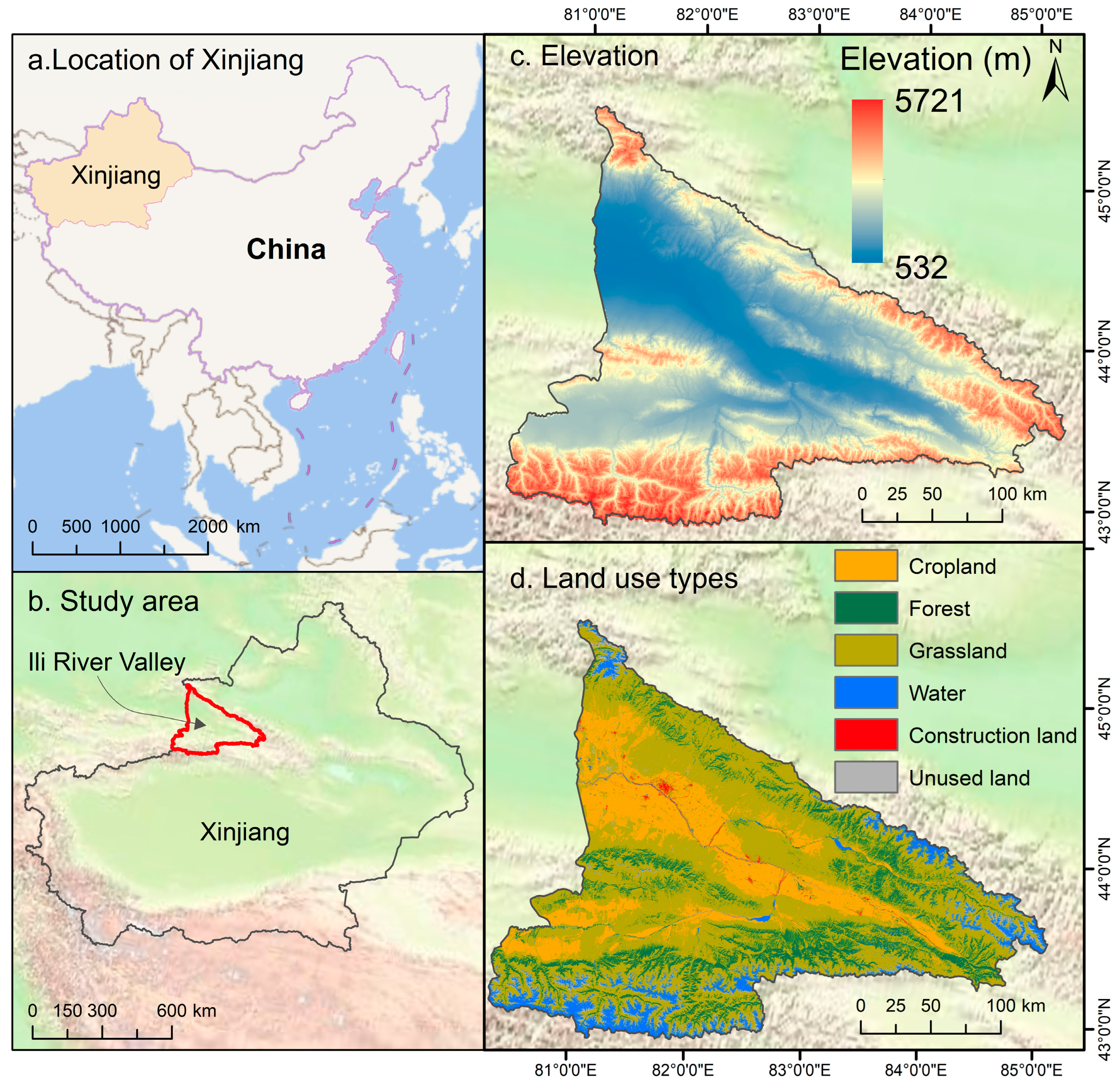
The Ili River Valley (80°09′–84°56′ E, 42°14′–44°50′ N) is a critical agricultural and ecological region in northwestern Xinjiang, China (Figure 1). This intermountain basin, covering approximately 5.46 × 10⁴ km² within the western Tianshan Mountains, features a distinct topographic funnel open to the west, which captures moisture-laden westerlies and creates a comparatively humid temperate continental climate. Mean annual precipitation ranges from 215 to over 800 mm, and the average temperature is 10.4 °C. Elevations span from 560 to over 5700 m, supporting vertical ecosystem zonation from valley farmlands to alpine meadows. The region contains over 2 × 10⁴ km² of natural grasslands and is a key grain-producing area, cultivating wheat, maize, and rice [25]. The total population of the Ili River Valley is 2.8484 million, and cultivated land accounts for one-sixth of the total land area. However, as a representative oasis ecosystem in an arid region, it faces significant ecological pressures from climate variability and intensifying human activities [26], making it a critical case for assessing farmland ecosystem health and sustainability.

2.2. Data Sources

This study integrates multi-source spatial datasets spanning 2000–2024 to assess ecosystem health. Prior to modeling, all data were unified to a common coordinate system (WGS_1984_UTM) and resampled to a 1 km resolution grid. The primary data sources are summarized as follows: (1) Land Use and Administrative Boundaries: Annual land use/cover data (30 m resolution) and county-level administrative boundary vectors were obtained from the Resources and Environmental Science Data Center (RESDC; https://www.resdc.cn). (2) Climate: Gridded data for mean annual precipitation, temperature, and potential evapotranspiration (1 km resolution) were acquired from the National Earth System Science Data Center (https://www.geodata.cn). (3) Topography and Vegetation: A 30 m resolution Digital Elevation Model (DEM) and annual Normalized Difference Vegetation Index (NDVI) data were sourced from the Geospatial Data Cloud (https://www.gscloud.cn), and slope was derived from the DEM. (4) Socio-economic Statistics: County-level population density and Gross Domestic Product (GDP) data were compiled from statistical yearbooks and the RESDC; nighttime light (NTL) data were obtained from the NOAA National Centers for Environmental Information (https://ngdc.noaa.gov). (5) Soil Properties: Key soil parameters (e.g., soil texture, root restricting layer depth, plant available water content) were derived from the Harmonized World Soil Database (HWSD v2.0) provided by the International Institute for Applied Systems Analysis and the Food and Agriculture Organization (https://www.iiasa.ac.at). (6) Infrastructure: Vector data for roads and railways were acquired from the National Platform for Common Geospatial Information Services (https://www.webmap.cn) and used to calculate distance-to-road raster layers.

2.3. Methods

2.3.1. Theoretical Framework

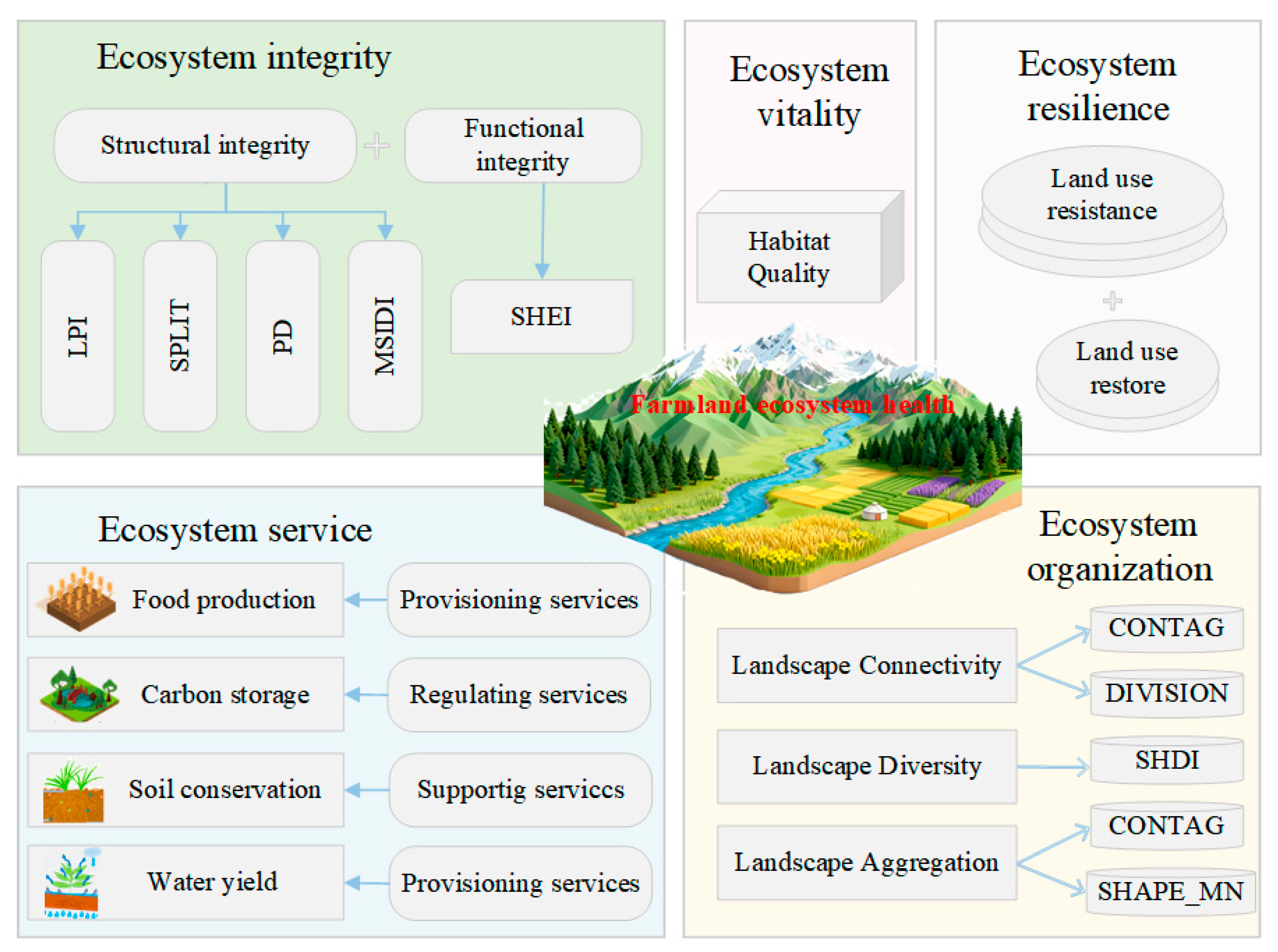
We established an improved ecosystem health assessment framework—the Vitality–Organization–Resilience–Ecosystem Services–Integrity (VOR-ES-I) model—to specifically tackle the erosion of ecosystem integrity in oasis farmlands, a critical issue stemming from high-intensity agricultural practices (Figure 2). While established frameworks like VORS have advanced the field, they often treat ecosystem integrity—the structural coherence, functional connectivity, and authenticity of ecological processes—as an implicit aspect of broader dimensions [19]. This can lead to assessments that capture high short-term productivity and service output but overlook underlying vulnerabilities arising from landscape homogenization, habitat fragmentation, or loss of biotic networks, which are defining features of oasis farmland ecosystems in arid regions. By elevating “Integrity” to a core, independent dimension alongside the traditional four, the VOR-ES-I model enables a more holistic and diagnostic evaluation. It explicitly quantifies the structural and functional foundations of the agricultural landscape through metrics of pattern, connectivity, and heterogeneity [27]. This integration ensures the assessment captures not only what the system provides but also how robustly it is structured to sustain these functions under stress, thereby offering a more complete foundation for sustainable management.

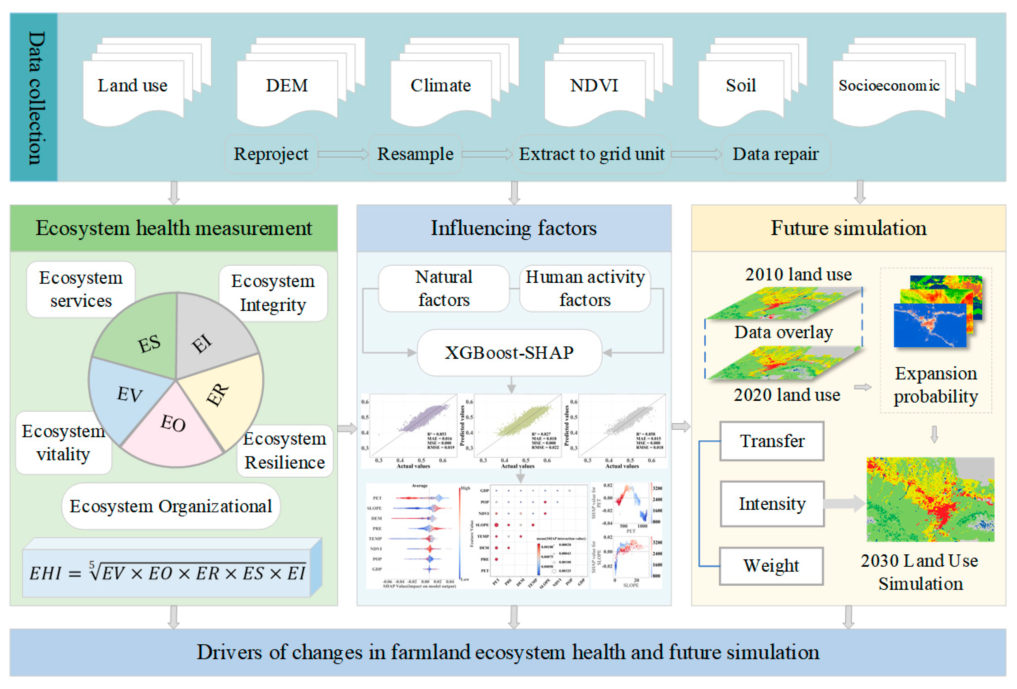
The analytical workflow to implement this framework comprises three main stages (Figure 3). First, the VOR-ES-I model is applied to conduct a multi-dimensional health assessment by calculating indices for the five core dimensions—Vitality (V), Organization (O), Resilience (R), Ecosystem Services (ES), and Integrity (I)—which are then synthesized into a composite Ecosystem Health Index to evaluate its spatiotemporal dynamics. Second, key drivers of health variation are identified and interpreted using the XGBoost-SHAP interpretable machine learning model, which quantifies the non-linear influences and relative importance of various natural and anthropogenic factors. Third, the driver–response relationships derived from the preceding analysis are coupled with the Patch-generating Land Use Simulation (PLUS) model to project the future (2030) spatial pattern of farmland ecosystem health under multiple development scenarios, thereby supporting forward-looking spatial planning and risk management.

2.3.2. Ecosystem Health Assessment

Based on the theoretical VOR-ES-I framework, this study quantitatively evaluates farmland ecosystem health in the Ili River Valley from five dimensions. All indicators within each dimension are considered equally crucial for a comprehensive assessment, so they are assigned equal weight and integrated using a multiplicative model [28]. To counteract the diminishing effect of multiplying fractional values, we calculate the fifth root of the product to derive the composite Ecosystem Health Index (EHI) [29,30]. Unlike the weighted additive model that allows compensation among dimensions, this approach penalizes extremely low-value dimensions and reflects the “short-board effect”—the overall EHI is significantly constrained by its weakest dimension. The specific formula is as follows:

$$EHI=\sqrt[5]{EV\times EO\times ER\times ES\times EI}$$

where EHI represents the Ecosystem Health Index for the Ili River Valley; EV is the ecosystem vitality index; EO is the ecosystem organization index; ER is the ecosystem resilience index; ES is the ecosystem service composite index; and EI is the ecosystem integrity index. Prior to integration, all individual indicator values were normalized to a range of 0–1 to eliminate dimensional and magnitude differences, ensuring comparability. For result interpretation and spatiotemporal analysis, the continuous EHI values were classified into five distinct health levels. The specific thresholds for ecosystem health levels were established through a combination of statistical data distribution and literature validation. Initially, the Natural Breaks (Jenks) method was applied to objectively identify the inherent clustering and breakpoints in the calculated EHI data, minimizing within-class variance and maximizing the variance between classes. Based on these statistical breakpoints, we performed minor adjustments to align with established ecological benchmarks reported in the previous literature [31,32]. This approach ensures that the classification is both statistically grounded in our study area’s specific conditions and comparable with broader ecosystem health assessments. The specific classification thresholds are as follows: Low (0–0.25), Relatively Low (0.25–0.35), Medium (0.35–0.45), Relatively High (0.45–0.55), and High (0.55–1.0). The calculation methods for each dimension are detailed below.

(1)

Ecosystem Vitality (EV)

Ecosystem vitality reflects the metabolic capacity and primary productivity of the system. While metrics like Net Primary Productivity (NPP) and the Normalized Difference Vegetation Index (NDVI) are commonly used [12], this study selects habitat quality as the proxy for EV. This choice is based on its capacity to reflect not only the availability of resources for organism survival and reproduction but also the crucial role of biodiversity within the system, offering a more integrative measure of ecological vitality for the intensively managed farmland landscape [33]. Habitat quality was calculated using the InVEST model, with the formula as follows [34]:

$$Q_{xi}=H_i\times \left(1-{\displaystyle \frac{D_{xi}^z}{D_{xi}^z+k^z}}\right)$$

where $Q_{xi}$ represents habitat quality of grid cell $x$ in land use type $i$; $H_i$ represents habitat suitability of land use type $i$; $D_{xi}$ represents habitat degradation index of grid cell $x$ in land use type $i$; $k$ denotes half-saturation constant; and $z$ is the constant determined by the model.

(2)

Ecosystem Organization (EO)

EO characterizes the structural stability and complexity of the landscape [35]. It is quantified by integrating key landscape pattern indices grouped into three dimensions: landscape heterogeneity (LH), landscape connectivity (LC), and landscape shape (LS) [19,36]. Specifically, LH is represented by Shannon’s Diversity Index (SHDI); LC is represented by the Connectance Index (CONNECT), Contagion Index (CONTAG), and Landscape Division Index (DIVISION); and LS is represented by the Mean Shape Index (SHAPE_MN).

To determine the weights, we first assigned dimension-level weights based on the previous literature [19,37], which emphasizes that connectivity plays the most critical role in maintaining ecological organization, followed by heterogeneity, and then shape. Accordingly, the dimensions LC, LH, and LS were assigned weights of 0.45, 0.35, and 0.20, respectively. These dimension weights were then equally distributed among the indices within each dimension to obtain the final index weights: SHDI (0.35/1 = 0.35), CONNECT, CONTAG, and DIVISION (0.45/3 = 0.15 each), and SHAPE_MN (0.20/1 = 0.20). Specifically, these landscape metrics were computed via a moving window approach within Fragstats, with a window size of 3000 m and a step size of 5000 m. Forest, grassland, water bodies and cropland were designated as foreground classes, and the resulting continuous outputs were subsequently resampled into a raster at 1 km resolution. The EO formula is:

$$EO=0.35\times SHDI+0.15\times CONNECT+0.2\times SHAP{E}_{MN}+0.15\times CONTAG+0.15\times DIVISION$$

(3)

Ecosystem Resilience (ER)

ER denotes the capacity of an ecosystem to resist disturbances and recover its structure and function [31]. It is assessed by assigning resistance and resilience coefficients to different land use/cover types, reflecting their inherent ability to withstand and rebound from stressors. The coefficients were determined based on the specific environmental conditions of the Ili River Valley and calibrated values from prior studies in similar ecological contexts [33,37,38]. For example, forests have high resilience (1.0) due to their complex structure and recovery potential but lower resistance (0.6) to disturbances like fire, while grasslands exhibit high resistance (0.8) to grazing or drought but slightly lower resilience (0.7) due to simpler ecological structure. These coefficients reflect the trade-offs between an ecosystem’s ability to withstand (resistance) and recover from (resilience) disturbance, as defined in ecological resilience theory (e.g., [31]). ER is calculated as the area-weighted sum of these coefficients for all land use types, with the formula as follows:

$$ER=0.4\times {\sum }_{i=1}^n{L}_i\times C_{resis,i}+0.6\times {\sum }_{i=1}^n{L}_i\times C_{resil,i}$$

where $ER$ represents regional ecosystem resilience; $C_{resis,i}$ and $C_{resil,i}$ denote resistance coefficient and resilience coefficient of land use type $i$ (

Table 1. Resilience and resistance coefficients for each land use type.

Land Use Type	Cropland	Forest	Grassland	Water Body	Construction Land	Unused Land
Resilience coefficient	0.5	1	0.7	0.8	0.3	0.2
Resistance coefficient	0.3	0.6	0.8	0.7	0.2	0.1

); $L_i$ is the area proportion of land use type $i$; and $n$ is the number of land use types.

(4)

Ecosystem services (ES)

The ecosystem service composite index (ESCI) measures the multiple benefits provided by the ecosystem to human society [12]. Four critical services for the agricultural region were quantified and integrated: Soil Conservation, Water Yield, Carbon Storage, and Food Production. The individual service values were first normalized independently for each year and then summed with equal weights to derive the ESCI. The formula is as follows:

$${ES}_b={\displaystyle \frac{ES-{ES}_{min}}{{ES}_{max}-{ES}_{min}}}$$

$$ESCI={\sum }_{i=1}^n{ES}_{bi}$$

where ${ES}_b$ is the normalized value of each ecosystem service, ES is the original value of the ecosystem service, and ${ES}_{max}$ and ${ES}_{min}$ denote the maximum and minimum values of the service, respectively. $ESCI$ represents the ecosystem services composite index, and ${ES}_{bi}$ is the normalized result of the $i-th$ type of ecosystem service. Detailed calculation methods for each service type are shown in

Table 2. Calculation methods and parameter descriptions for different ecosystem service types.

ES Type	Formulas and Descriptions	References
Soil conservation (SC)	${\mathrm{A}}_{\mathrm{c}}={\mathrm{A}}_{\mathrm{p}}-{\mathrm{A}}_{\mathrm{v}}=\mathrm{R}\times \mathrm{K}\times \mathrm{L}\mathrm{S}\times 1-\mathrm{C}\times \mathrm{P}$ ${\mathrm{A}}_{\mathrm{c}}$: soil conservation amount; ${\mathrm{A}}_{\mathrm{p}}$: potential soil erosion amount; ${\mathrm{A}}_{\mathrm{v}}$: actual soil erosion amount; $\mathrm{R}$: rainfall erosivity factor; K: soil erodibility factor; LS: slope length and steepness factor; C: vegetation cover factor; P: soil and water conservation practice factor.	InVEST User Guide [39]
Water yield (WY)	${WY}_i=\left(1-{\displaystyle \frac{A_{\mathrm{E}\mathrm{T},i}}{P_i}}\right)P_i$ ${WY}_i$: annual water yield for each grid cell; $A_{\mathrm{E}\mathrm{T},i}$: annual actual evapotranspiration for pixel; $P_i$: annual precipitation on pixel $i$.
Carbon Storage (CS)	$C_{total}=C_{above}+C_{below}+C_{soil}+C_{dead}$ $C_{total}$: total ecosystem carbon storage; $C_{above}$: aboveground carbon density; $C_{below}$: belowground carbon density; $C_{soil}$: soil organic carbon density; $C_{dead}$: dead organic carbon density.
Food Production (FP)	${CP}_i={\displaystyle \frac{{NDVI}_i}{{NDVI}_{sum}}}\times {CP}_{sum}$ ${CP}_i$: grain yield of grid cell $i$; ${CP}_{sum}$: total grain yield of the study area; ${NDVI}_i$: NDVI of grid cell $i$; ${NDVI}_{sum}$: total NDVI of the study area.

.

(5)

Ecosystem Integrity (EI)

EI is introduced as an independent dimension to explicitly evaluate the structural and functional coherence of the ecosystem. It is synthesized from indicators representing both functional and structural integrity: functional integrity was measured by Shannon’s Evenness Index (SHEI), reflecting the equitable distribution of area among patch types (weight = 0.20). Structural integrity was assessed through a combination of three complementary indices: the Largest Patch Index (LPI, weight = 0.30) representing dominance; the Splitting Index (SPLIT, inverse, weight = 0.15) and Patch Density (PD, inverse, weight = 0.15) both indicating fragmentation (inverse values imply higher integrity with lower fragmentation); and the Modified Simpson Diversity Index (MSIDI, weight = 0.20) for complexity of community structure.

The rationale for designating EI as an independent dimension is rooted in the following considerations. Specifically, it is necessary to establish clear conceptual and methodological boundaries between EI and the other four dimensions—particularly EO, as both utilize landscape metrics. While EO characterizes the geometric complexity and spatial configuration of the landscape (i.e., how intricately elements are arranged), EI explicitly quantifies the un-fragmented coherence and core retention of the system (i.e., how severely the original ecological matrix has been dissected by anthropogenic activities). A highly intensified agricultural matrix may exhibit high EO due to complex boundary shapes and mixed land use types, yet suffer from critically low EI due to severed ecological networks. The specific indicators within EI were deliberately selected to capture this “anti-fragmentation” baseline that remains blind to V, R, ES, and EO:

First, the LPI identifies the presence of un-fragmented core habitats. Unlike ER—which assigns uniform recovery coefficients based solely on land-cover types—LPI reveals the spatial structural guarantee of resilience. A forest area fragmented into numerous small patches retains the same theoretical ER coefficient as a contiguous one, but LPI uniquely captures the loss of the spatial anchors necessary to sustain this resilience.

Second, PD and the SPLIT, applied inversely here, serve as direct diagnostic tools for physical severance. While EO uses metrics like CONNECT to evaluate potential spatial adjacency, PD and SPLIT ignore land cover identities to quantify the sheer intensity of physical dissection caused by infrastructure and land conversion. They measure the “density of ecological scars”, an aspect of structural degradation not represented by EO’s focus on heterogeneity.

Finally, SHEI and the MSIDI are employed not merely to commend diversity, but to detect the “monoculture trap”. In the context of oasis farmlands, low SHEI signals the absolute dominance of a single artificial matrix (e.g., extensive cropland) over natural communities. This specifically captures a structural vulnerability that ES and EV fail to diagnose: a landscape can exhibit high crop yield (ES) and vegetation cover (EV) while experiencing a catastrophic loss of baseline integrity due to the homogenization of community structure.

The composite EI formula is

$$EI=0.2\times SHEI+0.3\times LPI+0.15\times \left({\displaystyle \frac{1}{{SPLIT}_{norm}}}\right)+0.15\times \left({\displaystyle \frac{1}{{PD}_{norm}}}\right)+0.2\times MSIDI$$

where _$norm$ denotes Min-Max normalization to retain comparable scales and avoid negative values.

2.3.3. Driving Factor Analysis Based on XGBoost-SHAP

To identify and quantify the driving mechanisms, this study employed the XGBoost machine learning algorithm in conjunction with the SHAP interpretability framework. Based on the ecological characteristics of the study area and data availability, eight potential driving factors across multiple dimensions were selected for analysis: Topography (Elevation/DEM, Slope), Climate (Annual Precipitation/PRE, Annual Mean Temperature/TEMP, Potential Evapotranspiration/PET), Vegetation Condition (Normalized Difference Vegetation Index/NDVI), and Human Activity (Population Density/POP, Gross Domestic Product/GDP). These factors collectively represent the key natural constraints and anthropogenic pressures influencing the farmland ecosystem. Fine-scale management factors (e.g., fertilizer use) were excluded due to the lack of continuous spatial raster data across the 24-year time series.

XGBoost is an advanced ensemble learning algorithm based on gradient-boosted decision trees, excelling at modeling complex non-linear relationships and capturing multi-variable interaction effects while remaining robust against overfitting via built-in regularization techniques [40]. In this study, the EHI served as the dependent variable, and the eight driving factors were used as independent variables. The dataset was randomly partitioned into a training set (70%) and a testing set (30%).

A five-fold cross-validation procedure combined with a grid search was employed on the training set to optimize the model’s hyperparameters, thereby enhancing generalization performance. The optimal configuration yielded a learning rate of 0.1, a max_depth of 6, and n_estimators of 500. The predictive accuracy and robustness of the optimized XGBoost model were evaluated using the coefficient of determination (R²), Mean Absolute Error (MAE), Mean Squared Error (MSE), and Root Mean Square Error (RMSE) [41].

To overcome the “black-box” nature of complex machine learning models and gain mechanistic insights, the SHAP method was applied to interpret the trained XGBoost model. Grounded in cooperative game theory, SHAP quantifies the marginal contribution of each feature (driving factor) to every individual prediction, decoupling predictive drivers from mere index composition to provide both global and local interpretability [42]. The analysis yields three key insights: (1) the feature importance ranking, which indicates the relative influence of each driver on the EHI; (2) the SHAP dependency plots, which reveal the direction (positive or negative) and the nature (linear, non-linear, threshold) of the relationship between each factor’s value and its impact on the EHI; and (3) the analysis of interaction effects, where SHAP values can elucidate how the impact of one factor may depend on or be modified by the value of another. This combined XGBoost-SHAP approach allows for a transparent and in-depth analysis of the dominant drivers, their individual effects, and their interactions in shaping farmland ecosystem health dynamics.

2.3.4. Future Land Use Simulation and Ecosystem Health Projection

To project the future trajectory of farmland ecosystem health under different development pathways, this study employed the Patch-generating Land Use Simulation (PLUS) model. The PLUS model integrates a Land Expansion Analysis Strategy (LEAS) module and a CA model based on a multi-class random seed (CARS) mechanism, which is adept at capturing the complex, patch-level transitions of multiple land use types under the influence of diverse drivers [43].

(1)

Driving factor selection

Drawing on the principles of data accessibility, quantifiability, and their established influence on land use change, 13 spatial driving factors across four categories were selected. Unlike the macro-scale ecological gradients used for XGBoost, the PLUS model necessitates these additional fine-grained spatial variables (e.g., specific road distances) to capture the localized friction dictating precise land use conversion locations. These cover natural geographic factors, namely elevation (DEM) and slope; climate and vegetation factors, including annual mean temperature, annual precipitation, and NDVI; accessibility factors, specifically Euclidean distances to rivers, highways, national roads, railways, and general roads; and socio-economic factors, which are population density and Gross Domestic Product (GDP) density. The socio-economic data were collected for 2000, 2010, and 2020 to match the calibration and simulation timeframe of the PLUS model. All factor layers were standardized to a 1 km resolution raster grid.

(2)

Model calibration and scenario definition

The simulation process was conducted in two stages. First, the LEAS module was utilized to extract the land use expansion characteristics and development probabilities for each land use type between 2010 and 2020. Second, the CARS module was applied to simulate the spatial pattern of land use for the target year 2030, incorporating neighborhood competitive mechanisms and stochastic patch generation.

Three distinct scenarios were designed to reflect different policy orientations and development priorities. The specific parameter adjustments for the land use conversion probabilities in the CARS module are defined as follows:

Scenario 1 (S1): Natural Development scenario. This scenario assumes no exogenous policy intervention. Land use changes are projected based solely on the transition trends and probabilities derived from the 2010–2020 period, serving as a baseline for comparison.

Scenario 2 (S2): Farmland Protection scenario. This scenario prioritizes food security and arable land conservation. Following standard spatial simulation practices where qualitative policy objectives are translated into relative quantitative shifts, the transition probabilities from farmland to grassland and water bodies were reduced by 40%, while the probability for unused land to convert to farmland was increased by 30% as an exploratory boundary test. These adjustments aim to curb the loss of cultivated land and encourage the reclamation of suitable unused areas.

Scenario 3 (S3): Urban Development scenario. This scenario emphasizes socio-economic growth and urban expansion while considering the need to balance development with ecological and agricultural constraints. Accordingly, the transition probabilities from both farmland and grassland to construction land were increased by 10%. Conversely, to stabilize existing urban areas and discourage inefficient land use reversion, the probabilities for construction land to convert back to farmland or grassland were reduced by 30%.

For all scenarios, key natural reserves and ecologically sensitive areas within the Ili River Valley were designated as restricted expansion zones where land use conversion was prohibited.

(3)

Model validation and future EHI assessment

The model’s performance was validated by simulating the 2020 land use pattern using 2020 and 2010 as the base year and the calibrated parameters. The simulated 2020 map was compared with the actual observed map using the Overall Accuracy and the Kappa coefficient to ensure reliability before projecting to 2030.

Subsequently, the simulated land use maps for 2030 under the three scenarios served as the foundational input for forward-looking ecosystem health assessment. The previously established VOR-ES-I evaluation framework (Section 2.3.2) was applied to these future land use patterns, along with projected climatic and socio-economic data where applicable, to calculate the future EHI. The spatiotemporal trends and differences in EHI under the contrasting scenarios were then analyzed.

3. Results

3.1. Spatiotemporal Dynamics of Ecosystem Health

3.1.1. Ecosystem Health Indicators

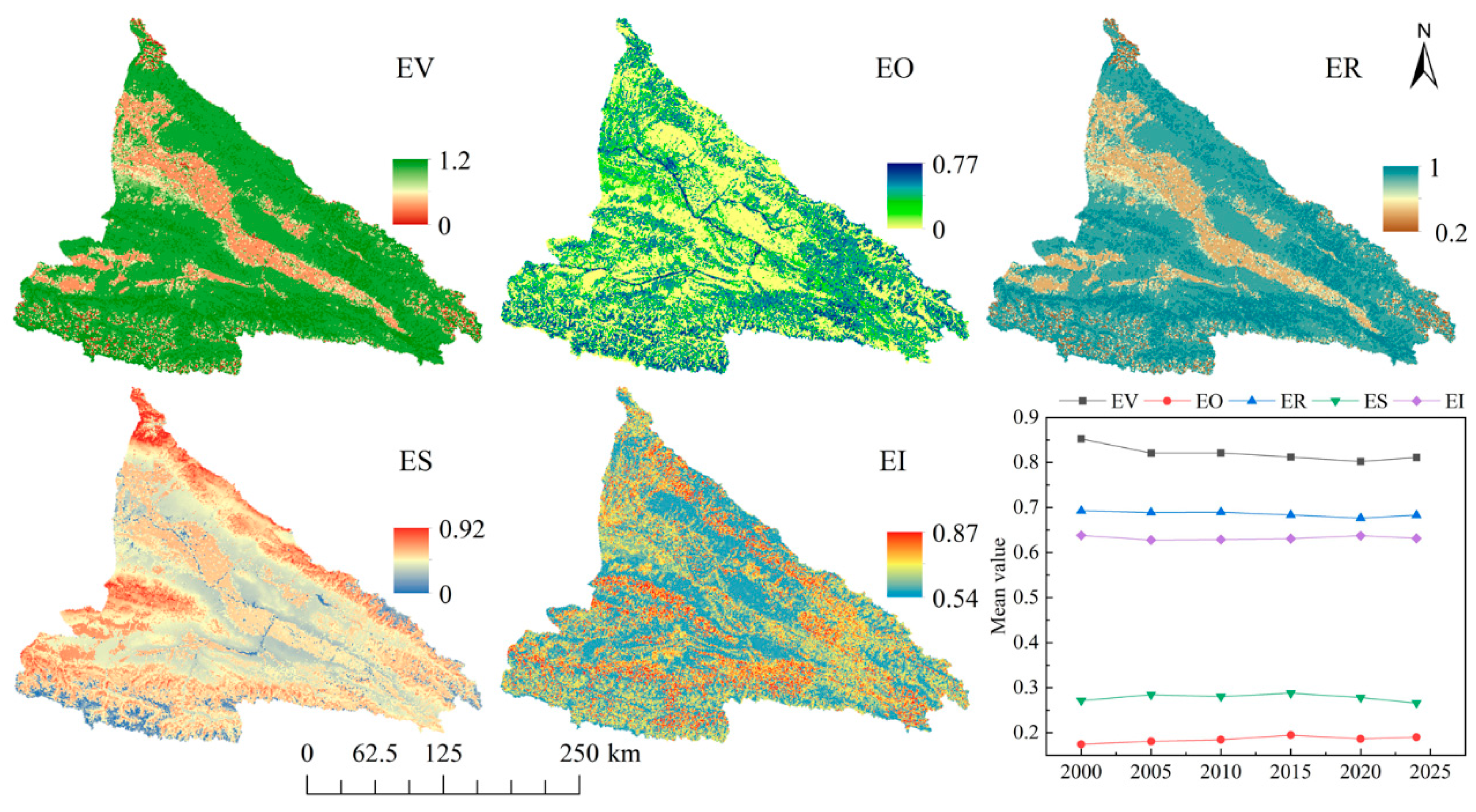
The five core indicators of ecosystem health exhibited distinct spatiotemporal dynamics from 2000 to 2024 in the Ili River Valley (Figure 4).

Ecosystem vitality (EV) showed an overall declining trend, despite minor fluctuations, decreasing from 0.852 in 2000 to 0.811 in 2024, a reduction of 4.81%. Spatially, areas of high vitality were predominantly located in the forest and grassland landscapes of the high-altitude northern and southern mountain regions. In contrast, the central plain of the valley, dominated by cropland and construction land, constituted a low-vitality zone. Over the past two decades, a marked decline in EV was observed in the intensively cultivated areas, particularly in the central–western part of the valley (Figure S1).

Ecosystem organization (EO) demonstrated an overall increasing trend, rising from 0.174 in 2000 to 0.190 in 2024, with a peak value of 0.194 reached in 2015. Spatially, a clear north–south gradient was observed, with EO values in the northern sector of the basin generally lower than those in the south. This pattern aligns with the region’s distinctive west-opening trumpet-shaped topography. Higher EO values were observed in the southern portion of this topography, which encompasses the east–southwest-trending mountains and their adjacent piedmont plains, compared to the northern portion with east–northwest-trending mountains and plains. Notably, the northern mountainous regions experienced a significant increase in EO over the study period (Figure S2).

Ecosystem resilience (ER) experienced a slight overall decrease of 1.44%, declining from 0.693 in 2000 to 0.683 in 2024; given the limited number of temporal observations (six periods), this minor fractional change is more effectively interpreted through its spatial heterogeneity than traditional temporal trend tests. Similar to EV, high-resilience areas were concentrated in the forest and grassland ecosystems of the high-altitude northern and southern mountains, while the central plain was characterized by lower resilience. Temporally, ER declined significantly in the high-altitude areas of the northeast and southeast. Conversely, a restorative increase was detected in the northwestern corner of the Tianshan Mountains within the valley (Figures S3 and S4).

Ecosystem services (ES) displayed a pattern of initial increase followed by a decrease. The ES composite index rose from 0.271 in 2000 to a peak of 0.287 in 2015, before gradually declining to 0.266 by 2024. Spatially, high-value ES areas were primarily located in the northwestern corner and the central–western part of the valley, whereas the high-altitude regions of the east–southwest-trending Tianshan Mountains generally had lower ES values. Over time, ES decreased in the southern Tianshan Mountains, central-western, and southeastern areas, but increased in the northwestern low-altitude plains (Figure S5).

Ecosystem integrity (EI) followed a trajectory of initial decline and subsequent recovery. The index decreased from 0.638 in 2000 to 0.628 in 2005, before gradually rising to 0.637 by 2024. Spatially, integrity was generally higher in the south than in the north, and higher in the east and mountainous areas than in the west and plains. Notably, the plain–mountain transition zones in the study area showed uniformly low EI, whereas their EV and ER levels were comparatively high. The most noticeable increases in EI occurred in the central–western part of the valley opening and the eastern plains during the study period (Figure S6).

3.1.2. Ecosystem Health

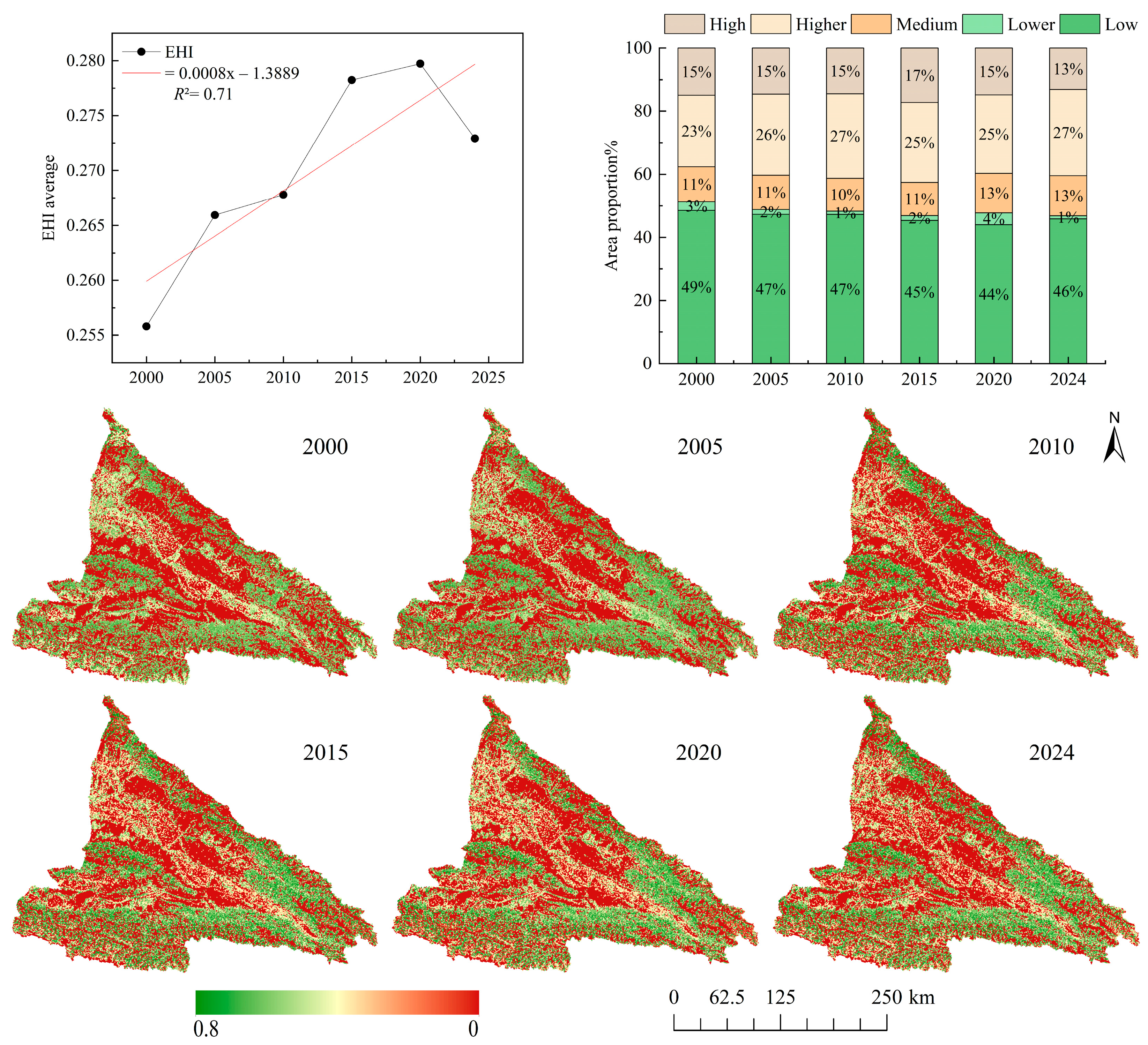
Building upon the five constituent indicators, the composite Ecosystem Health Index (EHI) was calculated for the Ili River Valley from 2000 to 2024 and classified into five health levels (Figure 5). Spatially, the EHI exhibited a pronounced topographic gradient. Areas of high ecosystem health were predominantly distributed in the high-altitude mountainous regions, whereas the central plains were characterized by significantly lower health levels. This pattern is likely attributable to minimal human disturbance in the remote highlands. In terms of landscape types, forest landscapes generally sustained the highest EHI, followed by cropland and construction land. Grassland ecosystems exhibited the lowest composite health scores.

Temporally, the basin’s mean EHI demonstrated an overall upward trend, increasing from 0.2565 in 2000 to 0.2732 in 2024, with intermediate values of 0.266 (2005), 0.2681 (2010), 0.2787 (2015), and 0.2802 (2020). This improvement was reflected in the shifts among health categories. The areal proportion of “High” health zones decreased from 15.1% to 13.2%, while the “Relatively High” category expanded notably from 22.7% to 27.3%. The “Medium” category also increased from 10.5% to 12.8%. Concurrently, the share of “Low” and “Relatively Low” health areas contracted from 48.6% to 45.8% and from 3.1% to 0.9%, respectively. According to the transition matrix (

Table 3. Transition matrix of ecosystem health levels between 2000 and 2024.

2024\2000 (km2)	Low	Lower	Medium	Higher	High	Total
Low	19,876	758	1776	2018	514	24,942
Lower	46	62	202	82	120	512
Medium	2127	473	2764	1565	274	7203
Higher	3779	174	1196	6915	2753	14,817
High	691	35	129	1803	4538	7196

), the overall improvement was driven by net upward transfers: for instance, 473 km² from “Relatively Low” to “Medium”, 1196 km² from “Medium” to “Higher”, and 1803 units from “Higher” to “High”, while some degradation from “High” to “Higher” (2753 km²) also occurred. These shifts indicate that the overall improvement was primarily driven by the expansion of “Relatively High” and “Medium” zones and the contraction of poorer health areas, particularly evident in the southeastern and central–western parts of the valley.

Overall, the ecosystem health of the Ili River Valley showed a significant improving trend. Statistically, 58.46% of the region experienced marked health enhancement, whereas only 16.23% exhibited a decline (p < 0.05), underscoring a positive trajectory in ecological conditions over the past two decades.

3.2. Driving Factors Analysis

3.2.1. Model Performance Evaluation

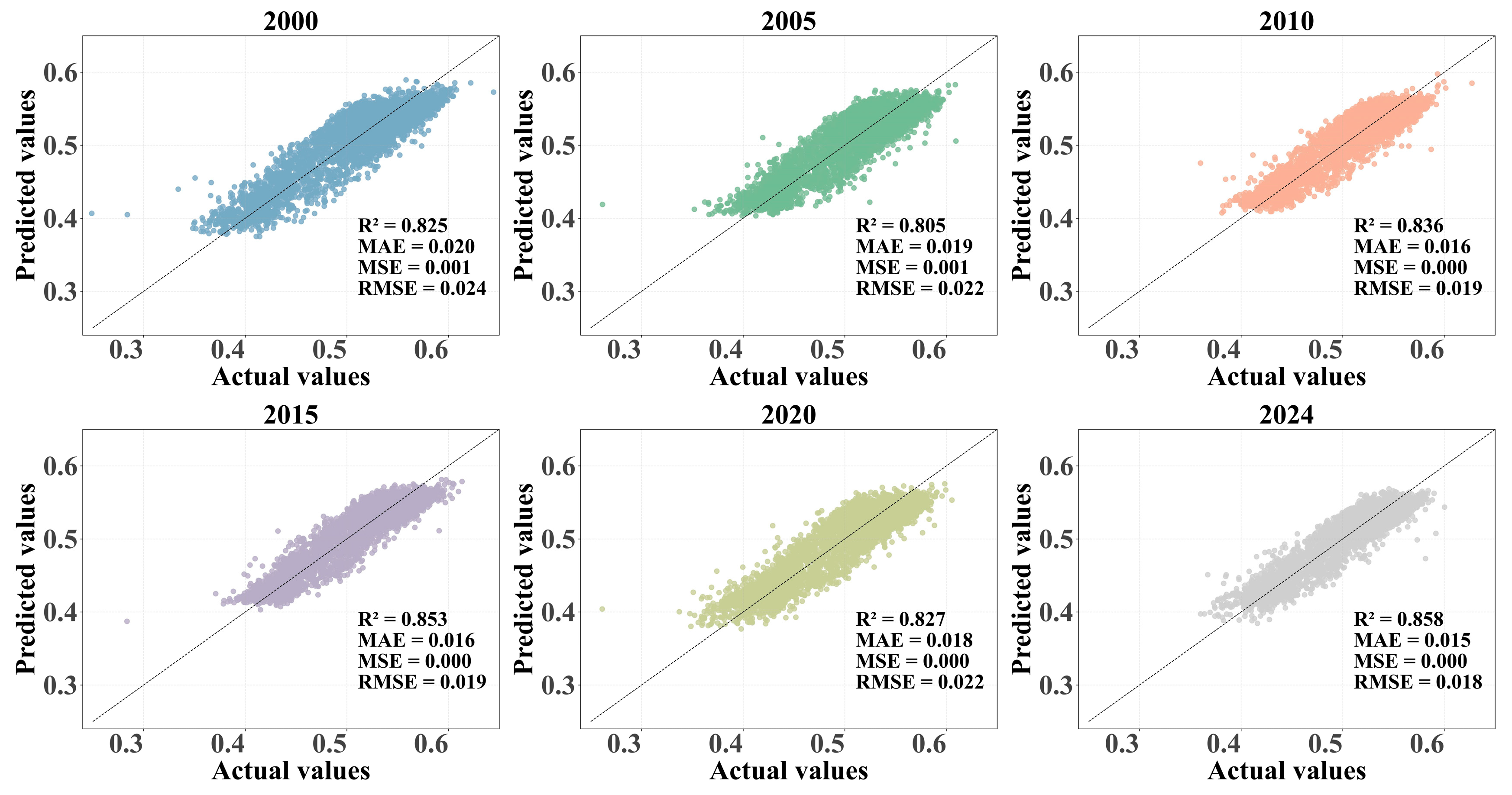
To unravel the multi-dimensional driving mechanisms behind the EHI in the Ili River Valley, an XGBoost regression model was constructed and interpreted using the SHAP framework. As shown in Figure 6, the XGBoost model, optimized via grid search, demonstrated excellent and stable performance on the test set from 2000 to 2024. The coefficient of determination (R²) ranged between 0.805 and 0.858, indicating a strong goodness of fit. The low values of RMSE (0.018), MAE (0.015), and MSE (0.001) collectively confirmed the model’s high predictive accuracy and robustness. This performance validates the model’s efficacy in capturing the complex, non-linear relationships between EHI and its driving factors, providing a solid foundation for the subsequent SHAP-based quantification of individual factor contributions and interaction effects.

3.2.2. Identification and Evolution of Dominant Driving Factors

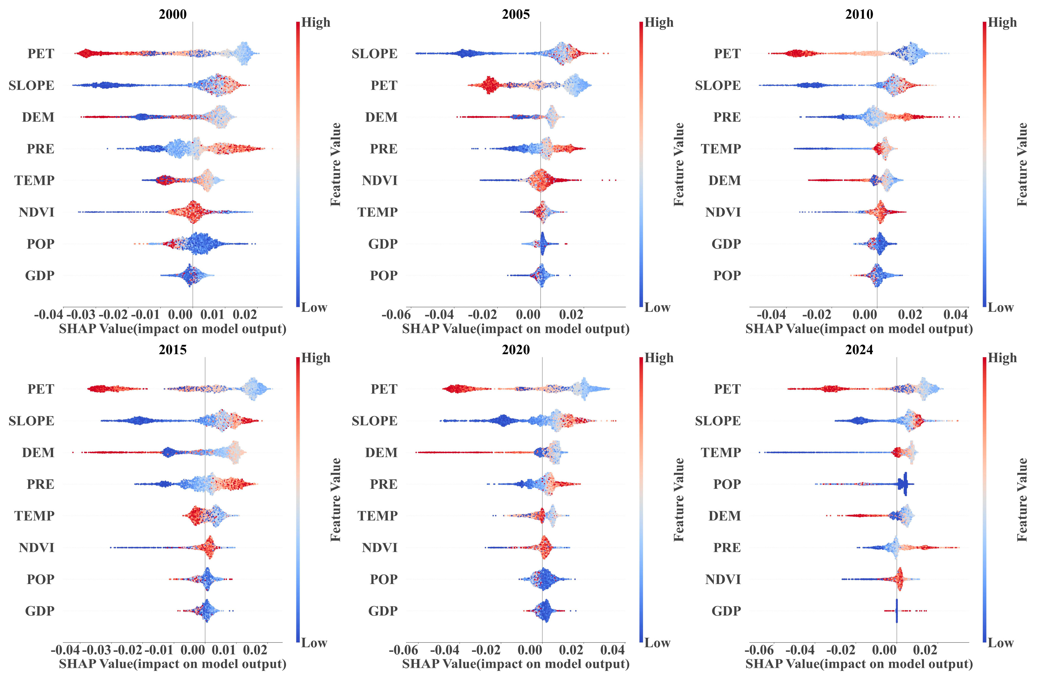
The SHAP analysis revealed the relative importance and temporal evolution of key driving factors from 2000 to 2024 (Figure 7). Potential evapotranspiration (PET) and slope consistently ranked as dominant factors throughout the period, emerging as the core drivers by 2024. The influence of precipitation (PRE) remained relatively stable from 2000 to 2015 but showed a slight weakening from 2020 to 2024, suggesting its effect may have plateaued or become modulated by other factors. Conversely, the importance of temperature (TEMP) exhibited a gradual increase from 2000 to 2024, highlighting the growing significance of thermal conditions under global warming. Although population density (POP) and Gross Domestic Product (GDP) increased rapidly between 2000 and 2010, their absolute contribution magnitudes remained low, indicating a limited direct influence on EHI compared to natural factors.

Regarding the direction of influence, PET and elevation (DEM) predominantly showed negative correlations with EHI, whereas slope, NDVI, and PRE generally exhibited positive correlations. The relationship for other factors, such as temperature, was more complex, potentially promoting ecosystem processes within a certain range but switching to a negative impact under extreme high temperatures.

3.2.3. Synergistic Interaction Networks and Threshold Characteristics

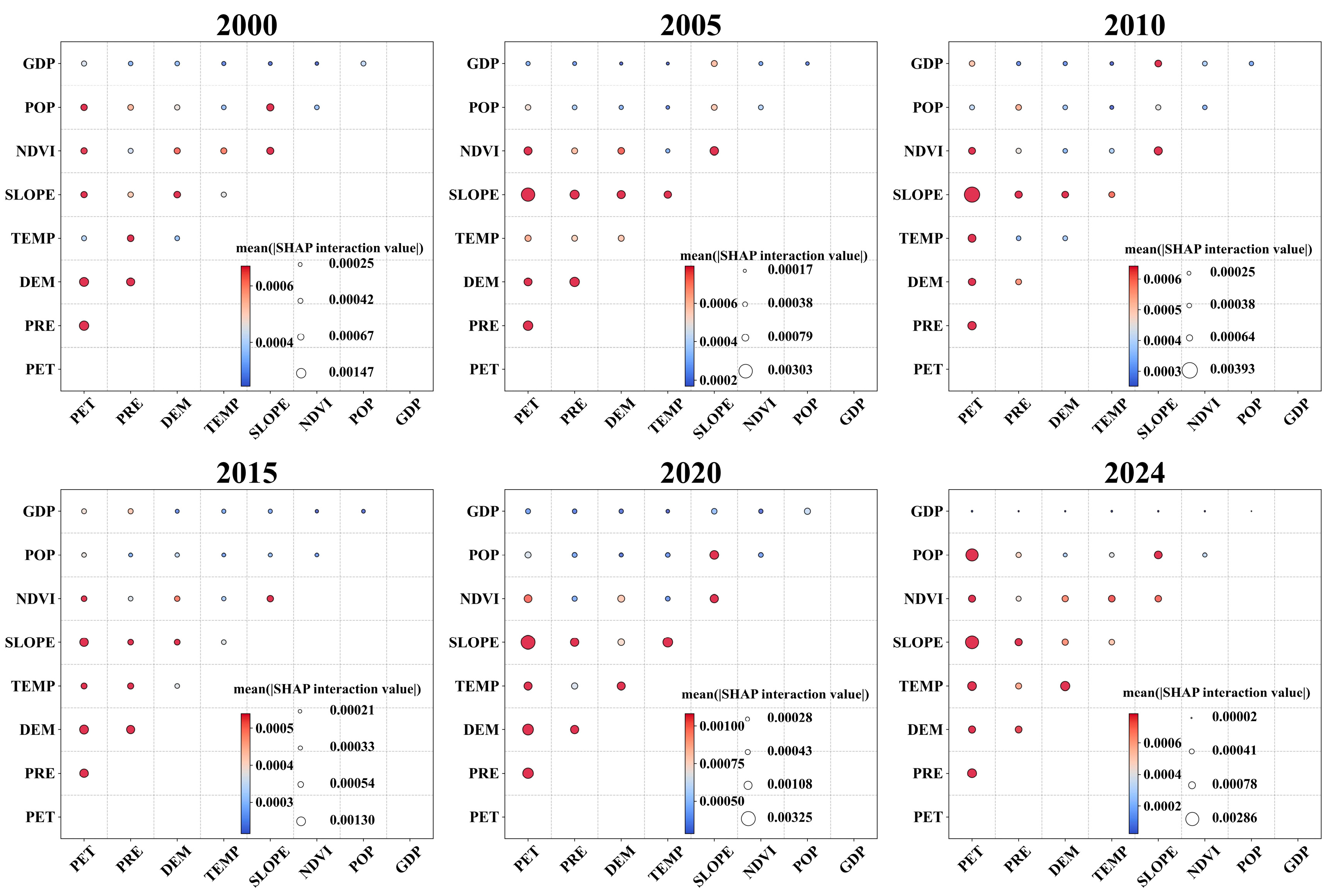
Analysis of interaction effects uncovered that the combined influence of PET, POP, PRE, and DEM on EHI was particularly prominent. Between 2005 and 2024, the interaction between PET and slope was the most significant, with SHAP interaction values ranging from 0.0030 to 0.0039. During the entire study period, there were interactions between PRE and PET, DEM and PRE, as well as slope and DEM, with their SHAP interaction values ranging from 0.0005 to 0.0008. Notably, some factors with weak individual effects (e.g., POP, with individual SHAP value < 0.0001) exhibited a substantially amplified influence when interacting with others (e.g., the slope × POP interaction reached 0.0011 in 2005). This underscores the “multi-factor synergistic driving” characteristic intrinsic to farmland ecosystems, where the collective effect of factors exceeds the sum of their individual impacts (Figure 8).

3.2.4. Interaction Modes and Effectiveness Thresholds

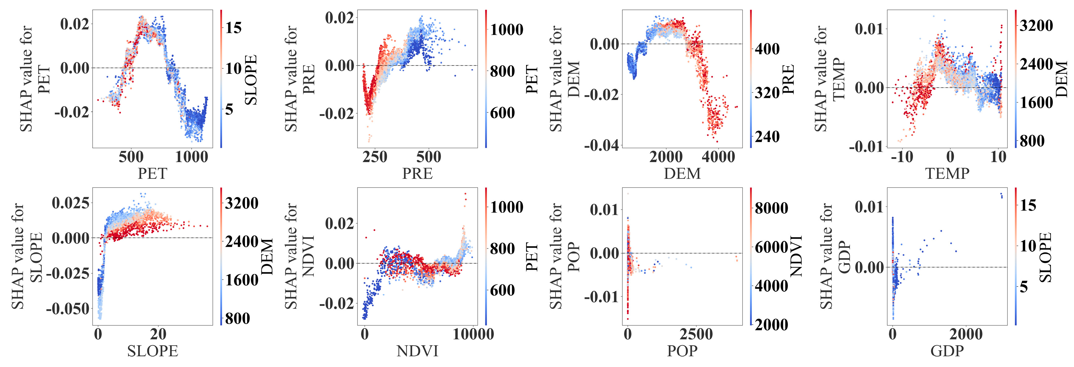
To probe the dynamic interactions among driving factors, two-dimensional SHAP interaction dependence plots were analyzed (Figure 9), revealing distinct non-linear patterns and effectiveness thresholds.

For the PET and slope interaction, the SHAP value formed an inverted U-shape relative to PET. EHI increased with PET until a threshold of approximately 557 mm, after which it declined. Within the intermediate PET range (550–700 mm), the interaction with Slope was most apparent: here, higher slope values mitigated the negative impact of rising PET on EHI, whereas lower slopes exacerbated it. The interaction between PRE and PET exhibited a V-shaped pattern. The combined effect was negative until PRE reached about 205 mm, turning positive thereafter. The most pronounced positive synergistic effect occurred within the PRE range of 250–457 mm. The DEM and PRE interaction also showed an inverted U-shape concerning DEM. The interaction was stable and positive within the mid-elevation band (1500–2500 m). Outside this range, the relationship shifted, being positive below 1500 m and negative above 2500 m. The slope and DEM interaction revealed that while EHI generally had a non-linear positive relationship with slope alone, its interaction with DEM was negative. This indicates that the beneficial effect of increased slope on EHI can be attenuated at higher elevations. The network depicting the interaction strengths among other drivers is shown in (Figure S7).

3.3. Projection of Future Ecosystem Health Under Multiple Scenarios

Based on PLUS model simulations of land use in 2030, the future trajectory of the EHI for the Ili River Valley was assessed under three development scenarios. The results indicate that distinct land management policies will lead to significant divergence in ecological outcomes.

3.3.1. Scenario Comparison of Overall Health Levels

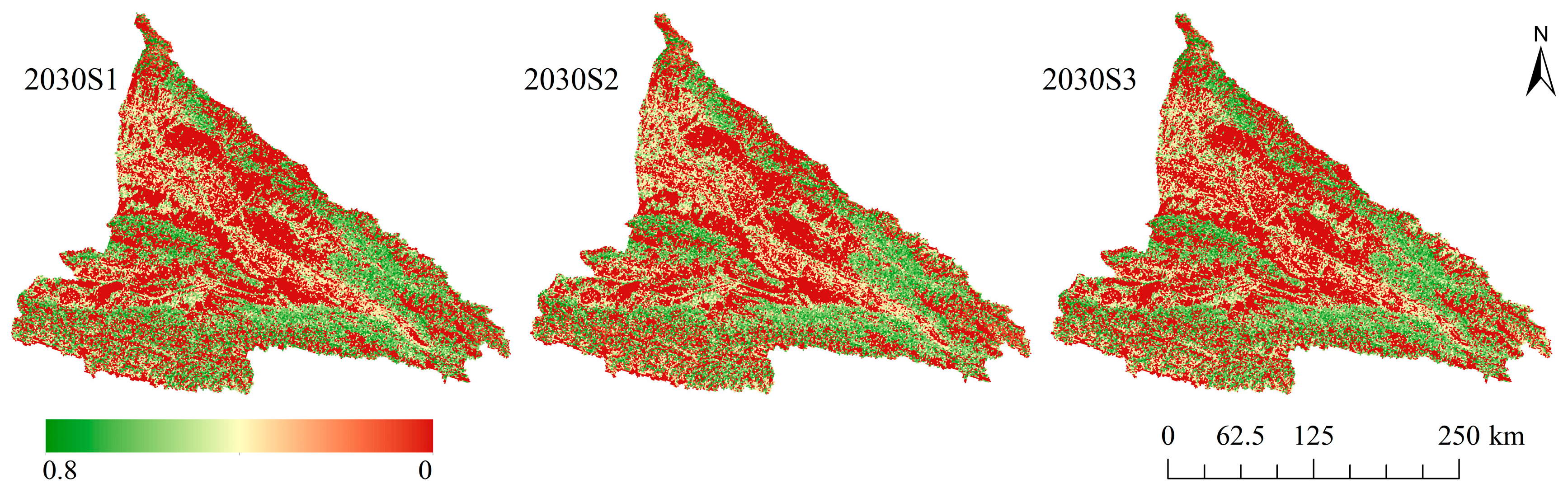
Compared to the 2024 baseline (mean EHI = 0.2732), the Farmland Protection scenario (S2) offers the best ecological prospects, with the regional mean EHI expected to rise to 0.290, a 6.2% improvement. Under the Natural Development scenario (S1), the mean EHI is projected to remain at 0.2731, suggesting a continuation of the current status quo without substantial improvement or decline. In contrast, the Urban Development scenario (S3) projects a decline in the mean EHI to 0.267, highlighting the potential ecological risks associated with expansive urbanization.

3.3.2. Areal Shifts and Spatial Reconfiguration of Health Levels

The transfer of area among ecosystem health levels across scenarios is summarized in

Table 4. Projected area (km²) and proportion (%) of ecosystem health levels and mean EHI under different scenarios.

Health Level	2024 (Baseline)	S1 (Natural Dev.)	S2 (Farmland Prot.)	S3 (Urban Dev.)
High	7226 (13.2%)	10,002 (18.3%)	14,302 (26.2%)	14,831 (27.1%)
Relatively High	14,880 (27.3%)	12,675 (23.2%)	10,881 (19.8%)	10,498 (19.2%)
Medium	6978 (12.8%)	4259 (7.8%)	2768 (5.1%)	2632 (4.8%)
Relatively Low	516 (0.9%)	820 (1.5%)	810 (1.5%)	947 (1.7%)
Low	25,070 (45.8%)	26,914 (49.2%)	25,909 (47.4%)	25,762 (47.2%)
Mean EHI	0.2732	0.2731	0.2900	0.2670

. Under the S1 scenario, the spatial distribution of ecosystem health continues the historical trend, characterized by high values in mountainous areas and low values in plains. The area of “High” health zones increases by 5%, while “Low” health zones increase by 3%. The net change in overall ecosystem health status is negligible due to these counterbalancing shifts. In the S2 scenario, the area classified as “High” health increases by 7%, the largest gain among all scenarios. Concurrently, the expansion of “Low” health zones is limited to 1%. Spatially, the most notable improvements occur in the central plains, particularly within cropland areas previously categorized as “Relatively High” health. Under the S3 scenario, the area of “Low” health zones expands markedly by 11%, accompanied by an 8% decrease in “Relatively High” health zones. Spatially, the core degradation areas overlap strongly with zones of urban expansion, concentrated primarily in the central–western plains within the valley’s trumpet-shaped topography (Figure 10). In this scenario, despite improvements in ecosystem health in mountainous regions, the intense degradation concentrated in areas earmarked for urban expansion is expected to lead to a decline in the mean EHI for the valley.

4. Discussion

4.1. Framework Innovation and Inter-Indicator Relationships

Agricultural ecosystems in arid oases are critical interfaces between human livelihood security and regional ecological stability, and their health dynamics are increasingly shaped by the interactive effects of climate change and anthropogenic activities [44,45]. This study developed a novel VOR-ES-I framework integrating ecosystem integrity as an independent dimension, systematically assessed the spatiotemporal dynamics of farmland ecosystem health in the Ili River Valley (a typical arid oasis), quantified its driving mechanisms using an XGBoost-SHAP approach, and projected future trajectories under multiple land use scenarios. The findings provide valuable insights into the ecological management of arid oasis farmlands and contribute to the refinement of ecosystem health assessment methodologies.

A core novelty of this study lies in the explicit integration of EI into the assessment framework, which also enables the capture of fine-grained inter-indicator variations and relationships that are overlooked in conventional models. Specifically, our results revealed divergent and asynchronous changes among key indicators: EV showed a downward trend, while EO exhibited an upward trajectory, and EI presented a non-linear pattern of initial decline (2000–2005) followed by gradual recovery (2005–2024). In contrast, existing models such as PSR and VORS often subsume EI within broader concepts like EV or EO, estimating them as a composite index [19]. This integration inevitably masks the subtle but ecologically meaningful variations in individual indicators observed in this study. A key advantage of our framework is that it avoids overemphasizing either individual structural attributes of ecosystems or attributes of productive services in isolation, thus enabling a more accurate assessment of farmland ecosystem health. The independent evaluation of EI further uncovered that some cropland areas with high EV and EO still faced integrity deficits—a phenomenon that would have been concealed in conventional frameworks. This highlights the necessity of treating integrity as a core dimension, as it captures the structural robustness of ecosystems that underpins long-term sustainability—especially critical for arid oases where ecological stability is inherently fragile [44].

This non-linear “decline–recovery” trajectory of EI serves as a core empirical justification for elevating it to an independent dimension, as such a specific structural rebound would be masked if integrated into traditional composite indices. The early decline reflects habitat fragmentation from historical unregulated expansion (2000–2005) [46]. Crucially, the subsequent recovery was directly driven by targeted management measures—specifically, the strict enforcement of ecological redlines and systematic grassland restoration (e.g., fencing and grazing bans)—which effectively halted habitat loss, enhanced landscape connectivity, and reduced patch fragmentation [38,47]. Capturing this policy-triggered structural resilience underscores the necessity of isolating integrity. Notably, the divergent and asynchronous dynamics among key ecosystem health indicators (including EV, EO, and EI) further reflect the complexity of farmland ecosystem responses to anthropogenic and natural disturbances: for instance, the upward trend of EO may be associated with the diversity and patch connectivity of the agricultural landscape [48,49], while the decline of EV could result from soil quality degradation under long-term intensive farming [50]. Similarly, the non-linear trajectory of ES—peaking in 2015 before declining—reflects a temporal trade-off between early-stage ecological restoration benefits and subsequent intense human pressure. As noted by Qi et al. (2020), during periods of rapid economic development, land-use changes can override natural factors to become the dominant force accelerating ecological degradation [51]. In the Ili River Valley, the cumulative pressure of agricultural expansion and urbanization likely reached a tipping point around 2015, overriding earlier policy-driven gains in services like water yield and habitat provision. Capturing such distinct and independent dynamics of individual indicators would be unattainable without the independent assessment of each dimension in our framework.

4.2. Spatiotemporal Patterns and Driving Mechanisms of EHI

The spatiotemporal pattern of the composite EHI exhibited a distinct topographic gradient, with high values concentrated in northern and southern mountainous regions and low values in the central plain. The main reasons for this obvious differentiation lie in the differences in natural conditions and human activity intensity between the two topographic types. For the mountainous areas in the north and south, the relatively high elevation and abundant forest resources contribute to high vegetation coverage; meanwhile, the sufficient precipitation brought by westerly circulation ensures a stable water supply, and the remote location significantly reduces human disturbance, all of which jointly promote the maintenance of intact ecological structures and thus higher EHI values [52,53]. Temporally, the overall upward trend of EHI (2000–2024) contrasts with degradation trends reported in other arid regions [54,55]. Unlike typical arid zones highly vulnerable to water scarcity, the Ili River Valley’s unique “wet island” characteristics—sustained by abundant westerly moisture—provide a robust hydrological foundation that inherently buffers against severe arid stress. This inherent resilience, combined with targeted policies like the “Grain for Green” program [56,57], drove the expansion of “Relatively High” and “Medium” health zones and the contraction of low-health areas, indicating a positive recovery phase for sustainable agricultural development.

The XGBoost-SHAP analysis identified potential evapotranspiration (PET) and slope as the dominant drivers of EHI dynamics, with significant synergistic interactions between PET and slope, and between precipitation (PRE) and PET. The negative correlation between PET and EHI—with a threshold effect at ~557 mm, which acts as a critical inflection point (optimal maximum) and water stress limit, indicating that excessive evapotranspiration exacerbates water stress in arid oasis ecosystems—aligns with the fundamental constraint of water availability in arid regions [58,59]. The mitigating effect of slope on PET’s negative impact within intermediate PET ranges (550–700 mm) reflects the role of topographic heterogeneity in regulating microclimates and water redistribution [60]. Meanwhile, the gradual increase in the importance of temperature (TEMP) over the study period highlights the growing influence of global warming on arid oasis ecosystems, which may alter vegetation growth cycles and soil moisture dynamics [61]. In contrast, human activity factors (population density, GDP) showed relatively weak direct effects, which is inconsistent with some studies emphasizing anthropogenic pressure as a primary driver [62]. This may be due to the Ili River Valley’s relatively low population density compared to other agricultural regions [63], or the offsetting effects of agricultural intensification (improving productivity) and ecological protection (reducing degradation). Moreover, these regionally averaged weak effects likely mask significant spatial heterogeneity. Specifically, POP and GDP may exert intense localized pressures within expanding urban cores that are diluted at the broader valley scale, thereby corroborating our finding of higher EHI in mountainous areas compared to plains. Importantly, POP and GDP may exert substantial indirect influences through mediating factors such as land use change, irrigation practices, and fertilizer application, which were captured in our model as part of the broader driving factor framework.

The identified non-linear thresholds offer critical reference points for targeted land management. For instance, the threshold of DEM (1500–2500 m) highlights the high sensitivity of mountainous ecosystems, suggesting that management strategies should prioritize designating strict ecological protection boundaries in these elevation zones to prevent overgrazing and safeguard key water conservation functions. Similarly, the PET threshold (~557 mm) marks a critical turning point for moisture stress, indicating that for farmlands approaching this aridity boundary, implementing water-saving irrigation technologies and optimizing crop structures are essential to maintain agricultural ecosystem health and prevent degradation.

4.3. Scenario Projections and Future Management Implications

Scenario projections demonstrated that land use policies significantly shape future ecosystem health trajectories. The Farmland Protection scenario (S2) yielded the highest mean EHI (0.290) in 2030, indicating that curbing cropland loss and promoting unused land reclamation effectively enhances ecological health. This is primarily because cropland protection can directly improve ecosystem services (e.g., food production) and facilitate enhancements in soil quality, carbon sequestration capacity, and water resource regulation [64]—all of which collectively contribute to the elevation of ecosystem health. This supports the view that targeted agricultural land management, including the maintenance of ecological buffers formed by desert reclamation (i.e., converting unused land to cropland) and the optimization of landscape patterns, can enhance the resilience of arid oasis ecosystems [65]. In contrast, the Urban Development cenario (S3) projected a decline in EHI, with a marked expansion of low-health zones overlapping with urban expansion areas. This warns that unregulated urbanization may undermine the ecological foundation of agricultural production, which is particularly concerning for the Ili River Valley as a key grain production base [66]. The Natural Development scenario (S1) showed negligible net change, suggesting that without proactive policy intervention, the region’s ecological recovery momentum may stall. These results provide a quantitative basis for balancing food security, urban development, and ecological conservation in arid oasis regions.

This study has several limitations that should be acknowledged. First, the 1 km resolution of the dataset may mask fine-scale heterogeneity in ecosystem health, especially in areas with complex land use patterns (e.g., small-scale cropland–grassland mosaics). Higher-resolution remote sensing data (e.g., 10 m Sentinel-2 data) could improve the accuracy of local-scale assessments in future research. Second, the VOR-ES-I framework’s indicator selection for EI—though based on landscape pattern metrics—may not fully capture functional integrity (e.g., nutrient cycling and pollination processes). Integrating functional indicators (e.g., soil enzyme activity, pollinator diversity) through field sampling would enhance the comprehensiveness of the framework. Specifically, conducting pilot studies in selected representative areas could help validate whether these structural integrity proxies actually correlate with functional integrity, thereby refining the framework before broader application. Third, the scenario settings focused on land use transitions, without explicitly incorporating extreme climate events (e.g., droughts, floods), which are likely to increase under global warming. Future studies could couple the PLUS model with climate models to assess the combined effects of climate change and land use change. Finally, the driving factor analysis focused on macro-scale variables; micro-scale factors such as agricultural management practices (e.g., irrigation methods, fertilizer use) and soil microbial communities merit further investigation to refine the understanding of ecosystem health dynamics. Collectively, while these limitations may compromise local-scale accuracy, introduce structural biases in functional assessment, and underestimate future ecological volatility under extreme events, they do not invalidate the overarching macro-scale spatiotemporal trends or the robustness of the primary driving mechanisms identified in this study.

Despite these limitations, this study makes meaningful contributions to both theory and practice. The VOR-ES-I framework enriches the methodological toolkit for ecosystem health assessment by emphasizing integrity and enabling the capture of inter-indicator variations, and the XGBoost-SHAP approach provides a transparent and interpretable way to quantify complex driving mechanisms. Practically, the findings offer actionable insights for land use planning in the Ili River Valley: (1) prioritize the protection of ecological buffers and intact natural habitats to enhance ecosystem integrity; (2) implement differentiated management strategies based on topographic gradients (e.g., stricter water conservation in high-PET areas); (3) balance urban expansion with cropland protection to avoid ecological degradation. Beyond the study area, the framework—transferable in core metrics but requiring site-specific indicator calibration—could be adapted to other arid oasis ecosystems, contributing to the global effort to achieve sustainable agriculture and ecological security in fragile regions.

5. Conclusions

This study took the Ili River Valley as the research area and constructed the VOR-ES-I framework. From 2000 to 2024, the farmland ecosystem health generally increased, showing a distinct spatial pattern of higher in mountains and lower in central plains. Potential evapotranspiration and slope were the dominant drivers, and the impact of climatic factors gradually strengthened. The 2030 scenario projection showed the Farmland Protection scenario optimally improved ecosystem health, while urban development reduced the health index. We recommend strictly protecting farmland, implementing differentiated topographic–climatic management, and restraining disorderly urban expansion. We acknowledge this study has limitations, but it provides important implications for the sustainable development of agricultural landscapes in arid oasis regions.

References

1. Bellingrath-Kimura, S.D.; Burkhard, B.; Fisher, B.; Matzdorf, B. Ecosystem services and biodiversity of agricultural systems at the landscape scale. Environ. Monit. Assess. 2021, 193, 275. [Google Scholar] [CrossRef]
2. Silva, J.F.; Santos, J.L.; Ribeiro, P.F.; Marta-Pedroso, C.; Magalhães, M.R.; Moreira, F. A farming systems approach to assess synergies and trade-offs among ecosystem services. Ecosyst. Serv. 2024, 65, 101591. [Google Scholar] [CrossRef]
3. Hodbod, J.; Barreteau, O.; Allen, C.; Magda, D. Managing adaptively for multifunctionality in agricultural systems. J. Environ. Manag. 2016, 183, 379–388. [Google Scholar] [CrossRef]
4. de la Riva, E.G.; Ulrich, W.; Batáry, P.; Baudry, J.; Beaumelle, L.; Bucher, R.; Čerevková, A.; Felipe-Lucia, M.R.; Gallé, R.; Kesse-Guyot, E.; et al. From functional diversity to human well-being: A conceptual framework for agroecosystem sustainability. Agric. Syst. 2023, 208, 103659. [Google Scholar] [CrossRef]
5. Ma, K.; Wei, F. Ecological civilization: A revived perspective on the relationship between humanity and nature. Natl. Sci. Rev. 2021, 8, nwab112. [Google Scholar] [CrossRef]
6. Rapport, D.J.; Costanza, R.; McMichael, A.J. Assessing ecosystem health. Trends Ecol. Evol. 1998, 13, 397–402. [Google Scholar] [CrossRef]
7. Yadav, A.; Kansal, M.L.; Singh, A. Ecosystem health assessment based on the V-O-R-S framework for the Upper Ganga Riverine Wetland in India. Environ. Sustain. Indic. 2025, 25, 100580. [Google Scholar] [CrossRef]
8. Rana, S.; Gerbino, S.; Akbari Sekehravani, E.; Russo, M.B.; Carillo, P. Crop Growth Analysis Using Automatic Annotations and Transfer Learning in Multi-Date Aerial Images and Ortho-Mosaics. Agronomy 2024, 14, 2052. [Google Scholar] [CrossRef]
9. Prăvălie, R.; Patriche, C.; Borrelli, P.; Panagos, P.; Roșca, B.; Dumitraşcu, M.; Nita, I.-A.; Săvulescu, I.; Birsan, M.-V.; Bandoc, G. Arable lands under the pressure of multiple land degradation processes. A global perspective. Environ. Res. 2021, 194, 110697. [Google Scholar] [CrossRef]
10. Lee, C.-C.; He, Z.-W.; Luo, H.-P. Spatio-temporal characteristics of land ecological security and analysis of influencing factors in cities of major grain-producing regions of China. Environ. Impact Assess. Rev. 2024, 104, 107344. [Google Scholar] [CrossRef]
11. Li, W.; Kang, J.; Wang, Y. Distinguishing the relative contributions of landscape composition and configuration change on ecosystem health from a geospatial perspective. Sci. Total Environ. 2023, 894, 165002. [Google Scholar] [CrossRef]
12. Sun, F.; Miao, Y.; Xiong, Z. Spatiotemporal variations and driving factors of ecosystem health in Anhui Province, China. Environ. Sustain. Indic. 2025, 28, 100935. [Google Scholar] [CrossRef]
13. Bai, X.; Xiong, K.; Liu, Z.; Chen, Y.; Zhang, Y.; Liu, Q. The scientometric analysis of Karst ecosystem structure and stability: Insights for sustainable protection of World Heritage Sites. npj Herit. Sci. 2025, 13, 203. [Google Scholar] [CrossRef]
14. Zhao, Z.; Wei, F.; Wu, H.; Yang, M.; Jin, X.; Wang, P.; Wang, Q. A framework to comprehensively assess lake health from a perspective of ecosystem integrity and services. Ecol. Indic. 2025, 171, 113169. [Google Scholar] [CrossRef]
15. Nasr, M.; Orwin, J.F. A geospatial approach to identifying and mapping areas of relative environmental pressure on ecosystem integrity. J. Environ. Manag. 2024, 370, 122445. [Google Scholar] [CrossRef]
16. Müller, F.; Bergmann, M.; Dannowski, R.; Dippner, J.W.; Gnauck, A.; Haase, P.; Jochimsen, M.C.; Kasprzak, P.; Kröncke, I.; Kümmerlin, R.; et al. Assessing resilience in long-term ecological data sets. Ecol. Indic. 2016, 65, 10–43. [Google Scholar] [CrossRef]
17. Andreasen, J.K.; O’Neill, R.V.; Noss, R.; Slosser, N.C. Considerations for the development of a terrestrial index of ecological integrity. Ecol. Indic. 2001, 1, 21–35. [Google Scholar] [CrossRef]
18. Pywell, R.F.; Heard, M.S.; Woodcock, B.A.; Hinsley, S.; Ridding, L.; Nowakowski, M.; Bullock, J.M. Wildlife-friendly farming increases crop yield: Evidence for ecological intensification. Proc. R. Soc. B Biol. Sci. 2015, 282, 20151740. [Google Scholar] [CrossRef]
19. Huang, Y.; Gan, X.; Feng, Y.; Li, J.; Niu, S.; Zhou, B. A new framework for assessing ecosystem health with consideration of the sustainable supply of ecosystem services. Landsc. Ecol. 2024, 39, 37. [Google Scholar] [CrossRef]
20. Chen, Y.; Hu, B.; Tang, J.; Wang, Y. Comprehensive consolidation and ecological restoration projects drive the variation of ecosystem services and their terrain gradient effect in Jiangxi Province, China. Ecol. Eng. 2025, 220, 107728. [Google Scholar] [CrossRef]
21. Wang, X.; Wang, X.; Zhang, X.; Chen, Y.; Zhao, Y.; Liu, Y.; Duan, W.; Wang, Y.; Cheng, Z.; Zhou, T. Spatiotemporal Heterogeneity and Driving Mechanisms of Ecological Quality Based on Modified Remote Sensing Ecological Index and XGBoost–SHAP Analysis. Land Degrad. Dev. 2026, 37, 1143–1159. [Google Scholar] [CrossRef]
22. Zhang, X.; Wu, T.; Du, Q.; Ouyang, N.; Nie, W.; Liu, Y.; Gou, P.; Li, G. Spatiotemporal changes of ecosystem health and the impact of its driving factors on the Loess Plateau in China. Ecol. Indic. 2025, 170, 113020. [Google Scholar] [CrossRef]
23. Wang, M.; Li, Y.; Yuan, H.; Zhou, S.; Wang, Y.; Adnan Ikram, R.M.; Li, J. An XGBoost-SHAP approach to quantifying morphological impact on urban flooding susceptibility. Ecol. Indic. 2023, 156, 111137. [Google Scholar] [CrossRef]
24. Liang, X.; Guan, Q.; Clarke, K.C.; Liu, S.; Wang, B.; Yao, Y. Understanding the drivers of sustainable land expansion using a patch-generating land use simulation (PLUS) model: A case study in Wuhan, China. Comput. Environ. Urban Syst. 2021, 85, 101569. [Google Scholar] [CrossRef]
25. Cai, M.; Yang, S.; Zeng, H.; Zhao, C.; Wang, S. A Distributed Hydrological Model Driven by Multi-Source Spatial Data and Its Application in the Ili River Basin of Central Asia. Water Resour. Manag. 2014, 28, 2851–2866. [Google Scholar] [CrossRef]
26. Huang, M.; Lu, R.; Zhang, Z.; Zhou, Y.; Li, P.; Du, P.; Zhao, T.; Xiao, S. Fine-scale analysis of the cumulative and time-lagged effects of drought on vegetation in the Ili River Basin, Central Asia. J. Environ. Manag. 2025, 392, 126670. [Google Scholar] [CrossRef]
27. Wu, J. Landscape sustainability science: Ecosystem services and human well-being in changing landscapes. Landsc. Ecol. 2013, 28, 999–1023. [Google Scholar] [CrossRef]
28. Li, X.; Yu, K.; Xu, G.; Li, P.; Li, Z.; Shi, P.; Jia, L.; Yang, Z.; Yue, Z. Quantifying thresholds of key drivers for ecosystem health in large-scale river basins: A case study of the upper and middle Yellow River. J. Environ. Manag. 2025, 383, 125480. [Google Scholar] [CrossRef]
29. Peng, J.; Liu, Y.; Wu, J.; Lv, H.; Hu, X. Linking ecosystem services and landscape patterns to assess urban ecosystem health: A case study in Shenzhen City, China. Landsc. Urban Plan. 2015, 143, 56–68. [Google Scholar] [CrossRef]
30. Ran, C.; Wang, S.; Bai, X.; Tan, Q.; Wu, L.; Luo, X.; Chen, H.; Xi, H.; Lu, Q. Evaluation of temporal and spatial changes of global ecosystem health. Land Degrad. Dev. 2021, 32, 1500–1512. [Google Scholar] [CrossRef]
31. Yu, D.; Zhou, Z.; Chen, M.; Liu, J.e.; Wang, N.; Zhu, B.; Cao, Y. Identifying the driving mechanisms of ecosystem health in a typical ecologically fragile region: A study based on the XGBoost–SHAP model. Ecol. Indic. 2025, 181, 114472. [Google Scholar] [CrossRef]
32. Wang, C.; Wang, H.; Wu, J.; He, X.; Luo, K.; Yi, S. Identifying and warning against spatial conflicts of land use from an ecological environment perspective: A case study of the Ili River Valley, China. J. Environ. Manag. 2024, 351, 119757. [Google Scholar] [CrossRef]
33. Xu, J.; Wang, D. Assessment and Prediction of Ecosystem Health in the Yellow River Basin Based on the VORS Model (Chinese with English abstract). Ecol. Environ. 2024, 33, 1612–1623. [Google Scholar] [CrossRef]
34. Wei, Q.; Abudureheman, M.; Halike, A.; Yao, K.; Yao, L.; Tang, H.; Tuheti, B. Temporal and spatial variation analysis of habitat quality on the PLUS-InVEST model for Ebinur Lake Basin, China. Ecol. Indic. 2022, 145, 109632. [Google Scholar] [CrossRef]
35. Pan, Z.; He, J.; Liu, D.; Wang, J. Predicting the joint effects of future climate and land use change on ecosystem health in the Middle Reaches of the Yangtze River Economic Belt, China. Appl. Geogr. 2020, 124, 102293. [Google Scholar] [CrossRef]
36. Costanza, R. Ecosystem health and ecological engineering. Ecol. Eng. 2012, 45, 24–29. [Google Scholar] [CrossRef]
37. Hao, J.; Shen, L.; Zhan, H.; Yang, G.; Chen, H.; Wang, Y. A Spatiotemporal Assessment of Cropland System Health in Xinjiang with an Improved VOR Framework. Agriculture 2025, 15, 1826. [Google Scholar] [CrossRef]
38. Huang, F.; Ochoa, C.G.; Jarvis, W.T.; Zhong, R.; Guo, L. Evolution of landscape pattern and the association with ecosystem services in the Ili-Balkhash Basin. Environ. Monit. Assess. 2022, 194, 171. [Google Scholar] [CrossRef]
39. Alliance, N.C. InVEST 3.18.0; Stanford University: Stanford, CA, USA, 2026. [Google Scholar]
40. Chen, Y.; Zhang, X.; Grekousis, G.; Huang, Y.; Hua, F.; Pan, Z.; Liu, Y. Examining the importance of built and natural environment factors in predicting self-rated health in older adults: An extreme gradient boosting (XGBoost) approach. J. Clean. Prod. 2023, 413, 137432. [Google Scholar] [CrossRef]
41. Jadesha, G.; Castelino, E.; Mahadevu, P.; Kitturmath, M.S.; Lohithaswa, H.C.; Karjagi, C.G.; Deepak, D. Smart solutions for maize farmers: Machine learning-enabled web applications for downy mildew management and enhanced crop yield in India. Eur. J. Agron. 2025, 164, 127441. [Google Scholar] [CrossRef]
42. An, N.; Huang, C.; Shen, Y.; Wang, J.; Yu, Z.; Fu, J.; Liu, X.; Yao, J. Efficient data-driven prediction of household carbon footprint in China with limited features. Energy Policy 2024, 185, 113926. [Google Scholar] [CrossRef]
43. Huang, C.; Zhou, Y.; Wu, T.; Zhang, M.; Qiu, Y. A cellular automata model coupled with partitioning CNN-LSTM and PLUS models for urban land change simulation. J. Environ. Manag. 2024, 351, 119828. [Google Scholar] [CrossRef]
44. Chen, Y.; Fang, G.; Li, Z.; Zhang, X.; Gao, L.; Elbeltagi, A.; Shaer, H.E.; Duan, W.; Wassif, O.M.A.; Li, Y.; et al. The Crisis in Oases: Research on Ecological Security and Sustainable Development in Arid Regions. Annu. Rev. Environ. Resour. 2024, 49, 1–20. [Google Scholar] [CrossRef]
45. Yin, X.; Liu, W.; Zhu, M.; Zhang, J.; Feng, Q.; Xi, H.; Yang, L.; Han, T.; Cheng, W.; Su, Y.; et al. Compounding effects of human activities and climatic changes on coexistence of oasis-desert ecosystems: Prioritizing resilient decision-making for a riskier world. Res. Cold Arid Reg. 2023, 15, 219–229. [Google Scholar] [CrossRef]
46. Pan, R.; Yan, J.; Xia, Q.; Jin, X. Enhancing Ecological Security in Ili River Valley: Comprehensive Approach. Water 2024, 16, 1867. [Google Scholar] [CrossRef]
47. Qian, J.; Chen, Y.; Wang, Y.; Li, Y.; Li, Z.; Fang, G.; Liu, C.; Wang, Y.; Wei, Z. The Synergistic Effects of Climate Change and Human Activities on Wetland Expansion in Xinjiang. Land 2025, 14, 1889. [Google Scholar] [CrossRef]
48. Baude, M.; Meyer, B.C.; Schindewolf, M. Land use change in an agricultural landscape causing degradation of soil based ecosystem services. Sci. Total Environ. 2019, 659, 1526–1536. [Google Scholar] [CrossRef]
49. Li, Q.; Shi, X.; Zhao, Z.; Cao, A. Ecological zoning management of Fenhe River Basin based on the ecosystem “structure-form-function” framework. J. Environ. Manag. 2025, 396, 128181. [Google Scholar] [CrossRef]
50. Yu, J.; Long, A.; Lai, X.; Elbeltagi, A.; Deng, X.; Gu, X.; Heng, T.; Cheng, H.; van Oel, P. Evaluating sustainable intensification levels of dryland agriculture: A focus on Xinjiang, China. Ecol. Indic. 2024, 158, 111448. [Google Scholar] [CrossRef]
51. Qi, J.; Tao, S.; Pueppke, S.G.; Espolov, T.E.; Beksultanov, M.; Chen, X.; Cai, X. Changes in land use/land cover and net primary productivity in the transboundary Ili-Balkhash basin of Central Asia, 1995–2015. Environ. Res. Commun. 2020, 2, 011006. [Google Scholar] [CrossRef]
52. Liu, L.; Wang, Q.; Li, Y.; Shao, J.a.; Huang, Y. Mountain ecosystem health response to landscape pattern in the Three Gorges Reservoir Area, China. CATENA 2025, 260, 109477. [Google Scholar] [CrossRef]
53. Xia, H.; Yue, W.; Xu, J.; Xiong, J.; Hu, H.; Wang, T.; Xiao, W. Integrating Ecosystem Services into Ecological Zoning Management: Insights from the Shan-Shui Initiative in China. Ecosyst. Health Sustain. 2025, 11, 0368. [Google Scholar] [CrossRef]
54. Bissenbayeva, S.; Salmurzauly, R.; Tokbergenova, A.; Zhengissova, N.; Xing, J. Assessment of degraded lands in the Ile-Balkhash region, Kazakhstan. Front. Earth Sci. 2025, 12, 1453994. [Google Scholar] [CrossRef]
55. Elbahi, A.; Lawton, C.; Oubrou, W.; El Bekkay, M.; Hermas, J.; Dugon, M. Assessment of reptile response to habitat degradation in arid and semi-arid regions. Glob. Ecol. Conserv. 2023, 45, e02536. [Google Scholar] [CrossRef]
56. Jiang, Z.; Yang, M.; Yang, L.; Su, W.; Liu, Z. Spatial–Temporal Evolution Characteristics and Driving Mechanism Analysis of the “Three-Zone Space” in China’s Ili River Basin. Land 2024, 13, 1530. [Google Scholar] [CrossRef]
57. Yang, L.; Cao, K. Spatial matching and correlation between recreation service supply and demand in the Ili River Valley, China. Appl. Geogr. 2022, 148, 102805. [Google Scholar] [CrossRef]
58. Han, X.; Chen, Y.; Fang, G.; Li, Z.; Li, Y.; Di, Y. Spatiotemporal Variations and Driving Factors of Water Availability in the Arid and Semiarid Regions of Northern China. Remote Sens. 2024, 16, 4318. [Google Scholar] [CrossRef]
59. Wu, B.; Zhang, L.; Tian, J.; Zhang, G.; Zhang, W. Nitrogen rate for cotton should be adjusted according to water availability in arid regions. Field Crops Res. 2022, 285, 108606. [Google Scholar] [CrossRef]
60. McNichol, B.H.; Wang, R.; Hefner, A.; Helzer, C.; McMahon, S.M.; Russo, S.E. Topography-driven microclimate gradients shape forest structure, diversity, and composition in a temperate refugial forest. Plant-Environ. Interact. 2024, 5, e10153. [Google Scholar] [CrossRef]
61. Tietjen, B.; Jeltsch, F.; Zehe, E.; Classen, N.; Groengroeft, A.; Schiffers, K.; Oldeland, J. Effects of climate change on the coupled dynamics of water and vegetation in drylands. Ecohydrology 2010, 3, 226–237. [Google Scholar] [CrossRef]
62. Li, D.; Cao, W.; Dou, Y.; Wu, S.; Liu, J.; Li, S. Non-linear effects of natural and anthropogenic drivers on ecosystem services: Integrating thresholds into conservation planning. J. Environ. Manag. 2022, 321, 116047. [Google Scholar] [CrossRef]
63. Wan, Y.; Wang, W.; Li, W.; Du, H.; Zhang, Y. Spatial and temporal dynamics of landscape ecological risk and its driving factors in the Ili River Valley, China. Hum. Ecol. Risk Assess. Int. J. 2025, 1–24. [Google Scholar] [CrossRef]
64. Peng, L.; Zhang, L.; Li, X.; Zhao, W.; Liu, Y.; Wang, Z.; Wang, H.; Jiao, L. A spatially explicit framework for assessing ecosystem service supply risk under multiple land-use scenarios in the Xi’an Metropolitan Area of China. Land Degrad. Dev. 2024, 35, 2754–2770. [Google Scholar] [CrossRef]
65. Wang, L.; Chang, J.; He, B.; Guo, A.; Wang, Y. Analysis of oasis land ecological security and influencing factors in arid areas. Land Degrad. Dev. 2023, 34, 3550–3567. [Google Scholar] [CrossRef]
66. Wang, Y.; He, Y.; Fan, J.; Olsson, L.; Scown, M. Balancing urbanization, agricultural production and ecological integrity: A cross-scale landscape functional and structural approach in China. Land Use Policy 2024, 141, 107156. [Google Scholar] [CrossRef]
Figure 1. Study area. (a) Location of Xinjiang; (b) location of the study area; (c) elevation of the Ili River Valley; (d) land use type of the Ili River Valley.
Agriculture 16 01024 g001
Figure 2. A conceptual framework for multi-dimensional farmland ecosystem health evaluation.
Agriculture 16 01024 g002
Figure 3. Analytical framework.
Agriculture 16 01024 g003
Figure 4. Spatiotemporal distribution of the mean values of each EHI indicator (2000–2024).
Agriculture 16 01024 g004
Figure 5. Spatiotemporal dynamics of EHI from 2000 to 2024.
Agriculture 16 01024 g005
Figure 6. Scatter plots and performance evaluation of XGBoost model predictions for EHI on the test dataset.
Agriculture 16 01024 g006
Figure 7. Summary of SHAP values for each driver during the period 2000–2024.
Agriculture 16 01024 g007
Figure 8. Interaction contributions of driving factors to EHI from 2000 to 2024.
Agriculture 16 01024 g008
Figure 9. SHAP dependency plot illustrates the impact of various influencing factors on EHI.
Agriculture 16 01024 g009
Figure 10. Projected spatial distribution of ecosystem health under different scenarios (2030).
Agriculture 16 01024 g010