Developing an Uncrewed Aerial Vehicle (UAV)-Based Prediction Model for the Rice Harvest Index Using Machine Learning

Abstract

(1) Background: The harvest index is important for measuring the correlation between grain yield and aboveground biomass. However, the harvest index can only be measured after a mature harvest. If it can be obtained in advance during the growth period, it will promote research on high harvest indices and variety breeding; (2) Methods: In this study, we proposed a method to predict the harvest index during the rice growth period based on uncrewed aerial vehicle (UAV) remote sensing technology. UAV obtained visible light and multispectral images of different varieties, and the data such as digital surface elevation, visible light reflectance, and multispectral reflectance were extracted after processing for correlation analysis. Additionally, characteristic variables significantly correlated with the harvest index were screened out; (3) Results: The results showed that TCARI (correlation coefficient −0.82), GRVI (correlation coefficient −0.74), MTCI (correlation coefficient 0.83), and TO (correlation coefficient −0.72) had a strong correlation with the harvest index. Based on the above characteristics, this study used a variety of machine learning algorithms to construct a harvest index prediction model. The results showed that the Stacking model performed best in predicting the harvest index (R² reached 0.88) and had a high prediction accuracy. (4) Conclusions: Therefore, the harvest index can be accurately predicted during rice growth through UAV remote sensing images and machine learning technology. This study provides a new technical means for screening high harvest index in rice breeding, provides an important reference for crop management and variety improvement in precision agriculture, and has high application potential.

1. Introduction

The harvest index (HI) is a key indicator for measuring the conversion efficiency between crop grain yield and aboveground biomass. HI reflects the efficiency of energy and nutrient allocation during crop growth and is an important reflection of the yield potential of crops such as rice. Changes in HI are not only closely related to the genetic background of the crop but are also affected by cultivation management and environmental factors [1]. Improving HI is of great significance for optimizing crop cultivation patterns and increasing rice yield. Enhancing the source–sink balance to achieve a high harvest index (HI) represents a proven and effective strategy in breeding super-high-yielding rice varieties. Consequently, attaining an HI value of 0.55 or greater is a key objective within these breeding programs [2]. HI is a comprehensive indicator for measuring the relationship between rice yield and biomass and is also an important research topic in crop improvement and precision agriculture [3]. However, most existing HI measurement methods rely on post-harvest data and cannot monitor rice growth changes in real time. They also require high-cost manual collection, limiting their widespread application in production [4].

In recent years, with the rapid development of precision agriculture, the real-time prediction and monitoring of crop growth and yield have become increasingly important. As an important crop trait, the accurate prediction of harvest index has a profound impact on rice breeding, cultivation management, and agronomic decision-making. However, since the traditional HI determination method relies on post-harvest measurements, this time lag makes it particularly difficult to predict the dynamic changes during crop growth accurately. Therefore, accurately predicting HI in real time during the growth period of rice has become a key issue that needs to be solved in precision agriculture. The rapid development of remote sensing technology, especially the widespread application of drone remote sensing technology, has provided an efficient and economical means for predicting and evaluating crop yield, aboveground biomass (AGB), and related traits. In the field of rice, researchers have successfully achieved the estimation of rice yield and AGB by using multispectral, red edge, and other band data combined with spectral indices (such as NDVI, EVI, GNDVI, and MTCI) [5]. In particular, the canopy height model (CHM) based on the Structure from Motion (SfM) technology can effectively quantify the canopy structure parameters of crops and has a particular relationship with the growth and yield of crops, providing data support for further optimizing the HI prediction model [6,7]. Some studies have attempted to combine drone visible light and multispectral images with ground measurements, meteorological data, soil information, and SAR radar data to build a more robust yield and biomass prediction model through machine learning or deep learning models.

At the same time, with the development of deep learning and machine learning technologies, the accuracy of yield prediction based on UAV remote sensing data has been significantly improved [8]. This study predicted sugar beet yield under varied irrigation using vegetation indices (OSAVI, SAVI, and NDVI) and machine learning, with kNN models achieving high accuracy (testing R² up to 0.65) [9]. Traditional prediction methods based on the spectral index have certain limitations when dealing with nonlinear relationships. In contrast, deep learning methods (such as convolutional neural networks (CNNs), recurrent neural networks (RNNs), transformer, etc.) can better mine the complex features in remote sensing data and improve the generalization ability and prediction accuracy of the model [10]. By combining hyperspectral imaging with machine learning, it was demonstrated that only five key bands needed to be screened out to effectively predict seven quality parameters of tomatoes before harvest, demonstrating an efficient and cost-effective non-destructive testing method [11]. In addition, machine learning algorithms excel at handling high-dimensional, non-linear data, effectively mining complex patterns within UAV remote sensing imagery and demonstrating their correlation with crop growth status. Ensemble learning methods (such as Stacking) have also been shown to be effective in improving model stability and prediction accuracy when dealing with complex data relationships [12]. Most existing studies focus on estimating yield and AGB using spectral indices and simple spectral models, and there is a lack of research on predictive HI models. How to combine different types of remote sensing data (e.g., spectral data and canopy structure data) with machine learning models to predict rice HI more comprehensively and accurately remains an urgent problem that needs to be solved. In addition, many types of vegetation indices and spectral features are used, which are highly redundant. Redundant features may reduce model efficiency and increase the risk of overfitting. Although some studies have attempted feature selection, dimensionality reduction techniques (such as PCA), or regularization methods, there is still room for improvement in constructing the optimal feature combination to improve the interpretability and robustness of the prediction model.

Unlike the traditional manual ground harvesting and harvest index determination method, this research combines UAV remote sensing technology and machine learning algorithms to propose a new rice harvest index (HI) prediction method. In feature extraction, the harvest index data after harvesting is combined to screen out key spectral features, remove feature redundancy, and construct the optimal feature combination. In addition, the canopy height model (CHM) constructed based on motion recovery structure (SfM) technology is combined with key spectral indices (such as TCARI, GRVI, and MTCI) to optimize the model input features and further improve the prediction accuracy. In terms of machine learning algorithm optimization, this study adopted the Stacking ensemble learning method. Compared with the traditional statistical regression method, this method can better handle complex nonlinear relationships and improve the model’s prediction ability. This study not only makes up for the shortcomings of existing methods but also provides more efficient scientific-technical support for precision agriculture and rice breeding.

While unmanned aerial vehicle (UAV) remote sensing technology has demonstrated significant utility in domains such as crop yield estimation [13] and biomass assessment [7], its application to harvest index (HI) prediction remains underdeveloped. Firstly, at the feature engineering level, the selection of vegetation indices often lacks systematic optimization strategies. For instance, researchers frequently compute a large number of potential vegetation indices from high-dimensional remote sensing data [14]. However, failing to adequately address the potential high collinearity (redundancy) among these indices during subsequent modeling may compromise model robustness. Secondly, in the dimension of data fusion, the synergistic interaction mechanisms between canopy three-dimensional (3D) structural parameters and spectral characteristics in influencing HI variability have not been fully elucidated. Furthermore, in terms of temporal modeling, conventional methods predominantly rely on post-harvest measurements, which limits the in-depth understanding and in situ characterization of the dynamic physiological mechanisms governing HI formation. These limitations underscore the necessity for developing novel approaches. Consequently, this study aims to design a novel method that integrates multi-source remote sensing features with optimized machine learning strategies to achieve timely and accurate prediction of rice HI.

Addressing the limitations of traditional destructive and retrospective methods for determining harvest index (HI), this study introduces and validates an innovative framework enabling non-destructive, high-accuracy, and early-season HI prediction in rice. Key innovations underpin this framework:

Firstly, it fuses multi-source temporal UAV remote sensing data, integrating Structure from Motion (SfM)-derived canopy height models (CHMs; structural traits) with critical multispectral vegetation indices (e.g., TCARI and MTCI; physiological traits) into a comprehensive feature space.

Secondly, a robust four-stage feature selection cascade (Pearson–RFE–Lasso–XGBoost) was implemented to mitigate data redundancy, successfully identifying four pivotal predictors (TCARI, GRVI, MTCI, and TO) from 26 initial variables and reducing dimensionality by 84.6%. Thirdly, incorporating data across key phenological stages (tillering, heading, and maturity) captured essential temporal dynamics, enhancing predictive accuracy by 23% over single-time-point models.

Finally, a Stacking ensemble model yielded high prediction performance (R² = 0.88), with SHAP analysis confirming the pronounced influence of physiological indices like MTCI and TCARI.

The primary contribution is an integrated methodology combining multi-modal sensing, stringent feature selection, and ensemble machine learning, thereby offering a novel approach for a real-time, non-invasive HI assessment critical for advancing high-throughput phenotyping and precision agriculture applications.

2. Materials and Methods

2.1. Experimental Design

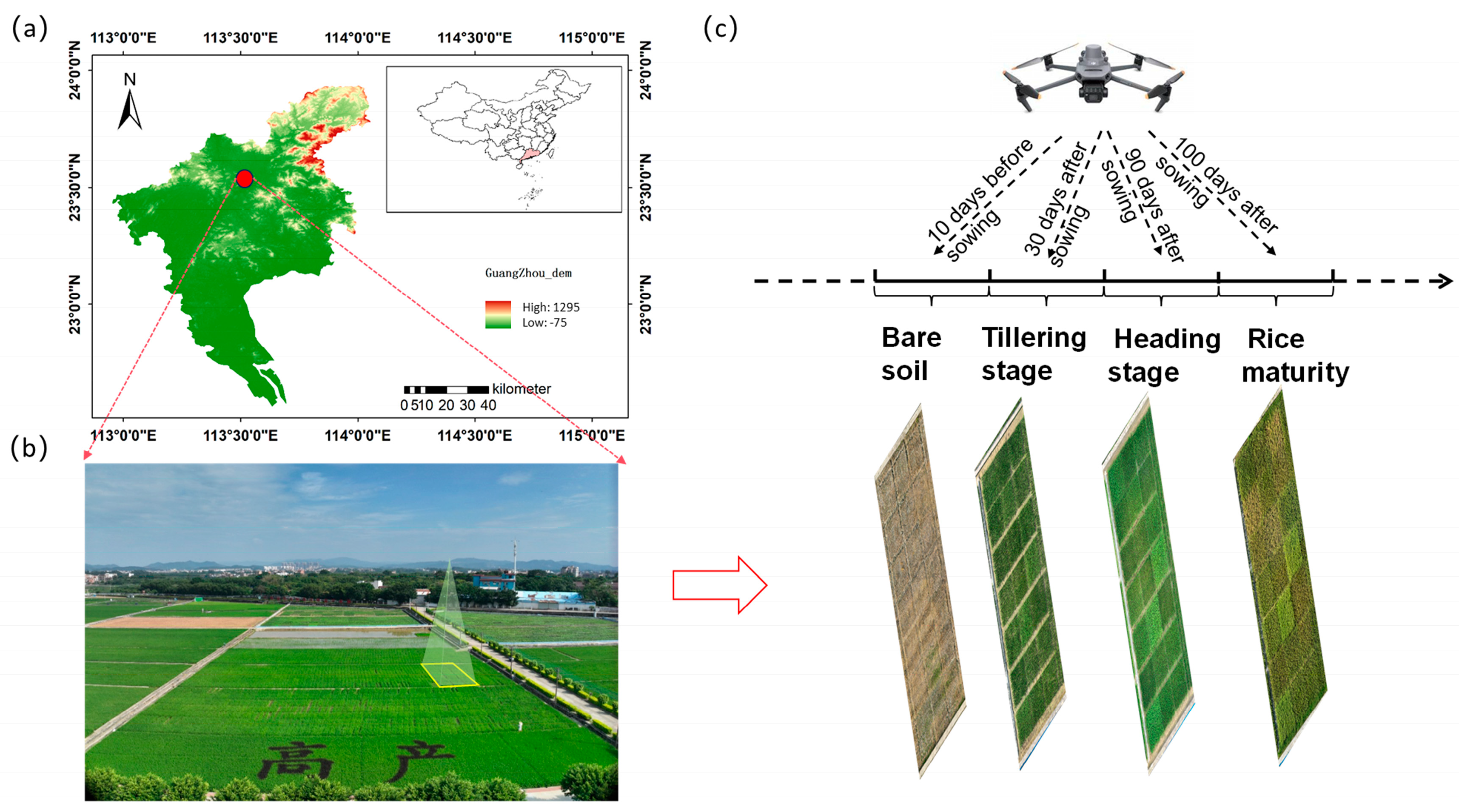
2.1.1. Overview of the Experimental Area and Soil Characteristics

This study was conducted in 2024 at the Baiyun Base of the Rice Research Institute, Baiyun District, Guangzhou City, Guangdong Province (113°25′ E, 23°23′ N, and 23.8 m above sea level) (Figure 1a). The experimental area has a subtropical monsoon climate, with abundant light and heat resources and precipitation. The average annual temperature is 21.5–22.2 °C, the yearly precipitation is about 1800 mm, and the annual precipitation days are about 150 days. The climatic conditions are suitable for rice growth. The experimental field is a modern, high-standard farmland. The results of the soil’s physical and chemical properties showed that the pH value was 6.11, the organic matter content was 27.87 g/kg, the total nitrogen content was 1.41 g/kg, the total phosphorus content was 1.03 g/kg, the total potassium content was 16.62 g/kg, and the available phosphorus content was 49.39 mg/kg. The available potassium content was 41.69 mg/kg. During the experiment, conventional water and fertilizer management measures were adopted to control the supply of water and nutrients strictly and ensure that the growth conditions of each experimental plot were consistent.

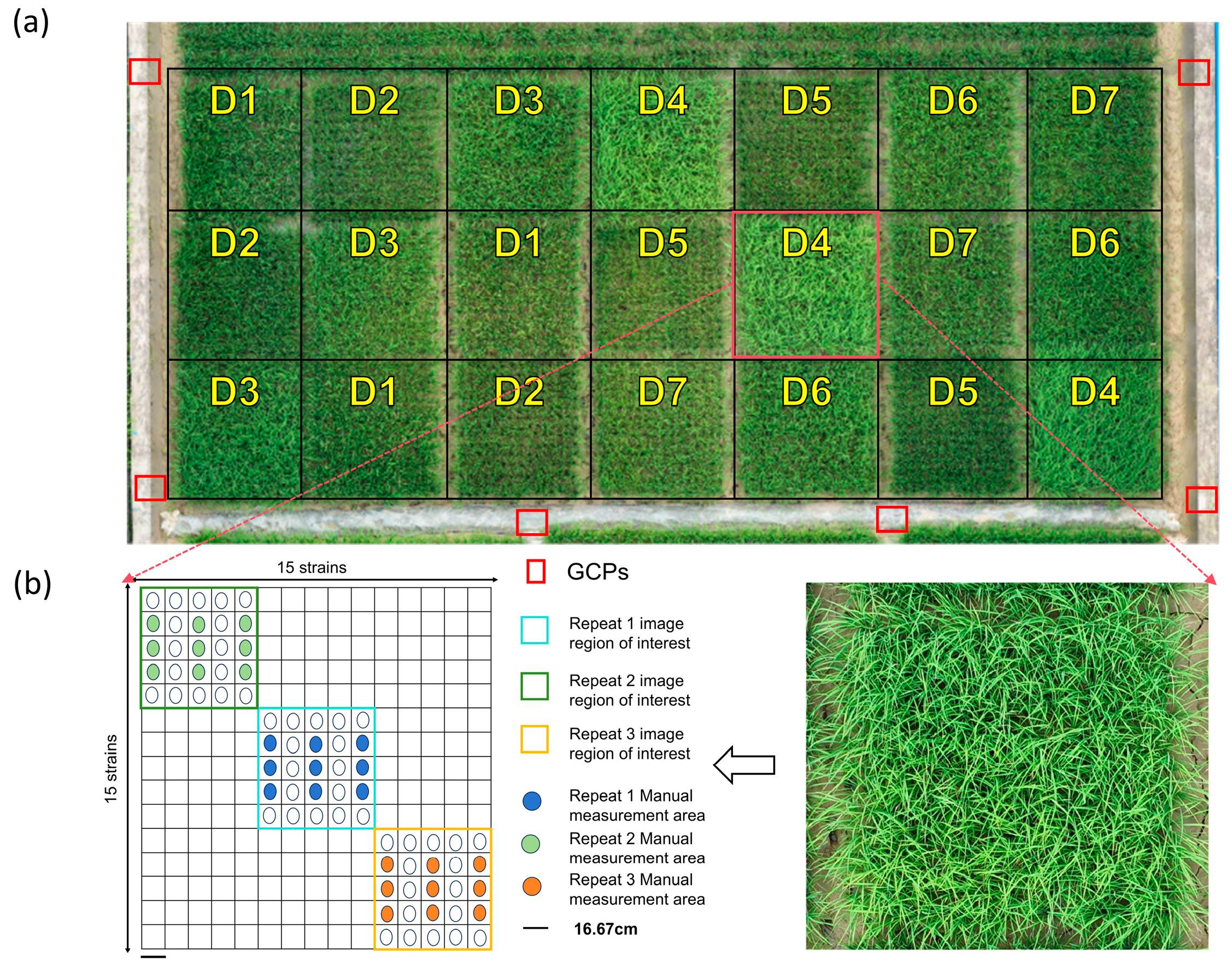
2.1.2. Test Materials and Layout

This study selected seven representative rice varieties (

Table 1. A variety of sources.

Serial Number	Rice Variety Name	Source	Rice Types	Rice Period
D1	Guangluai 4 hao	RRI GAAS *	Indica	106
D2	Guichao 2 hao	RRI GAAS *	Indica	111
D3	Huanghuazhan	RRI GAAS *	Indica	112
D4	Yuexiangzhan	RRI GAAS *	Indica	111
D5	Zhengkexinxuanmaio2hao	RRI GAAS *	Indica	104
D6	Yuenongsimiao	RRI GAAS *	Indica	110
D7	Yuehesimiao	RRI GAAS *	Indica	111

Note: RRI GAAS * express Rice Research Institute, Guangdong Academy of Agricultural Sciences.

), including Guangluai 4 hao, Guichao 2 hao, Huanghuazhan, Yuexiangzhan, Yuenongsimiao, Yuehesimiao, and Zengke Xinxuansimiao 2 hao. These varieties were provided by the Disease Resistance Breeding Research Group of the Rice Research Institute of Guangdong Academy of Agricultural Sciences. Yuexiangzhan is a representative variety with a high harvest index, and Zengke Xinxuansimiao 2 Hao is a representative variety with a low harvest index. This variety selection covering different harvest index ranges aims to provide a rich and differentiated data basis for a comprehensive and in-depth exploration of the rice harvest index prediction model. The experiment was sown on 20 March 2024, and field transplanting was completed on 7 April.

The experiment adopted a randomized block design, with three replicates for each variety (Figure 2a), to eliminate the systematic error of the field environment. The planting specifications of a single plot were 15 rows × 15 columns (a total of 225 plants), and the row–plant spacing was uniformly set to 16.7 cm × 16.7 cm to ensure the consistency of population density. To improve the representativeness and accuracy of data collection, each plot was divided into three sampling areas along the diagonal direction, and each sampling area contained 5 × 5 rice plants (25 plants). In each sampling area, the alternate row sampling method was adopted, and nine representative plants were selected for agronomic trait determination and harvest index investigation to ensure the randomness and representativeness of the samples.

2.2. Data Acquisition System

2.2.1. UAV Platform and Sensor Configuration

This study uses the DJI Mavic 3M drone system (Shenzhen DJI Innovations Technology, Shenzhen, China) as the main data collection platform (Figure 1b). The system integrates a high-precision RTK positioning module, which can obtain the camera imaging center coordinates with centimeter-level positioning accuracy in real time, providing an accurate spatial reference for later image processing. The system mainly consists of two parts: a visible light imaging system and a multispectral imaging system.

The visible light imaging system uses a 4/3 CMOS Hasselblad image sensor equipped with a DJI DL 24 mm lens, with an effective pixel count of 20 million (5280 × 3956 pixels). At a flight altitude of 12 m, an ultra-high ground resolution of 0.69 mm/pixel can be achieved, guaranteeing the accurate extraction of plant morphological characteristics. Images are stored in JPEG format on a high-speed SD card to ensure data acquisition continuity and reliability.

The multispectral imaging system uses a 5-megapixel (2592 × 1944 pixel) professional-grade multispectral camera, which includes four characteristic bands: green light (560 ± 16 nm), red light (650 ± 16 nm), red edge (730 ± 16 nm), and near-infrared (840 ± 26 nm) (

Table 2. Band parameters of sensors.

Band	Central Wavelength (nm)	Bandwidth (nm)
Green band	560	16
Red band	650	16
Red edge band	730	16
Near-infrared band	840	26

). The multispectral light intensity sensor integrated into the system can collect solar irradiance data in real time for image radiation correction, significantly improving spectral data in different periods.

2.2.2. Data Collection

A systematic data collection plan was developed for this study to ensure data quality and temporal continuity. Data were collected at four key periods during the rice growth period: first, bare soil images were collected before transplanting to build a digital terrain model (DTM), and then vegetation canopy information was collected at the tillering stage, heading stage, and maturity stage (Figure 1c). All aerial survey tasks were carried out under clear and windless weather conditions and were carried out during the period of 12:00–14:00 when the solar altitude angle was large and the light was stable to reduce shadow effects and ensure the reliability of spectral data.

The flight parameters were optimized: the flight altitude was maintained at 12 m, the flight speed was controlled at 1.0 m/s, and the shooting interval was set to 2 s. To ensure the image quality and 3D reconstruction accuracy, the forward overlap was set to 90%, and the lateral overlap was set to 80%. Eight ground control points (GCPs) were evenly arranged on the cement ridges around the experimental field, and their precise coordinates were obtained using an RTK surveying instrument for later image geometric correction and accuracy verification.

2.3. Data Processing and Analysis

2.3.1. Image Preprocessing

DJI Terra software (version 4.0.10) was used to preprocess the acquired raw images. First, the irradiance data recorded by the multispectral light intensity sensor carried by the drone was used to perform radiometric correction on the multispectral images to eliminate the influence of changes in light intensity at different times. The radiometric correction used standard reflectors with reflectivity of 25%, 50%, and 75% to establish a regression equation and convert digital values (DN values) into surface reflectivity.

The coordinates of the ground control points measured by RTK were combined with the image position information recorded during the flight of the UAV to ensure the geometric accuracy of the image. Subsequently, the region of interest (ROI) was polygonally delineated using ArcGIS 10.8 software (ArcGIS 10.8.0.12790) Environmental Systems Research Institute, Inc., Redlands, CA, USA) to extract image data from 25 rice plants in each experimental plot.

2.3.2. Feature Extraction and Calculation

Plant Height Information Extraction

Based on the Structure from Motion (SfM) technology, a digital surface model (DSM) was generated using high-resolution RGB images. The canopy height model (CHM) reflecting crop height information was obtained by subtracting the digital terrain model (DTM) obtained from the DSM during the bare soil period. To ensure the accuracy of height extraction, a 1 m × 1 m buffer was delineated around each area of interest with the RTK measurement point as the center, and the average plant height value in the area was extracted.

Spectral Feature Calculation

A series of spectral indices that can characterize crop physiological characteristics was calculated based on the corrected multispectral reflectance data.

Table 3. Vegetation index of different sensor data combinations.

Vegetation Index	Name	Sensor	Formula	References
NDVI	Normalized Difference Vegetation Index	MS	NDVI = (NIR − R)/(NIR + R)	[15]
RAVI	Ratio Vegetation Index	MS	RVI = (NIR/R)	[16]
NLI	Normalized Leaf Index	MS	NLI = (NIR2 − R)/(NIR2 + R)	[17]
NDRE	Normalized Difference Red Edge Index	MS	NDRE = (NIR − RE)/(NIR + RE)	[18]
OSAVI	Optimization of Soil Regulatory	MS	OSAVI = 1.16 × (NIR − R)/(NIR + R + 0.16)	[19]
TCARI	Transform Chlorophyll Absorption Index	MS	TCARI = 3 × (RE − R) − 0.2 × (RE − G) × (RE/R)	[20]
MCARI	Modified Chlorophyll Absorption Reflectance Index	MS	MCARI = (NIR − R − 0.2 × (RE − G)) × (RE/R)	[21]
GRVI	Green-Red Vegetation Index	MS	GRVI = (G − R)/(G + R)	[22]
MSRI	Modified Second Ratio Index	MS	MSRI = (√(NIR/R) − 1)/(√(NIR/R) + 1)	[23]
GCI	Green Chlorophyll Index	MS	GCI = NIR/G − 1	[23]
EVI2	Enhanced Vegetation Index	MS	EVI2 = 2.5 × (NIR − R)/(NIR + 2.4 × R + 1)	[24]
MNVI	Modified Normalized Vegetation Index	MS	MNVI = 1.5 × (NIR2 − R)/(NIR2 + R + 0.5)	[25]
RVI1	Ratio Vegetation Index	MS	RVI1 = NIR/R	[26]
RVI2	Ratio Vegetation Index	MS	RVI2 = NIR/G	[26]
TVI	Triangle Vegetation Index	MS	TVI= 60 × (NIR − G) − 100 × (R − G)	[25]
TO	Transform Soil-Adjusted Vegetation Index	MS	TO= 3 × ((REG − R)/(REG − G)) × (REG/R)/OSAVI	[27]
MTCI	MERIS Terrestrial Chlorophyll Index	MS	NDVI = (NIR − RE)/(RE − R)	[28]
SAVE	Soil-Adjusted Vegetation Index	MS	SAVI = (1 + L) (NIR − R)/(NIR + R + L)	[27]
CI	Chlorophyll Index	MS	CI = NIR/G − 1	[29]

mainly includes (Table 3) using the band operation module of ENVI software (ENVI 5.6 Exelis Visual Information Solutions Inc., Tysons Corne, VA, USA) to perform batch calculations of spectral indices and associating the calculation results with sample information to establish a complete spectral feature dataset.

2.4. Ground Data Collection

2.4.1. Determination of Agronomic Traits of Plant Height

In each experimental plot, nine representative plants were selected from three 5 × 5 plots according to the preset sampling plan for measurement (Figure 2b). Plant height was measured using a professional ruler, and marks were set at the measurement positions to ensure spatial correspondence with the drone remote sensing data. Plants with apparent growth abnormalities were marked in a timely manner and replaced with adjacent typical plants to ensure data quality.

2.4.2. Harvest Index Determination

At the rice maturity stage, the pre-marked samples were harvested by flat mowing. Nine plants were harvested in each of the three sample plots in each plot for a total of 63 plot samples. Threshing was carried out on-site, and the grains and straw were separated, bagged, and recorded. The grain samples were naturally dried to control the moisture content between 10% and 14%; the straw samples were treated by withering at 95 °C for 2 h and then drying at 60 °C for 3 days. After thoroughly drying the samples, they were weighed using an electronic balance with an accuracy of 0.01 g to calculate the harvest index.

2.5. Data Analysis and Modeling

2.5.1. Data Preprocessing

All the collected feature data are systematically preprocessed, including the following steps: Missing value processing: The nearest mean method is used to fill a small amount of missing data, and samples with a missing rate of more than 5% are eliminated. Outlier detection: The box plot method is used to identify outliers, and a decision on whether to exclude them is made after verification through field records. Data standardization: The Z-score standardization method is used to normalize the features of different dimensions: Z = (X − μ)/σ, where X is the original value, μ is the mean, and σ is the standard deviation.

2.5.2. Feature Selection and Optimization

A multi-level screening strategy was used for feature selection: The Pearson correlation coefficient between each feature and the harvest index was calculated, and the significantly correlated features (p < 0.05) were preliminarily screened.

Recursive feature elimination (RFE) was used to evaluate feature importance. Lasso regression was used for feature compression. XGBoost’s feature importance ranking was used for verification. Multicollinearity diagnosis was performed, and the variance inflation factor (VIF) was calculated. Features with VIF > 10 were removed to reduce redundancy between features.

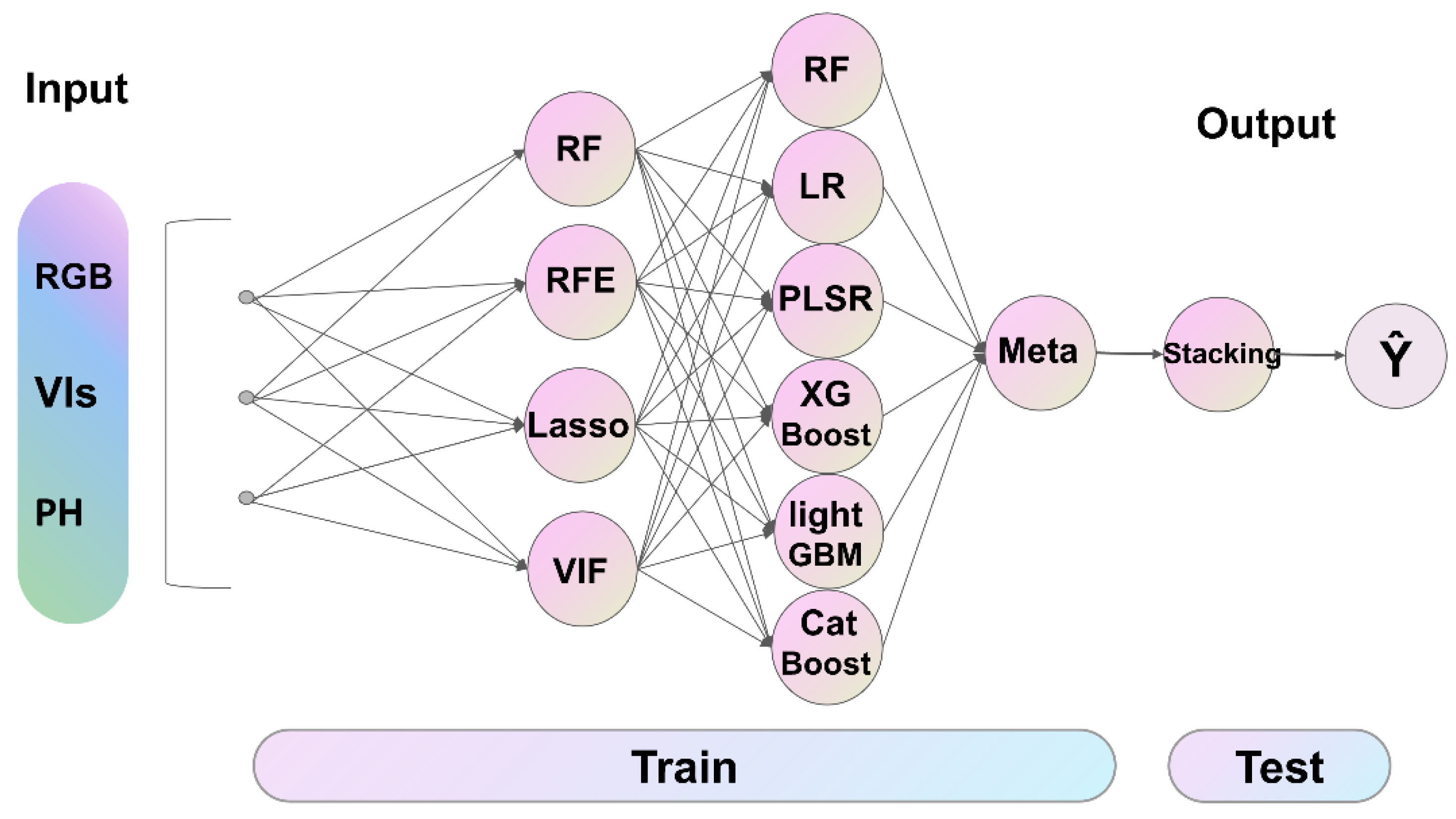
2.5.3. Model Construction and Integration

This study adopts a multi-level machine learning model architecture (Figure 3). Its basic model layer explicitly includes the following:

Random Forest: 500 decision trees were constructed, and the Gini coefficient was used as the splitting criterion. XGBoost: The learning rate was set to 0.1, and the maximum tree depth was 6. The mean square error was used as the objective function. LightGBM: The maximum number of leaves was limited to 31, the minimum amount of data was 20, and feature binning optimization was used. CatBoost: The number of iterations was set to 1000, and dynamic learning rate adjustment was used.

Using the Stacking integrated learning layer, the specific steps are as follows:

The dataset is divided into a training set and a test set in a ratio of 8:2. A 10-fold cross-validation method is used for the training set. Predictions are made on the validation set after the basic model is trained on the training set. The prediction results of each basic model are used as new features to construct a meta-learner. XGBoost, with the best performance, is used as the meta-learner to learn the optimal model combination weights.

2.5.4. Model Evaluation Methods

Evaluation of prediction accuracy: the coefficient of determination (R²) [30], which evaluates the degree to which the model explains the data variation (1); root mean square error (RMSE) [31], which measures the average deviation between the predicted value and the measured value (2).

$$R^2=1-{\displaystyle \frac{{\displaystyle \sum _{i=1}^n{(y_i-{\widehat{y}}_i)}^2}}{{\displaystyle \sum _{i=1}^n{(y_i-{\overline{y}}_i)}^2}}}$$

(1)

$$\mathrm{RMSE}=\sqrt{{\displaystyle \frac{1}{n}}{\displaystyle \sum _{i=1}^n{(y_i-{\widehat{y}}_i)}^2}}$$

(2)

Note: In these formulas, X$y_i$ represents the observed value (actual or measured dependent variable value), X${\widehat{y}}_i$ represents the predicted value obtained by using the model prediction, and X $\overline{y_i}$ represents the average of all observed values.

Model stability assessment: Use k-fold cross-validation to assess the generalization ability of the model; use the Bootstrap resampling method to assess the confidence interval of the model prediction; and use an independent test set to verify the performance of the model on new data.

Visual evaluation: Residual distribution diagram to test the randomness of prediction error; the scatter plot of predicted values and measured values to intuitively display the prediction accuracy; feature importance bar chart to analyze the contribution of each feature.

3. Results

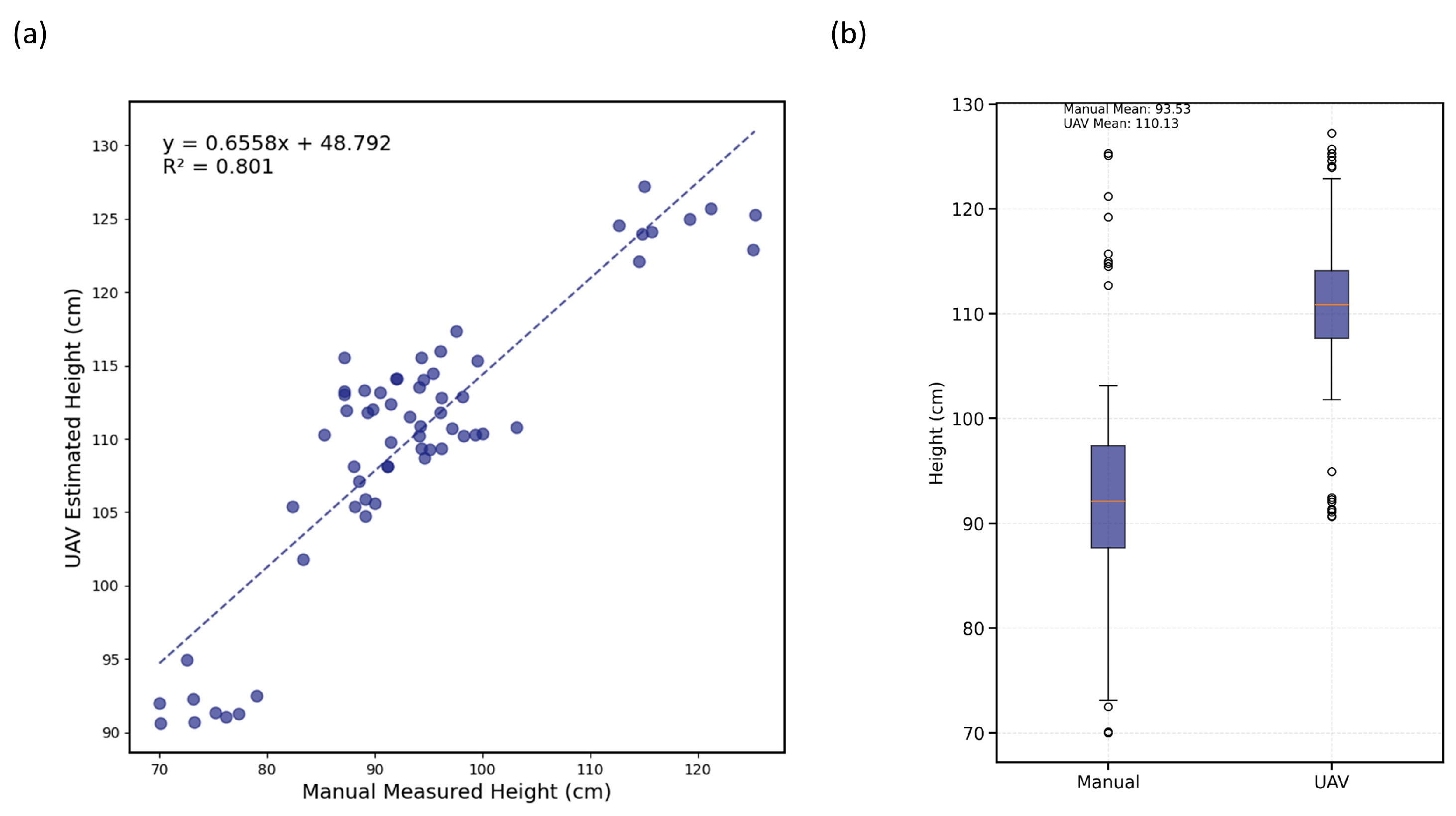
3.1. Verification of Plant Height Estimation Accuracy Using UAV Remote Sensing

Rice plant height is one of the important indicators for measuring aboveground biomass, which is closely related to the photosynthetic efficiency, dry matter accumulation, and harvest index (HI) of crops. Therefore, an accurate estimation of the height of the rice plant is of great significance when analyzing the prediction model of HI. In this study, UAV remote sensing technology combined with the digital surface model (DSM) reconstructed by Structure from Motion (SfM) was used to extract the rice canopy height (UAV_PH), and a systematic accuracy verification analysis was conducted with the traditional manually measured plant height (Manual_PH). The results are shown in the figure (Figure 4).

By establishing a linear regression model between the drone’s remote sensing height and the measured height, the regression equation was obtained: y = 1.2213x − 16.548, where y is the canopy height estimated by drone remote sensing, and x is the measured plant height. The coefficient of determination R² of the model is 0.801, indicating that the plant height data obtained by drone remote sensing can explain about 80.1% of the actual plant height variation.

This result proves that UAV remote sensing technology is highly reliable and accurate in rice plant height monitoring and is particularly suitable for large-scale, non-contact, rapid measurement. Further analysis found that the slope (1.22) in the regression equation is greater than 1. At the same time, the intercept (−16.55) is negative, indicating that the canopy height estimated by the UAV is slightly higher than the manual measurement value in the late stage of rice growth.

Generally, UAV remote sensing technology shows strong application potential in rice plant height estimation, especially in precision agriculture and high-throughput phenotyping monitoring. It provides reliable basic data for further analysis of rice biomass and HI prediction.

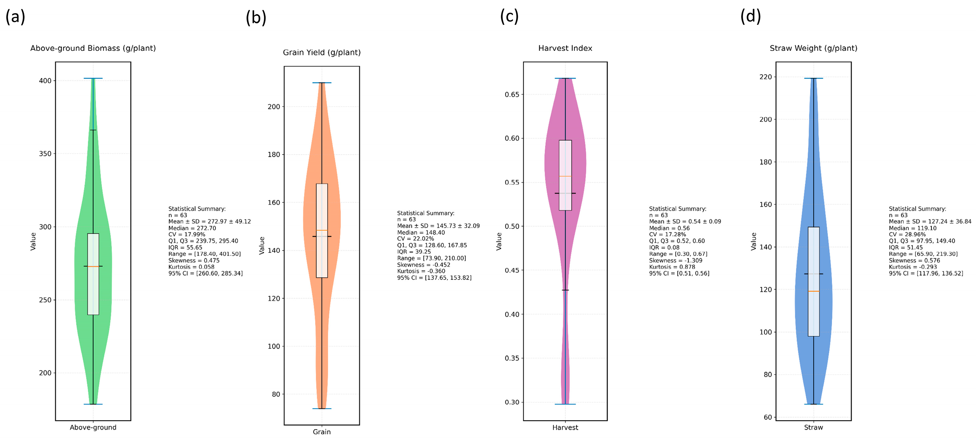
3.2. Analysis of Ground Data Harvest Index Verification

This study systematically analyzed the key agronomic traits of rice field trials, aiming to provide reliable data support for constructing a harvest index prediction model based on UAV remote sensing. The results showed that the harvest index (HI) of the tested rice population showed an ideal normal distribution, with an average value of 0.54 ± 0.09, a coefficient of variation of 17.28%, and a distribution range of [0.30, 0.67], which was highly consistent with the typical harvest index range of rice reported in previous studies (Figure 5). The data showed a slightly negatively skewed distribution (skewness = −1.30), and the kurtosis value (0.878) was close to the standard normal distribution, with a 95% confidence interval of [0.51, 0.56], which fully confirmed the representativeness of the sample and the reliability of data collection. Among the essential agronomic traits required for model construction, straw weight (SW), aboveground biomass (AGB), and grain yield (GY) all showed an ideal range of variation. This variation characteristic reflects the natural conditions of the field experiment and provides solid data support for establishing the quantitative relationship between UAV remote sensing parameters and harvest index.

From the technical perspective of modeling, the agronomic trait data obtained in this study have three significant advantages: first, the approximately typical distribution characteristics of the harvest index provide an ideal data structure for the construction of a regression model; second, the moderate coefficient of variation reflects the inherent stability of the data, which will effectively improve the predictive reliability of the model; finally, the complete data distribution range provides sufficient sample representativeness for the calibration and verification of the model.

In addition, the distribution characteristics of agronomic trait data also reveal the inherent laws of rice growth and development. The negatively skewed distribution of the harvest index indicates that under standard cultivation conditions, rice tends to maintain a relatively stable biomass distribution pattern. These findings not only provide reliable ground verification data for UAV remote sensing estimation of rice harvest index, but their statistical characteristics also support the feasibility of predictive model construction from multiple dimensions, laying an important theoretical and data foundation for the development of remote-sensing-based rapid diagnosis methods for rice harvest index but also provide new technical ideas for crop phenotyping research.

3.3. Evaluation of Machine Learning Model Prediction Performance

Based on the screened significant spectral feature variables (MTCI, TCARI, GRVI, and TO), this study constructed a multi-level machine learning model system, including random forest (RF), linear regression (LR), partial least squares regression (PLSR), XGBoost, LightGBM, CatBoost, and Stacking ensemble learning models. A 10-fold cross-validation method was used to train and evaluate the performance of all models. The evaluation indicators included the coefficient of determination (R²), root mean square error (RMSE), and mean square error (MSE).

The results show that the Stacking ensemble learning model exhibits the best prediction performance (Figure 6), with a coefficient of determination (R²) of 0.88, a root mean square error (RMSE) of 0.18, and a mean square error (MSE) of only 0.03. The XGBoost and LightGBM models also showed good predictive capabilities, with XGBoost’s R² of 0.81 (RMSE = 0.22, MSE = 0.05) and LightGBM ‘s R² of 0.77 (RMSE = 0.25, MSE = 0.062). Traditional machine learning models such as random forests (R² = 0.73) and support vector machines (R² = 0.65) performed poorly.

The Stacking model performed best (

Table 4. The accuracy calculation results of each model, R², and RMSE.

MODEL	R2	RMSE
Random Forest	0.79	0.0251
Linear Regression	0.82	0.0235
PLSR	0.81	0.0240
XGBoost	0.78	0.0253
LightGBM	0.81	0.0244
CatBoost	0.77	0.0256
Stacking	0.88	0.0189

): the coefficient of determination reached 0.88, and the root mean square error (RMSE) was 0.0189, which was significantly better than other single models. The model significantly improves the prediction accuracy by integrating the advantages of multiple base learners (such as XGBoost and LightGBM) and demonstrates a strong ability to fit complex nonlinear relationships. The gradient boosting model XGBoost is 0.81 (RMSE = 0.024), and the R² of LightGBM is 0.77 (RMSE = 0.025). The gradient boosting method performed well, verifying its advantages in processing high-dimensional complex data.

Traditional models performed poorly: the random forest model had an R² of 0.79, while the linear regression model had an R² of 0.82. Although these models have specific predictive capabilities, they cannot capture the nonlinear relationship between complex spectral features and HI.

From the error distribution diagram (Figure 6), the residual distribution of the Stacking model is the most concentrated, indicating that the deviation between its predicted value and the actual value is the smallest. In comparison, the residual distribution of random forest and linear regression is more scattered, and the prediction performance is relatively low.

The main reason for the excellent performance of the Stacking model lies in its unique model integration advantage, which can effectively reduce the deviation of a single model by combining the prediction results of multiple base learners and making full use of the complementarity of different models in feature learning. At the same time, the model has a strong modeling ability for the interaction of multi-source remote sensing features and shows strong robustness when processing high-dimensional features. In particular, the Stacking ensemble learning model has significant application potential in predicting the rice harvest index, providing reliable technical support for high-throughput phenotypic screening in the rice breeding process and an important decision-making basis for precision agricultural management.

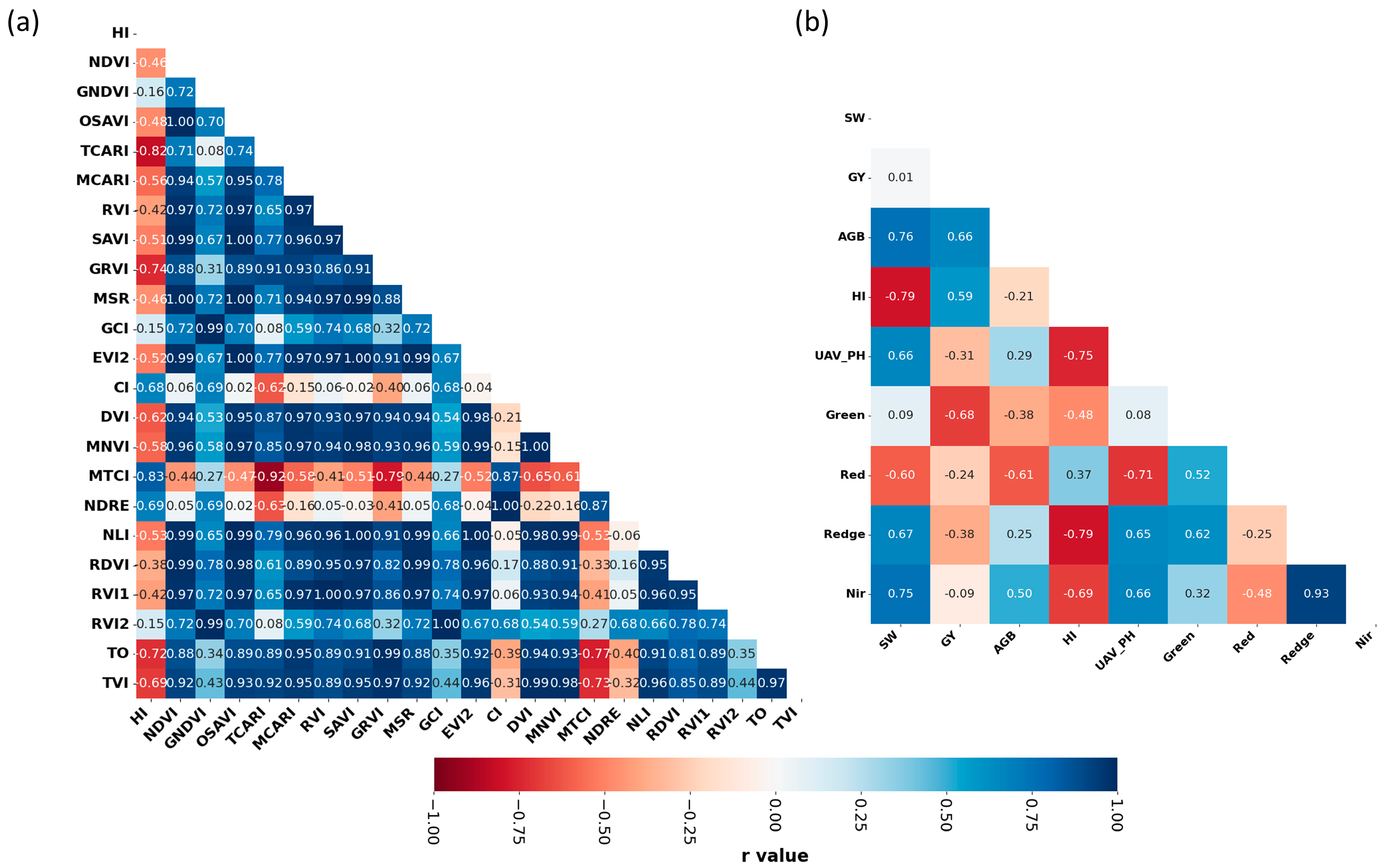
3.4. Correlation Analysis Between the Spectral Index and Harvest Index

Pearson correlation analysis on their correlation with HI (Figure 7a). The results are shown in

Table 5. Strongly correlated spectral index.

Spectral Index	Correlation Coefficient (r)	Significant (p)	Degree of Relevance
MTCI	0.83	<0.01	Strong positive correlation
TCARI	−0.82	<0.01	Strong negative correlation
TO	−0.72	<0.01	Significant negative correlation
GRVI	−0.74	<0.01	Significant negative correlation
NDRE	0.69	<0.01	Significant positive correlation
CI	0.68	<0.01	Significant positive correlation
TVI	−0.69	<0.01	Significant negative correlation

Note: |r| ≥ 0.8 is a strong correlation; 0.6 ≤ |r| < 0.8 is a significant correlation.

Based on Pearson correlation analysis, seven key spectral indices were found to be significantly correlated with HI (Table 5). MTCI (Meris Terrestrial Chlorophyll Index) showed a significant positive correlation with HI (r = 0.83). As an important indicator reflecting the chlorophyll content of the canopy, this relevant characteristic of MTCI indicates that a higher photosynthetic substance accumulation capacity helps to improve the efficiency of dry matter transport to grains. This finding provides a reliable spectral indicator for assessing rice yield potential.

TCARI (Transformed Chlorophyll Absorption in Reflectance Index) was significantly negatively correlated with HI (r = −0.82). TCARI mainly reflects the relationship between canopy red light absorption and leaf structure. Its negative correlation indicates that if crops accumulate too much leaf biomass during the vegetative growth stage, photosynthetic products may not be effectively distributed to grains, thereby reducing HI.

GRVI (Green–Red Vegetation Index) and TO index were significantly negatively correlated with HI (r = −0.74 and r = −0.72), respectively. Both reflect the canopy’s green structure and the red light reflectance characteristics. Too high GRVI and TO values usually mean that the crop’s vegetative growth is too vigorous, and a high proportion of photosynthetic products are allocated to non-harvested parts (such as stems and leaves), inhibiting grain yield formation.

4. Discussion

4.1. Importance of Spectral Index to Harvest Index Prediction Model

HI (harvest index) measures the efficiency of crops in converting dry matter into grains. A high HI means that the crop can efficiently convert its accumulated biomass into harvestable grains instead of wasting it on non-harvestable parts (such as stems and leaves) [32]. The chlorophyll content of a plant is closely related to its photosynthetic efficiency. The red edge band and the near-infrared band are susceptible to the reflectance and absorption of chlorophyll and can help evaluate the photosynthetic efficiency of crops [33]. The red edge band is between 700 and 800 nm and is an important part of the plant spectrum. It has a strong sensitivity to chlorophyll absorption. This band is susceptible to plant photosynthesis, chlorophyll content, and plant health. Since chlorophyll absorbs red and blue light and reflects less to the red edge band, the red edge band has become an effective indicator for measuring plant health and photosynthesis efficiency. The near-infrared band (NIR) is between 750 and 1300 nm and is one of the strongest bands reflected by plants. Healthy plant leaves can reflect more near-infrared light, so it is often used to estimate crop biomass and water status [34]. The red edge band and near-infrared band are susceptible to crop biomass accumulation and can effectively reflect information such as crop chlorophyll content, biomass, and water status [14,35,36]. These spectral indices with high correlation with HI (such as TCARI, GRVI, and TO index) all use a combination of red-edge band and near-infrared band and also directly reflect the relationship between rice photosynthesis, chlorophyll content, and biomass accumulation (Figure 7b).

During the growth of crops such as rice, the crop’s biomass (mainly the accumulation of stems and leaves) and the organic matter produced by photosynthesis are dynamically distributed [32]. At the heading stage, the growth of the crop is still focused on the development of stems and leaves, and the dry matter produced by photosynthesis has not yet been fully converted into grains. At the maturity stage, more of the photosynthetic products of the crop are converted into grains, achieving the highest biomass conversion efficiency.

Photosynthesis efficiency is a key factor in determining crop dry matter accumulation and conversion efficiency [37]. At the heading stage, rice’s growth mainly depends on the development of stems and leaves. Vegetation indices (such as NDVI, MTCI, etc.) primarily reflect the growth status of the green part, while the photosynthetic products of these parts are not all converted into grains [3]. Therefore, the current correlation between the vegetation index and HI is weak.

During the maturity period, the efficiency of converting rice photosynthetic products into grains reaches its highest level, and the chlorophyll content and photosynthesis intensity gradually stabilize [38]. At this time, the vegetation index can effectively reflect the physiological state of the crop and the final distribution of biomass, especially the part converted into grains. Therefore, the vegetation index strongly correlates with the HI during the maturity period.

4.2. Small Sample Learning and Feature Parameter Optimization

This study revealed the differences in the contribution of different features to the prediction of rice harvest index through SHAP value analysis, which is consistent with the results of previous studies [39]. Initial analysis showed that in the complete feature set, the GRVI vegetation index at the heading stage, pH at maturity, and GRVI vegetation index at maturity showed the most significant prediction contributions. After multi-level feature screening, the key features were further confirmed: the SHAP value of maturity CI reached −0.12, showing the most substantial negative contribution; maturity MTCI and maturity PH also showed significant predictive ability, with SHAP values of approximately −0.06 and −0.02, respectively. This significant stratification of feature importance verifies the necessity and effectiveness of our multi-level feature screening strategy [40].

The multi-level feature screening strategy adopted in this study improved the model prediction accuracy (R² = 0.88). This systematic feature engineering method is significantly superior to the traditional single-feature selection method [41]. First, the initial screening based on Pearson correlation analysis (p < 0.05) provided a reliable statistical basis for feature selection. Secondly, the combined application of recursive feature elimination (RFE) and Lasso regression realizes the sparse representation of features and effectively reduces the complexity of the model. In particular, through the variance inflation factor (VIF) diagnosis (VIF > 10 as the threshold), features with unique predictive contributions, such as CI and MTCI, were successfully identified and retained, which significantly improved the stability and interpretability of the model.

This optimized feature subset forms a good synergistic effect with the Stacking ensemble learning framework [42]. As shown in the SHAP diagram, in the filtered feature set, the distribution of different feature values is more discrete, indicating that these features can provide the model with more discriminative prediction information. In particular, the two key features of maturity CI and MTCI, their SHAP value distributions, show prominent hierarchical characteristics, indicating that they can effectively capture the essential relationship between rice physiological characteristics and harvest index [43]. This high-quality feature input enables the basic model to more accurately learn the complementary relationship between features, thereby producing more reliable prediction results in the ensemble learning stage [13].

It is worth noting that the SHAP analysis results after feature screening show a more apparent hierarchy of feature importance, which not only verifies the effectiveness of the feature selection strategy but also improves the interpretability of the model. For example, the significant contributions of CI and MTCI indicate that canopy structure and chlorophyll content are key factors affecting the rice harvest index. This finding is consistent with previous research results and provides an important theoretical basis for precision agricultural management [44] (Figure 8).

However, even in the optimized feature set, the SHAP values of some features still overlap, suggesting that we consider adopting more sophisticated feature selection strategies in future research. For example, we can introduce a feature weight adaptation method based on the attention mechanism or explore deep feature extraction technology to improve the model’s prediction performance further [45]. At the same time, considering the actual needs of agricultural production, we can also explore how to simplify further the feature set while maintaining the model performance to improve the model’s efficiency and operability in practical applications [8,41].

4.3. Research Limitations and Future Directions

Although the rice harvest index prediction method proposed herein demonstrates high predictive accuracy, it has several limitations. Firstly, the acquisition of remote sensing data is inherently subject to constraints imposed by meteorological conditions and sensor resolution capabilities, which can potentially impact data integrity and temporal consistency. Secondly, concerning model generalizability, the current study incorporated seven rice varieties exhibiting significant genetic diversity (encompassing Indica and Japonica subspecies and representative high, medium, and low HI lines) and utilized a randomized block design with triplicate replication—aiming to systematically analyze the genetic and phenotypic interplay between canopy characteristics and HI—acknowledging the substantial heritability of key agronomic traits in rice [46], which partially mitigates the confounding influence of the environment within this single setting. Nevertheless, the foundational dataset was derived exclusively from a single geographical locale (Baiyun District, Guangzhou, China) during one specific growing season (2024 early rice). This restricted spatio-temporal scope inherently limits the validated generalizability of the current model across diverse agro-ecological contexts (encompassing varying climates, soil types, management practices, and phenological cycles).

Consequently, future research should prioritize the enhancement of the model’s generalization capacity and robustness. A principal objective involves substantially expanding the spatio-temporal and environmental diversity of the data sampling. Subsequent studies are planned to broaden the experimental scope through multi-locational and multi-seasonal trials encompassing diverse climatic zones (e.g., including tropical-subtropical transition regions), multiple growing seasons (e.g., incorporating early and late rice cycles), and a range of agronomic management practices (e.g., varying fertilization and irrigation regimes). Such expansion is anticipated not only to augment the dataset size but, more crucially, to facilitate the rigorous evaluation and enhancement of the model’s adaptability to variations in geographical provenance, climatic conditions, and cultivation systems, thereby bolstering its broader applicability.

Furthermore, advancements on the technological front, such as the incorporation of higher-resolution hyperspectral data, hold significant promise for capturing more nuanced spectral information. Integrating these data with sophisticated deep learning algorithms (e.g., CNNs and transformers) may potentially unlock more intricate patterns, thereby offering expanded scope for enhancing predictive accuracy. Concurrently, the exploration and development of multi-scale feature extraction frameworks, designed to synergistically integrate remote sensing information across diverse spatial and temporal resolutions, constitute another pertinent avenue for achieving a more holistic characterization of crop physiological status.

5. Conclusions

This study investigated the application of UAV remote sensing technology for predicting the crop harvest index (HI), overcoming the traditional constraint that HI could only be measured post-harvest. By extracting spectral features, including digital surface elevation and vegetation indices (e.g., TCARI, GRVI, MTCI, and TO) from UAV imagery, significant correlations were established between these variables and HI as well as aboveground biomass. During model development, multiple machine learning algorithms were systematically evaluated, and the Stacking ensemble learning model achieved superior predictive accuracy (R² = 0.88), significantly outperforming single-algorithm approaches. The integration of multi-source remote sensing features with multi-algorithm optimization enhanced prediction robustness, which underscored the practical potential of combining UAV-derived data with machine learning for agricultural remote sensing. This work provided a technical framework for screening crop varieties with high HI potential based on vegetation indices and offered actionable insights for precision agricultural practices, including fertilization, irrigation, and yield forecasting. These advancements contributed to the foundational knowledge required for intelligent and sustainable agricultural systems.

References

1. Khush, G.S. What it will take to Feed 5.0 Billion Rice consumers in 2030. Plant Mol. Biol. 2005, 59, 1–6. [Google Scholar] [CrossRef] [PubMed]
2. Wang, S.; Zhang, L.; Liu, W.; Wang, X.; Wu, H.; Chen, H.; Chen, T.; Lu, Z.; He, X. Two-year QTL dissecting of high harvest index and related traits in a novel rice variety Yuenongsimaio. Curr. Plant Biol. 2025, 42, 100475. [Google Scholar] [CrossRef]
3. Peng, S.; Khush, G.; Cassman, K. Evolution of the new plant ideotype for increased yield potential. In Proceedings of the Breaking the Yield Barrier: Proceedings of the Workshop on Rice Yield Potential in Favourable Environments, Los Banos, Philippines, 29 November–4 December 1994; pp. 5–20. [Google Scholar]
4. He, X.; Liao, Y.; Chen, Z.; Chen, S. Study on photosynthate’s transport and distribution characteristics in Yuexiangzhan, a rice variety with a high harvest index. J. South China Agric. Univ. 2000, 3, 5–8. [Google Scholar]
5. Xue, J.; Su, B. Significant remote sensing vegetation indices: A review of developments and applications. J. Sens. 2017, 2017, 1353691. [Google Scholar] [CrossRef]
6. Bendig, J.; Bolten, A.; Bennertz, S.; Broscheit, J.; Eichfuss, S.; Bareth, G. Estimating biomass of barley using crop surface models (CSMs) derived from UAV-based RGB imaging. Remote Sens. 2014, 6, 10395–10412. [Google Scholar] [CrossRef]
7. Maimaitijiang, M.; Sagan, V.; Sidike, P.; Maimaitiyiming, M.; Hartling, S.; Peterson, K.T.; Maw, M.J.; Shakoor, N.; Mockler, T.; Fritschi, F.; et al. Vegetation index weighted canopy volume model (CVMVI) for soybean biomass estimation from unmanned aerial system-based RGB imagery. ISPRS J. Photogramm. Remote Sens. 2019, 151, 27–41. [Google Scholar] [CrossRef]
8. Chlingaryan, A.; Sukkarieh, S.; Whelan, B. Machine learning approaches for crop yield prediction and nitrogen status estimation in precision agriculture: A review. Comput. Electron. Agric. 2018, 151, 61–69. [Google Scholar] [CrossRef]
9. İrik, H.A.; Ropelewska, E.; Çetin, N. Using spectral vegetation indices and machine learning models for predicting the yield of sugar beet (Beta vulgaris L.) under different irrigation treatments. Comput. Electron. Agric. 2024, 221, 109019. [Google Scholar] [CrossRef]
10. Kamilaris, A.; Prenafeta-Boldú, F.X. Deep learning in agriculture: A survey. Comput. Electron. Agric. 2018, 147, 70–90. [Google Scholar] [CrossRef]
11. Fass, E.; Shlomi, E.; Ziv, C.; Glickman, O.; Helman, D. Machine learning models based on hyperspectral imaging for pre-harvest tomato fruit quality monitoring. Comput. Electron. Agric. 2025, 229, 109788. [Google Scholar] [CrossRef]
12. Zhou, Z.-H. Ensemble Methods: Foundations and Algorithms; CRC Press: Boca Raton, FL, USA, 2012. [Google Scholar]
13. Zhou, X.; Zheng, H.; Xu, X.; He, J.; Ge, X.; Yao, X.; Cheng, T.; Zhu, Y.; Cao, W.; Tian, Y.; et al. Predicting grain yield in rice using multi-temporal vegetation indices from UAV-based multispectral and digital imagery. ISPRS J. Photogramm. Remote Sens. 2017, 130, 246–255. [Google Scholar] [CrossRef]
14. Jay, S.; Baret, F.; Dutartre, D.; Malatesta, G.; Héno, S.; Comar, A.; Weiss, M.; Maupas, F. Exploiting the centimeter resolution of UAV multispectral imagery to improve remote-sensing estimates of canopy structure and biochemistry in sugar beet crops. Remote Sens. Environ. 2019, 231, 110898. [Google Scholar] [CrossRef]
15. Rouse, J.W., Jr.; Haas, R.H.; Deering, D.W.; Schell, J.A.; Harlan, J.C. Monitoring the Vernal Advancement and Retrogradation (Green Wave Effect) of Natural Vegetation. In Earth Resources And Remote Sensing; NASA/GSFCT Type III Final Report. No. E75-10354; Texas A&M University: College Station, TX, USA, 1974. [Google Scholar]
16. Pearson, R.L.; Miller, L.D. Remote mapping of standing crop biomass for estimation of the productivity of the shortgrass prairie, Pawnee National Grasslands, Colorado. In Proceedings of the Eighth International Symposium on Remote Sensing of Environment, Ann Arbor, MI, USA, 2–6 October 1972. [Google Scholar]
17. Vescovo, L.; Gianelle, D. Using the MIR bands in vegetation indices for the estimation of grassland biophysical parameters from satellite remote sensing in the Alps region of Trentino (Italy). Adv. Space Res. 2008, 41, 1764–1772. [Google Scholar] [CrossRef]
18. Ju, C.-H.; Tian, Y.-C.; Yao, X.; Cao, W.-X.; Zhu, Y.; Hannaway, D. Estimating Leaf Chlorophyll Content Using Red Edge Parameters. Pedosphere 2010, 20, 633–644. [Google Scholar] [CrossRef]
19. Rondeaux, G.; Steven, M.; Baret, F. Optimization of soil-adjusted vegetation indices. Remote Sens. Environ. 1996, 55, 95–107. [Google Scholar] [CrossRef]
20. Haboudane, D.; Miller, J.R.; Pattey, E.; Zarco-Tejada, P.J.; Strachan, I.B. Hyperspectral vegetation indices and novel algorithms for predicting green LAI of crop canopies: Modeling and validation in the context of precision agriculture. Remote Sens. Environ. 2004, 90, 337–352. [Google Scholar] [CrossRef]
21. Im, J.; Jensen, J.R. Hyperspectral Remote Sensing of Vegetation. Geogr. Compass 2008, 2, 1943–1961. [Google Scholar] [CrossRef]
22. Chen, J.M.; Cihlar, J. Retrieving leaf area index of boreal conifer forests using Landsat TM images. Remote Sens. Environ. 1996, 55, 153–162. [Google Scholar] [CrossRef]
23. Zhang, X.; Friedl, M.A.; Schaaf, C.B.; Strahler, A.H.; Hodges, J.C.F.; Gao, F.; Reed, B.C.; Huete, A. Monitoring vegetation phenology using MODIS. Remote Sens. Environ. 2003, 84, 471–475. [Google Scholar] [CrossRef]
24. Jhorar, R.K.; Smit, A.; Roest, C.W.J. Assessment of alternative water management options for irrigated agriculture. Agric. Water Manag. 2009, 96, 975–981. [Google Scholar] [CrossRef]
25. Rouse, J.W.; Haas, R.H.; Schell, J.A.; Deering, D.W. Monitoring vegetation systems in the Great Plains with ERTS. NASA Spec. Publ. 1974, 351, 309. [Google Scholar]
26. Daughtry, C.S.T.; Walthall, C.L.; Kim, M.S.; De Colstoun, E.B.; McMurtrey Iii, J.E. Estimating corn leaf chlorophyll concentration from leaf and canopy reflectance. Remote Sens. Environ. 2000, 74, 229–239. [Google Scholar] [CrossRef]
27. Huete, A.R. A soil-adjusted vegetation index (SAVI). Remote Sens. Environ. 1988, 25, 295–309. [Google Scholar] [CrossRef]
28. Dash, J.; Curran, P.J. The MERIS terrestrial chlorophyll index. Int. J. Remote Sens. 2004, 25, 5403–5413. [Google Scholar] [CrossRef]
29. Gitelson, A.A.; Merzlyak, M.N.J. Remote estimation of chlorophyll content in higher plant leaves. Int. J. Remote Sens. 1997, 18, 2691–2697. [Google Scholar] [CrossRef]
30. Kvålseth, T.O. Cautionary Note about R 2. Am. Stat. 1985, 39, 279–285. [Google Scholar] [CrossRef]
31. Chai, T.; Draxler, R.R.J. Root mean square error (RMSE) or mean absolute error (MAE)?–Arguments against avoiding RMSE in the literature. Geosci. Model Dev. 2014, 7, 1247–1250. [Google Scholar] [CrossRef]
32. Yang, J.; Zhang, J.J. Grain filling of cereals under soil drying. New Phytol. 2006, 169, 223–236. [Google Scholar] [CrossRef]
33. Gitelson, A.; Merzlyak, M.N. Spectral Reflectance Changes Associated with Autumn Senescence of Aesculus hippocastanum L. and Acer platanoides L. Leaves. Spectral Features and Relation to Chlorophyll Estimation. J. Plant Physiol. 1994, 143, 286–292. [Google Scholar] [CrossRef]
34. Hansen, P.; Schjoerring, J.J. Reflectance measurement of canopy biomass and nitrogen status in wheat crops using normalized difference vegetation indices and partial least squares regression. Remote Sens. Environ. 2003, 86, 542–553. [Google Scholar] [CrossRef]
35. Horler, D.; Dockray, M.; Barber, J.J. The red edge of plant leaf reflectance. Int. J. Remote Sens. 1983, 4, 273–288. [Google Scholar] [CrossRef]
36. Cao, Q.; Miao, Y.; Wang, H.; Huang, S.; Cheng, S.; Khosla, R.; Jiang, R. Non-destructive estimation of rice plant nitrogen status with Crop Circle multispectral active canopy sensor. Field Crops Res. 2013, 154, 133–144. [Google Scholar] [CrossRef]
37. Yoshida, S.; Cock, J.; Parao, F. Physiological Aspects of High Yields. Annu. Rev. Plant Physiol. 1972, 23, 437–464. [Google Scholar] [CrossRef]
38. Zhang, H.; Tan, G.; Yang, L.; Yang, J.; Zhang, J.; Zhao, B.J. Hormones in the grains and roots in relation to post-anthesis development of inferior and superior spikelets in japonica/indica hybrid rice. Plant Physiol. Biochem. 2009, 47, 195–204. [Google Scholar] [CrossRef]
39. Lundberg, S.M.; Lee, S.I. A unified approach to interpreting model predictions. Adv. Neural Inf. Process. Syst. 2017, 30, 4768–4777. [Google Scholar]
40. Ma, L.; Fu, T.; Blaschke, T.; Li, M.; Tiede, D.; Zhou, Z.; Ma, X.; Chen, D.J. Evaluation of feature selection methods for object-based land cover mapping of unmanned aerial vehicle imagery using random forest and support vector machine classifiers. ISPRS Int. J. Geo-Inf. 2017, 6, 51. [Google Scholar] [CrossRef]
41. Cai, Y.; Guan, K.; Peng, J.; Wang, S.; Seifert, C.; Wardlow, B.; Li, Z.J. A high-performance and in-season classification system of field-level crop types using time-series Landsat data and a machine learning approach. Remote Sens. Environ. 2018, 210, 35–47. [Google Scholar] [CrossRef]
42. Shahhosseini, M.; Hu, G.; Archontoulis, S.V.J. Forecasting corn yield with machine learning ensembles. Front. Plant Sci. 2020, 11, 1120. [Google Scholar] [CrossRef]
43. Gitelson, A.A.; Peng, Y.; Huemmrich, K.F.J. Relationship between fraction of radiation absorbed by photosynthesizing maize and soybean canopies and NDVI from remotely sensed data taken at close range and from MODIS 250 m resolution data. Remote Sens. Environ. 2014, 147, 108–120. [Google Scholar] [CrossRef]
44. Zhou, X.; Zhu, X.; Dong, Z.; Guo, W. Estimation of biomass in wheat using random forest regression algorithm and remote sensing data. Crop J. 2016, 4, 212–219. [Google Scholar]
45. Zhang, L.; Zhang, L.; Du, B. Deep learning for remote sensing data: A technical tutorial on the state of the art. IEEE Geosci. Remote Sens. Mag. 2016, 4, 22–40. [Google Scholar] [CrossRef]
46. Huang, X.; Wei, X.; Sang, T.; Zhao, Q.; Feng, Q.; Zhao, Y.; Li, L.C.; Zhu, Z.C.; Lu, L.T.; Zhang, Z. Genome-wide association studies of 14 agronomic traits in rice landraces. Nat. Genet. 2010, 42, 961–967. [Google Scholar] [CrossRef]
Figure 1. (a) shows the experimental research area; (b) shows the experiment at the high-standard farmland research base; (c) shows the four periods of image acquisition (bare soil, rice tillering stage, rice heading stage, and rice maturity stage).
Agriculture 15 00971 g001
Figure 2. (a) shows the random distribution of varieties in the field; (b) shows the planting specifications of a single plot. The dots represent the manual sampling locations, and the squares represent the locations of interest for image acquisition.
Agriculture 15 00971 g002
Figure 3. This figure shows the framework diagram of the model.
Agriculture 15 00971 g003
Figure 4. This figure shows the comparison of the accuracy of manual measurement of rice height and UAV measurement of height. (a) shows the scatter plot of plant height measured manually and by drone; (b) shows the box plot of plant height measured manually and by drone.
Agriculture 15 00971 g004
Figure 5. This figure shows the analysis results of harvest index and yield-related agronomic traits. (a) shows the violin plot analysis of aboveground biomass data; (b) shows the violin plot analysis of yield data; (c) shows the violin plot analysis of harvest index data; (d) shows the violin plot analysis of straw amount data.
Agriculture 15 00971 g005
Figure 6. This figure shows the visualization of the accuracy indicators of each model: (a) the results of the model visualization error distribution diagram analysis; (b) the model visualization model prediction trend diagram.
Agriculture 15 00971 g006
Figure 7. This figure shows the correlation analysis results of vegetation index, spectral reflectance, and harvest index. (a) shows the correlation analysis between vegetation index and harvest index; (b) shows the correlation analysis between harvest index and related agronomic traits and canopy spectral reflectance.
Agriculture 15 00971 g007
Figure 8. SHAP feature importance analysis results.
Agriculture 15 00971 g008