Design of a Conveyer Trough Bolt Signal Acquisition System and Bayesian Ensemble Identification Method for Working State

Abstract

Rice combine harvester conveyor troughs and their bolted connections are susceptible to vibration-induced failure due to operational and environmental excitations. Addressing the challenge of predicting the state of the combine harvester’s conveyor trough bolted structure prior to vibration-induced failure, this study addresses this by investigating signal analysis, system design, and condition identification for these critical components. Firstly, multi-point vibration signals from the conveyor trough were acquired and analyzed in the time-frequency domain. The analysis pinpointed the X-direction at the trough-frame connection (Point 5) as the most responsive location, with RMS peaking at 6.650 during header start-up (vs. 0.849 idle). Significant responses were also noted at Point 3 (Y-dir, 4.628) and Point 6 (X-dir, 3.896) under certain conditions (where Z-direction responses were minimal), identifying critical points that form the basis for condition assessment. Secondly, a vibration acquisition system was developed using a high-performance AD7606 ADC and A39C wireless technology. It features 16-bit resolution (0.00076 mm/s theoretical sensitivity), 8-channel synchronous sampling up to 200 kSPS, and rapid (0.8 s) wireless data transmission. This system meets the demands for high-frequency, high-precision monitoring of the bolted structure. Finally, after comparing machine learning algorithms, Support Vector Machine was chosen for its superior performance. Using a one-vs.-one strategy and data from critical points, an operational condition identification model was developed. Validation with field data confirmed high accuracy (96.9–99.7%) for principal states and low misclassification rates (<5%). This allows for precise identification of the bolted structure’s working status. The research presented in this study offers effective methodologies and technical underpinning for the condition monitoring of critical structural components in rice combine harvesters.

1. Introduction

As intricate multi-component machinery, combine harvesters integrate complex working mechanisms, including cutter platforms, conveyor troughs, and vibrating screens [1,2,3]. Their inherent intense vibrations not only precipitate premature component failure but also directly compromise the operational status of connection structures, particularly bolts, thereby jeopardizing the overall machine reliability and operational efficiency [3,4,5]. During harvesting operations, the interaction between crops and working components generates significant excitation, continuously impacting machine parts, especially bolted joints, highly susceptible to alterations in their working condition and eventual failure [6,7]. Given the diverse excitation characteristics of combine harvesters across varying types and operational scenarios, effective identification of bolt working conditions becomes paramount for ensuring operator safety, extending machine lifespan, and preventing secondary damage stemming from connection failures [8,9,10]. The conveyor trough, characterized by its cantilevered structure, necessitates robust connection integrity, underscoring the critical role of major working component operation in the proper functioning of all mechanisms and the harvester’s overall efficiency and quality [11,12,13]. Anomalous bolt working conditions not only induce localized functional impairments but also potentially trigger or exacerbate machine vibration levels, with the cumulative effect of noise and vibration further degrading the performance and longevity of all working mechanisms [14,15]. Moreover, the interplay between severe component vibrations and the intense impacts sustained by bolted connections renders bolt working condition deterioration a latent safety hazard. Consequently, real-time and accurate identification of combine harvester bolt working conditions is of utmost significance for safeguarding machine operational integrity [16,17,18,19]. In recent years, with combine harvesters evolving towards larger scale, higher speed, enhanced efficiency, and increased intelligence, research into methods capable of effectively identifying bolt working conditions in critical areas of combine harvesters has become increasingly imperative for bolstering machine operational safety and advancing the intelligentization of agricultural equipment [20,21].

Currently, scholars have employed neural network techniques to discern mechanical behavior characteristics of devices, indirectly reflecting bolt connection status, while others have concentrated on analyzing characteristic shifts in excitation vibration signals to infer machine working conditions [22,23,24]. Concurrently, mechanical analysis has been utilized to investigate device loading modes and structural strength, furnishing a theoretical basis for assessing bolt working conditions, alongside sensor-based monitoring of structural mechanical behavior, an effective means of capturing condition change characteristics during operation [25,26,27,28]. Automatic fault monitoring systems, designed to augment machine safety, are gaining prominence, with multi-sensor fusion technology demonstrably enhancing system adaptability to complex operational environments and the precision of condition identification [29,30,31]. To optimize sensor data for machine working condition adjustments, condition monitoring models have been leveraged by researchers to evaluate the current state of machines [32,33]. For targeted fault diagnostics, multi-sensor coupling methodologies have been proposed, harnessing sensor information and neural networks to improve fault condition identification efficiency [34,35,36,37,38]. Within bolt working condition identification, specific methodologies encompass algorithm-based construction of eigenvalues for standardized looseness indices and the development of mechanical looseness indices for judgment [39,40,41], as well as monitoring alterations in axial force or ultrasonic wave propagation characteristics to ascertain bolt working conditions [42,43,44,45]. Mechanical features, such as rotation angle and pre-tightening force, and device vibration signal characteristic variations are frequently employed to quantitatively characterize feature parameters of bolted joints under differing working conditions, serving as crucial metrics for gauging machine operational status [46,47,48]. Furthermore, visual monitoring techniques for complex structures have been applied to identify bolt working conditions, primarily relying on baseline comparison and detection of bolt rotation angles [49,50]. Although sensor technology and multi-sensor feature fusion-based working condition algorithm identification are widely utilized in various system monitoring applications, systematic research specifically targeting combine harvester bolt working condition identification and the development of corresponding monitoring systems remains limited.

Addressing the monitoring challenge presented by vibration-induced loosening and subsequent failure of combine harvester conveyor trough bolt structures, this study embarked on an investigation into a vibration signal analysis-based working condition monitoring method. Initially, through multi-point vibration signal acquisition and time-frequency domain analysis conducted on the conveyor trough structure, coupled with a comparative assessment of response characteristics across measurement points under varied operating conditions, the X-direction at the bolted junction of the conveyor trough and threshing frame was identified as the critical monitoring locus, exhibiting the most pronounced signal response, which peaked at an RMS value of 6.650 upon cutter platform initiation. Simultaneously, significant responses were also observed within the Y-direction of measurement point 3 (Peak RMS 4.628) and the X-direction of measurement point 6 (Peak RMS 3.896) under specific operational modes, thereby establishing a foundational basis for subsequent condition evaluation and monitoring point selection. Subsequently, to facilitate high-fidelity and efficient signal acquisition, a vibration signal acquisition system, incorporating the AD7606 analog-to-digital converter and A39C-T400A22D1a wireless transmission technology, was engineered, which is characterized by 16-bit high resolution, 8-channel synchronous 200 kSPS sampling capability, and the capacity for rapid wireless data transmission, thus fulfilling the prerequisite for real-time, lossless capture of intricate vibration condition data pertinent to the conveyor trough bolt structure. Ultimately, predicated on the signal attributes extracted from critical measurement points, a comprehensive performance benchmarking of diverse machine learning algorithms, encompassing SVM, Random Forest, and XGBoost, was undertaken, culminating in the selection of Support Vector Machine as the optimal methodology, and consequently, the adoption of a “one-vs.-one” strategy for recognition model construction. Validation testing substantiated the model’s elevated recognition accuracies (96.9%, 97.0%, and 99.7%) for primary working conditions, thereby realizing a precise determination of the bolt structure’s working condition. Consequently, the findings of this investigation furnish a valuable reference point for vibration-centric condition monitoring and intelligent diagnostics of essential components within combine harvesters.

2. Material and Methods

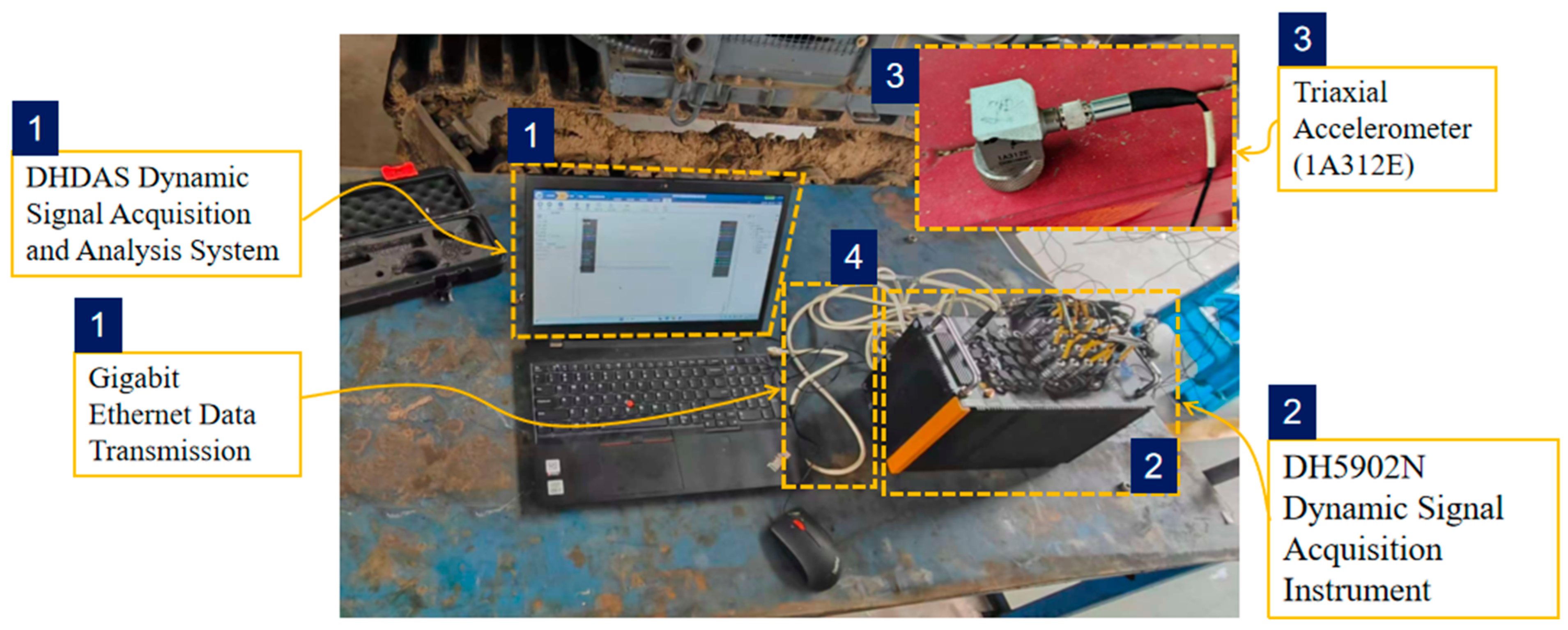
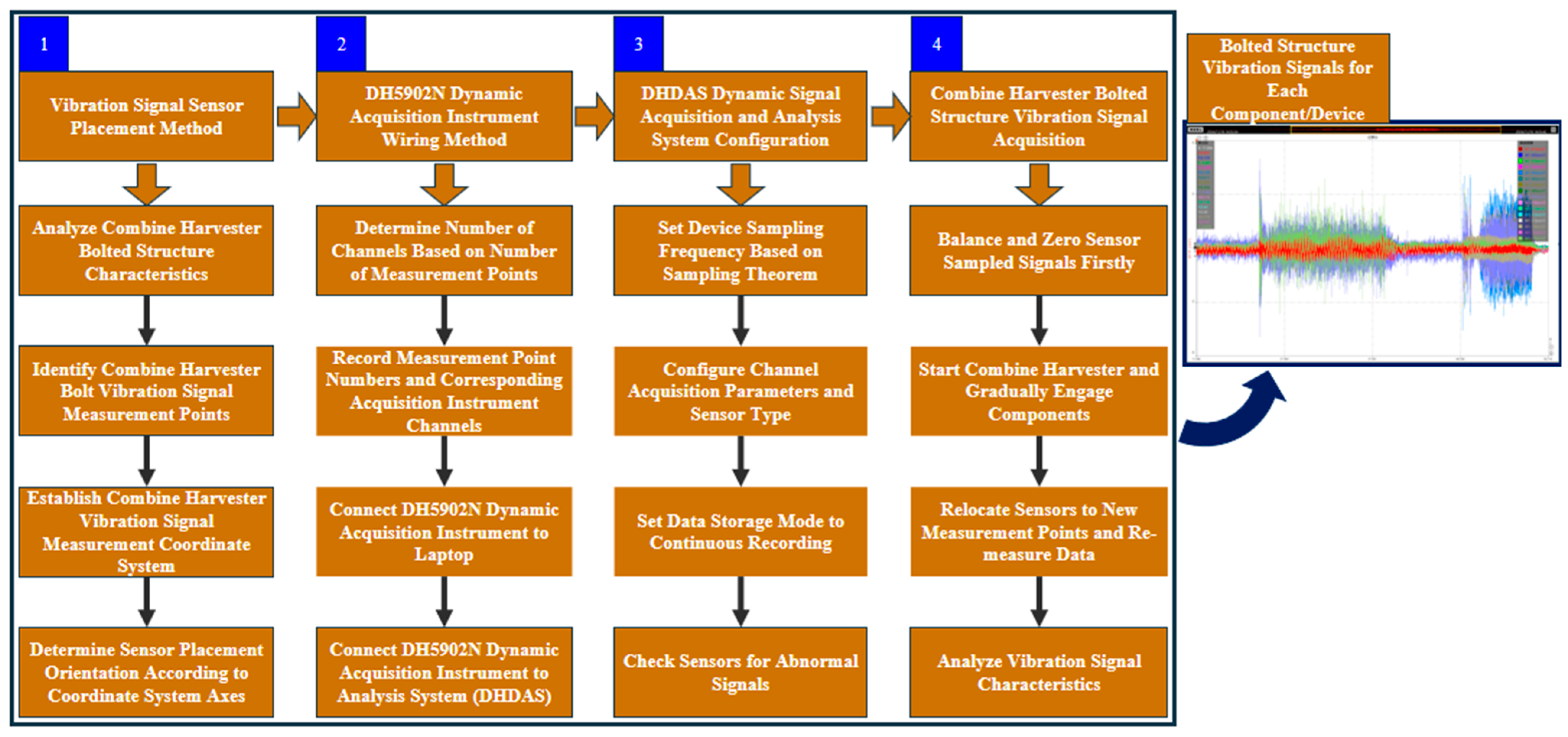
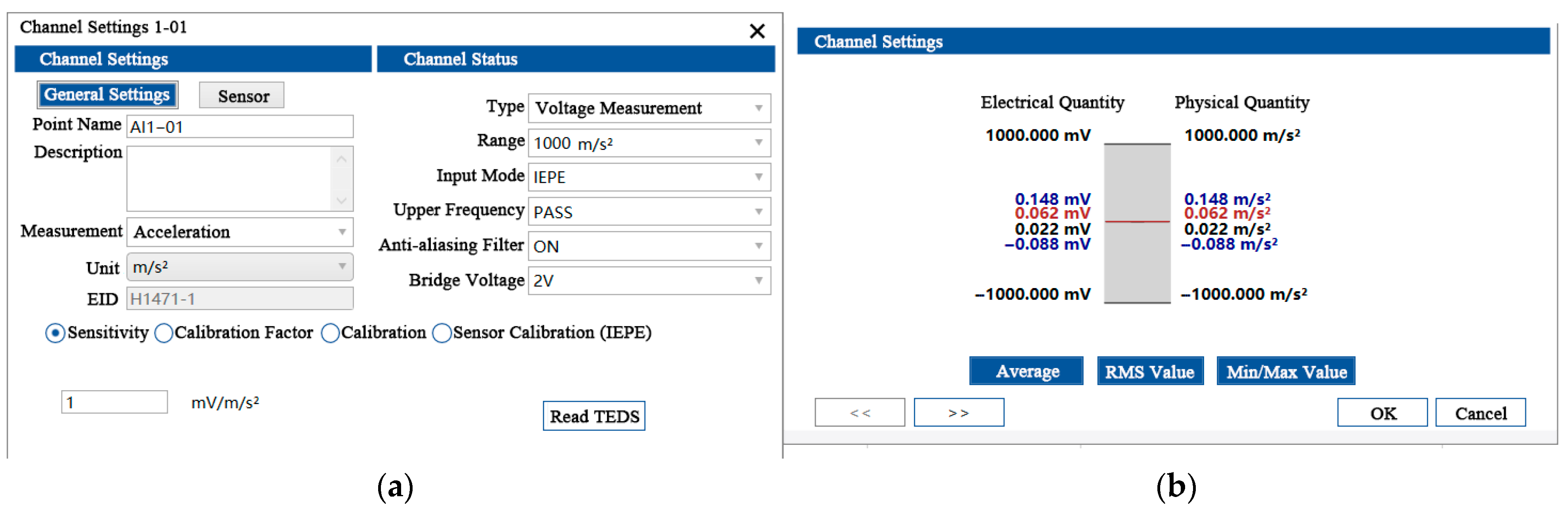
2.1. Signal Acquisition Experiment for the Conveyor Trough and Its Bolted Structure

In this experiment, the primary objective was to acquire the vibration response signals from the bolted structure and connecting components of the combine harvester under time-varying, multi-source excitation conditions. To ensure the scientific validity and accuracy of these signals, the DH5902N Signal Acquisition Instrument and the DHDAS Dynamic Signal Acquisition System, developed by Jiangsu Donghua Vibration Test Technology Co., Ltd. (Jingjiang City, China), were selected. The DH5902N is a rugged data acquisition and analysis system specifically engineered for data collection within challenging environments, such as those found in vehicle-borne, airborne, and shipborne applications. Incorporating an industrial-grade control computer and a solid-state drive (SSD), it is capable of performing testing and extended monitoring tasks under extreme conditions, including intense vibration, wide temperature ranges, and high humidity. Key performance specifications are detailed in

Table 1. DH5902N dynamic signal acquisition instrument.

Order	Parameter	Details
1	Number of Channels	4~32 channels per unit (selectable), expandable to >1000 channels via Ethernet
2	Supported Acquisition Cards	Strain/Voltage/IEPE acquisition cards, Tachometer/Counter cards, Signal source cards, CAN module cards
3	Supported Conditioners	Charge conditioners, Current conditioners, Temperature conditioners
4	A/D Converter per Channel	Independent 24-bit
5	Continuous Sampling Rate	256 kSPS per channel, with range switching (supports massive storage)
6	Communication Interface	Gigabit Ethernet and Wireless Wi-Fi
7	Operating Modes	Online (connected) and Offline (standalone) modes, with seamless switching
8	Power Supply	Battery and/or AC adapter powered; >4 h operation on full charge (for 32 channels)
9	Shock Resistance	100 g/(4 ± 1)ms

.

An overview of the DH5902N Dynamic Acquisition Instrument and the DHDAS Dynamic Signal Acquisition and Analysis System interface is presented in Figure 1. Sensors commonly employed for acquiring dynamic signals in vibration response testing include displacement sensors, velocity sensors, and acceleration sensors. The choice of sensor type influences the measurement based on their respective dynamic performance characteristics, such as frequency response bandwidth and sensitivity. Judging from the overall parameters and specifications of the combine harvester, the frequency response of its bolted structure is expected to be concentrated primarily in the low-frequency band; even harmonics of the rotational frequencies are anticipated to fall within the low-to-mid frequency range. Conversely, noise signals generated due to bolt failure during operation are likely to constitute high-frequency components. Therefore, to ensure the completeness and validity of the experimental signal acquisition across the necessary frequency spectrum, a triaxial piezoelectric accelerometer (Model 1A312E, Jiangsu Donghua Vibration Test Technology Co., Ltd., Jingjiang City, China) was selected.

To investigate the directional vibration responses of the bolted structure at various locations, sensors were required to simultaneously measure acceleration in three orthogonal axes (X, Y, Z). This simultaneous multi-axis measurement guarantees effective subsequent signal analysis. Key parameters for the triaxial accelerometer used are listed in

Table 2. Main specifications and parameters of 1A312E acceleration sensor.

Order	Parameter	Unit	Specification	Order	Parameter	Unit	Specification
1	Frequency Range	Hz	0.5~10,000	4	Weight	g	15
2	Measurement Range	m/s2	5000	6	Operating Temperature	°C	−40~+120
3	Dimensions	mm	16.5 × 16.5 × 16.5	6	Resolution	m/s2	0.01

.

Based on the previously selected test equipment and functional components, a vibration response experiment was formulated for the combine harvester’s bolted structure under time-varying, non-linear, multi-source excitation. The objectives were to investigate the structure’s response characteristics and pinpoint the connections most critically affected by internal vibration, impact, and wear. The experimental procedure is presented in Figure 2.

The research object is the 4LZ-8.0EZ (Q) combine harvester (Jiangsu World Group, Danyang City, China). Firstly, the distribution of internal bolted structure measurement points was determined based on a simplified motion analysis of the conveyor trough and a review of existing research. Focusing primarily on the bolted connections of the main working components as the principal objects of study, six measurement points were established for the acquisition and analysis of bolted structure vibration response signals. To capture the principal vibration directions at each measurement point location, accelerometers were employed for simultaneous signal acquisition in three orthogonal directions. The specific locations and orientations of these measurement points are illustrated in Figure 3. In this experiment, the analysis coordinate system for the vibration response signals was defined as follows: the X-axis was aligned with the primary structural or operational direction relevant to the vibration analysis; the Y-axis was defined as the vertically upward direction relative to the ground plane; and the Z-axis was defined as the direction normal (perpendicular) to the side face of the harvester.

Sensors were mounted onto the combine harvester at the specific measurement point coordinates using magnetic bases. With the exception of measurement points 1, 3, and 4, all other points were located in the vicinity of bolted connection structures. To prevent potential data anomalies caused by sensor cable movement during operation, the wiring was secured using adhesive tape. The accelerometers were connected to the dynamic acquisition system via dedicated instrument cables. Subsequently, the acquisition parameters for the DHDAS dynamic acquisition system were configured as depicted in Figure 4. Given that the exact magnitude of the bolted structure’s response acceleration during harvester operation was unknown a priori, the measurement input range was set to the instrument’s maximum capacity. According to the Nyquist-Shannon sampling theorem, the sampling frequency must be at least twice the highest frequency component anticipated in the signal, as expressed in Equation (1):

$$f_s\ge 2\times f_{\mathit{max}}$$

(1)

To ensure that the original signal components could be reconstructed without loss, the system sampling frequency was set to 2 kHz, thereby satisfying the Nyquist sampling theorem which dictates that the sampling rate must be at least twice the highest frequency present in the signal. System parameters were configured in accordance with the previously specified accelerometer sensitivities. This experiment employed two sensors for simultaneous six-channel signal acquisition. Consequently, acquisition parameters were configured for the necessary six channels within the available channels of the acquisition instrument. Data for the six measurement points were acquired over four distinct measurement runs. The resulting data files were saved using the naming convention “MeasuringDevice-MeasurementSequence”, facilitating clear differentiation between experimental runs and associated measurement point information.

The data acquisition system was configured according to the parameter specifications detailed in Figure 5. The combine harvester was operated continuously until a steady-state condition was reached for all relevant working components. Sampling was performed during this stable operational phase to capture the response signals, specifically obtaining the acceleration response signals at each measurement point along the transverse, vertical, and direction-of-travel axes. Basic processing within the DHDAS system involved applying the Short-Time Fourier Transform (STFT) to the acquired signals. A preliminary plausibility check was performed based on the frequency content and amplitude levels of the signals. Data segments generally conforming to the predefined parameter ranges were subsequently saved for further analysis.

The objective was to determine the principal vibration directions at the bolted connections and fastener locations associated with the conveyor trough, thereby identifying the connections experiencing the most intense vibration. Specific sensor mounting positions and orientation details for each measurement point configuration are documented in

Table 3. The alignment of conveyor trough measurement point orientations with the analysis coordinate system.

Point	Location	Direction Measured	Point	Location	Direction Measured
1	Upper Point at Trough-Header Connection Area	Travel Direction	4	Upper Rear Point at Trough-Header Connection Area	Travel Direction
		Transverse			Transverse
		Vertical			Vertical
2	Side Point at Trough-Header Connection Area	Vertical	5	Upper Point at Rear Trough Connection Area	Transverse
		Transverse			Vertical
		Travel Direction			Travel Direction
3	Upper Front Point at Trough-Header Connection Area	Travel Direction	6	Upper Side Point at Rear Trough Connection Area	Vertical
		Transverse			Travel Direction
		Vertical			Transverse

. Ensuring correct alignment between the sensor’s local X, Y, Z axes and the analysis coordinate system defined in Figure 3 is critical due to the magnetic base mounting. Consequently, meticulous differentiation of the acquired vibration signals according to their corresponding analysis axes is required during the subsequent analysis phase to prevent misinterpretation.

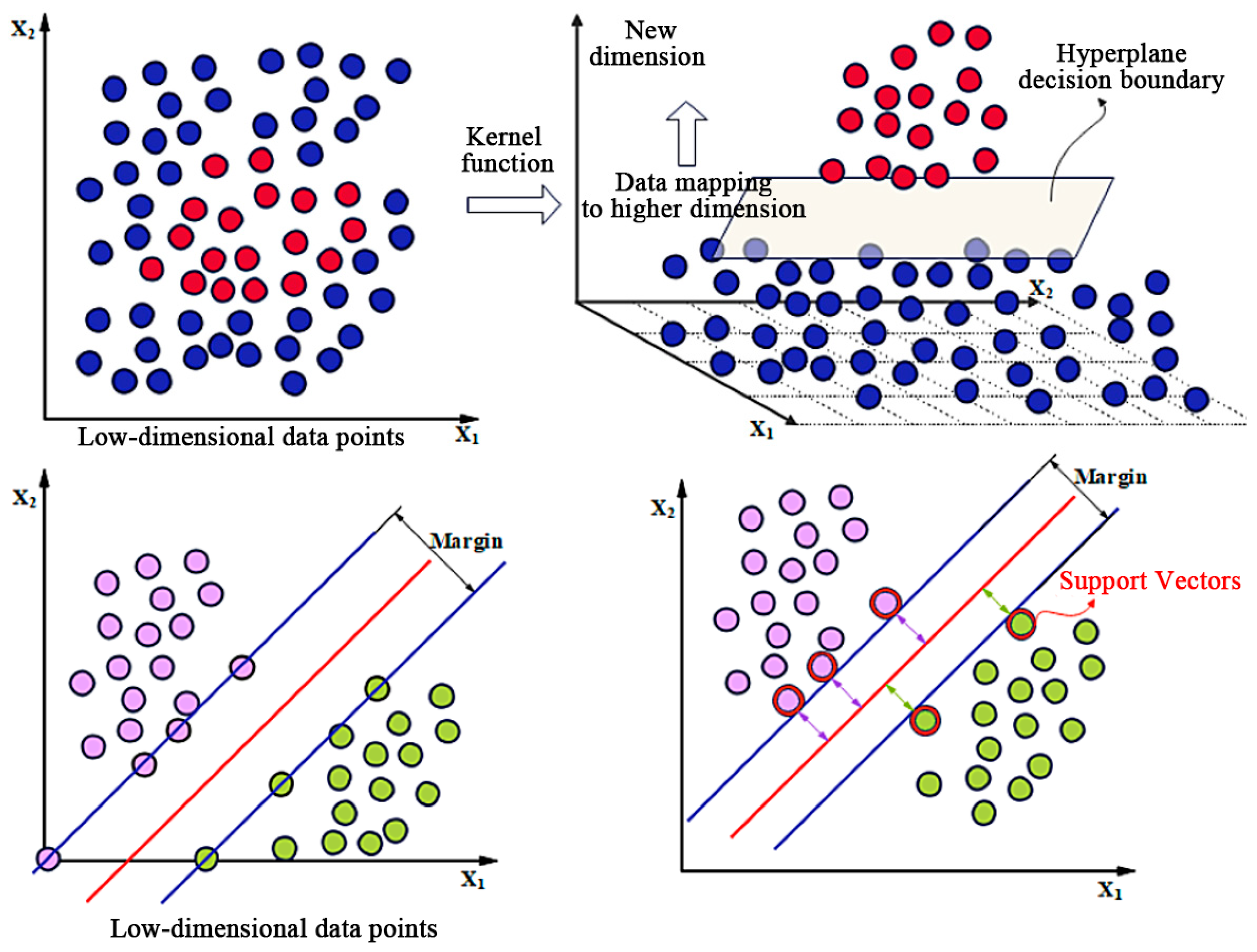
2.2. Support Vector Machine Based Classification and Identification Method

Support Vector Machines (SVM) provide a binary classification framework aimed at constructing an optimal separating hyperplane that maximizes the margin between data classes. Linear SVMs address linearly separable datasets through hard-margin maximization, or nearly separable datasets via soft-margin approaches. For inherently non-linear data, SVM employs the kernel trick, often combined with soft-margin optimization, to establish non-linear decision boundaries. The underlying principles are depicted in Figure 6.

The governing equations and constraints for the linearly separable hard-margin SVM are as follows:

$$\underset{\omega ,b}{Min}{\displaystyle \frac{1}{2}}{‖\omega ‖}^2$$

(2)

$$y_i\left({\omega }^T{X}_i+b\right)\ge 1, \forall i$$

(3)

In the formula: $\omega$—the weight vector of the hyperplane; $b$—the hyperplane bias; $X_i$—the feature vector for the $i$-th sample; $y_i$—the class label of the $i$-th sample. The formulation and associated constraints for the approximately linearly separable soft-margin SVM are as follows:

$$\underset{\omega , b}{M\mathrm{in}}{\displaystyle \frac{1}{2}}{‖\omega ‖}^2+C{\displaystyle \sum _{i=1}^{2n}{\xi }_i}$$

(4)

$$y_i\left({\omega }^T{X}_i+b\right)\ge 1-{\xi }_i, {\xi }_i\ge 0, \forall i$$

(5)

where $C$—the regularization parameter (controlling the penalty associated with misclassifications); ${\xi }_i$—the slack variable (permitting instances of misclassification). The procedure for non-linear SVM (employing the kernel method) is outlined as follows:

$$K\left(X_i,X_j\right)=\phi {\left(X_i\right)}^T\phi \left(X_j\right)$$

(6)

where $K\left(X_i,X_j\right)$—the kernel function; $\phi \left(X\right)$—the mapping to a high-dimensional space. Commonly used kernel functions include the RBF (Radial Basis Function) kernel, the Linear kernel, the Polynomial kernel, and the Sigmoid kernel. Their respective computational formulas are as follows:

$$K\left(X_i,X_j\right)=\mathit{exp}\left(-\gamma {‖X_i-X_j‖}^2\right)$$

(7)

$$K\left(X_i,X_j\right)=X_i^T{X}_j$$

(8)

$$K\left(X_i,X_j\right)={\left(X_i^T{X}_j+c\right)}^d$$

(9)

$$K\left(X_i,X_j\right)=\mathit{tanh}\left(\gamma X_i^T{X}_j+c\right)$$

(10)

where $d$—the degree of the polynomial; $c$—the constant term; $\gamma$—the kernel coefficient. Given that the vibration data from different measurement points might be linearly separable, yet could also exhibit linear inseparability (despite relatively minor amplitude deviations across intervals), the use of multiple kernel functions was deemed appropriate. The prediction method for the resulting trained model is as follows:

$$f\left(x\right)=sign\left({\displaystyle \sum _{i=1}^{2n}{\alpha }_i{y}_{i}K\left(X_i,X_j\right)+b}\right)$$

(11)

where $f\left(x\right)$—the prediction function; ${\alpha }_i$—the Lagrange multipliers. For multi-class classification problems, the “one-vs.-one” strategy is employed. The process entails the following steps: (1) For $k$ distinct classes, all possible pairwise combinations are considered, leading to the construction of $C(k,2)={\displaystyle \frac{k\left(k-1\right)}{2}}$ individual binary SVM classifiers. (2) Each of these binary sub-models is trained independently, using only data from the two specific classes it is designed to distinguish between. (3) During the prediction phase for a new instance, each of the k·(k − 1)/2 classifiers casts a vote for one of the two classes it handles. The final predicted class label is assigned to the class that accumulates the maximum number of votes.

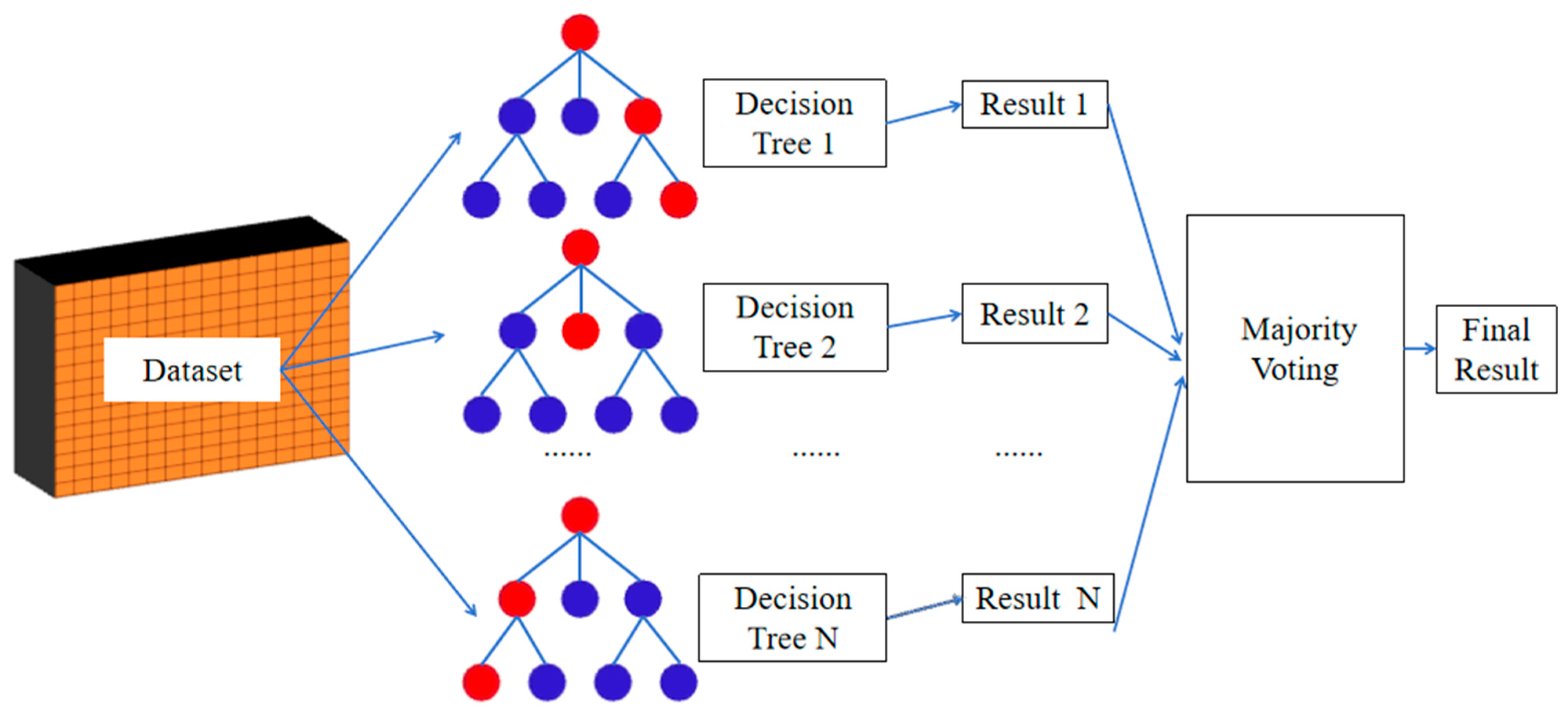
2.3. Random Forest Classification and Identification Method

The Random Forest is an ensemble learning method constructed from multiple decision trees in Figure 7. Each tree within the forest is trained independently. Final predictions are obtained by aggregating the outputs of individual trees, typically through majority voting for classification tasks or averaging for regression tasks, as illustrated in the process flow. The training involves generating k datasets from the original training dataset X using bootstrapping (sampling with replacement). Each of these k datasets is then used to train one decision tree. To determine the optimal split at each node within a tree, criteria such as information gain or the Gini index are commonly employed. Consider a node S containing the sample set {$x_1$, $x_2$, …, $x_i$}, where each sample is associated with a label:

$$Gini=1-{\displaystyle \sum _{k=1}^K{P}_k^2}$$

(12)

where $P_k$—the proportion of samples belonging to class $k$ at the node. The tree construction algorithm selects the feature for splitting that minimizes the Gini index. Each individual tree in the forest predicts a class label for a given input. The final prediction of the Random Forest is determined by aggregating the voting results from all constituent trees:

$$\hat{y}={\displaystyle \frac{1}{T}}{\displaystyle \sum _{t=1}^T{h}_t\left(x\right)}$$

(13)

where $T$—the number of trees; $h_t\left(x\right)$—the prediction of the $t$-th tree.

2.4. Gradient Boosting Tree Classification Method

The Gradient Boosting works by iteratively training each new weak classifier to correct the errors of the classifier from the previous iteration. Assuming the current model is $f_{t-1}\left(x\right)$, firstly, calculate the residuals:

$$r_t=y-f_{t-1}\left(x\right)$$

(14)

where $y$—the true label; $f_{t-1}\left(x\right)$—the predicted value of the current model. Then, based on the residual $r_t$, a new regression tree $h_t\left(x\right)$ is trained, such that the new model reduces the prediction error as much as possible. Its model update method is as follows:

$$f_t\left(x\right)=f_{t-1}\left(x\right)+\eta h_t\left(x\right)$$

(15)

where $\eta$ is the learning rate, used to control the step size of the model update.

2.5. XGBoost, LightGBM, and CatBoost Classification Methods

The goal of XGBoost is to train the model by minimizing an objective function, which consists of a loss function and a regularization term:

$$ℒ\left(\theta \right)={\displaystyle \sum _{i=1}^{N}Loss\left(y_i,{\hat{y}}_i\right)}+{\displaystyle \sum _{k=1}^T\mathrm{\Omega }\left(f_k\right)}$$

(16)

$$\mathrm{\Omega }\left(f_k\right)=\gamma T+{\displaystyle \frac{1}{2}}\lambda {\displaystyle \sum _{j=1}^T{\omega }_j^2}$$

(17)

where $\mathrm{\Omega }\left(f_k\right)$—the regularization term for the tree; $\gamma$ and $\lambda$ —the regularization hyperparameters. Each tree $f_k$ is trained, iteratively updating the model. LightGBM efficiently builds trees by using histogram-based algorithms. Similarly to XGBoost, LightGBM trains by minimizing an objective function. CatBoost places special emphasis on handling categorical features, employing unique encoding strategies (such as target-based encoding) to process categorical data, thereby reducing the need for preprocessing.

2.6. Bayesian Hyperparameter Optimization Method

To enhance the algorithm’s classification performance, the Bayesian optimization method is employed. This utilizes Gaussian Process Regression for modeling to iteratively optimize the hyperparameter search. Stratified K-Fold cross-validation ensures a more robust evaluation of different hyperparameter combinations. The process is illustrated below using the SVM process as an example in Figure 8:

Bayesian optimization uses Gaussian Process Regression (GPR) to estimate the performance of different hyperparameter combinations and selects the next hyperparameter combination to try based on the uncertainty of the estimation. To improve optimization efficiency and classification accuracy, Grid Search is first used to roughly determine the hyperparameter range, and then Bayesian optimization is used to perform a refined search within this range. First, select a wider parameter range:

$$C\in \left\{{10}^{-6},{10}^{-3},{10}^{-1},1,10,{10}^3,{10}^6\right\}, \gamma \in \left\{{10}^{-6},{10}^{-3},{10}^{-1},1\right\}$$

(18)

Firstly, set the hyperparameter range for SVM, the following is an example:

$$C\in \left[{10}^{-6},{10}^6\right], \gamma \in \left[{10}^{-6},10\right], d\in \left[2,3,4,5\right], c\in \left[-1,1\right]$$

(19)

Kernel function selection:

$$K\left(X_i,X_j\right)\in \left[\mathit{Rbf},\mathit{Liner},\mathit{Poly},\mathit{Sigmoid}\right],$$

(20)

And the objective function is:

$$\underset{\theta }{\mathit{max}}\in E\left[\mathit{Accuracy}\left(\theta \right)\right]$$

(21)

where $\theta$—the hyperparameter combination, $\theta =\left(C,\gamma ,d,c,K\right)$; $E\left[\mathit{Accuracy}\left(\theta \right)\right]$—the expected accuracy of SVM cross-validation given hyperparameter $\theta$. Wherein, Bayesian optimization performs modeling using Gaussian Process Regression (GPR):

$$P\left(\left.A\right|\theta \right)~𝒩\left(\mu \left(\theta \right),{\sigma }^2\left(\theta \right)\right)$$

(22)

where $A$—the cross-validation classification accuracy; $\mu \left(\theta \right)$—the mean estimate of the accuracy at hyperparameter $\theta$; ${\sigma }^2\left(\theta \right)$—the variance estimate, representing the uncertainty. Then, the next hyperparameter is selected:

$${\theta }_{\mathit{next}}=\mathit{argmax}\in E\left[\mathit{Accuracy}\left(\theta \right)\right]+\kappa \sigma \left(\theta \right)$$

(23)

where $\kappa$—the exploration weight. Due to potential class imbalance in the data, we adopt Stratified K-Fold cross-validation, dividing the data into k folds. Each time, k−1 folds are selected as the training set, and the remaining 1 fold is used as the validation set. This process is repeated k times to reduce the impact of data partitioning on model performance and the process is:

$$D_{\mathit{train}}=D-D_j,D_{\mathit{val}}=D_j$$

(24)

Train SVM on $D_{\mathit{train}}$, evaluate the model performance on $D_{\mathit{val}}$. The average validation accuracy across the $\kappa$ folds of cross-validation is calculated as the score for the current hyperparameter combination. Based on the SVM optimization process described above, corresponding parameter optimization is performed for Random Forest, Gradient Boosting, XGBoost, LightGBM, and CatBoost. The optimized parameters for each method are shown in

Table 4. Bayesian Optimization Parameter Table for Each Method.

Method	Parameters
Random Forest	Number of decision trees, Maximum depth of decision trees, Minimum samples required to split an internal node, Minimum samples required per leaf node.
Gradient Boosting	Number of decision trees/boosting stages, Learning rate, Maximum depth of each decision tree, Minimum samples for internal node split, Minimum samples per leaf node.
XGBoost	Number of boosting trees, Learning rate, Maximum depth of trees, Proportion of samples used per tree (subsample ratio), Proportion of features used per tree (feature subsample ratio).
LightGBM	Number of trees, Learning rate, Maximum depth of trees, Number of leaves per tree, Minimum number of samples per leaf node.
CatBoost	Number of trees, Learning rate, Depth of trees, L2 regularization coefficient.

.

2.7. Design of the Conveyor Chute Vibration Signal Acquisition System

In the preliminary design of the vibration acquisition system, considering the requirements of the sensors and other modules and for design convenience, 220 V AC is initially used as the power source. The designed circuit converts the 220 V AC into the 5 V and 3.3 V DC power supplies required for the circuitry via a bridge rectifier, a step-down transformer (U1), and linear voltage regulators (U2, U4). The 12 V power supply also be generated to power circuits enabling functions such as overvoltage protection, voltage conversion, signal amplification, and filtering, as shown in Figure 9.

The vibration sensor used in this paper is the analog temperature and vibration sensor model SN-3001-WZ1 (produced by JiNan Puruisen Co., Ltd., Jinan, China). This sensor has a maximum power consumption of 1.2 W, an IP67 protection rating, and is suitable for harsh environments. It supports single-axis vertical vibration measurement, with an operating temperature range of −40 °C to +60 °C and a humidity range of 0~80% RH. The vibration velocity measurement range is 0–50 mm/s, and the detection period is real-time. Other operating parameters are shown in

Table 5. Operating parameters of analog measuring-type SN-3001-WZ1 temperature and vibration sensor.

Parameter	Value or Description	Parameter	Value or Description
Power Supply	DC 10–30 V	Protection Rating	IP67
Max Power Consumption	Current, Voltage output: 1.2 W	Frequency Range	10–1600 Hz or 10–5000 Hz
Vibration Measurement Direction	Single-axis, perpendicular to the measurement surface	Sensor Circuit Operating Temperature	−40 °C~+60 °C, 0%RH~80%RH
Vibration Velocity Measurement Range	0–50 mm/s	Surface Temperature Measurement Range	−40 °C~+80 °C
Vibration Velocity Measurement Accuracy	±1.5% FS (@1 kHz, 10 mm/s)	Output Signal	Current Output: 4–20 mA Voltage Output: 0–5 V/0–10 V
Load Capacity	Current Output: ≤600 Ω Voltage Output: Output Resistance ≤ 250 Ω	Detection Period	Real-time

.

Also, for multi-point vibration signal acquisition on the bolted structure, multi-channel vibration signal acquisition circuits need to be configured. The AD7606, introduced by ADI (Analog Devices, Wilmington, MA, USA), is a high-performance 16-bit, 8-channel simultaneous sampling analog-to-digital converter (ADC) suitable for multi-channel data acquisition systems. It supports sampling rates up to 200 kSPS per channel, and the input voltage range can be software-configured to ±10 V, ±5 V, or ±2.5 V, meeting various signal acquisition requirements. The AD7606 features a typical signal-to-noise ratio (SNR) of 92 dB and total harmonic distortion (THD) down to −100 dB, ensuring the accuracy of signal sampling. It includes an internal 2.5 V reference voltage source and supports both parallel and serial (SPI/QSPI) interfaces, allowing flexible adaptation to different system designs. Furthermore, the AD7606 employs a low-power design with a typical power consumption of 100 mW and an operating temperature range of −40 °C to +85 °C. Therefore, the high-precision ADS1299 (Texas Instruments, Chengdu, China) is used as the acquisition module for the sensor, as shown in Figure 10.

Considering the need to interface with external 5 V logic level peripherals and components connected to this vibration acquisition system, and given the 3.3 V operating voltage of the main controller, a 3.3 V to 5 V logic level conversion module, as depicted in Figure 11, is required. The module is designed to convert 3.3 V logic level signals to 5 V logic level signals, implementing an inverting conversion. Each individual circuit unit (Q1–Q8) independently performs level conversion for a single signal path. The complete module provides eight channels of 3.3 V to 5 V inverting level conversion paths, intended for connecting 3.3 V logic control circuits to external peripherals or components requiring 5 V logic levels.

The main controller of the signal acquisition system employs the A39C-T400A22D1a wireless communication chip from Zeya Microelectronics (Bengaluru, India). Empirical testing demonstrates a maximum wireless transmission distance of up to 5000 m, with an air data rate of 1.2 to 62.5 kbps, as indicated in Figure 12. High-precision data acquisition is achieved through controlling the ADS1299 ADC module, ensuring the accurate capture of analog vibration signals. The acquired digital vibration data undergoes processing, such as filtering, analysis, or format conversion. The system is also responsible for external communication, and via UART serial and SPI interfaces, the system facilitates data exchange and command reception with external devices (e.g., host computers or data logging equipment). The circuit further incorporates a GPIO expansion interface (P1 Header 11) to connect and control additional peripheral modules, enabling enhanced functional capabilities, such as alarm indication, status display, or connection of additional sensors. To facilitate software development and system debugging, the module further integrates an SWD debugging interface (P11), thereby facilitating circuit program development, firmware flashing, and online debugging functionalities.

The overall system architecture is illustrated in Figure 13. The signal acquisition system hardware equipment comprises a circuit board, which incorporates eight channels of acquisition interfaces. Interface and debugging interfaces are included. In addition to power supply lines, power supply modules, and temperature vibration sensors, a wireless transmitting end is also incorporated. An antenna and a wireless receiving end are included. Within these, the circuitry of the wireless receiving end, in conjunction with a USB serial port debugging assistant, is pluggable into laptop computers, small PCs, and other host computer devices. PC machines and other host computer devices are connectable.

To enable communication with the signal acquisition system, a host computer system design is also necessitated. This host computer system design encompasses the acquisition of data from multiple sensors, as well as real-time display functionalities. The host computer software and the programming of the wireless receiving end are designed based on serial communication principles and utilizing the Python 3.12.5 programming language. As illustrated in Figure 14, the functionalities of the host computer system include signal display settings, real-time signal waveforms, legends, serial port connection information, data logging, file export, and command interaction functionalities.

In consideration of the SN-3001-WZ1 analog temperature-vibration sensor being categorized into current-type and voltage-type output signals, and in conjunction with the acquisition module principle of the ADS1299, the calculation process for acquired signals is presented below. The calculation formula for converting the raw ADC value of current-type output to voltage is as follows:

$$V_{\mathit{input}}={\displaystyle \frac{D}{2^{15}}}\times V_{\mathit{ref}}$$

(25)

wherein: $D$—the 16-bit signed integer output from the AD7606; $V_{\mathit{ref}}$—the reference voltage of the AD7606; $V_{\mathit{input}}$—the actual voltage value at the input terminal of the ADS1299. The calculation formula for converting voltage to vibration velocity $V_{\mathit{vibration}}$ is as follows:

$$V_{\mathit{vibration}}=12.5\times \left(V_{\mathit{input}}-1\right)$$

(26)

In the calculation of voltage from the raw ADC values of voltage-type output, beyond the calculation of voltage from the raw ADC values after voltage division associated with current-type output, restoration of the original voltage is also necessary. The formula is as follows:

$$V_{\mathit{original}}={\displaystyle \frac{V_{\mathit{scaled}}\times 10}{V_{\mathit{ref}}}}$$

(27)

Subsequently, the vibration velocity signal can be calculated based on the original voltage, with its calculation method as follows:

$$V_{\mathit{vibration}}=V_{\mathit{original}}\times 5$$

(28)

For the precision of data, the calibration of the signal and error correction are also necessary, with its zero-point calibration method being:

$$D_{\mathit{corrected}}=D_{\mathit{raw}}-D_{\mathit{zero}}$$

(29)

wherein: $D_{\mathit{raw}}$—the uncalibrated ADC output value; $D_{\mathit{zero}}$—the ADC output value at zero-point calibration (corresponding to 4 mA or 0 V). $D_{\mathit{corrected}}$—the ADC output value after zero-point calibration. The full-scale calibration formula is:

$$V_{\mathit{vibration}}=\left({\displaystyle \frac{D_{\mathit{corrected}}}{D_{\mathit{full}}-D_{\mathit{zero}}}}\right)\times 50$$

(30)

wherein: $D_{\mathit{full}}$—the ADC output value at full-scale calibration (corresponding to 20 mA or 10 V). The vibration displacement signal from the sensor is sampled and quantized by an analog-to-digital converter (AD7606) at a fixed time interval (sampling period). Consequently, the acquired vibration displacement signal is a discrete signal. For discrete signals, vibration acceleration can be calculated using the finite difference method:

$$a_{\left[n\right]}=\frac{v_{\left[n\right]}-v_{[n-1]}}{\Delta t}$$

(31)

wherein: $v_{\left[n\right]}$—the vibration velocity value at the current sampling point. $v_{[n-1]}$—the vibration velocity value at the preceding sampling point. The sampling interval time is represented by $\Delta t$ ($\Delta t={\displaystyle \frac{1}{f_s}}$, $f_s$ is the sampling rate).

3. Results and Discussion

3.1. Feature Analysis of Vibration Signals in Conveyor Trough Bolt Structure

The time-domain characteristics in the X-direction are as shown in Figure 15. In Interval 1 (idling), the root mean square (RMS) values for all measurement points are relatively low (generally below 0.9). Upon entering Interval 2 (device disengagement from the drum and start-up), signal enhancement is observed across all measurement points, although the magnitude of increase varies significantly. The increase in amplitude for measurement points 1 to 4 is relatively minor, whereas the RMS value for measurement point 6 increases significantly from 0.797 to 2.524, indicating a strong response of this measurement point during the start-up process. The RMS value for measurement point 5 surges from 0.849 in idling to 4.642, demonstrating an exceptionally strong response of this point to the device disengagement/start-up event; this measurement point is located on the outer side of the disengagement drum impact. In Interval 3 (cutterbar start-up), the vibration signals are further enhanced, reaching peak values. The RMS values for measurement points 1 to 4 increase to 1.6–2.0. The RMS value for measurement point 6 further increases to 3.896, while the RMS value for measurement point 5 reaches 6.650, significantly exceeding its own values in other intervals and other directions, and also far surpassing the values of all other measurement points under any condition. It is evident that the X-direction at measurement point 5 is the location with the largest response within the entire system.

The Y-directional time-domain characteristics are presented in Figure 16. During Interval 1 (idling), characteristic values for most measurement points are low, yet measurement points 1 (1.415) and 5 (3.399) exhibit comparatively elevated values, particularly measurement point 5. Upon entry into Interval 2 (device disengagement from drum and start-up), measurement point 3′s Y-directional RMS value demonstrably increases from 1.109 to 2.736, displaying a marked amplitude augmentation and signifying its Y-directional sensitivity to the start-up process. Measurement point 4′s Y-directional RMS value (0.656 to 1.758) also shows a significant increment. Conversely, measurement point 5′s Y-directional RMS value in Interval 2 declines from 3.399 to 2.253, suggesting a degree of vibration suppression attributed to the disengagement drum start-up. Within Interval 3 (cutterbar start-up), measurement point 3′s Y-directional response is most prominent, its RMS value reaching 4.628, substantially exceeding its X and Z-directional values and all other Y-directional values, except for measurement point 5 during idling. This unequivocally establishes measurement point 3 as the primary locus of Y-directional load or vibration concentration and maximal sensitivity during cutterbar operation.

The Z-directional time-domain characteristics are presented as illustrated in Figure 17. In contrast to X and Y directions, Z-directional signal responses exhibit a comparatively tempered overall intensity and incidence of anomalies, failing to indicate localized issues or pronounced stress concentrations akin to those observed in X and Y directions. During Interval 1 (idling), Z-directional RMS values across all measurement points universally reach their nadir, predominantly remaining below 1.0. Upon entry into Interval 2 (device disengagement from drum and start-up), measurement points 2 (RMS 1.455) and 5 (RMS 1.815) display relatively elevated Z-directional values, yet without exhibiting order-of-magnitude transitions, suggesting a more dispersed Z-directional excitation during device start-up, precluding the formation of pronounced stress concentrations. By Interval 3 (cutterbar start-up), Z-directional RMS values for measurement points 2 (RMS 2.128) and 4 (RMS 2.041) are comparatively higher, indicating that these locations sustain greater vertical vibration or load during cutterbar operation.

In overall perspective, measurement point 5 emerges as the system’s paramount anomaly, exhibiting an acutely elevated X-directional response during both device and cutterbar start-up phases (Intervals 2 and 3). Under conditions of high load, particularly during cutterbar initiation, the conveyor trough’s dynamic response manifests saliently at specific locations (P5, P3, P6) and directions (P5-X, P3-Y, P6-X). Consequently, subsequent diagnostics should prioritize measurement point 5 in the X-direction, followed by measurement point 3 in the Y-direction and measurement point 6 in the X-direction as secondary foci.

3.2. Recognition Result Analysis Under Bayesian Hyperparameter Optimization

To analyze interval-specific characteristics of measurement point 5 in the X-direction of the conveyor groove bolt structure, and to enhance efficacy in interval classification recognition, a multiplicity of features were extracted for categorization. This paper, therefore, applies recognition classification across both time and frequency domains, with employed features enumerated in

Table 6. Classification signal characteristics of the conveyor groove bolt structure.

Time-Domain Features		Frequency-Domain Features
Mean	Kurtosis Factor	Center Frequency	Spectral Kurtosis
Root Mean Square	Mean Absolute Value	Bandwidth	Spectral Flatness
Variance	Integrated Absolute Value	Frequency Energy Ratio	Spectral Entropy
Standard Deviation	Zero Crossing Rate	Harmonic Component Energy	Instantaneous Frequency Mean
Peak Value	Root Sum of Squares	Sideband Energy	Frequency Component Count
Peak-to-Peak Value	Absolute Mean Deviation	Spectral Centroid (Value equals Center Frequency)	Dominant Frequency Component Amplitude
Kurtosis	Energy	Spectral RMS Frequency
Skewness	Autocorrelation Coefficient_lag1	Spectral Variance
Waveform Factor	Hilbert Envelope Energy Mean	Spectral Skewness
Mean	Kurtosis Factor (Value equals Kurtosis)	Center Frequency

.

For the purpose of constructing a classification dataset, the signal characteristics of measurement point 5 (X-direction) for each interval of the conveyor trough were segmented into 500 instances each. Time-domain and frequency-domain features were extracted from each segment to compile the dataset. Data labels were subsequently assigned to the datasets for each interval, followed by discriminative classification utilizing SVM, Random Forest, Gradient Boosting Tree, XGBoost, LightGBM, and CatBoost classifiers. Analysis results pertaining to Interval 1 and Interval 2 are presented in

Table 7. The method optimized the full feature recognition rate of all the parameters (Interval 1 and Interval 2).

Method	Recognition Rate	Optimal Parameters	Cross-Validation
SVM	97.67%	Regularization Parameter 10, Kernel Function RBF, Kernel Scale	96.57%
Random Forest	95.67%	Number of Decision Trees 229, Maximum Depth 13, Minimum Samples Required to Split Internal Node 3, Minimum Samples in Leaf Node 6	95.71%
Gradient Boosting Tree	96.67%	Number of Trees 88, Learning Rate 0.15, Maximum Depth of Decision Tree 3, Minimum Samples Required to Split Internal Node 5, Minimum Samples in Leaf Node 2	96.29%
XGBoost	97.00%	Number of Boosting Trees 200, Learning Rate 0.2, Tree Depth 8, Subsample Ratio for Training Each Tree 0.5, Feature Ratio for Training Each Tree 1	97.00%
LightGBM	96.67%	Number of Trees 173, Learning Rate 0.2, Tree Depth 8, Number of Leaf Nodes per Tree 20, Minimum Samples Required in Leaf Node 41	96.43%
CatBoost	96.67%	Number of Trees 67, Learning Rate 0.09, Tree Depth 7, L2 Regularization Coefficient 3.96	96.00%

.

Among the six algorithms compared (SVM, Random Forest, Gradient Boosting Tree, XGBoost, LightGBM, CatBoost), Support Vector Machine (SVM) demonstrates superior efficacy, achieving a recognition rate as high as 97.67% under optimal parameter configuration (Regularization Parameter 10, Radial Basis Function Kernel RBF, Kernel Scale Parameter scale 1). The recognition rate of the Bayesian-optimized SVM method is particularly noteworthy, with results illustrated in Figure 18. Subsequently, XGBoost closely follows with a recognition rate of 97.00%.

Moreover, the peak cross-validation score of 97.00% underscores the model’s robust stability. Algorithms employing gradient boosting trees (Gradient Boosting Trees, LightGBM, CatBoost) also performed commendably well, all achieving a 96.67% recognition rate. Ultimately, based on the final recognition accuracy on the test set, SVM was identified as the optimal model for this specific binary classification problem.

As shown in

Table 8. The method optimized the full feature recognition rate of all the parameters (Interval 2 and Interval 3).

Method	Recognition Rate	Optimal Parameters	Cross-Validation
SVM	97.67%	Regularization parameter 10, Kernel function RBF, Kernel coefficient scale	95.15%
Random Forest	96.00%	Number of decision trees 70, Maximum depth 9, Minimum number of samples required for splitting internal nodes 2, Minimum number of samples required for leaf nodes 3.	93.29%
Gradient Boosting Tree	95.00%	Number of trees 100, Learning rate 0.20, Maximum depth of decision tree 8, Minimum number of samples for splitting internal nodes 5, Minimum number of samples for leaf nodes 10.	95.29%
XGBoost	95.67%	Number of boosting trees 193, Learning rate 0.2, Tree depth 5, Sample ratio used when training each tree 0.92, Feature ratio used when training each tree 0.93.	95.00%
LightGBM	95.33%	Number of trees 78, Learning rate 0.09, Tree depth 8, Number of leaf nodes in the tree 60, Minimum number of samples required in leaf nodes 25.	95.43%
CatBoost	95.33%	Number of trees 142, Learning rate 0.10, Tree depth 6, L2 regularization coefficient 3.13.	95.71%

and Figure 19, the recognition results for Interval 2 and Interval 3 are as follows. The model achieves 98.67% accuracy in identifying Interval 2 samples and 96.67% for Interval 3 samples. Notably, the primary error is the model misclassifying 3.33% of Interval 3 samples as Interval 2. The ‘Recognition Result Scatter Plot’ demonstrates an overall accuracy of 97.6667%. Evidently, the Support Vector Machines are better suited for classifying vibration signals of conveying trough bolted structures.

Furthermore, based on the “one-vs.-one” (OvO) strategy and using three intervals as the dataset for training, the results are presented in Figure 20, the model correctly identified 99.6% of Interval 1 samples, 98.2% of Interval 2 samples, and achieved perfect recognition of Interval 3 samples at 100.0%. The non-diagonal elements reveal minimal misclassification: only 0.4% of Interval 1 samples were misclassified as Interval 2, and 1.8% of Interval 2 samples were misclassified as Interval 1, with all other types of confusion being zero. Overall, the accuracy is clearly very high, and the recognition of Interval 3 is remarkably accurate, with only very slight and manageable confusion between Interval 1 and Interval 2.

3.3. Performance Testing of Signal Acquisition System

To verify the performance of the signal acquisition system, the sensor and acquisition device are installed near the bolted connection structure of the combine harvester. After starting the machine, the performance of the signal acquisition system is tested. The installation and testing setup of the acquisition system is shown in Figure 21.

The test results from the host computer demonstrate that this acquisition system, employing a high-performance AD7606 analog-to-digital converter, achieves a 16-bit resolution, enabling the acquisition of 65,536 distinct digital levels. With the system’s full-scale range configured for vibration signal acquisition up to 50 mm/s, it is theoretically capable of resolving minute vibration variations at a level of approximately 0.00076 mm/s (calculated as 50 mm/s divided by 65,536). Furthermore, the AD7606 facilitates 8-channel synchronous sampling, with each channel exhibiting a maximum sampling rate of 200 kSPS and acquiring 16-bit data. Consequently, the aggregate data throughput for eight channels is calculated as 8 × 200 kSPS × 16 bits/sample = 25.6 Mbps. Despite the A39C-T400A22D1a wireless transmission chipset requiring only approximately 0.8 s for data transmission, even considering overheads such as data packet headers and control information, the Mbps-level SPI rate is demonstrably sufficient to satisfy the real-time transmission requirements for high sampling rate vibration data from eight channels. Therefore, this acquisition system exhibits the capability for efficient acquisition and analysis of high-frequency vibration signals, supporting the acquisition of vibrational phenomena with frequencies reaching 100 kHz and beyond, without incurring data loss attributable to data transmission limitations.

To validate the efficacy of the proposed state recognition method, integrating the designed signal acquisition system and the aforementioned recognition methodology, a module-based recognition program was designed for the host computer. Consequently, the measurement data from intervals 1, 2, and 3 were designated as the model training dataset, with real-time data acquired by the sensors serving as the validation dataset for recognition testing. The experimental procedure is depicted in Figure 22, and comprises the following steps: (1) Import the raw training dataset file (File 1), which encompasses intervals 1~3 as the training intervals, and extract 500 signals from each interval as a training dataset. (2) Import the data file for validation (File 2), containing intervals 4~6 as the evaluation intervals. (3) Train the model and subsequently validate the dataset.

The validation results are presented in Figure 23. It is evident that for Work State 1 (Interval 1), the classification accuracy is 96.9%, with a misclassification rate of 2.9% as Interval 2, and a misclassification rate of 0.1% as Interval 3. For Work State 2 (Interval 2), the classification accuracy is 97.0%, with a misclassification rate of 2.7% as Interval 1, and a misclassification rate of 0.3% as Interval 3. For Work State 3 (Interval 3), the classification accuracy is 99.7%, with a misclassification rate of 0.1% as Interval 1, and a misclassification rate of 0.2% as Interval 2. The misclassification rates for other intervals are all below 5%. It can be concluded that precise identification of the working state of the bolted structure is achievable.

4. Conclusions

(1)

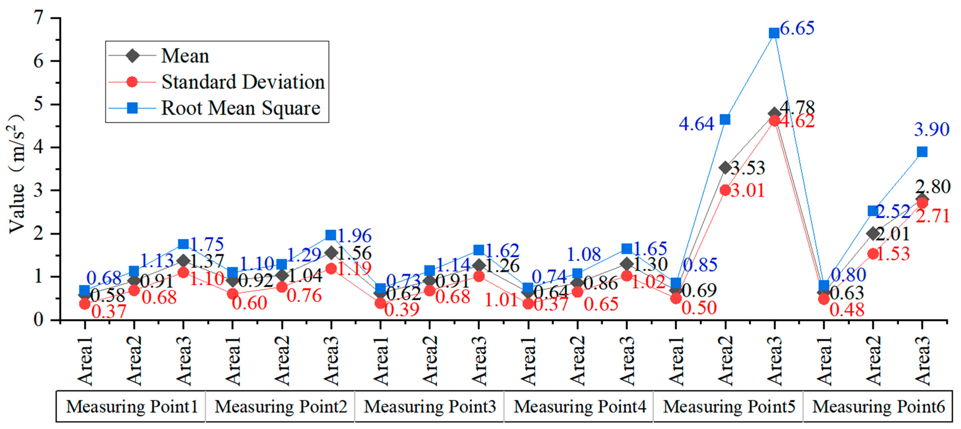
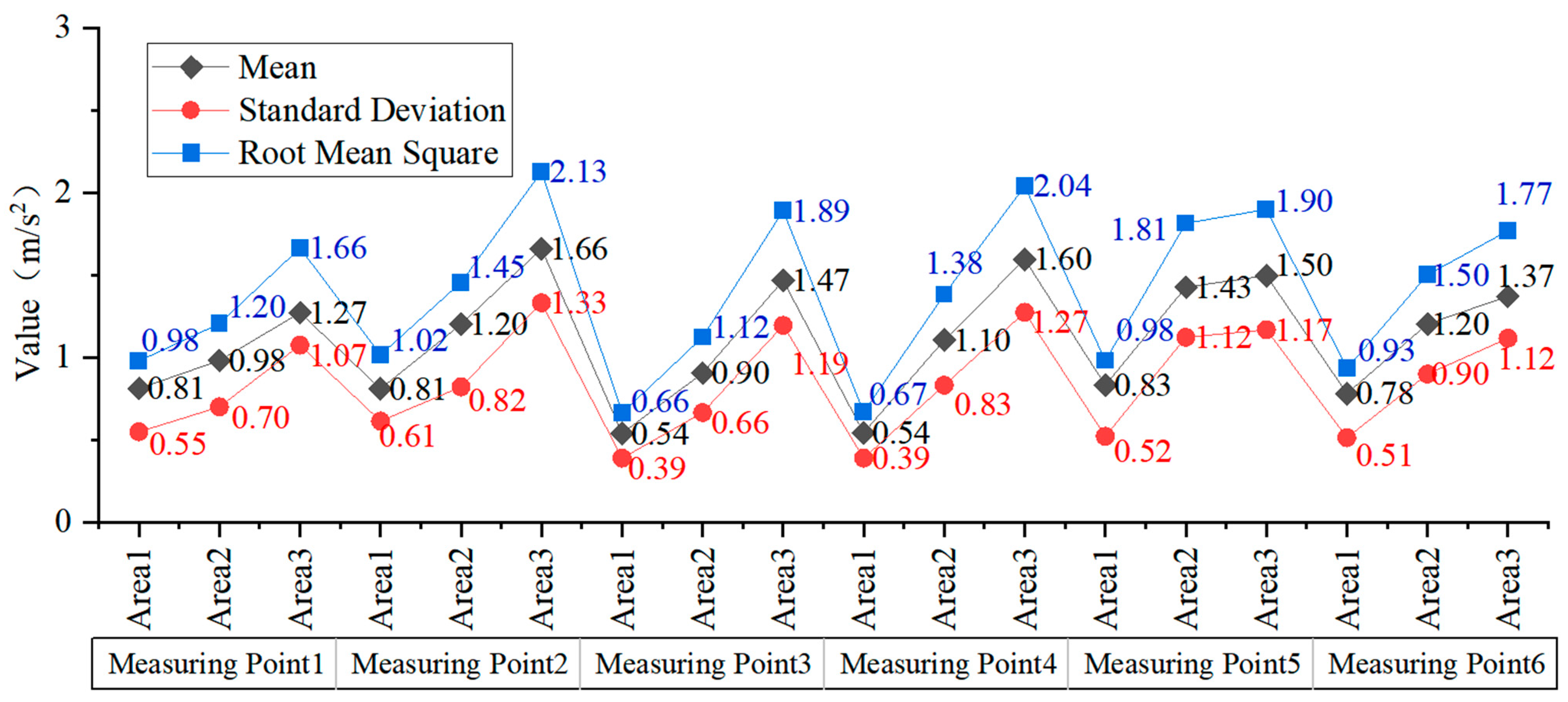
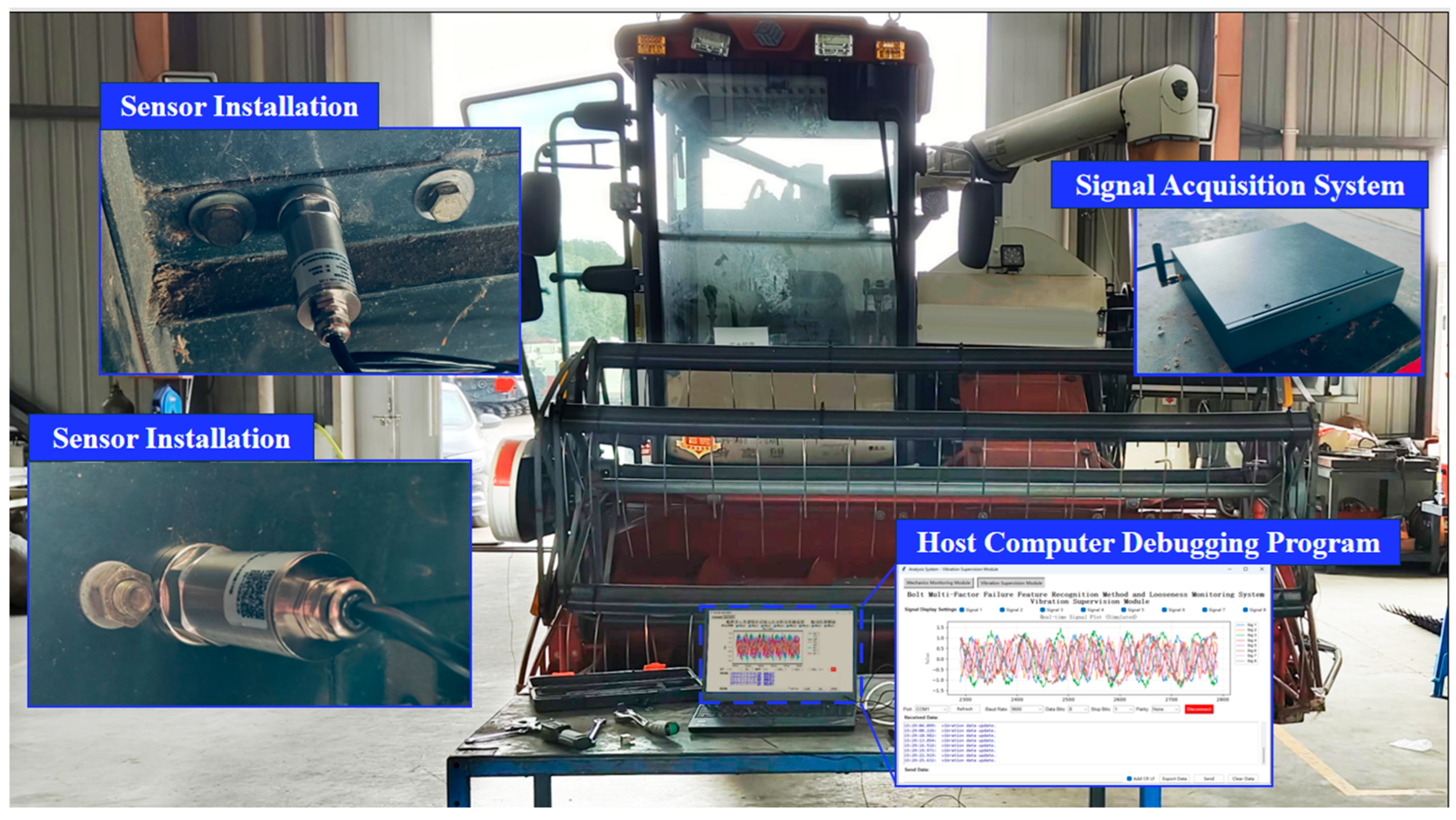
Based on signal acquisition experiments conducted on the conveying trough structure, a time-domain and frequency-domain analysis was performed on the bolted structures of the conveying trough. By comparing the time-domain characteristics across various measurement points, the location exhibiting the most pronounced signal response in the conveying trough and at the bolted connections was identified. It was observed that the bolted connection between the conveying trough and the threshing unit frame (measurement point 5) demonstrated the most significant response. Specifically, the RMS value in the X-direction at measurement point 5 surged from 0.849 during idling to 4.642 in Interval 2 (device start-up), and further escalated to a peak value of 6.650 in Interval 3 (header start-up), indicating a high response and substantial dynamic strain at this location. Subsequently, the Y-direction at measurement point 3 also exhibited a considerable response during Interval 3 (header start-up), with an RMS value reaching 4.628. Concurrently, the RMS value in the X-direction at measurement point 6 also increased significantly to 3.896 in Interval 3, suggesting that the threshing unit actively bears a substantial vibration load. In contrast, the Z-direction response was generally moderate across all measurement points, with peak values only reaching approximately 2.1, thereby establishing a foundational understanding for subsequent state assessment.

(2)

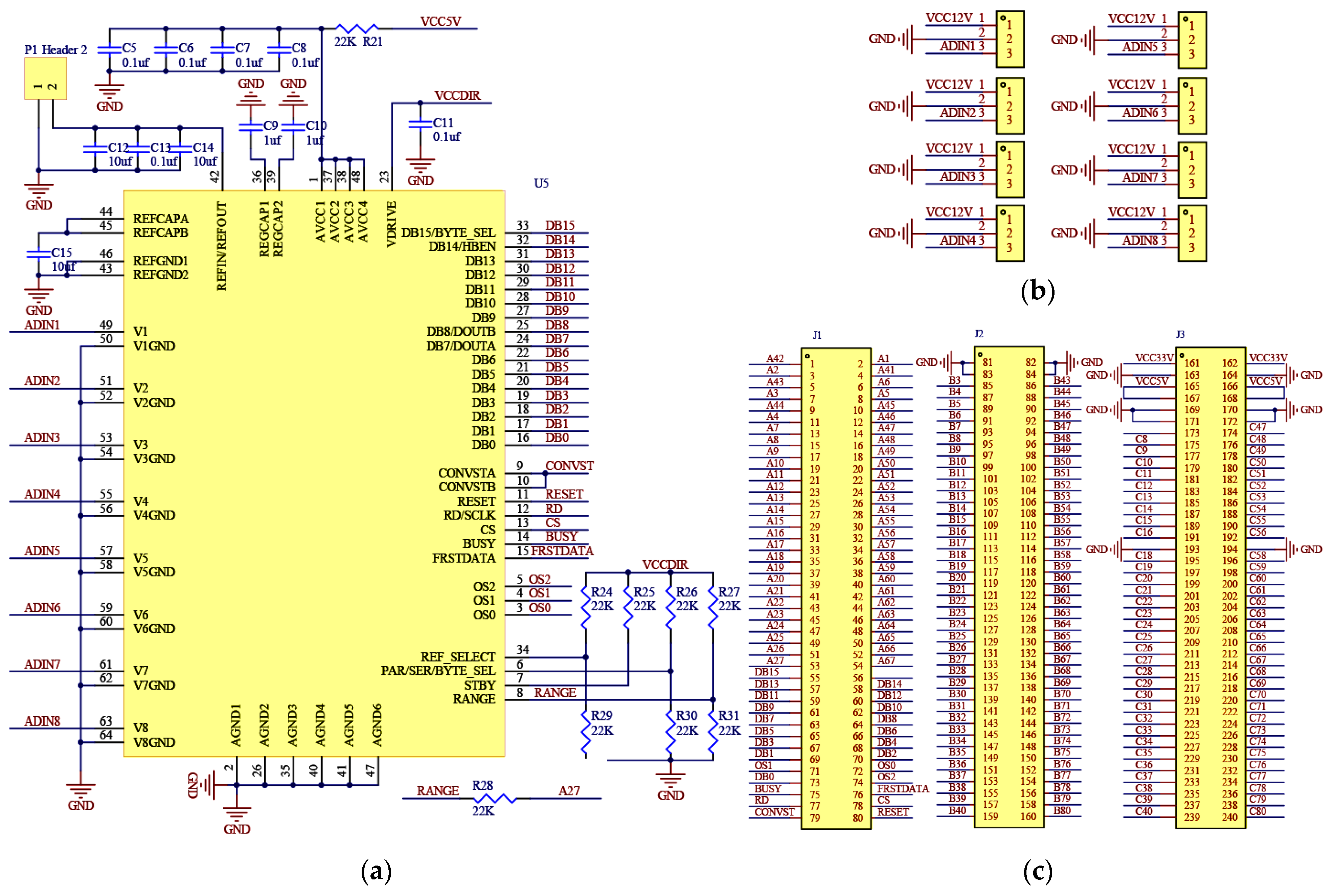
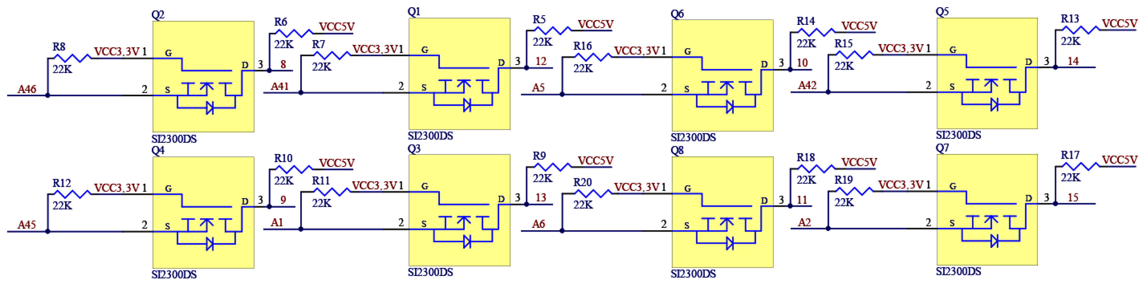
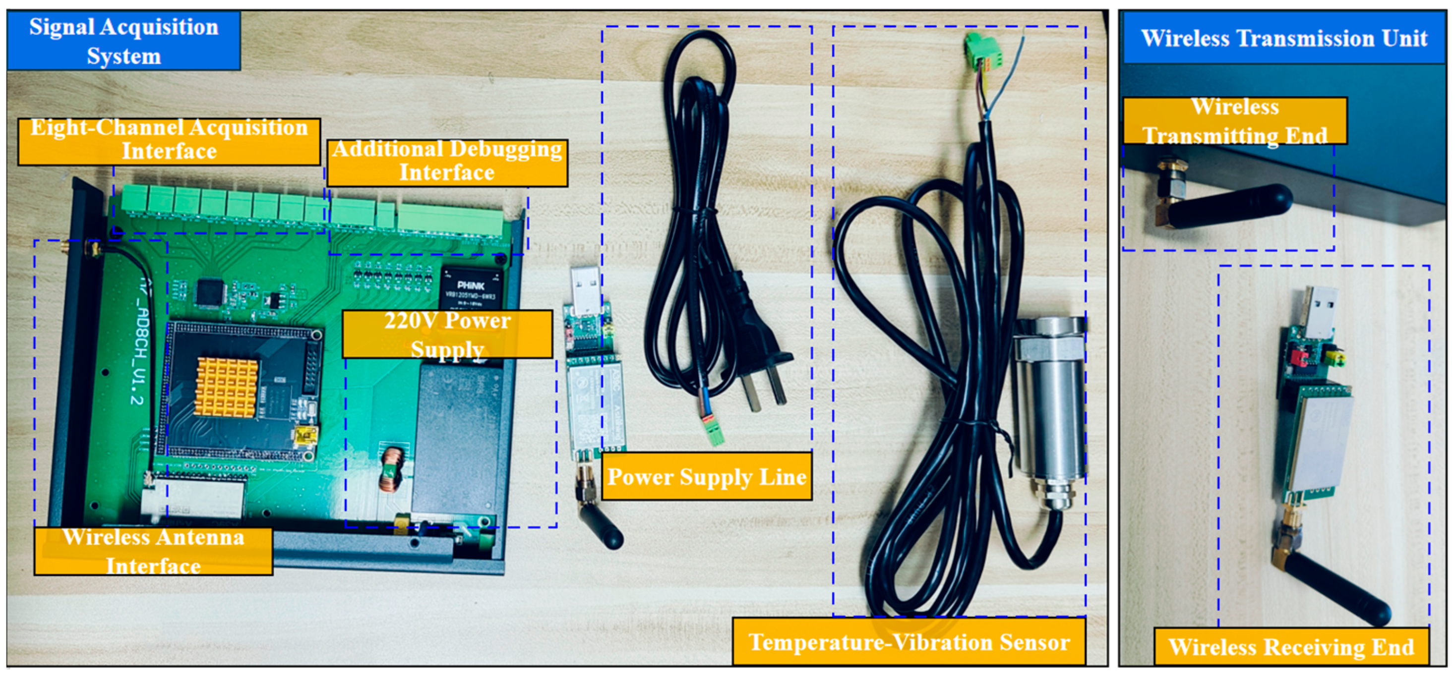
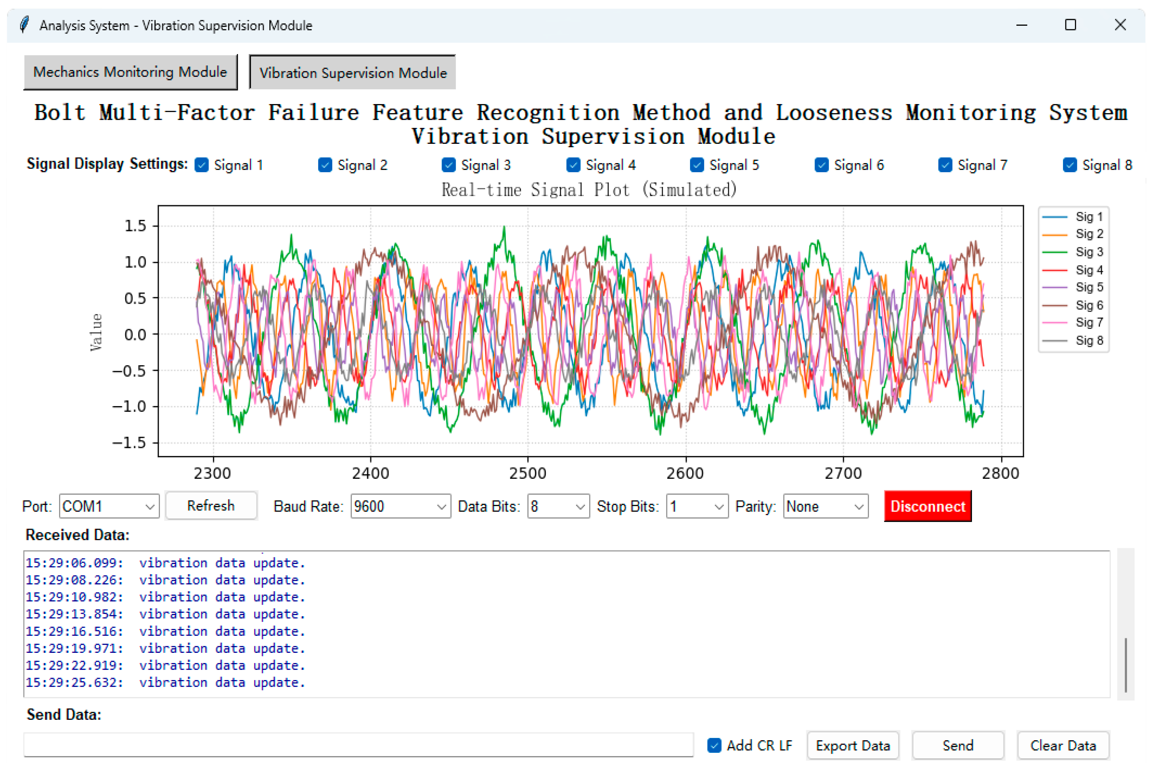
By integrating the high-performance AD7606 analog-to-digital converter and A39C-T400A22D1a wireless transmission technology, a vibration signal acquisition system was designed, capable of achieving a 16-bit resolution, which facilitates the acquisition of 65,536 distinct digital levels. The system, with its full-scale range corresponding to 50 mm/s vibration signal acquisition, is theoretically capable of resolving minute vibration variations on the order of 0.00076 mm/s (calculated as 50 mm/s/65,536). Furthermore, the acquisition system supports 8-channel synchronous sampling, with each channel possessing a maximum sampling rate of 200 kSPS and acquiring 16-bit data. Utilizing the A39C-T400A22D1a wireless transmission chipset, data transmission can be completed in approximately 0.8 s. The system is, therefore, capable of meeting the real-time transmission demands of 8-channel high sampling rate vibration data. Concurrently, the system supports the acquisition of vibration signals with frequencies up to 100 kHz or even higher, ensuring that data loss due to transmission limitations is avoided. Consequently, the designed system is deemed suitable for acquiring information pertaining to the vibration state of the conveying trough bolted structure.

(3)

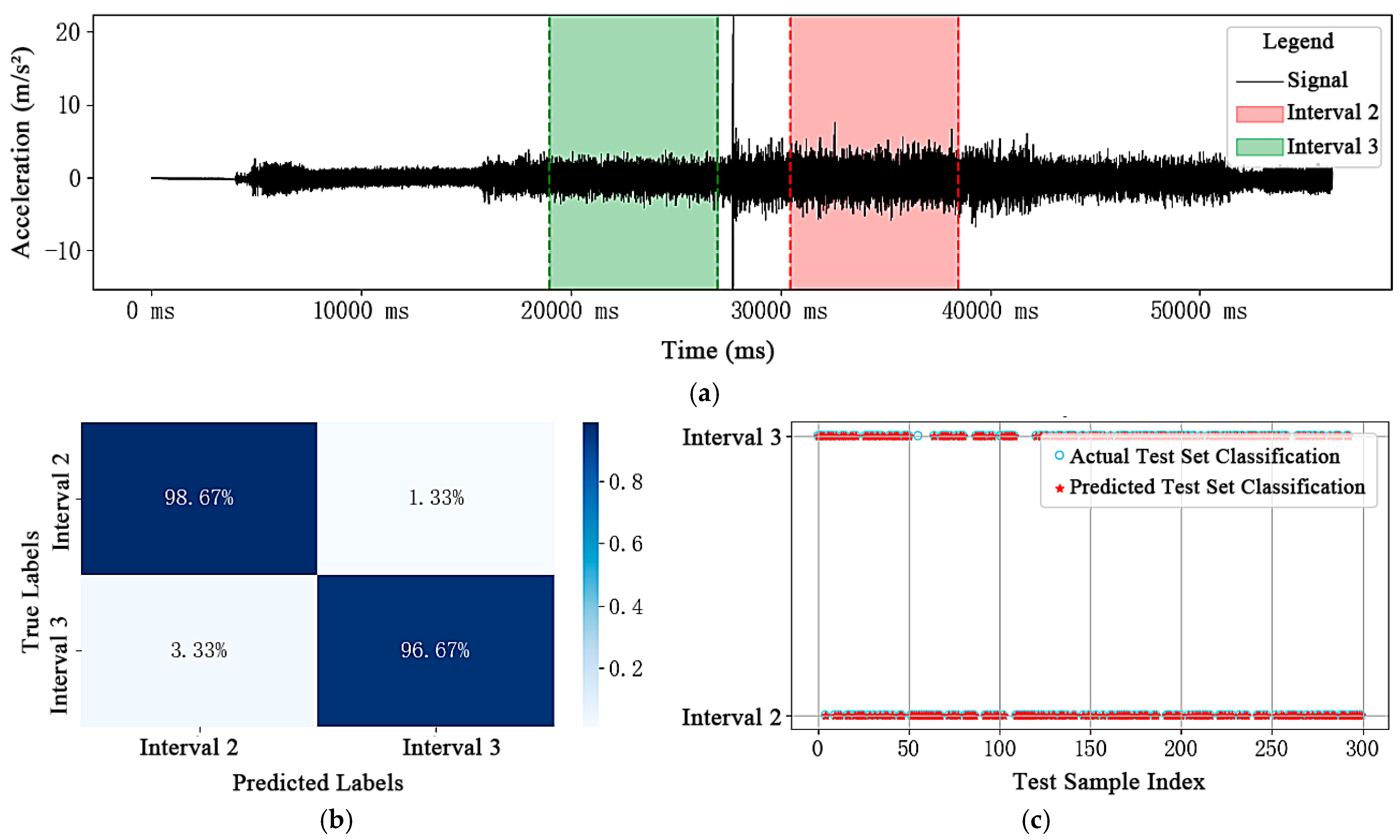
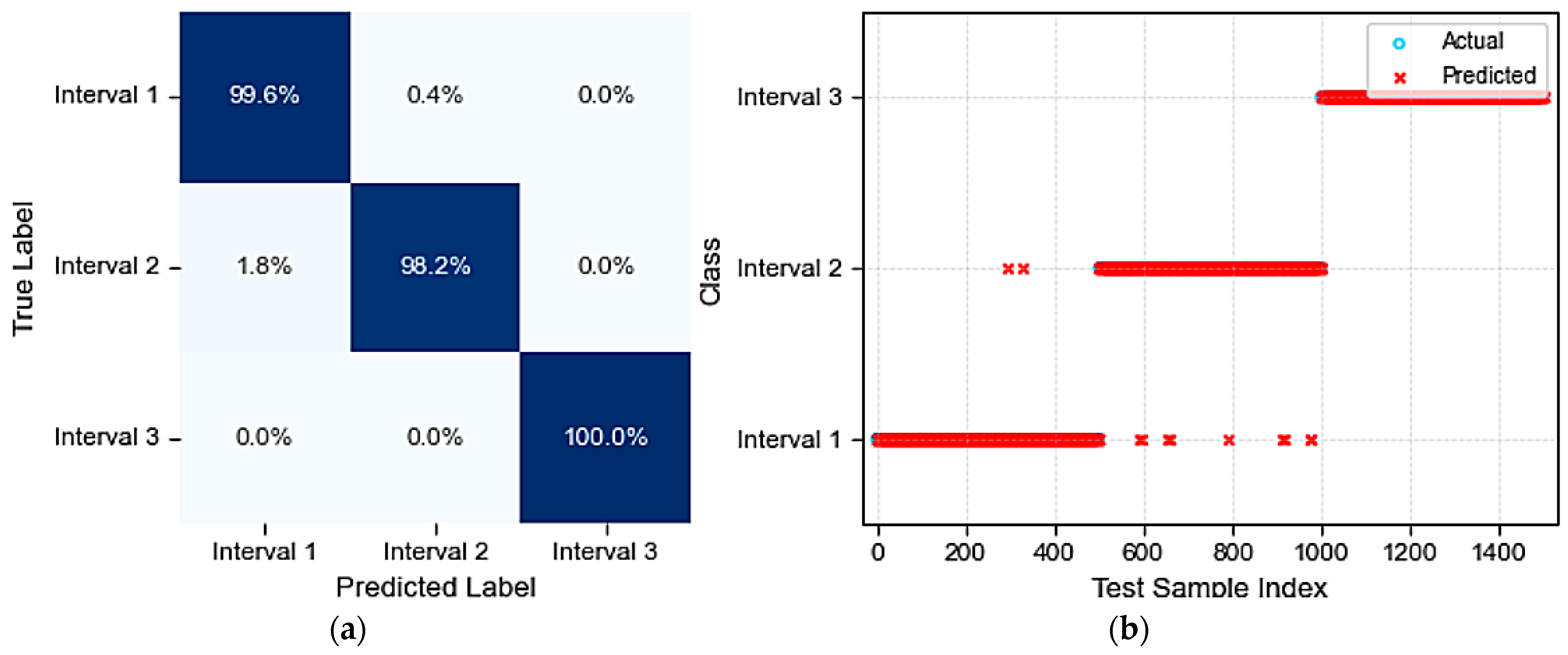
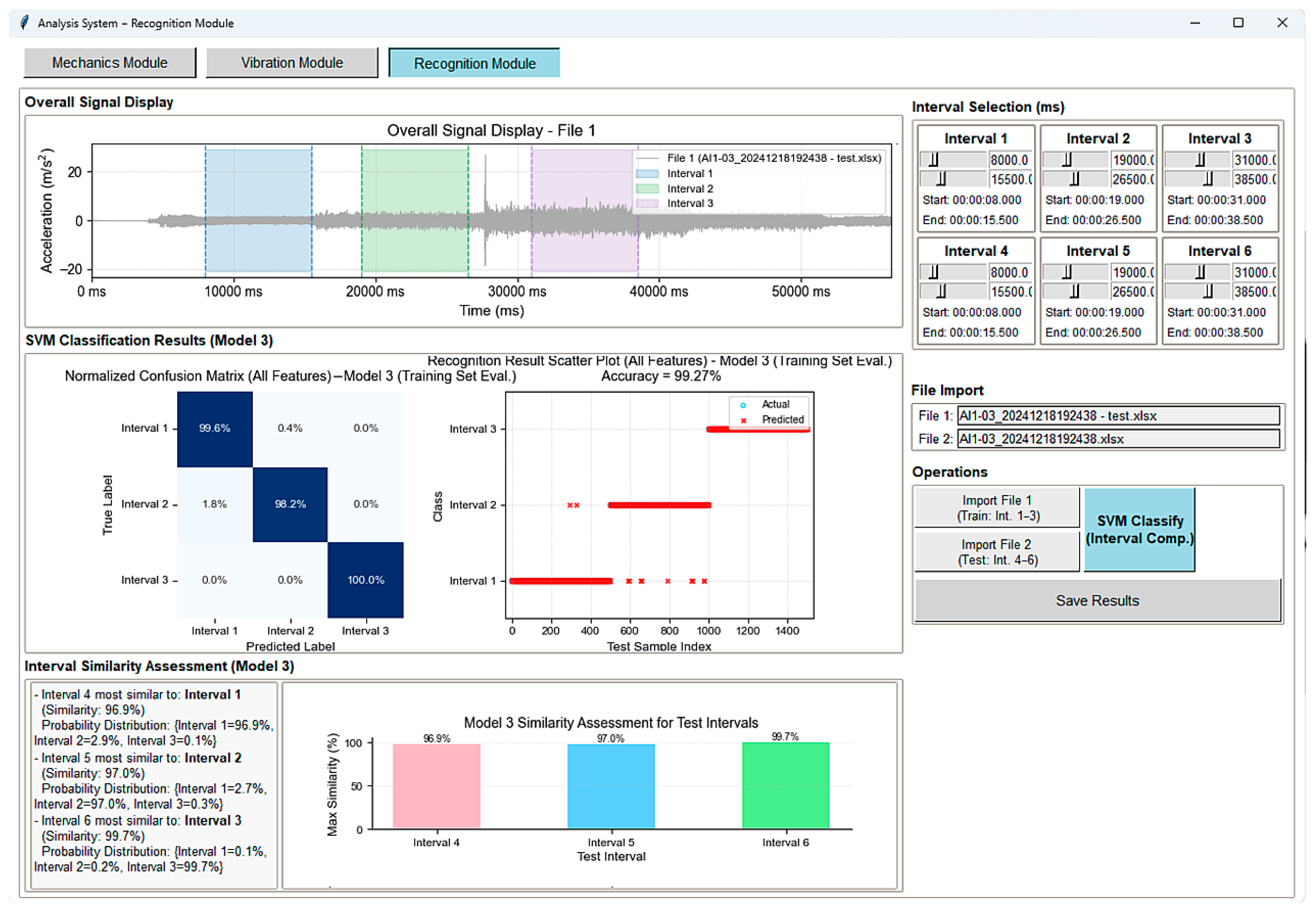
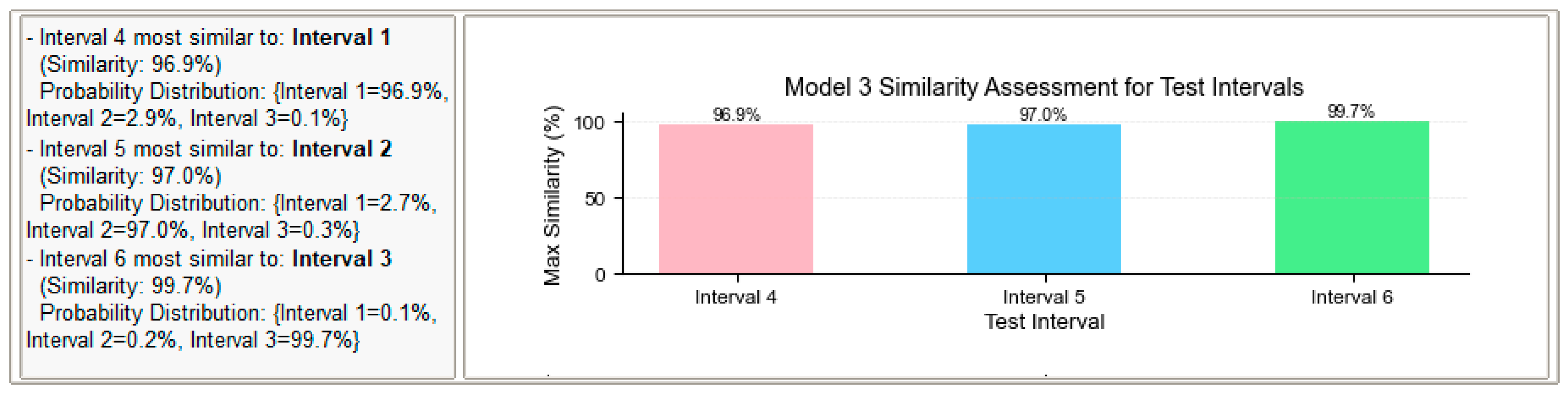
Based on a comparative analysis of several methodologies, including Support Vector Machines, Random Forest, Gradient Boosting Tree, XGBoost, LightGBM, and CatBoost, applied to the vigorously responding points identified through time-domain analysis, Support Vector Machines were determined to be the optimal classification method. Subsequently, employing a “one-vs.-one” (OvO) strategy, a state recognition model was established. The vibration signals from the aforementioned measurement point, acquired using the designed signal acquisition system, were then utilized to conduct a model recognition validation experiment. The established model demonstrated a classification accuracy of 96.9% for Work State 1, with misclassification rates of 2.9% as Work State 2 and 0.1% as Work State 3. For Work State 2, the model achieved a classification accuracy of 97.0%, with misclassification rates of 2.7% as Work State 1 and 0.3% as Work State 3. Work State 3 exhibited a classification accuracy of 99.7%, with misclassification rates of 0.1% as Work State 1 and 0.2% as Work State 2. Misclassification rates for all other intervals were consistently below 5%, indicating that precise judgment of the working state of the bolted structure is indeed achievable.

References

1. Ma, Z.; Wu, Z.P.; Li, Y.F.; Song, Z.Q.; Yu, J.; Li, Y.M.; Xu, L.Z. Study of the grain particle-conveying performance of a bionic non-smooth-structure screw conveyor. Biosyst. Eng. 2024, 238, 94–104. [Google Scholar] [CrossRef]
2. Li, Y.; Xu, L.Z.; Lv, L.Y.; Shi, Y.; Yu, X. Study on Modeling Method of a Multi-Parameter Control System for Threshing and Cleaning Devices in the Grain Combine Harvester. Agriculture 2022, 12, 1483. [Google Scholar] [CrossRef]
3. Qian, P.; Gu, J.; Tang, Z.; Lao, L.; Lu, T.; Gu, T.; Chen, S. Development and validation of the damped pendulum model for cantilever conveyor trough using Lagrangian method. Trans. Chin. Soc. Agric. Eng. 2023, 39, 44–52. [Google Scholar]
4. Li, Y.M.; Liu, Y.B.; Ji, K.Z.; Zhu, R.H. A Fault Diagnosis Method for a Differential Inverse Gearbox of a Crawler Combine Harvester Based on Order Analysis. Agriculture 2022, 12, 1300. [Google Scholar] [CrossRef]
5. Li, H.B.; Chen, L.W.; Zhang, Z.Y. A Study on the Utilization Rate and Influencing Factors of Small Agricultural Machinery: Evidence from 10 Hilly and Mountainous Provinces in China. Agriculture 2023, 13, 51. [Google Scholar] [CrossRef]
6. Gao, J.; Liu, Z.; Gu, W.; Zhang, F.; Zhu, L.; Xu, J. Modal Analysis and Optimization of Grain Combine Harvester Undercarriage Frame. Mach. Des. Res. 2023, 39, 199–205. [Google Scholar]
7. Chandio, F.A.; Li, Y.; Xu, L.; Ma, Z.; Xu, L.Z. Predicting 3D forces of disc tool and soil disturbance area using fuzzy logic model under sensor based soil-bin. Int. J. Agric. Biol. Eng. 2020, 13, 77–84. [Google Scholar] [CrossRef]
8. Pang, J.; Li, Y.M.; Ji, J.T.; Xu, L.Z. Vibration excitation identification and control of the cutter of a combine harvester using triaxial accelerometers and partial coherence sorting. Biosyst. Eng. 2019, 185, 25–34. [Google Scholar] [CrossRef]
9. Liang, Z.W.; Li, Y.M.; Xu, L.Z.; Zhao, Z. Sensor for monitoring rice grain sieve losses in combine harvesters. Biosyst. Eng. 2016, 147, 51–66. [Google Scholar] [CrossRef]
10. Chen, J.; Lian, Y.; Zou, R.; Zhang, S.; Ning, X.B.; Han, M.N. Real-time grain breakage sensing for rice combine harvesters using machine vision technology. Int. J. Agric. Biol. Eng. 2020, 13, 194–199. [Google Scholar] [CrossRef]
11. Zhang, Y.; Wu, C.; Jiang, Z.; Jiang, L.; Guan, Z.; Wang, G. Design and test of dust suppression system for rice-wheat combine harvesters. Trans. Chin. Soc. Agric. Eng. 2021, 37, 97–105. [Google Scholar]
12. He, C.; Jing, H.; Zhao, C.; Te, B.; Shi, L.; Tu, N. Design and Experiment of Cutting Device of Multi-degree-of-freedom Sandy Willow Harvester. Trans. Chin. Soc. Agric. Mach. 2024, 55, 320–328. [Google Scholar]
13. Luan, Y.; Yu, L.; Song, H.; Du, Y.; Gao, C.; Zhang, C. Design and experiment of a watercress harvesting device. J. Gansu Agric. Univ. 2023, 58, 246–254. [Google Scholar]
14. Feng, W.; Cui, J.; Li, P.; Cao, Z.; Li, Y.; Ding, X.; Zhan, X. Small Harvester Noise Reduction Design and Noise Source Analysis. Southwest China J. Agric. Sci. 2020, 33, 1081–1086. [Google Scholar]
15. Mao, J.F.; Li, D.H.; Yu, Z.W.; Cai, W.F.; Guo, W.; Zhang, G.W. A novel refined dynamic model of high-speed maglev train-bridge coupled system for random vibration and running safety assessment. J. Cent. South Univ. 2024, 31, 2532–2544. [Google Scholar] [CrossRef]
16. Chen, J.; Ning, X.; Li, Y.; Yang, G.; Wu, P.; Chen, S. A fuzzy control strategy for the forward speed of a combine harvester based on kdd. Appl. Eng. Agric. 2017, 33, 15–22. [Google Scholar] [CrossRef]
17. He, X.; Chen, X.; Qu, Z.; Lan, M.; Wang, W. Review on application research and development of intelligent technology in the process of wheat harvest. J. Henan Agric. Univ. 2022, 56, 341–354. [Google Scholar]
18. Lian, Y.; Chen, J.; Guan, Z.H.; Song, J. Development of a monitoring system for grain loss of paddy rice based on a decision tree algorithm. Int. J. Agric. Biol. Eng. 2021, 14, 224–229. [Google Scholar] [CrossRef]
19. Li, X.; Zhou, D. Product Design Requirement Information Visualization Approach for Intelligent Manufacturing Services. China Mech. Eng. 2020, 31, 871–881. [Google Scholar]
20. Liang, Z.W.; Li, Y.M.; De Baerdemaeker, J.; Xu, L.Z.; Saeys, W. Development and testing of a multi-duct cleaning device for tangential-longitudinal flow rice combine harvesters. Biosyst. Eng. 2019, 182, 95–106. [Google Scholar] [CrossRef]
21. Luo, Y.S.; Wei, L.L.; Xu, L.Z.; Zhang, Q.; Liu, J.Y.; Cai, Q.B.; Zhang, W.B. Stereo-vision-based multi-crop harvesting edge detection for precise automatic steering of combine harvester. Biosyst. Eng. 2022, 215, 115–128. [Google Scholar] [CrossRef]
22. Li, Z.; Zhang, F.; Teng, G.; Li, Z.; Wang, Z.; Ma, S. Deep reinforcement learning-based optimization strategy for the cooperative scheduling of harvesters. Trans. Chin. Soc. Agric. Eng. 2024, 40, 23–32. [Google Scholar]
23. Xi, C.; Yang, G.; Liu, L.; Liu, J.; Chen, X.; Ma, Z. Operation faults monitoring of combine harvester based on SDAE-BP. Trans. Chin. Soc. Agric. Eng. 2020, 36, 46–53. [Google Scholar]
24. Hu, X.; Hou, L.; Bu, X.; Zhou, Y. Vibration and noise analysis of fuel pump regulator under combined load. J. Aerosp. Power 2024, 39, 20220849. [Google Scholar]
25. Han, J.Y.; Yan, X.X.; Tang, H. Method of controlling tillage depth for agricultural tractors considering engine load characteristics. Biosyst. Eng. 2023, 227, 95–106. [Google Scholar] [CrossRef]
26. Han, J.Y.; Liu, C.H. Research on a Method to Measure and Calculate Tillage Resistance of Tractor Mounted Plough. AMA-Agric. Mech. Asia Afr. Lat. Am. 2018, 49, 67–73. [Google Scholar]
27. Jin, M.Z.; Zhao, Z.; Chen, S.R.; Chen, J.Y. Improved piezoelectric grain cleaning loss sensor based on adaptive neuro-fuzzy inference system. Precis. Agric. 2022, 23, 1174–1188. [Google Scholar] [CrossRef]
28. Wen, M.; Dang, Z.; Yu, Z.; Lu, Y.; Wei, G. Dynamic mode decomposition and its application in early bearing fault diagnosis. J. Vib. Shock. 2022, 41, 313–320. [Google Scholar]
29. Yang, S.; Zhai, C.Y.; Gao, Y.Y.; Dou, H.J.; Zhao, X.G.; He, Y.K.; Wang, X. Planting uniformity performance of motor-driven maize precision seeding systems. Int. J. Agric. Biol. Eng. 2022, 15, 101–108. [Google Scholar] [CrossRef]
30. Lu, C.; Li, X.; Yao, Y.; Tang, X.; Peng, Y.; Wang, S. Design and Implementation of Parallel Prediction Model for Aeroengine Multi-Sensor. J. Univ. Electron. Sci. Technol. China 2021, 50, 580–585. [Google Scholar]
31. Tan, P.; Qiu, L.; Ding, J.; Lin, J.; Li, Z.; Huang, W. Study on Monitoring Technology of Key Parameters of High-speed Railway Catenary Anchor Segment Terminal. Instrum. Tech. Sens. 2023, 2, 115–120. [Google Scholar]
32. Zhu, F.H.; Chen, J.; Guan, Z.H.; Zhu, Y.H.; Shi, H.; Cheng, K. Development of a combined harvester navigation control system based on visual simultaneous localization and mapping-inertial guidance fusion. J. Agric. Eng. 2024, 55. [Google Scholar] [CrossRef]
33. Wang, H.; Yang, Q.; Liu, Q.; Zhao, C.; Zhang, H. Productivity analysis of cable crane transportation based onvisual tracking and pattern recognition. J. Tsinghua Univ. Sci. Technol. 2024, 64, 1646–1657. [Google Scholar]
34. Pan, B.; Qian, Q.; Dai, S. A method for quick evaluating the capacity of lithium ion batteries under working conditions. Sci. Sin. Technol. 2024, 54, 835–847. [Google Scholar]
35. Wu, D.; He, Q. Study on Typical Fault Detection Method for Insufficient Turbine Rotor Fault Samples. Noise Vib. Control 2024, 44, 101–108. [Google Scholar]
36. Zhao, P.; Wang, X.; Fu, M. Few-shot switch machine fault diagnosis based on Bayesian meta-learning. J. Railw. Sci. Eng. 2023, 20, 4008–4020. [Google Scholar]
37. Liu, Y.; Zhou, E.; Zhang, W.; Wang, X.; Lv, F. Classification of Robot Execution Failures Using a Spike-CNN Model Underlying STDP Learning by Reward and Punishment Mechanisms. J. Chin. Comput. Syst. 2022, 43, 1285–1292. [Google Scholar]
38. Chen, Y.X.; Chen, L.; Wang, R.C.; Xu, X.; Shen, Y.J.; Liu, Y.L. Modeling and test on height adjustment system of electrically-controlled air suspension for agricultural vehicles. Int. J. Agric. Biol. Eng. 2016, 9, 40–47. [Google Scholar] [CrossRef]
39. Zang, C.; Zeng, J.; Li, P.; Liu, H.; Zhang, Z.; Sun, L.; Liu, Y. Intelligent Diagnosis Model of Mechanical Fault for Power Transformer Based on SVM Algorithm. High Volt. Appar. 2023, 59, 216. [Google Scholar]
40. Ju, D.; Wu, Y.; Ma, B.; Li, X. Digital Modeling and Dynamic Simulation Analysis of Gear Transmission System in Bolt Fault State. J. Eng. Therm. Energy Power 2024, 39, 168–174. [Google Scholar]
41. Huang, X.Y.; Yu, S.S.; Xu, H.X.; Aheto, J.H.; Bonah, E.; Ma, M.; Wu, M.; Zhang, X.R. Rapid and nondestructive detection of freshness quality of postharvest spinaches based on machine vision and electronic nose. J. Food Saf. 2019, 39, e12708. [Google Scholar] [CrossRef]
42. Wan, Y.; Xue, J.; Zhang, D.; Han, X.; Lyu, J.; Miao, W. Research on bolts fault diagnosis of diaphragm compressor cylinder head in nuclear power plant based on KPCA. Fluid Mach. 2024, 52, 87–96. [Google Scholar]
43. Qian, J.; Chen, G.; Cun, W.; Zhao, X.; Zhang, X.; Zhao, Z. High-Fidelity Finite Element Simulation and Experimental Verification of Bolt Preload Force Under Tightening Torque. J. Mech. Strength 2024, 46, 809–815. [Google Scholar]
44. Zhao, X.; Zhang, J.; Pan, Y.; Fan, F.; Zhang, Y. Research on Delayed Fracture of High-Strength Bolts in Steel Bridge. Bridge Constr. 2024, 54, 47–54. [Google Scholar]
45. Chen, P.; Shang, Q.; Yu, X.; Yin, A. Ultrasonic multi-feature fusion bolt stress measurement method based on ELM. Chin. J. Sci. Instrum. 2024, 45, 46–56. [Google Scholar]
46. Li, X.; Lai, B.; Zhang, A.; Li, G. Detection of bolt fastening state of locomotive bogie based on image recognition. J. Electron. Meas. Instrum. 2023, 37, 143–155. [Google Scholar]
47. Guo, Z.; Zhao, W.; Chen, H.; Lyu, S. Research on a Detection Method for Loosening of High-Strength Bolts Based on Image Recognition Techniques. Ind. Constr. 2022, 52, 175. [Google Scholar]
48. Zhang, Z.; Zhou, L.; Liu, S. A Study on Key Factors Affecting Bolt Looseness of Aeolian Vibration Dampers under Lateral Vibration Conditions. Power Syst. Clean Energy 2024, 40, 11–17. [Google Scholar]
49. Dong, H.; Yao, J.; He, C.; Li, J. Visual detection algorithm of loose fasteners under the subway. J. Railw. Sci. Eng. 2024, 21, 3775–3786. [Google Scholar]
50. Li, S.; Xue, Y.; Chi, S.; Fan, X.; Zhang, Y.; Yang, W. Intelligent lost and loose detection of track fastener components based on 3D camera. J. Railw. Sci. Eng. 2024, 21, 386–395. [Google Scholar]
Figure 1. DH5902N Dynamic acquisition instrument and DHDAS dynamic signal acquisition and analysis system.
Agriculture 15 00970 g001
Figure 2. Bolted Structure Vibration Response Test Procedure.
Agriculture 15 00970 g002
Figure 3. Measurement points and coordinate system for measurement directions in the bolted structure vibration test.
Agriculture 15 00970 g003
Figure 4. Configuration of DHDAS Dynamic Acquisition System Channels and Sensor Parameters.
Agriculture 15 00970 g004
Figure 5. Configuration of DHDAS Dynamic Acquisition System Channels and Sensor Parameters. (a) Channel Parameter Settings; (b) Relationship between Electrical Quantity and Physical Quantity.
Agriculture 15 00970 g005
Figure 6. Schematic Diagram of the SVM Classification and Identification Principle.
Agriculture 15 00970 g006
Figure 7. The Random Forest Classification Principle.
Agriculture 15 00970 g007
Figure 8. The Bayesian optimization hyperparameter of the SVM identification method.
Agriculture 15 00970 g008
Figure 9. Power supply circuit for the vibration signal acquisition system. (a) 220 V step-down to 12 V and 5 V circuit; (b) 5 V to 1.2 V LED circuit.
Agriculture 15 00970 g009
Figure 10. Sensor Multi-Channel Acquisition Module. (a) ADS1299 ADC Core and Digital Interface Module; (b) Analog Signal Input Interface Module; (c) ADS1299 ADC Connection Circuit.
Agriculture 15 00970 g010
Figure 11. The 3.3 V to 5 V Level Shifting Module.
Agriculture 15 00970 g011
Figure 12. Wireless Main Control Debugging and Interface Circuits. (a) Wireless Main Control Debugging Circuit; (b) Interface Circuit.
Agriculture 15 00970 g012
Figure 13. Conveyor Trough Vibration Signal Acquisition System.
Agriculture 15 00970 g013
Figure 14. Host Computer Software for Signal Acquisition System.
Agriculture 15 00970 g014
Figure 15. Time domain characteristics of the vibration signal in the X direction of each measuring point of the conveying tank.
Agriculture 15 00970 g015
Figure 16. Time domain characteristics of the vibration signal in the Y direction of each measuring point of the conveying tank.
Agriculture 15 00970 g016
Figure 17. Time domain characteristics of the vibration signal in the Z direction of each measuring point of the conveying tank.
Agriculture 15 00970 g017
Figure 18. Prediction Results for Interval 1 and Interval 2. (a) Signal Waveforms for Interval 1 and Interval 2; (b) Confusion Matrix for Interval 1 and Interval 2; (c) Recognition Scatter Plot for Interval 1 and Interval 2.
Agriculture 15 00970 g018
Figure 19. Prediction Results for Interval 2 and Interval 3. (a) Signal Waveforms for Interval 2 and Interval 3; (b) Confusion Matrix for Interval 2 and Interval 3; (c) Recognition Scatter Plot for Interval 2 and Interval 3.
Agriculture 15 00970 g019
Figure 20. Prediction Results for Three Intervals. (a) Confusion Matrix for Three Intervals; (b) Scatter Plot of Recognition Results for Three Intervals.
Agriculture 15 00970 g020
Figure 21. Performance Test Experiment of Signal Acquisition System.
Agriculture 15 00970 g021
Figure 22. Work State Recognition Program for Bolted Structure.
Agriculture 15 00970 g022
Figure 23. Work State Recognition Results for Bolted Joint Location.
Agriculture 15 00970 g023